Embed Size (px)
Citation preview
On the origin of Phase Transitions in the absence of
Symmetry-Breaking
Giulio Pettini,1, ∗ Matteo Gori,2, † Roberto
Franzosi,3, ‡ Cecilia Clementi,4, § and Marco Pettini2, ¶
1Dipartimento di Fisica Universita di Firenze, and I.N.F.N.,
Sezione di Firenze, via G. Sansone 1, I-50019 Sesto Fiorentino, Italy
2Centre de Physique Theorique, Aix-Marseille University,
Campus de Luminy, Case 907, 13288 Marseille Cedex 09, France
3QSTAR and INO-CNR, largo Enrico Fermi 2, I-50125 Firenze, Italy
4Department of Chemistry, Rice University,
6100 Main street, Houston, TX 77005-1892, USA
(Dated: September 7, 2018)
Abstract
In this paper we investigate the Hamiltonian dynamics of a lattice gauge model in three spatial
dimensions. Our model Hamiltonian is defined on the basis of a continuum version of a duality
transformation of a three dimensional Ising model. The system so obtained undergoes a thermo-
dynamic phase transition in the absence of a global symmetry-breaking and thus in the absence of
an order parameter. It is found that the first order phase transition undergone by this model fits
into a microcanonical version of an Ehrenfest-like classification of phase transitions applied to the
configurational entropy. It is discussed why the seemingly divergent behaviour of the third deriva-
tive of configurational entropy is the effect of a deeper geometrical transition of the equipotential
submanifolds of configuration space, which, in its turn, is likely to be the ”shadow” of an even
deeper transition of topological kind.
Keywords: microcanonical phase transitions; topology and phase transitions; Hamiltonian dy-
namics and phase transitions
PACS numbers: 05.45.+b; 02.40.-k; 05.20.-y
∗ [email protected]† [email protected]‡ [email protected]§ [email protected]¶ [email protected]
1
I. INTRODUCTION
One of the main topics in Statistical Mechanics concerns phase transitions phenomena.
From the theoretical viewpoint, understanding their origin, and the way of classifying them,
is of central interest.
Usually, phase transitions are associated with a spontaneous symmetry-breaking phe-
nomenon: at low temperatures the accessible states of a system can lack some of the global
symmetries of the Hamiltonian, so that the corresponding phase is the less symmetric one,
whereas at higher temperatures the thermal fluctuations allow the access to a wider range
of energy states having all the symmetries of the Hamiltonian. In the symmetry-breaking
phenomena, the extra variable which characterizes the physical states of a system is the or-
der parameter. The order parameter vanishes in the symmetric phase and is different from
zero in the broken-symmetry phase. This is the essence of Landau’s theory. If G0 is the
global symmetry group of the Hamiltonian, the order of a phase transition is determined
by the index of the subgroup G ⊂ G0 of the broken symmetry phase. The corresponding
mechanism in quantum field theory is described by the Nambu-Goldstone’s Theorem.
However, this is not an all-encompassing theory. In fact, many systems do not fit in this
scheme and undergo a phase transition in the absence of a symmetry-breaking. This is the
case of liquid-gas transitions, Kosterlitz-Thouless transitions, coulombian/confined regime
transition for gauge theories on lattice, transitions in glasses and supercooled liquids, in
general, transitions in amorphous and disordered systems, folding transitions in homopoly-
mers and proteins, to quote remarkable examples. All these physical systems lack an order
parameter.
Moreover, classical theories, as those of Yang-Lee [2] and of Dobrushin-Lanford-Ruelle [3],
require the N →∞ limit (thermodynamic limit) to mathematically describe a phase transi-
tion, but the study of transitional phenomena in finite N systems is particularly relevant in
many other contemporary problems [4], for instance related with polymers thermodynamics
and biophysics [5], with Bose-Einstein condensation, Dicke’s superradiance in microlasers,
nuclear physics [6], superconductive transitions in small metallic objects. The topological
theory of phase transitions provides a natural framework to get rid of the thermodynamic
limit dogma because clear topological signatures of phase transitions are found already at
finite and small N [7, 13].
2
Therefore, looking for generalisations of the existing theories is a well motivated and
timely purpose. The present paper aims at giving a contribution in this direction along a
line of thought initiated several years ago with the investigation of the Hamiltonian dynam-
ical counterpart of phase transitions [7–9] which eventually led to formulate a topological
hypothesis. In fact, Hamiltonian flows (H-flows) can be seen as geodesic flows on suitable
Riemannian manifolds [7, 10], and then the question naturally arises of whether and how
these manifolds “encode” the fact that their geodesic flows/H-flows are associated or not
with a thermodynamic phase transition (TDPT). It is by following this conceptual pathway
that one is eventually led to hypothesize that suitable topological changes of certain sub-
manifolds of phase space are the deep origin of TDPT. This hypothesis was corroborated
by several studies on specific exactly solvable models [11–15] and by two theorems. These
theorems, even if still somewhat controversial [16], state that the unbounded growth with
N of relevant thermodynamic quantities, eventually leading to singularities in the N →∞
limit - the hallmark of an equilibrium phase transition - is necessarily due to appropriate
topological transitions in configuration space [7, 17–19].
Hence, and more precisely, the present paper aims at investigating whether also TDPT
occurring in the absence of symmetry-breaking, and thus in the absence of an order pa-
rameter, can be ascribed to some major geometrical change of the previously mentioned
manifolds, possibly rooted in a deeper topological change of these same manifolds.
To this purpose, inspired by the dual Ising model, we define a continuous variables Hamil-
tonian in three spatial dimensions (3D) having the same local (gauge) symmetry of the dual
Ising model (reported in Section II) and then proceed to its numerical investigation. The
results are reported and discussed in Section III. Through a standard analysis of thermody-
namic observables, it is found that this model undergoes a first order phase transition. It is
also found that the larger the number of degrees of freedom the sharper the jump of the sec-
ond derivative of configurational entropy, what naturally fits into a proposed microcanonical
version of an Ehrenfest-like classification of phase transitions.
A crucial finding of the present work consists of the observation that this jump of the
second derivative of configurational entropy coincides with a jump of the second derivative
of a geometric quantity measuring the total dispersion of the principal curvatures of certain
submanifolds (the potential level sets) of configuration space. This is a highly non trivial
fact because the peculiar energy variation of the geometry of these submanifolds, entailing
3
the jump of the second derivative of the total dispersion of their principal curvatures, is
a primitive, a fundamental phenomenon: it is the cause and not the effect of the energy
dependence of the entropy and its derivatives, that is, the phase transition is a consequence
of a deeper phenomenon. In its turn, the peculiar energy-pattern of this geometric quantity
appears to be rooted in the variations of topology of the potential level sets, thus the present
results provide a further argument in favour of the topological theory of phase transitions,
also in the absence of symmetry-breaking.
II. THE MODEL
Starting from the Ising Hamiltonian
Vising
(σii∈Λ
)= −J
∑〈ij〉∈Λ
σiσj (1)
with nearest-neighbor interactions (〈ij〉) on a 3D-lattice Λ, where the σi are discrete di-
chotomic variables (σi = ±1) defined on the lattice sites and J is real positive (ferromagnetic
coupling), one defines the potential energy of the dual model [20]
Vdual (U) = −J∑
UijUjkUklUli (2)
where the discrete variables Umm′ are defined on the links joining the sites m and m′, and
Umm′ = ±1. The summation is carried over all the minimal plaquettes (denoted by ) into
which the lattice can be decomposed. The dual model in (2) has the local (gauge) symmetry
Uij → εiεjUij (3)
with εi, εj = ±1, and i, j ∈ Λ. Such a gauge transformation leaves the model (2) unaltered,
and after the Elitzur theorem [21] 〈Uij〉 does not qualify as a good order parameter to detect
the occurrence of a phase transition because 〈Uij〉 = 0 always. In other words, no bifurcation
of 〈Uij〉 can be observed at any phase transition point inherited by the model (2) from the
Ising model (1).
In order to define a Hamiltonian flow with the same property of local symmetry – hin-
dering the existence of a standard order parameter – we borrow the analytic form of (2) and
replace the discrete dichotomic variables Uij with continuous ones Uij ∈ R. We remark that
4
we donot want to investigate the dual-Ising model, rather we just heuristically refer to it in
order to define a gauge model with the desired properties.
Moreover, we add to the continuous version of (2) a stabilizing term which is invariant
under the same local gauge transformation (3); this reads
Vquartic(U) = α∑〈ij〉
(U2ij − 1
)4, (4)
where 〈ij〉 stands for nearest-neighbor interactions for link variables and α is a real positive
coupling constant.
On a 3D-lattice Λ, and with I = (1, 0, 0), (0, 1, 0), (0, 0, 1), we thus define the following
model Hamiltonian
H(π, U) =K(π) + Vising(U) + Vquartic(U) =
=∑i∈Λ
∑µ∈I
1
2π2iµ − J
∑∈Λ
UijUjkUklUli + α∑i∈Λ
∑µ∈I
(U2iµ − 1
)4 (5)
whose flow is investigated through the numerical integration of the corresponding Hamilton
equations of motion.
A more explicit form of (5) is given by
H(π, U) =n∑
i,j,k=1
3∑ν=1
1
2π2ijkν − J
n∑i,j,k=1
[Uijk1Ui+1jk2Uij+1k1Uijk2 (6)
+ Uijk2Uij+1k3Uijk+12Uijk3 + Uijk3Uijk+11Ui+1jk3Uijk1] + αn∑
i,j,k=1
3∑ν=1
(U2ijkν − 1
)4,
where the summation is carried over trihedrals made of three orthogonal plaquettes. Here
Uijk1 is the link variable joining the sites (i, j, k) and (i + 1, j, k), Uijk2 is the link variable
joining the sites (i, j, k) and (i, j + 1, k), Uijk3 is the link variable joining the sites (i, j, k)
and (i, j, k+1). Similarly, for example, Ui+1jk2 joins the sites (i+1, j, k) and (i+1, j+1, k),
Uij+1k1 joins (i+ 1, j+ 1, k) and (i, j+ 1, k), and so on. That is to say that the fourth index
labels the direction, i.e which index is varied by one unit.
The Hamilton equations of motion are given by
Uijkν = πijkν ,
πijkν = − ∂H∂Uijkν
, i, j, k = 1, . . . , n; ν = 1, 2, 3, (7)
periodic boundary conditions are always assumed.
5
The numerical integration of these equations is correctly performed only by means of
symplectic integration schemes. These algorithms satisfy energy conservation (with zero
mean fluctuations around a reference value of the energy) for arbitrarily long times as well
as the conservation of all the Poincare invariants, which include the phase space volume, so
that also Liouville’s theorem is satisfied by a symplectic integration. We adopted a third-
order bilateral symplectic algorithm as described in [22]. We used J = 1 and α = 1, the
integration time step ∆t varied from 0.005 at low energy to 0.001 at high energy so as to
keep the relative energy fluctuations ∆E/E close to 10−6.
III. DEFINITION OF THE OBSERVABLES AND NUMERICAL INVESTIGA-
TION
Given any observable A = A(π, U), one computes its time average as
〈A〉t =1
t
∫ t
0
dτ A[π(τ), U(τ)] (8)
along the numerically computed phase space trajectories. For sufficiently long integration
times, and for generic nonlinear (chaotic) systems, these time averages are used as estimates
of microcanonical ensemble averages in all the expressions given below.
A. Thermodynamic observables
The basic macroscopic thermodynamic observable is temperature. The microcanonical
definition of temperature depends on entropy — the basic thermodynamic potential in the
microcanonical ensemble — according to the relation
1
T=
(∂S
∂E
)V, (9)
where V is the volume, E is the energy and the entropy S is given by
S(N,E,V) = kB log
∫dπ1 · · · dπNdU1 · · · dUN δ[E −H(π, U)] (10)
where N is the total number of degrees of freedom, N = 3n3 in the present context, and Uk
stands for any suitable labelling of them. By means of a Laplace transform technique [23],
from Eqs. (9) and (10) one gets (setting kB = 1)
T = 2[(N − 2)〈K−1〉
]−1. (11)
6
where 〈K−1〉 is the microcanonical ensemble average of the inverse of the kinetic energy
K = E − V (U), where V (U) is the potential part of the Hamiltonian (7).
In numerical simulations
〈K−1〉 =1
t
∫ t
0
dτ
[n∑
i,j,k=1
3∑ν=1
1
2π2ijkν(τ)
]−1
. (12)
For t sufficiently large 〈K−1〉 attains a stable value (in general this is a rapidly converging
quantity entailing a rapid convergence of T ).
Since the invariant measure for nonintegrable Hamiltonian dynamics is the microcanonical
measure in phase space, the occurrence of equilibrium phase transitions can be investigated
in the microcanonical statistical ensemble through Hamiltonian dynamics [7, 24]. Standard
numerical signatures of phase transitions (also found with canonical Monte Carlo random
walks in phase space) are: the bifurcation of the order parameter at the transition point
(somewhat smoothed at finite number of degrees of freedom), and sharp peaks – of increasing
height with an increasing number of degrees of freedom – of the specific heat at the transition
point. As already remarked above, our model (7), because of the local (gauge) symmetry,
lacks a standard definition of an order parameter as is usually given in the case of symmetry-
breaking phase transitions. And in fact, in every numerical simulation of the dynamics we
have computed the time average 〈〈Uij〉〉t always finding 〈〈Uij〉〉t ' 0 independently of the
lattice size and of the energy value (the double average means averaging over the entire
lattice first, and then averaging over time).
Thus, the presence of a phase transition is detected through the shape of the so-called
caloric curve, that is, T = T (E). For the model in (7) this has been computed by means of
Eq. (11). Then the microcanonical constant-volume specific heat follows according to the
relation 1/CV = ∂T (E)/∂E. The numerical computation of specific heat can be indepen-
dently performed, with respect to the caloric curve, as follows. Starting with the definition
of the entropy, given in (10), an analytic formula can be worked out [23], which is exact at
any value of N . This formula reads
cV(E) =CVN
=N(N − 2)
4
[(N − 2)− (N − 4)
〈K−2〉〈K−1〉2
]−1
, (13)
and this is the natural expression to work out the microcanonical specific heat by means of
Hamiltonian dynamical simulations.
7
In order to get the above defined specific heat, time averages of the kind
〈Kα〉t =1
t
∫ t
0
dτ
[n∑
i,j,k=1
3∑ν=1
1
2π2ijkν(τ)
]αare computed with α = −1,−2. Then, for sufficiently large t, the microcanonical averages
〈Kα〉 can be replaced by 〈Kα〉t.
−3 −2 −1 0 1 2 30
1
2
3
4
5
E/N
T
1.2
1.3
1.4
1.5
1.6
1.7
1.8
1.9
2
2.1
-1.5 -1 -0.5 0 0.5 1
T
E/N
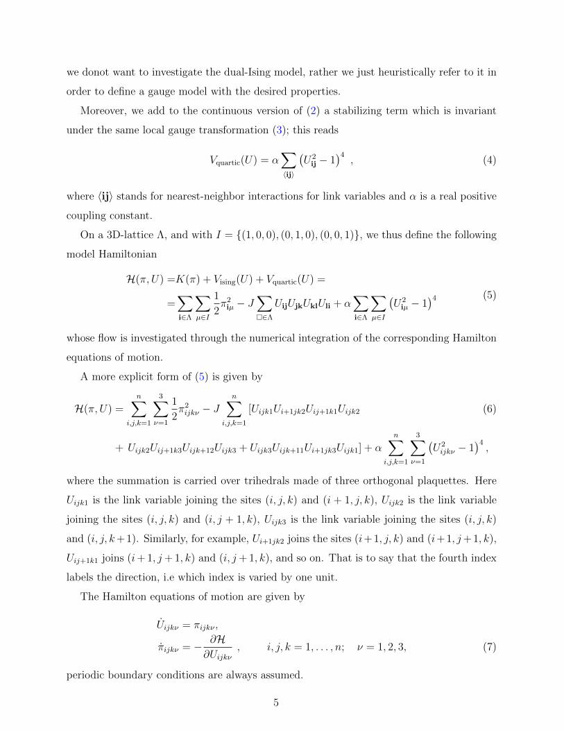
Figure 1. Caloric curve. The temperature, computed according to Eq.(11) is reported versus E/N .
Lattice dimensions: n3 = 6× 6× 6 (rhombs), n3 = 8× 8× 8 (squares), n3 = 10× 10× 10 (circles),
n3 = 14×14×14 (full circles). The dashed lines identify the point of flat tangency at lower energy.
The right panel is a zoom of the central part of the left panel.
In Figure 1 the caloric curve is reported for different sizes of the lattice. A kink, typical of
first order phase transitions, can be seen. This entails the presence of negative values of the
specific heat, and, consequently, ensemble nonequivalence for the model under consideration.
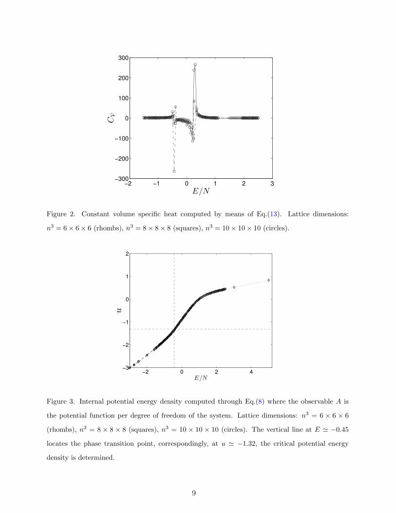
And, in fact, in Figure 2, where we report the outcomes of the computations of the specific
heat according to Eq.(13), we can observe an energy interval where the specific heat CV is
negative, and very high peaks are also found. Nevertheless, at this stage these peaks can
be attributed only to the existence of two points of flat tangency to the caloric curve and
cannot yet be attributed to an analyticity loss of the entropy (see Section III C).
In Figure 3 the average potential energy per lattice site u = 〈V 〉/N is displayed as a
function of the total energy density. Also in this case we observe a regular function which is
stable with the number of degrees of freedom. The dashed lines identify the phase transition
point which corresponds to Ec/N ' −0.45 and uc ' −1.32.
8
−2 −1 0 1 2 3−300
−200
−100
0
100
200
300
E/N
CV
Figure 2. Constant volume specific heat computed by means of Eq.(13). Lattice dimensions:
n3 = 6× 6× 6 (rhombs), n3 = 8× 8× 8 (squares), n3 = 10× 10× 10 (circles).
−2 0 2 4−3
−2
−1
0
1
2
E/N
u
Figure 3. Internal potential energy density computed through Eq.(8) where the observable A is
the potential function per degree of freedom of the system. Lattice dimensions: n3 = 6 × 6 × 6
(rhombs), n3 = 8 × 8 × 8 (squares), n3 = 10 × 10 × 10 (circles). The vertical line at E ' −0.45
locates the phase transition point, correspondingly, at u ' −1.32, the critical potential energy
density is determined.
9
The results so far reported provide us with a standard numerical evidence of the exis-
tence of a first order phase transition undergone by the model investigated. Besides standard
thermodynamic observables, the study of phase transitions through Hamiltonian dynamics
makes available a new observable, the largest Lyapunov exponent λ, which is of purely dy-
namical kind, and which has usually displayed peculiar patterns in presence of a symmetry-
breaking phase transition [7, 9, 25, 27–30]. Therefore in the following Section an attempt is
made to characterise the phase transition undergone by our model also through the energy
dependence of λ.
B. A Dynamic observable: the largest Lyapunov exponent
The largest Lyapounov exponent λ is the standard and most relevant indicator of the
dynamical stability/instability (chaos) of phase space trajectories. Let us quickly recall that
the numerical computation of λ proceeds by integrating the tangent dynamics equations,
which, for Hamiltonian flows, read
ξi = ζi ,
ζi = −N∑j=1
(∂2V
∂q1∂qj
)q(t)
ξj , i = 1, . . . , N (14)
together with the equations of motion of the Hamiltonian system under investigation. Then
the largest Lyapunov exponent λ is defined by
λ = limt→∞
1
tlog
[ξ21(t) + · · ·+ ξ2
N(t) + ζ21 (t) + · · ·+ ζ2
N(t)]1/2
[ξ21(0) + · · ·+ ξ2
N(0) + ζ21 (0) + · · ·+ ζ2
N(0)]1/2
, (15)
In a numerical computation the discretized version of (15) is used, with ξ = (ξ1, . . . , ξ2N)
and ξi+N = ξi
λ = limm→∞
1
m
m∑i=1
1
∆tlog‖ξ[(i+ 1)∆t]‖‖ξ(i∆t)‖
, (16)
where, after a given number of time steps ∆t, for practical numerical reasons it is convenient
to renormalize the value of ‖ξ‖ to a fixed one. The numerical estimate of λ is obtained by
retaining the time asymptotic value of λ(m∆t). This is obtained by checking the relaxation
pattern of log λ(m∆t) versus log(m∆t).
Note that λ can be expressed as the time average of a suitable observable defined as
10
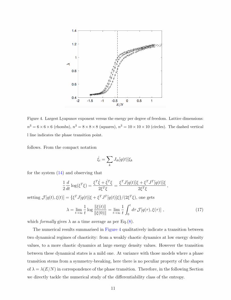
Figure 4. Largest Lyapunov exponent versus the energy per degree of freedom. Lattice dimensions:
n3 = 6× 6× 6 (rhombs), n3 = 8× 8× 8 (squares), n3 = 10× 10× 10 (circles). The dashed vertical
l line indicates the phase transition point.
follows. From the compact notation
ξi =∑k
Jik[q(t)]ξk
for the system (14) and observing that
1
2
d
dtlog(ξT ξ) =
ξT ξ + ξT ξ
2ξT ξ=ξTJ [q(t)]ξ + ξTJT [q(t)]ξ
2ξT ξ,
setting J [q(t), ξ(t)] = ξTJ [q(t)]ξ + ξTJT [q(t)]ξ/(2ξT ξ), one gets
λ = limt→∞
1
tlog‖ξ(t)‖‖ξ(0)‖
= limt→∞
1
t
∫ t
0
dτ J [q(τ), ξ(τ)] , (17)
which formally gives λ as a time average as per Eq.(8).
The numerical results summarised in Figure 4 qualitatively indicate a transition between
two dynamical regimes of chaoticity: from a weakly chaotic dynamics at low energy density
values, to a more chaotic dynamics at large energy density values. However the transition
between these dynamical states is a mild one. At variance with those models where a phase
transition stems from a symmetry-breaking, here there is no peculiar property of the shapes
of λ = λ(E/N) in correspondence of the phase transition. Therefore, in the following Section
we directly tackle the numerical study of the differentiability class of the entropy.
11
C. Microcanonical definition of phase transitions
In recent times, the problem of tackling equilibrium phase transitions in the microcanon-
ical ensemble has attracted increasing interest [4, 31–35], being of fundamental importance
in presence of ensemble inequivalence, or in the case of a dynamical approach based on
Hamiltonian dynamics, to quote just a few examples. At the end of the present Section, we
will take advantage especially of a recent and very interesting proposal in Ref.[35] which,
on the one side allows to give a coherent interpretation of our results, and on the other side
can be given some complementary support by what will be discussed in the following. Let
us begin, however, with a somewhat different/complementary viewpoint. As is well known,
according to the Ehrenfest classification, the order of a phase transition is given by the order
of the discontinuous derivative with respect to temperature T of the Helmholtz free energy
F (T ). However, a difficulty arises in presence of divergent specific heat CV associated with a
second order phase transition because this implies a divergence of (∂2F/∂T 2), and, in turn,
a discontinuity of (∂F/∂T ) so that the distinction between first and second order transi-
tions is lost. By resorting to the concept of symmetry-breaking, Landau theory circumvents
this difficulty by classifying the order of a phase transition according to the index of the
symmetry group of the broken-symmetry phase which is a subgroup of the group of the
more-symmetric phase. As in the present work we are tackling a system undergoing a phase
transition in the absence of symmetry-breaking, we have to get back to the origins as follows.
According to the Ehrenfest theory, a phase transition is associated with a loss of analyticity
of a thermodynamic potential (Helmholtz free energy, or, equivalently Gibbs free energy),
and the order of the transition depends on the differentiability class of this thermodynamic
potential. Later, on a mathematically rigorous ground, the identification of a phase transi-
tion with an analyticity loss of a thermodynamic potential (in the gran-canonical ensemble)
was confirmed by the Yang-Lee theorem. Now, let us consider the statistical ensemble which
is the natural counterpart of microscopic Hamiltonian dynamics, that is, microcanonical en-
semble. As already recalled in Section III.A, here the relevant thermodynamic potential is
entropy, and considering the specific heat
C−1V =
∂T (E)
∂Ewhich, after Eq.(9), reads CV = −
(∂S
∂E
)2(∂2S
∂E2
)−1
, (18)
from the last expression we see that CV can diverge only as a consequence of the vanishing
12
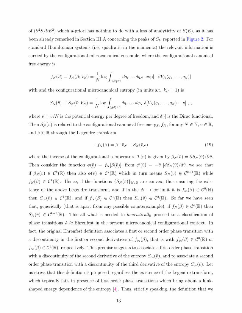
of (∂2S/∂E2) which a-priori has nothing to do with a loss of analyticity of S(E), as it has
been already remarked in Section III.A concerning the peaks of CV reported in Figure 2. For
standard Hamiltonian systems (i.e. quadratic in the momenta) the relevant information is
carried by the configurational microcanonical ensemble, where the configurational canonical
free energy is
fN(β) ≡ fN(β;VN) =1
Nlog
∫(Λd)×n
dq1 . . . dqN exp[−βVN(q1, . . . , qN)]
with and the configurational microcanonical entropy (in units s.t. kB = 1) is
SN(v) ≡ SN(v;VN) =1
Nlog
∫(Λd)×n
dq1 · · · dqN δ[VN(q1, . . . , qN)− v] , ,
where v = v/N is the potential energy per degree of freedom, and δ[·] is the Dirac functional.
Then SN(v) is related to the configurational canonical free energy, fN , for any N ∈ N, v ∈ R,
and β ∈ R through the Legendre transform
−fN(β) = β · vN − SN(vN) (19)
where the inverse of the configurational temperature T (v) is given by βN(v) = ∂SN(v)/∂v.
Then consider the function φ(v) = fN [β(v)], from φ′(v) = −v [dβN(v)/dv] we see that
if βN(v) ∈ Ck(R) then also φ(v) ∈ Ck(R) which in turn means SN(v) ∈ Ck+1(R) while
fN(β) ∈ Ck(R). Hence, if the functions SN(v)N∈N are convex, thus ensuring the exis-
tence of the above Legendre transform, and if in the N → ∞ limit it is f∞(β) ∈ C0(R)
then S∞(v) ∈ C1(R), and if f∞(β) ∈ C1(R) then S∞(v) ∈ C2(R). So far we have seen
that, generically (that is apart from any possible counterexample), if fN(β) ∈ Ck(R) then
SN(v) ∈ Ck+1(R). This all what is needed to heuristically proceed to a classification of
phase transitions a la Ehrenfest in the present microcanonical configurational context. In
fact, the original Ehrenfest definition associates a first or second order phase transition with
a discontinuity in the first or second derivatives of f∞(β), that is with f∞(β) ∈ C0(R) or
f∞(β) ∈ C1(R), respectively. This premise suggests to associate a first order phase transition
with a discontinuity of the second derivative of the entropy S∞(v), and to associate a second
order phase transition with a discontinuity of the third derivative of the entropy S∞(v). Let
us stress that this definition is proposed regardless the existence of the Legendre transform,
which typically fails in presence of first order phase transitions which bring about a kink-
shaped energy dependence of the entropy [4]. Thus, strictly speaking, the definition that we
13
are putting forward does not mathematically and logically stem from the original Ehrenfest
classification. The introduction of this entropy-based classification of phase transitions a la
Ehrenfest is heuristically motivated, but to some extent arbitrary. Its advantage is that it
no longer suffers the previously mentioned difficulty arising in the framework of canonical
ensemble, including here both divergent specific heat in presence of a second order phase
transition, and ensemble non-equivalence. In the end the usefulness of this classification
has to be checked against practical examples. The gauge model, here under investigation,
provides a first benchmarking in this direction.
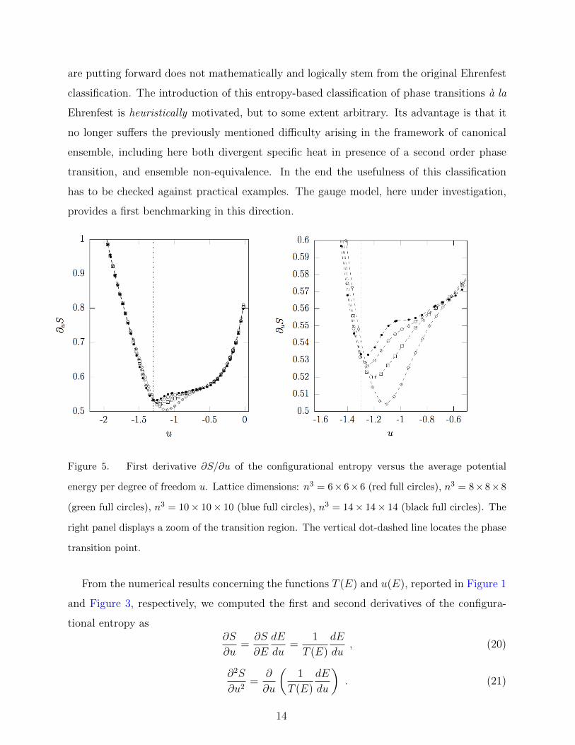
Figure 5. First derivative ∂S/∂u of the configurational entropy versus the average potential
energy per degree of freedom u. Lattice dimensions: n3 = 6×6×6 (red full circles), n3 = 8×8×8
(green full circles), n3 = 10× 10× 10 (blue full circles), n3 = 14× 14× 14 (black full circles). The
right panel displays a zoom of the transition region. The vertical dot-dashed line locates the phase
transition point.
From the numerical results concerning the functions T (E) and u(E), reported in Figure 1
and Figure 3, respectively, we computed the first and second derivatives of the configura-
tional entropy as∂S
∂u=∂S
∂E
dE
du=
1
T (E)
dE
du, (20)
∂2S
∂u2=
∂
∂u
(1
T (E)
dE
du
). (21)
14

-0.8
-0.6
-0.4
-0.2
0
0.2
-1.8 -1.6 -1.4 -1.2 -1 -0.8 -0.6 -0.4
∂2 uS
u
Figure 6. Second derivative ∂2S/∂u2 of the configurational entropy versus the average potential
energy per degree of freedom u. Lattice dimensions: n3 = 6 × 6 × 6 (rhombs), n3 = 8 × 8 × 8
(squares), n3 = 10× 10× 10 (circles), n3 = 14× 14× 14 (full circles). The vertical dot-dashed line
locates the phase transition point.
The derivative (dE/du) entering Eq.(20) is obtained after inversion of the function u = u(E)
reported in Figure 3 and by means of a spline interpolation of its points. Whereas ∂2uS(u)
in Eq.(21) is computed from the raw numerical data, and the derivatives with respect to u
have been obtained by means of a standard central difference formula.
The four patterns of ∂uS(u), computed for different sizes of the lattice and reported
in Figure 5, show that each ∂uS(u) appears splitted into two monotonic branches, one
decreasing and the other increasing as functions of u, respectively. Approximately out of
the interval u ∈ (−1.6,−0.65) the four patterns are perfectly superposed, whereas within this
interval - which contains the transition value uc ' −1.32 - we can observe that the transition
from ∂uS < 0 to ∂uS > 0 gets sharper at increasing lattice dimension. This means that
the second derivative of the entropy, ∂2uS(u), tends to make a sharper jump at increasing
N . And in fact, this is what is suggested by the four patterns of ∂2uS(u) - computed for
the same sizes of the lattice - reported in Figure 6. These are strongly suggestive to belong
to a sequence of patterns converging to a step-like limit pattern. In this case the third
15
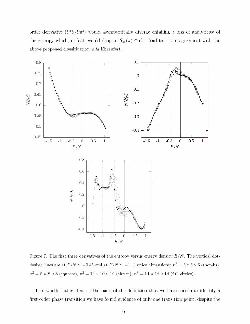
order derivative (∂3S/∂u3) would asymptotically diverge entailing a loss of analyticity of
the entropy which, in fact, would drop to S∞(u) ∈ C1. And this is in agreement with the
above proposed classification a la Ehrenfest.
0.45
0.5
0.55
0.6
0.65
0.7
0.75
0.8
-1.5 -1 -0.5 0 0.5 1
N∂ES
E/N
-0.4
-0.2
0
0.2
0.4
0.6
0.8
-1.5 -1 -0.5 0 0.5 1
N3∂3 ES
E/N
Figure 7. The first three derivatives of the entropy versus energy density E/N . The vertical dot-
dashed lines are at E/N ' −0.45 and at E/N ' −1. Lattice dimensions: n3 = 6× 6× 6 (rhombs),
n3 = 8× 8× 8 (squares), n3 = 10× 10× 10 (circles), n3 = 14× 14× 14 (full circles).
It is worth noting that on the basis of the definition that we have chosen to identify a
first order phase transition we have found evidence of only one transition point, despite the
16
presence of two peaks of the specific heat. In fact, only the first peak appears to be related
with the tendency to develop a loss of analyticity of the entropy with increasing N . At first
sight this is somewhat surprising, but this fact can be understood in the light of Ref.[35] and
hence by considering the energy dependence of (∂2S/∂E2), reported in Figure 7. Consider
the first point where (∂2S/∂E2) = 0, at E/N ' −1.3, here we have also (∂S/∂E) > 0 and
(∂3S/∂E3) > 0 so that, according to the classification given in [35], this corresponds to an
independent first order transition point, whereas at the second point where (∂2S/∂E2) = 0,
that is at E/N ' 0.3, we have (∂3S/∂E3) < 0 and still (∂S/∂E) > 0 so that this point
does not correspond to any kind of phase transition; for this to happen, the first derivative
of the entropy had to be negative. In Figure 7 we can identify two other inflection points of
the entropy, one is located at E/N ' −1 for which the third derivative of the entropy has
a positive minimum, that is, (∂3S/∂E3) > 0, (∂4S/∂E4) = 0, and (∂5S/∂E5) > 0, which
corresponds to an independent third order phase transition. This is a soft transition for
which we cannot identify any specific feature in the observables reported in Figures 1,2 and
3, the only clue that we could cautiously recognize in Figure 4, around E/N ' −1, is that
here the largest Lyapunov exponent starts to increase. As far as the second inflection point
at E/N ' 0.75 is concerned, we can see in Figure 7 that (∂3S/∂E3) < 0, (∂4S/∂E4) = 0, and
(∂5S/∂E5) > 0, and, according to Ref.[35], this does not correspond to any phase transition
point.
Remarkably, for the system that we are considering in the present work which has a
thermodynamic limit, the first order independent phase transition point corresponds to an
asymptotic loss of analyticity of the entropy. It will be worth to further investigate this point
in order to figure out whether, for example, this could make a difference between depen-
dent and independent transition points, that is, if independent phase transition points are
associated with singularities of the entropy, of course for systems having a thermodynamic
limit.
D. A geometric observable for the level sets Σv in configuration space
We have seen in the preceding Section that - within the confidence limits of a numer-
ical investigation - the first order phase transition of the gauge model under investigation
seems to correspond to an asymptotic divergence of the third derivative (∂3S/∂u3) of the
17
microcanonical configurational entropy. The question now is whether this fact can be the
“shadow” of a deeper phenomenon, that is, of the occurrence of some major and suitable
change of geometrical - and possibly also topological - properties of some subspaces of
the configuration space associated with the model. More precisely, and along a geomet-
rical/topological approach already put forward in recent years and summarised in Ref.[7],
the relevant information about the appearance of a phase transition in a physical system is
already encoded into peculiar changes with v of the geometry and topology of the members
of the family of level sets VN(q1, . . . , qN) = v ∈ R of its potential function V (q1, . . . , qN),
equivalently denoted by ΣNv = V −1
N (v), which are hypersurfaces of configuration space.
Constructively, relevant geometric quantities can be computed through the extrinsic ge-
ometry of hypersurfaces of a Euclidean space. To do this one has to study the way in which
an N -surface Σ curves around in RN+1 by measuring the way the normal direction changes
as we move from point to point on the surface. The rate of change of the normal direction
N at a point x ∈ Σ in direction v is described by the shape operator (sometimes also called
Weingarten’s map) Lx(v) = −∇vN = −(v · ∇)N, where v is a tangent vector at x and ∇v
is the directional derivative; gradients and vectors being represented in RN+1.
For the level sets of a regular function, as is the case of the constant-energy hypersurfaces
in the phase space of Hamiltonian systems or of the equipotential hypersurfaces in configura-
tion space, thus generically defined through a regular real-valued function f as Σa := f−1(a),
the normal vector is N = ∇f/‖∇f‖. The eigenvalues κ1(x), . . . , κN(x) of the shape operator
are the principal curvatures at x ∈ Σ. For the potential level sets Σv = V −1(v) the trace
of the shape operator at any given point is the mean curvature at that point and can be
written as [7, 36]
M = − 1
N∇ ·(∇V‖∇V ‖
)=
1
N
N∑i=1
κi . (22)
We have numerically computed the second moment of M averaged along the Hamiltonian
flow
σM = N〈V ar(M)〉t = N [〈M2〉t − 〈M〉2t ] '1
N
N∑i=1
〈κ2i 〉t −
1
N
N∑i=1
〈κi〉2t , (23)
where we have assumed that the correlation term N−2∑
i,j[〈kikj〉t − 〈ki〉t〈kj〉t] vanishes. In
fact, on the one side there is no conserved ordering of the eigenvalues of the shape operator
along a dynamical trajectory, and on the other side the averages are performed along chaotic
trajectories (the largest Lyapounov exponent is always positive) so that ki and kj vary almost
18
randomly from point to point and independently one from the other.
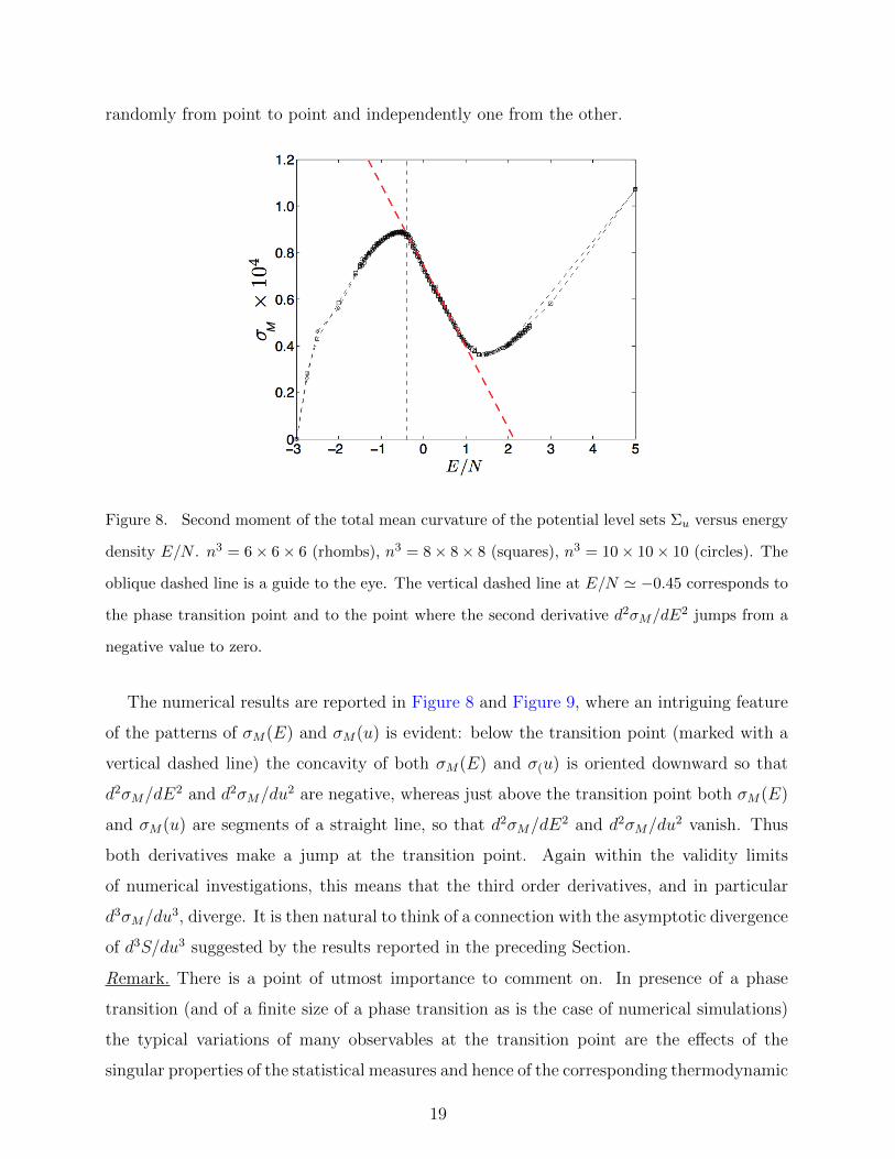
Figure 8. Second moment of the total mean curvature of the potential level sets Σu versus energy
density E/N . n3 = 6× 6× 6 (rhombs), n3 = 8× 8× 8 (squares), n3 = 10× 10× 10 (circles). The
oblique dashed line is a guide to the eye. The vertical dashed line at E/N ' −0.45 corresponds to
the phase transition point and to the point where the second derivative d2σM/dE2 jumps from a
negative value to zero.
The numerical results are reported in Figure 8 and Figure 9, where an intriguing feature
of the patterns of σM(E) and σM(u) is evident: below the transition point (marked with a
vertical dashed line) the concavity of both σM(E) and σ(u) is oriented downward so that
d2σM/dE2 and d2σM/du
2 are negative, whereas just above the transition point both σM(E)
and σM(u) are segments of a straight line, so that d2σM/dE2 and d2σM/du
2 vanish. Thus
both derivatives make a jump at the transition point. Again within the validity limits
of numerical investigations, this means that the third order derivatives, and in particular
d3σM/du3, diverge. It is then natural to think of a connection with the asymptotic divergence
of d3S/du3 suggested by the results reported in the preceding Section.
Remark. There is a point of utmost importance to comment on. In presence of a phase
transition (and of a finite size of a phase transition as is the case of numerical simulations)
the typical variations of many observables at the transition point are the effects of the
singular properties of the statistical measures and hence of the corresponding thermodynamic
19
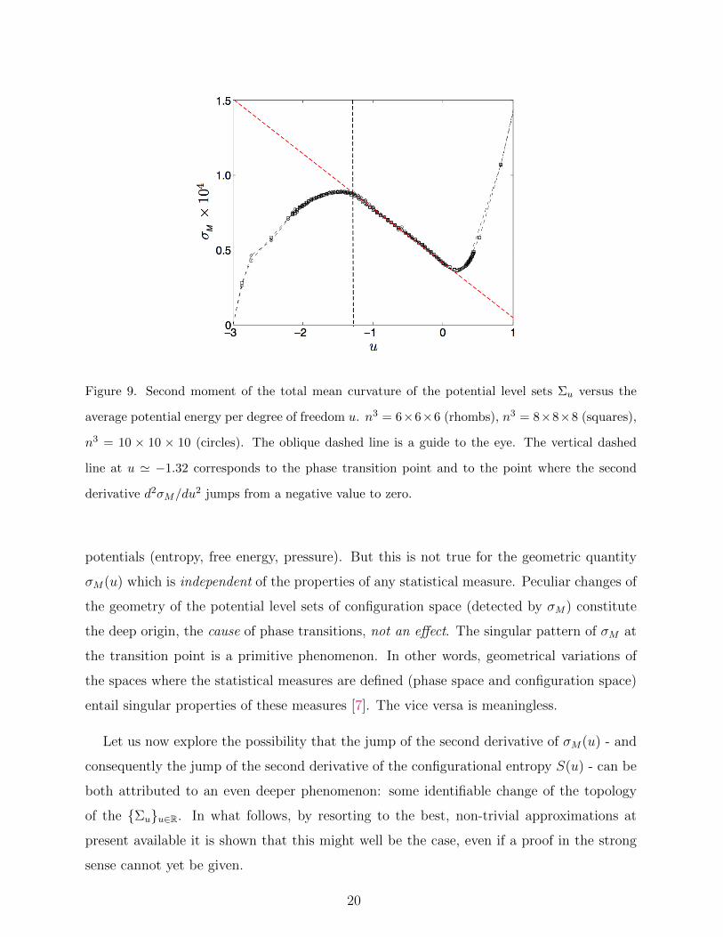
Figure 9. Second moment of the total mean curvature of the potential level sets Σu versus the
average potential energy per degree of freedom u. n3 = 6×6×6 (rhombs), n3 = 8×8×8 (squares),
n3 = 10 × 10 × 10 (circles). The oblique dashed line is a guide to the eye. The vertical dashed
line at u ' −1.32 corresponds to the phase transition point and to the point where the second
derivative d2σM/du2 jumps from a negative value to zero.
potentials (entropy, free energy, pressure). But this is not true for the geometric quantity
σM(u) which is independent of the properties of any statistical measure. Peculiar changes of
the geometry of the potential level sets of configuration space (detected by σM) constitute
the deep origin, the cause of phase transitions, not an effect. The singular pattern of σM at
the transition point is a primitive phenomenon. In other words, geometrical variations of
the spaces where the statistical measures are defined (phase space and configuration space)
entail singular properties of these measures [7]. The vice versa is meaningless.
Let us now explore the possibility that the jump of the second derivative of σM(u) - and
consequently the jump of the second derivative of the configurational entropy S(u) - can be
both attributed to an even deeper phenomenon: some identifiable change of the topology
of the Σuu∈R. In what follows, by resorting to the best, non-trivial approximations at
present available it is shown that this might well be the case, even if a proof in the strong
sense cannot yet be given.
20
Consider the pointwise dispersion of the principal curvatures
sκ =1
N
N∑i=1
(κi − κ)2 (24)
where
κ =1
N
N∑i=1
κi (25)
equation (24) is equivalently rewritten as [37]
sκ =1
N2
N∑i,j=1
(κi − κj)2 (26)
and the time average along the Hamiltonian flow of sκ is then equivalently written as
〈sκ〉t =1
N
N∑i=1
〈κ2i 〉t − 〈κ2〉t =
1
N2
N∑i,j=1
〈(κi − κj)2〉t . (27)
Now, from Eqs.(23) and (27) we get
σM − 〈sκ〉t ' −1
N
N∑i=1
〈κi〉2t + 〈κ2〉t (28)
so that, based on the empirical/numerical observation that at large N the potential level
sets locally appear as of almost constant curvature, that is, locally isotropic, we make a
“quasi isotropy” assumption which is equivalent to replace the κi with their average κ in
the first term of the r.h.s. of (28), hence it follows σM − 〈sκ〉t ' −〈κ〉2t + 〈κ2〉t, and as κ in
Eq.(25) is the same of M in Eq.(22) one trivially gets
(1− 1
N)σM − 〈sκ〉t ' 0 (29)
so that, under this “quasi isotropy” assumption, σM in Eq.(23) can be used to estimate
〈sκ〉t. Then, as the ergodic invariant measure of chaotic Hamiltonian dynamics is the micro-
canonical one, the time averages 〈·〉t provide the values of the surface averages 〈·〉ΣE . Hence,
and within the validity limits of the undertaken approximations, an interesting connection
can be used between extrinsic curvature properties of an hypersurface of a Euclidean space
RN+1 and its Betti numbers (the diffeomorphism-invariant dimensions of the cohomology
groups of the hypersurface, thus topological invariants) [38]. This connection is made by
Pinkall’s inequality given in the following.
21
Denoting by
σ(Lx)2 =
1
N2
∑i<j
(κi − κj)2
the dispersion of the principal curvatures of the hypersurface, then after Pinkall’s theorem
[39]
1
vol(SN)
∫ΣNv
[σ(Lx)]N dµ(x) ≥
N−1∑i=1
(i
N − i
)N/2−ibi(Σ
Nv ) , (30)
where bi(ΣNv ) are the Betti numbers of the manifold ΣN
v immersed in the Euclidean space
RN+1, SN is an N -dimensional sphere of unit radius, and µ(x) is the measure on ΣNv .
With the help of the Holder inequality for integrals we have∫ΣNv
[σ(Lx)]2 dµ(x) ≤
[∫ΣNv
[σ(Lx)]2N/2dµ(x)
]2/N [∫ΣNv
dµ(x)
]1/(1−2/N)
(31)
whence, at large N ,[∫ΣNv
dµ(x)
]−1 ∫ΣNv
[σ(Lx)]2 dµ(x) ≤
[∫ΣNv
[σ(Lx)]2N/2dµ(x)
]2/N
(32)
this inequality becomes an equality when |f |p/‖f‖pp = |g|q/‖g‖qq almost everywhere [40],
where ‖f‖p is the standard Lp norm ‖f‖p =(∫
S|f |pdµ(x)
)1/p, where S is a measurable space.
In the inequalities above g(x) = 1, thus the Holder inequality becomes an equality when
|f |p = ‖f‖pp/∫Sdµ(x), that is, when |σ(Lx)|N equals its average value almost everywhere on
ΣNv . Introducing a positive remainder function r(v), Eq.(32) is rewritten as[∫
ΣNv
dµ(x)
]−1 ∫ΣNv
[σ(Lx)]2 dµ(x) =
[∫ΣNv
[σ(Lx)]2N/2dµ(x)
]2/N
− r(v) . (33)
For the model under investigation, the pointwise dispersion of the principal curvatures of
the potential level sets actually displays a limited variability from point to point. This fol-
lows from the observation that the numerically computed variance of the mean curvature in
Eq.(23) is very fastly convergent to its asymptotic value, independently of the initial condi-
tion. The spread of the values of σM = N〈V ar(M)〉∆t = N [〈M2〉∆t − 〈M〉2∆t], numerically
computed along short segments of time duration ∆t = 100, out of long phase space trajecto-
ries - of a time duration of t = 106 - typically amounts to 3− 5%. As a consequence, on this
slightly coarse-grained manifold the condition to make Holder inequality an equality is not
far from being satisfied, what indicates that in the case under study the Holder inequality
is reasonably tight and the remainder r(v) can be considered as a small correction.
22
Then, using
σM = N [〈M2〉Σv − 〈M〉2Σv ] ∼[∫
ΣNv
dµ(x)
]−1 ∫Σv
[σ(Lx)]2 dµ(x) (34)
together with Eq.(33) and the Pinkall inequality, one finally gets
σM ∼[∫
ΣNv
[σ(Lx)]2N/2dµ(x)
]2/N
−r(v) ∼
[vol(SN)
N−1∑i=1
(i
N − i
)N/2−ibi(Σ
Nv )
]2/N
−r(v) ,
(35)
that is, the observable σM(v) is explicitly related with the topology of the level sets ΣNv . This
relation, even being an approximate one, is definitely non-trivial because there are very few
possibilities of relating total curvature properties of a manifold with its topological invariants.
On the other hand, both Pinkall’s inequality and the Holder inequality are sufficiently tight
to make Eq.(35) meaningful. In fact, in addition to the already given arguments concerning
the Holder inequality in Eq.(32), Pinkall’s inequality stems from the Morse inequalities
µk(M) ≥ bk(M) which relate the Morse indexes µk(M) to the Betti numbers bk(M) of a
manifold M (Pinkall’s inequality would be replaced by an equality if written with Morse
indexes), and these Morse inequalities are very tight since the alternating sums of Morse
indexes and of Betti numbers, respectively, give the same result (the Euler characteristic).
Therefore, the integral in the l.h.s. of Eq.(35) necessarily follows the topological variations
of the ΣNv described by the weighted sum of its Betti numbers. The consequence is that
a suitable variation with v of the weighted sum of the Betti numbers of a ΣNv can be
sufficient to entail a sudden change of the convexity of the function σM(v), as reported in
Figure 9, and thus entail a discontinuity of its second derivative [41]. Sufficiency means
that independently of r(v), if some sharp change of the topology of the ΣNv takes place, then
σM(v) is affected.
On the other hand, the existence of a relationship between thermodynamics and config-
uration space topology is provided by the following exact formula [7, 19]
S(−)N (v) = (kB/N) log
[∫MNv
dNq
]
=kBN
log
vol[MNv \
N (v)⋃i=1
Γ(x(i)c )] +
N∑i=0
wi µi(MNv ) +R
, (36)
where S(−)N is the configurational entropy, and the µi(M
Nv ) are the Morse indexes (in one-to-
one correspondence with topology changes) of the submanifolds MNv = V −1
N ((−∞, v])v∈R
23
of configuration space; in square brackets: the first term is the result of the excision of certain
neighbourhoods of the critical points of the interaction potential from MNv ; the second term
is a weighed sum of the Morse indexes, and the third term is a smooth function of N and v.
Again, sharp changes in the potential energy pattern of at least some of the µi(MNv ) (thus
of the way topology changes with v) affect S(−)N (v) and its derivatives.
In other words, both the jump of the second derivative of the entropy and of the second
derivative of σM are possibly rooted in the same topological ground, where some adequate
variation of the topology of the ΣNv - foliating the configuration space - takes place. Notice
that even if in Eq.(36) S(−)N (v) depends on the topology of the MN
v through the Morse
indexes µi(MNv ), in the framework of Morse theory a topology change of a level set ΣN
v is
always associated with a topology change of the associated manifold MNv of which ΣN
v is the
boundary [42].
Summarizing, the topology changes which seem to be indirectly detected by the func-
tion σM(u) can affect the configurational entropy SN(v) and its tendency to develop an
asymptotic discontinuity of ∂2vS∞(v) (we use u and v interchangeably). Notice that directly
computing the Betti numbers of the ΣNv , or of the MN
v , is in general undoable. In some
very special cases [13, 14] it has been possible to analytically compute the Morse indexes of
these manifolds, which are good estimators of the Betti numbers. But in general one has to
necessarily resort to known results in differential topology relating total curvature proper-
ties of a manifold with its topological invariants. This is the case of the Gauss-Bonnet-Hopf
theorem for hypersurfaces of N -dimensional Euclidean spaces, where the integral of the
Gauss-Kronecker curvature is proportional to the Euler characteristic of the hypersurface,
of the Chern-Lashof theorem where the integral of the modulus of the Gauss-Kronecker cur-
vature gives the sum of the Morse indexes of the manifold, or the Pinkall theorem which has
been used in the present work. And, in general, we can wonder how to combine Ehrenfest’s
classification of phase transitions in the microcanonical configuration space, put forward in
Section III.C, with the topological transitions in the absence of an order parameter, for in-
stance, we can wonder how the present analysis of a first order transition without symmetry
breaking would work in the case of second order transitions without symmetry breaking. In
this case, Eqs. (36) and (37) qualitatively indicate that suitable variations with v of the
µi(MNv ), or with E of the bi(ΣN
E ), can entail singular behaviors of any desired derivative
of the entropy. For a second order transition a discontinuity of the third derivative of the
24
entropy is required, but, again, this can be related to topology only through some theorem
of differential topology, thus through the energy variation of total geometric quantities.
Finally, in Appendix we give a more technical account of how the non-trivial contribution
to the homology groups of the energy level sets ΣNE comes from the homology groups of the
configuration space submanifolds MNv ⊂ MN
E and ΣNv ⊂ ΣN
E . Therefore, the topology
variations of the ΣNv imply topology variations of the ΣN
E , and these necessarily affect also
the functional dependence on E of the total entropy SN(E). In fact, the variation with v of
the topology of the ΣNv is in one-to-one correspondence with some variation with v of the
Betti numbers bi(ΣNv ) entering Eq.(35), and this entails the variation with E of the Betti
numbers bi(ΣNE ), so that, according to the following formula [7] for the total entropy
SN(E) ≈ kB
Nlog
[vol(SN−1
1 )N∑i=0
bi(ΣNE ) +R1(E)
]+R2(E) , (37)
where R1(E), and R2(E) are smooth functions, we see that the variation with v of the
topology of the ΣNv implies also the variation with E of the total entropy.
IV. CONCLUDING REMARKS
We have tackled the problem of characterizing a phase transition in the absence of global
symmetry breaking from the point of view of Hamiltonian dynamics and related geometri-
cal and topological aspects. In this condition the Landau classification of phase transitions
does not apply, because no order parameter - commonly associated with a global symmetry
- exists. The system chosen is inspired by the dual of the Ising model, and the discrete
variables are replaced by continuous ones. We stress that our work has nothing to do with
the true dual Ising model, which has just suggested how to define a classical Hamiltonian
system with a local (gauge) symmetry. Since the ergodic invariant measure for generically
non-integrable Hamiltonian systems is the microcanonical measure in phase space, study-
ing phase transitions through Hamiltonian dynamics is the same as studying them in the
microcanonical ensemble.
A standard analysis has been performed to locate the phase transition and to determine
its order through the shape of the caloric curve, T = T (E), which appeared typical of
a first order phase transition. The presence of energy intervals of negative specific heat
are indicative of ensemble nonequivalence. At variance with what has been systematically
25
observed for systems undergoing symmetry-breaking phase transitions, the energy pattern
of the largest Lyapunov exponent does not allow to locate the transition point.
After the Yang-Lee theory, phase transitions are commonly associated with a loss of an-
alyticity of a thermodynamic potential entailing non-analytic patterns of thermodynamic
observables (the pertinent potential depends on the statistical ensemble chosen). However,
there is no evidence of the existence of genuinely non-analytic energy pattern of some ob-
servable for our gauge model, in fact, no bifurcating order parameter exists, the caloric curve
is a regular function, and the peaks of the specific heat are just due to horizontal tangencies
to the caloric curve and a-priori are not necessarily due to singularities of the entropy. Nev-
ertheless, an analyticity loss of the entropy has been directly detected through a point of
discontinuity of the second derivative of the entropy (or at least a finite size version of such
a discontinuity), thus an asymptotic divergence of its third derivative. As a consequence,
this fits properly into the classification scheme a la Ehrenfest discussed in Section III.C
for the microcanonical ensemble. Then, by resorting to the classification of microcanonical
phase transitions based on inflection-point analysis of Ref.[35] we have been able to inter-
estingly complement the interpretation of our numerical outcomes for the thermodynamic
observables.
Remarkably, we have found a quantity, σM(v), that - by measuring the total degree
of inhomogeneity of the extrinsic curvature of the potential level sets Σv = V −1(v) in
configuration space - identifies the phase transition point. This quantity is not a ther-
modynamic observable, has a purely geometric meaning, and displays a discontinuity of
its second derivative in coincidence with the same kind of discontinuity displayed by the
entropy. Rather than being a trivial consequence of the presence of the phase transition,
the peculiar change of the geometry of the ΣNv v∈R so detected is the deep cause of the
singularity of the entropy. In fact, the potential level sets are simply subsets of RN defined
as ΣNv = (q1, . . . , qN) ∈ RN |V (q1, . . . , qN) = v, whose ensemble ΣN
v v∈R foliates the con-
figuration space; the volume Ω(v,N) - of each leaf ΣNv - and the way it varies as a function
of v is just a matter of geometrical/topological properties of the leaves of the foliation.
These properties entail the v-dependence of the entropy SN(v) = (1/N) log Ω(v,N), and,
of course, its differentiability class. This is why the v-pattern of the quantity σM(v) is not
the consequence of the presence of a phase transition but, rather, the reason of its appear-
ance. This is already a highly non trivial fact indicating that whether a physical system
26
can undergo a phase transition is somehow already encoded in the interactions among its
degrees of freedom described by the potential function V (q1, . . . , qN), independently of the
statistical ensemble chosen to describe its macroscopic observables. However, we can wonder
if one can go deeper by looking for the origin of the peculiar changes with v of the geometry
of the ΣNv . Actually, by resorting to a theorem in differential topology, and with some ap-
proximations, these geometrical changes are strongly suggestive of the presence of changes
of the topology of both the potential level sets in configuration space and the energy level
sets in phase space. Therefore, although one single example cannot be taken as a rule, and
certainly much work remains to be done, the results of the present work go in the direction
of supporting the topological theory of phase transitions.
Moreover, since the practical computation of σM(v), or of σM(E), is rather straightfor-
ward, this can be used to complement the study of transitional phenomena in the absence of
symmetry-breaking, as is the case of: liquid-gas change of state, Kosterlitz-Thouless transi-
tions, glasses and supercooled liquids, amorphous and disordered systems, folding transitions
in homopolymers and proteins, both classical and quantum transitions in small N systems.
With respect to the latter case, a remark about the geometrical/topological theory is in
order. In nature, phase transitions (that is major qualitative physical changes) occur also in
very small systems with N much smaller than the Avogadro number, but their mathemat-
ical description through the loss of analyticity of thermodynamic observables requires the
asymptotic limit N →∞. To the contrary, within the geometrical/topological framework a
sharp difference between the presence or the absence of a phase transition can be made also
at any finite and even very small N . At finite N , the microscopic states that significantly
contribute to the statistical averages of thermodynamic observables are spread in regions
of configuration space which get narrower as N increases, so that the statistical measures
better concentrate on a specific potential level set thus better detecting its sudden and ma-
jor geometry and topology changes, if any. Eventually, in the N → ∞ limit the extreme
sharpening of the effective support of the measure leads to a geometry-induced, and possibly
also a topology-induced, nonanalyticity of thermodynamic observables [7].
Furthermore, even if somewhat abstract, the model studied in the present work has the
basic properties of a lattice gauge model, that is, its potential depends on the circulations
of the gauge field on the plaquettes, so that the geometrical/topological approach developed
here could be also of some interest to the numerical investigation of phase transitions of
27
Euclidean gauge theories on lattice. In fact, computing σM(v), or σM(E), is definitely much
easier than computing the Wilson loop, commonly adopted in place of an order parameter
for gauge theories. Actually, a few decades ago, several papers on the microcanonical formu-
lation of quantum field theories appeared [43, 44], motivated by the fact that in statistical
mechanics and in field theory there are systems for which the canonical description is patho-
logical, but the microcanonical is not, also arguing, for instance and among other things, that
a microcanonical formulation of quantum gravity may be less pathological than the usual
canonical formulation [45–48]. More recent works can also be found on these topics [49–52].
Moreover, in quantum many-body systems at zero temperature quantum phase transitions
can occur by varying some parameter of the Hamiltonian of the system. The different phases
correspond to qualitatively different quantum states which are not characterized by an order
parameter [53, 54] but rather described by suitably defined topological order. These topo-
logical phase transitions, occurring in the absence of symmetry breaking, are investigated
by resorting to the methods of quantum field theory [55]. Among the other topics, attention
has been given to the possible existence of second order phase transitions in the absence of
symmetry breaking, thus in the absence of an order parameter. Such a possibility, just to
give an example, has been suggested for the case of the deconfining transition of SU(N)
gauge theories in 2+1 dimensions for N ≤ 3 [56]. It is worth mentioning that, in princi-
ple, the topological approach to classical phase transitions - addressed in the present work
- and the just mentioned topological treatment of quantum transitions could be linked by
Wick’s analytic prolongation to imaginary times of the path-integral generating functional
of quantum field theory, this allows to map a quantum system onto a formally classical one
described by a classical partition function written with the euclidean Lagrangian action, on
lattice to have a countable number of degrees of freedom [7].
Finally, as a side issue, it is provided here an example of statistical ensemble non-
equivalence in a system with short-range interactions. Ensemble non-equivalence is another
topic which is being given much attention in recent literature [57].
28
APPENDIX
A. Relation between topological changes of the Σv and of the ΣE
Now, let us see why a topological change of the configuration space submanifolds Σv =
V −1(v) (potential level sets) implies the same phenomenon for the ΣE. The potential level
sets are the basic objects, foliating configuration space, that represent the nontrivial topo-
logical part of phase space. The link of these geometric objects with microcanonical entropy
is given by
S(−)(E) =kB2N
log
∫ E
0
dη
∫dNp δ(
∑i
p2i /2− η)
∫ΣE−η
dσ
‖∇V ‖. (38)
As N increases the microscopic configurations giving a relevant contribution to the entropy,
and to any microcanonical average, concentrate closer and closer on the level set Σ〈E−η〉. A
link among the topology of the energy level sets and the topology of configuration space can
be established for systems described by a Hamiltonian of the form HN(p, q) =∑N
i=1 p2i /2 +
VN(q1, ..., qN).
In fact, (using a cumbersome notation for the sake of clarity) the level sets ΣHNE of the
energy function HN can be given by the disjoint union of a trivial unitary sphere bundle
(representing the phase space region where the kinetic energy does not vanish) and the
hypersurface in configuration space where the potential energy takes the total energy value
(details are given in [? ])
ΣHNE homeomorphic to MVNE × SN−1
⊔ΣVNE (39)
where Sn is the n-dimensional unitary sphere and
M fc = x ∈ Dom(f)|f(x) < c ,
Σfc = x ∈ Dom(f)|f(x) = c .
(40)
The idea that finite N topology, and ”asymptotic topology” as well, of ΣHNE is affected by
the topology of the accessible region of configuration space is suggested by the Kunneth
formula: if Hk(X) is the k-th homological group of the topological space X on the field F
then
Hk(X × Y ;F) '⊕i+j=k
Hi(X;F) ⊗ Hj(Y ;F) . (41)
29
Moreover, as Hk
(tNi=1Xi,F
)=⊕N
i Hk(Xi,F), it follows that:
Hk
(ΣHNE ,R
)'⊕i+j=k
Hi
(MVN
E ;R)⊗ Hj
(SN−1;R
)⊕Hk
(ΣVNE ;R
)' Hk−(N−1)
(MVN
E ;R)⊗ R⊕Hk
(MVN
E ;R)⊗ R
⊕Hk
(ΣVNE ;R
)(42)
the r.h.s. of Eq.(42) shows that the topological changes of ΣHNE only stem from the topo-
logical changes in configuration space.
ACKNOWLEDGMENTS
The authors acknowledge the financial support of the Future and Emerging Technologies
(FET) Program within the Seventh Framework Program (FP7) for Research of the European
Commission, under the FET-Proactive TOPDRIM Grant No. FP7-ICT-318121. The project
leading to this publication has received funding also from the Excellence Initiative of Aix-
Marseille University - A*Midex, a French “Investissements d’Avenir” programme. Cecilia
Clementi acknowledges support by the National Science Foundation (CHE-1265929, CHE-
1738990, and PHY-1427654), the Welch Foundation (C-1570), and the Einstein Foundation
in Berlin.
[1] Part of this work was done while M.P. was on leave of absence from Osservatorio Astrofisico
di Arcetri, Florence, Italy.
[2] C.N. Yang, and T.D. Lee, Statistical theory of equations of state and phase transitions I.
Theory of condensation, Phys. Rev. 87, 404 - 409 (1952); T.D. Lee, and C.N. Yang, Statistical
theory of equations of state and phase transitions II. Lattice gas and Ising model, Phys. Rev.
87, 410 - 419 (1952).
[3] A comprehensive account of the Dobrushin-Lanford-Ruelle theory and of its developments
can be found in: H.O. Georgii, Gibbs Measures and Phase Transitions, Second Edition, (De
Gruyter, Berlin 2011).
30
[4] D.H.E. Gross, Microcanonical Thermodynamics. Phase Transitions in “Small” Systems,
(World Scientific, Singapore, 2001).
[5] M. Bachmann, Thermodynamics and Statistical Mechanics of Macromolecular Systems, (Cam-
bridge University Press, New York, 2014).
[6] Ph. Chomaz, V. Duflot, and F. Gulminelli, Caloric Curves and Energy Fluctuations in the
Microcanonical Liquid-Gas Phase Transition, Phys. Rev. Lett. 85, 3587 - 3590 (2000).
[7] M. Pettini, Geometry and Topology in Hamiltonian Dynamics and Statistical Mechanics, IAM
Series n.33, (Springer, New York, 2007).
[8] L. Casetti, M. Cerruti-Sola, M. Modugno, G. Pettini, M. Pettini and R. Gatto, Dynamical
and Statistical properties of Hamiltonian systems with many degrees of freedom, Rivista del
Nuovo Cimento 22, 1-74 (1999), and references quoted therein.
[9] L.Casetti, M. Pettini, E.G.D. Cohen, Geometric approach to Hamiltonian dynamics and sta-
tistical mechanics, Phys. Rep. 337, 237-342 (2000), and references quoted therein.
[10] M. Pettini, Geometrical hints for a nonperturbative approach to Hamiltonian dynamics, Phys.
Rev. E 47, 828 (1993).
[11] L. Casetti, E.G.D. Cohen, and M. Pettini, Topological origin of the phase transition in a
mean-field model, Phys. Rev. Lett. 82, 4160 (1999).
[12] L. Casetti, E.G.D. Cohen, and M. Pettini, Exact result on topology and phase transitions at
any finite N , Phys. Rev. E 65, 036112 (2002).
[13] L. Casetti, M. Pettini and E.G.D. Cohen, Phase transitions and topology changes in configu-
ration space, J. Stat. Phys. 111, 1091 (2003).
[14] L. Angelani, L. Casetti, M. Pettini, G. Ruocco, and F. Zamponi, Topology and Phase Tran-
sitions: from an exactly solvable model to a relation between topology and thermodynamics,
Phys. Rev. E71, 036152 (2005).
[15] F. A. N. Santos, L. C. B. da Silva, and M. D. Coutinho-Filho, Topological approach to
microcanonical thermodynamics and phase transition of interacting classical spins, J. Stat.
Mech. 2017, 013202 (2017).
[16] Even though a counterexample was given in: M. Kastner and D. Mehta, Phase Transitions
Detached from Stationary Points of the Energy Landscape, Phys. Rev. Lett. 107, 160602
(2011), the problem can be fixed with a refinement of the hypotheses of the theorems, as
shown in: M. Gori, R. Franzosi, and M. Pettini, Toward a refining of the topological theory
31
of phase transitions, arXiv:1706.01430 [cond-mat.stat-mech].
[17] R. Franzosi, and M. Pettini, Theorem on the origin of Phase Transitions, Phys. Rev. Lett. 92,
060601 (2004).
[18] R. Franzosi, M. Pettini, and L. Spinelli, Topology and Phase Transitions I. Preliminary results,
Nucl. Phys. B782 [PM], 189 (2007).
[19] R. Franzosi and M. Pettini, Topology and Phase Transitions II. Theorem on a necessary
relation, Nucl. Phys. B782 [PM], 219 (2007).
[20] J. Kogut, An introduction to lattice gauge theory and spin systems, Rev. Mod. Phys. 51, 659
(1979).
[21] S. Elitzur, Impossibility of Spontaneously Breaking Local Symmetries, Phys. Rev. D12, 3978
(1975).
[22] L. Casetti, Efficient symplectic algorithms for numerical simulations of Hamiltonian flows,
Physica Scripta 51, 29 (1995).
[23] E. M. Pearson, T. Halicioglu, and W.A. Tiller, Laplace-transform technique for deriving
thermodynamic equations from the classical microcanonical ensemble, Phys. Rev. A32, 3030
(1985).
[24] For generic quasi-integrable systems, in the form H(α, J) = H0(J) + εH1(α, J) with (α, J)
action-angle coordinates, with three or more degrees of freedom, after the Poincare-Fermi
theorem for any ε > 0 all the integrals of motion except the energy are destroyed, so that there
is no topological obstruction to ergodicity. On the other hand, a lack of ergodicity stemming
from KAM theorem requires exceedingly tiny values of the perturbation and ε < εc where
εc drops to zero more than exponentially with the number of degrees of freedom. Moreover,
generic nonintegrable systems are chaotic, so that, from the physicists’ viewpoint these systems
are bona fide ergodic and mixing.
[25] L. Caiani, L. Casetti, C. Clementi, and M. Pettini, Geometry of dynamics, Lyapunov expo-
nents and phase transitions, Phys. Rev. Lett. 79, 4361 (1997).
[26] V. Mehra, and R. Ramaswamy, Curvature fluctuations and the Lyapunov exponent at melting,
Phys. Rev. E 56, 2508 (1997).
[27] L. Caiani, L. Casetti, C. Clementi, G. Pettini, M. Pettini, and R. Gatto, Geometry of dynamics
and phase transitions in classical lattice ϕ4 theories, Phys. Rev. E 57, 3886 (1998).
[28] L. Caiani, L. Casetti and M. Pettini, Hamiltonian dynamics of the two-dimensional lattice ϕ4
32
model, J. Phys. A: Math. Gen. 31, 3357 (1998).
[29] M.-C. Firpo, Analytic estimation of the Lyapunov exponent in a mean-field model undergoing
a phase transition, Phys. Rev. E 57, 6599 (1998).
[30] J. Barre, and T. Dauxois, Lyapunov exponents as a dynamical indicator of a phase transition,
Europhys. Lett. 55, 164 (2001).
[31] S. Hilbert, and J. Dunkel, Nonanalytic microscopic phase transitions and temperature os-
cillations in the microcanonical ensemble: An exactly solvable one-dimensional model for
evaporation, Phys. Rev. E74, 011120 (2006).
[32] S. Schnabel, et al., Microcanonical entropy inflection points: Key to systematic understanding
of transitions in finite systems, Phys. Rev. E84, 011127 (2011).
[33] J. Lee, Microcanonical analysis of a finite-size nonequilibrium system, Phys. Rev. E93, 052148
(2016).
[34] P. Schierz, P. Zierenberg, and W. Janke, First-order phase transitions in the real microcanon-
ical ensemble, Phys. Rev. E94, 021301 (2016).
[35] K. Qi and M. Bachmann, Classification of Phase Transitions by Microcanonical Inflection-
Point Analysis, Phys. Rev. Lett. 120,180601 (2018).
[36] J.A. Thorpe, Elementary Topics in Differential Geometry, (Springer-Verlag, New York 1979).
[37] Y. Zhang, H. Wu, and L. Cheng, Some New Deformation Formulas about Variance and
Covariance, Proceedings of 4th International Conference on Modelling, Identification and
Control, Wuhan, China, June 24-26, (2012).
[38] M. Nakahara, Geometry, Topology and Physics, (Adam Hilger, Bristol, 1991).
[39] U. Pinkall, Inequalities of Willmore Type for Submanifolds, Math. Zeit. 193, 241 (1986).
[40] M. Reed, and B. Simon, vol. 1: Functional Analysis, revised and enlarged edition, (Academic
Press, San Diego, 1980).
[41] The Betti numbers - as well as Morse indexes - are integers so that their sum, weighted
or not, forms only staircase-like patterns which do not qualify as continuous and possibly
differentiable functions. Actually the technical details of the reason why the corners of these
staircase-like patterns are rounded can be found in Section 9.5 of Ref.[7].
[42] J. Milnor, Morse Theory, Ann. Math. Studies 51, (Princeton University Press, Princeton
1963).
[43] D.J.E. Callaway, and A. Rahman, Lattice gauge theory in the microcanonical ensemble, Phys.
33
Rev. D28, 1506 (1983).
[44] M. Fukugita,T. Kaneko, and A. Ukawa, Testing microcanonical simulation with SU(2) lattice
gauge theory, Nucl. Phys. B270 365 (1986).
[45] A. Strominger, Microcanonical Quantum Field Theory, Ann. Phys. NY 146, 419 (1983).
[46] A. Iwazaki, Microcanonical formulation of Quantum field theories, Phys. Lett. B141, 342
(1984).
[47] Y. Morikawa, and A. Iwazaki, Supercooled states and order of phase transitions in microcanon-
ical simulations, Phys. Lett. B165, 361 (1984).
[48] S. Duane, Stochastic quantization versus the microcanonical ensemble: getting the best of both
worlds, Nucl. Phys. B257 , 652 (1985).
[49] D.J. Cirilo-Lombardo, Quantum field propagator for extended-objects in the microcanonical
ensemble and the S-matrix formulation, Phys. Lett. B637, 133 (2006).
[50] R. Casadio, and B. Harms, Microcanonical Description of (Micro) Black Holes, Entropy 13,
502 (2011).
[51] A. Sinatra, and Y. Castin, Genuine phase diffusion of a Bose-Einstein condensate in the
microcanonical ensemble: A classical field study, Phys. Rev. A78, 05361 (2008).
[52] Y. Strauss, L. P. Horwitz, J. Levitan, and A. Yahalom, Quantum field theory of classically
unstable Hamiltonian dynamics, J. Math. Phys. 56, 072701 (2015).
[53] M. Levin and X.G. Wen, Detecting Topological Order in a Ground State Wave Function, Phys.
Rev. Lett. 96, 110405 (2006).
[54] A. Kitaev and J. Preskill, Topological Entanglement Entropy, Phys. Rev. Lett. 96, 110404
(2006).
[55] X.G. Wen, Quantum Field Theory of Many Body Systems, (Oxford University Press, Oxford
2007).
[56] J. Liddle and M. Teper, The deconfining phase transition in D=2+1 SU(N) gauge theories,
XXIII International Symposium on Lattice Field Theory, 25-30 July 2005, Trinity College,
Dublin, Ireland, in: Proceedings of Science (2005) 188.
[57] A. Campa, T. Dauxois, and S. Ruffo, Statistical mechanics and dynamics of solvable models
with long-range interactions, Phys. Rep. 480, 57 - 159 (2009).
34


![A STUDY OF PHASE TRANSITIONS IN CRYSTALUNE SOLIDS · 2018-01-04 · insight into the microscopic origin of structural phase transitions[9]. The study of vibrational properties help](https://img.pdfslide.net/doc/110x75/5f3b6de66200dc5fde281404/a-study-of-phase-transitions-in-crystalune-solids-2018-01-04-insight-into-the.jpg)