On the Practice of Dichotomization of Quantitative …€¦ · · 2010-05-28On the Practice of Dichotomization of Quantitative Variables ... The authors examine the practice of

On the Practice of Dichotomization of Quantitative Variables

Robert C. MacCallum, Shaobo Zhang, Kristopher J. Preacher, and Derek D. RuckerOhio State University

The authors examine the practice of dichotomization of quantitative measures,wherein relationships among variables are examined after 1 or more variables havebeen converted to dichotomous variables by splitting the sample at some point onthe scale(s) of measurement. A common form of dichotomization is the mediansplit, where the independent variable is split at the median to form high and lowgroups, which are then compared with respect to their means on the dependentvariable. The consequences of dichotomization for measurement and statisticalanalyses are illustrated and discussed. The use of dichotomization in practice isdescribed, and justifications that are offered for such usage are examined. Theauthors present the case that dichotomization is rarely defensible and often willyield misleading results.

We consider here some simple statistical proce-dures for studying relationships of one or more inde-pendent variables to one dependent variable, where allvariables are quantitative in nature and are measuredon meaningful numerical scales. Such measures areoften referred to asindividual-differences measures,meaning that observed values of such measures areinterpretable as reflecting individual differences onthe attribute of interest. It is of course straightforwardto analyze such data using correlational methods. Inthe case of a single independent variable, one can usesimple linear regression and/or obtain a simple corre-lation coefficient. In the case of multiple independentvariables, one can use multiple regression, possiblyincluding interaction terms. Such methods are rou-tinely used in practice.

However, another approach to analysis of such datais also rather widely used. Considering the case of oneindependent variable, many investigators begin byconverting that variable into a dichotomous variableby splitting the scale at some point and designatingindividuals above and below that point as defining

two separate groups. One common approach is to splitthe scale at the sample median, thereby defining highand low groups on the variable in question; this ap-proach is referred to as a median split. Alternatively,the scale may be split at some other point based on thedata (e.g., 1 standard deviation above the mean) or ata fixed point on the scale designated a priori. Re-searchers may dichotomize independent variables formany reasons—for example, because they believethere exist distinct groups of individuals or becausethey believe analyses or presentation of results will besimplified. After such dichotomization, the indepen-dent variable is treated as a categorical variable andstatistical tests then are carried out to determinewhether there is a significant difference in the mean ofthe dependent variable for the two groups representedby the dichotomized independent variable. Whenthere are two independent variables, researchers oftendichotomize both and then analyze effects on the de-pendent variable using analysis of variance(ANOVA).

There is a considerable methodological literatureexamining and demonstrating negative consequencesof dichotomization and firmly favoring the use of re-gression methods on undichotomized variables. Nev-ertheless, substantive researchers often dichotomizeindependent variables prior to conducting analyses. Inthis article we provide a thorough examination of thepractice of dichotomization. We begin with numericalexamples that illustrate some of the consequences ofdichotomization. These include loss of informationabout individual differences as well as havoc with

Robert C. MacCallum, Shaobo Zhang, Kristopher J.Preacher, and Derek D. Rucker, Department of Psychology,Ohio State University.

Shaobo Zhang is now at Fleet Credit Card Services, Hor-sham, Pennsylvania.

Correspondence concerning this article should be ad-dressed to Robert C. MacCallum, Department of Psychol-ogy, Ohio State University, 1885 Neil Avenue, Columbus,Ohio 43210-1222. E-mail: [email protected]

Psychological Methods Copyright 2002 by the American Psychological Association, Inc.2002, Vol. 7, No. 1, 19–40 1082-989X/02/$5.00 DOI: 10.1037//1082-989X.7.1.19

19

regard to estimation and interpretation of relationshipsamong variables. We then examine the dichotomiza-tion approach in terms of issues of measurement ofindividual differences and statistical analysis. Wenext review current practice, providing evidence ofcommon usage of dichotomization in applied researchin fields such as social, developmental, and clinicalpsychology, and we examine and evaluate justifica-tions offered by users and defenders of this procedure.Overall, we present the case that dichotomization ofindividual-differences measures is probably rarelyjustified from either a conceptual or statistical per-spective; that its use in practice undoubtedly has se-rious negative consequences; and that regression andcorrelation methods, without dichotomization of vari-ables, are generally more appropriate.

Numerical Examples

Example Using One Independent Variable

We begin with a series of numerical examples us-ing simulated data to illustrate and distinguish be-tween the regression approach and the dichotomiza-tion approach. Raw data for these numerical examplescan be obtained from Robert C. MacCallum’s Website (http://quantrm2.psy.ohio-state.edu/maccallum/).Let us first consider the case of one independent vari-able,X, and one dependent variable,Y. We defined asimulated population in which the two variables fol-lowed a bivariate normal distribution with a correla-

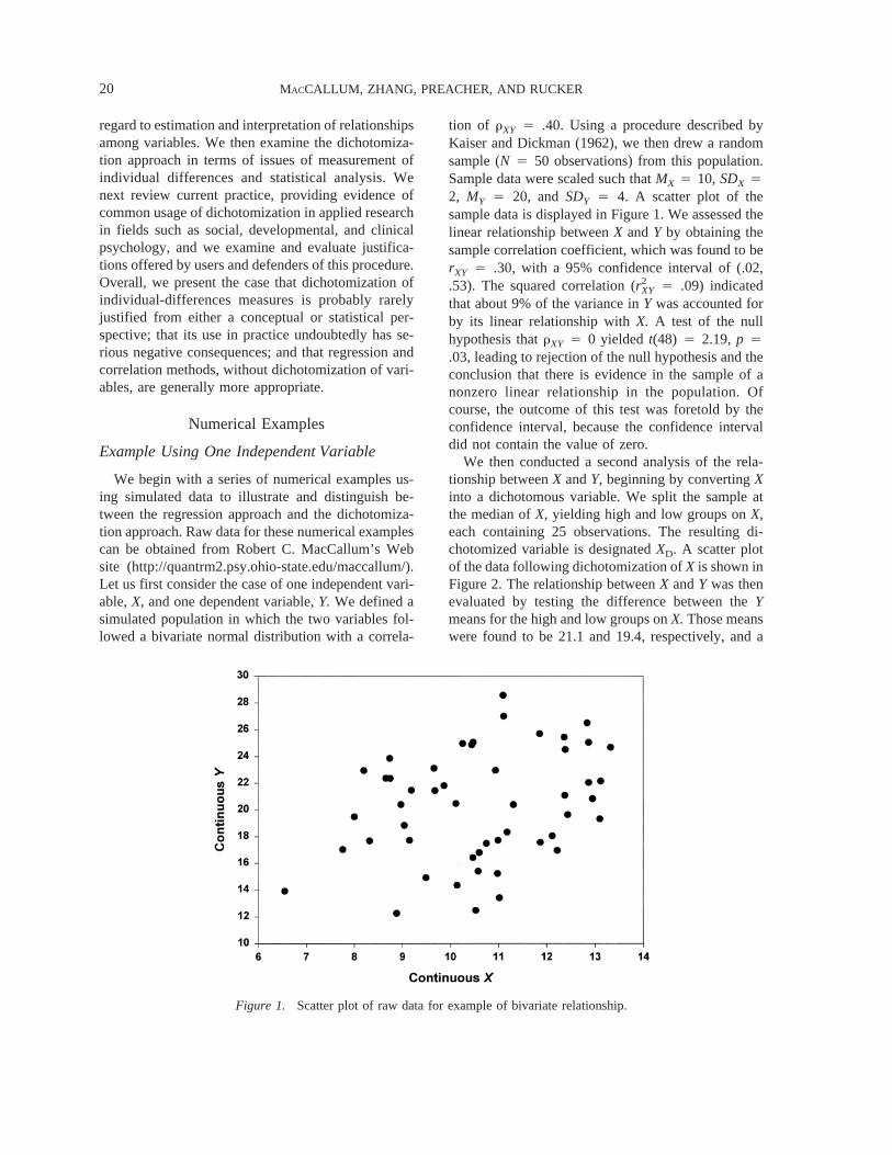
tion of rXY 4 .40. Using a procedure described byKaiser and Dickman (1962), we then drew a randomsample (N 4 50 observations) from this population.Sample data were scaled such thatMX 4 10, SDX 42, MY 4 20, andSDY 4 4. A scatter plot of thesample data is displayed in Figure 1. We assessed thelinear relationship betweenX andY by obtaining thesample correlation coefficient, which was found to berXY 4 .30, with a 95% confidence interval of (.02,.53). The squared correlation (r2

XY 4 .09) indicatedthat about 9% of the variance inY was accounted forby its linear relationship withX. A test of the nullhypothesis thatrXY 4 0 yieldedt(48) 4 2.19,p 4.03, leading to rejection of the null hypothesis and theconclusion that there is evidence in the sample of anonzero linear relationship in the population. Ofcourse, the outcome of this test was foretold by theconfidence interval, because the confidence intervaldid not contain the value of zero.

We then conducted a second analysis of the rela-tionship betweenX andY, beginning by convertingXinto a dichotomous variable. We split the sample atthe median ofX, yielding high and low groups onX,each containing 25 observations. The resulting di-chotomized variable is designatedXD. A scatter plotof the data following dichotomization ofX is shown inFigure 2. The relationship betweenX andY was thenevaluated by testing the difference between theYmeans for the high and low groups onX. Those meanswere found to be 21.1 and 19.4, respectively, and a

Figure 1. Scatter plot of raw data for example of bivariate relationship.

MACCALLUM, ZHANG, PREACHER, AND RUCKER20

test of the difference between them yieldedt(48) 41.47, p 4 .15, resulting in failure to reject the nullhypothesis of equal population means. From a corre-lational perspective, the correlation after dichotomi-zation wasrXDY 4 .21 (r2

XDY 4 .04), with a 95%confidence interval of (−.07, .46). Again, the confi-dence interval implies the result of the significancetest, this time indicating a nonsignificant relationshipbecause the interval did include the value of zero. Acomparison of the results of analysis of the associa-tion betweenX andYbefore and after dichotomizationof X shows a distinct loss of effect size and loss ofstatistical significance; these issues are addressed indetail later in this article.

The dichotomization procedure can be taken onestep further by splitting bothX andY, thereby yieldinga 2 × 2frequency table showing the association be-tween XD and YD. In the present example, this ap-proach yielded frequencies of 13 in the low–low andhigh–high cells and frequencies of 12 in the low–highand high–low cells. The corresponding test of asso-ciation x2

1(1, N 4 50) 4 0.08, p 4 .78, showed anonsignificant relationship between the dichotomizedvariables, which was also indicated by the small cor-relation between them,rXDYD

4 .06 with a 95% con-fidence interval of (−.22, .33). Note that the dichoto-mization of bothX and Y has further eroded thestrength of association between them.

Example Using Two Independent Variables

We next consider an example where there are twoindependent variables,X1 and X2. In practice suchdata would appropriately be treated by multiple re-gression analysis. However, a common approach in-stead is to convert bothX1 andX2 into dichotomousvariables and then to conduct ANOVA using a 2 × 2factorial design. We provide an illustration of bothmethods. Following procedures described by Kaiserand Dickman (1962), we constructed a sample (N 4100 observations) from a multivariate normal popu-lation such that the sample correlations among thethree variables would have the following pattern:rX1Y

4 .70, rX2Y4 .35, andrX1X2

4 .50. To examine therelationship ofY to X1 and X2, we first conductedmultiple regression analyses. Without loss of gener-ality, regression analyses were conducted on stan-dardized variables,ZY, Z1, andZ2. Using a linear re-gression model with no interaction term, we obtaineda squared multiple correlation of .49 with a 95% con-fidence interval of (.33, .61).1 This squared

1 Confidence intervals for squared multiple correlationsare useful but are not commonly provided by commercialsoftware for regression analysis. A free program offered byJames Steiger, available from his Web site (http://

Figure 2. Scatter plot for example of bivariate relationship after dichotomization ofX. (Notethat there is some overlapping of points in this figure.)

DICHOTOMIZATION OF QUANTITATIVE VARIABLES 21

multiple correlation was statistically significant,F(2,97)4 46.25,p < .01. The corresponding standardizedregression equation was

ZY 4 .70(Z1) + .00(Z2).

The coefficient forZ1 was statistically significant,b1

4 .70, t(1) 4 8.32,p < .01, whereas the coefficientfor Z2 obviously was not significant,b2 4 .00,t(1) 40.00,p 4 1.00, indicating a significant linear effect ofZ1 on ZY, but no significant effect ofZ2. Inclusion ofan interaction termZ3 4 Z1Z2 in the regression modelincreased the squared multiple correlation slightly to.50. The corresponding regression equation was

ZY 4 .72(Z1) − .01(Z2) − .07(Z3).

The standardized regression coefficient forZ1 wasstatistically significant,b1 4 .72, t(1) 4 8.38, p <.01, whereas the other two coefficients were not,b2

4 −.01, t(1) 4 −0.12,p 4 .96, andb3 4 −.07, t(1)4 −1.11, p 4 .27, indicating no significant lineareffect of Z2 and no significant interaction.

We then conducted a second analysis on the samedata, beginning by dichotomizingX1 andX2 by split-ting both at the median to createX1D andX2D. Resultsof a two-way ANOVA yielded a significant main ef-fect for X1D, F(1, 96)4 42.50,p < .01; a significantmain effect forX2D, F(1, 96)4 5.26,p 4 .02; and anonsignificant interaction,F(1, 96)4 0.19,p 4 .67.Total variance accounted for by these effects was .40.Of special note in these results is the presence of asignificant main effect ofX2D that was not present inthe regression analyses but arose only after both in-dependent variables were dichotomized. This phe-nomenon is discussed further later in this article. It isalso noteworthy that total variance accounted for wasreduced from .50 prior to dichotomization to .40 afterdichotomization.

Summary of Examples

From these few examples it should be clear thatthere exist potential problems when quantitative inde-pendent variables are dichotomized prior to analysisof their relationship to dependent variables. The ex-ample with one independent variable showed a loss ofeffect size and of statistical significance followingdichotomization ofX. The example with two indepen-

dent variables showed a significant main effect fol-lowing dichotomization that did not exist prior to di-chotomization. Although many other cases andexamples could be examined, these simple illustra-tions reveal potentially serious problems associatedwith dichotomization. If phenomena such as those justillustrated would be common in practice, then di-chotomization of variables probably should not bedone unless rigorously justified. In the following sec-tion we examine these phenomena closely, focusingon the impact of dichotomization on measurement andrepresentation of individual differences as well as onresults of statistical analyses.

Measurement and Statistical Issues AssociatedWith Dichotomization

Representing Individual Differences

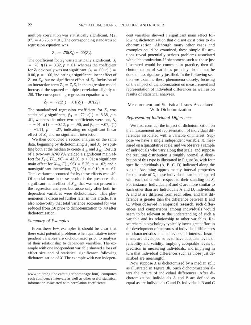
We first consider the impact of dichotomization onthe measurement and representation of individual dif-ferences associated with a variable of interest. Sup-pose we have a single independent variable,X, mea-sured on a quantitative scale, and we observe a sampleof individuals who vary along that scale, and supposethe resulting distribution is roughly normal. A distri-bution of this type is illustrated in Figure 3a, with fourspecific individuals (A, B, C, D) indicated along thex-axis. Assuming approximately interval propertiesfor the scale ofX, these individuals can be comparedwith each other with respect to their standing onX.For instance, Individuals B and C are more similar toeach other than are Individuals A and D. IndividualsA and B are different from each other, and that dif-ference is greater than the difference between B andC. When observed in empirical research, such differ-ences and comparisons among individuals wouldseem to be relevant to the understanding of such avariable and its relationship to other variables. Re-searchers in psychology typically invest great effort inthe development of measures of individual differenceson characteristics and behaviors of interest. Instru-ments are developed so as to have adequate levels ofreliability and validity, implying acceptable levels ofprecision in measuring individuals, and implying inturn that individual differences such as those just de-scribed are meaningful.

Now supposeX is dichotomized by a median splitas illustrated in Figure 3b. Such dichotomization al-ters the nature of individual differences. After di-chotomization, Individuals A and B are defined asequal as are Individuals C and D. Individuals B and C

www.interchg.ubc.ca/steiger/homepage.htm) computessuch confidence intervals as well as other useful statisticalinformation associated with correlation coefficients.


are different, even though their difference prior todichotomization was smaller than that between A andB, who are now considered equal. Following dichoto-mization, the difference between A and D is consid-ered to be the same as that between B and C. Themedian split alters the distribution ofX so that it hasthe form shown in Figure 3c. Clearly, most of theinformation about individual differences in the origi-nal distribution has been discarded, and the remaininginformation is quite different from the original. Suchan altering of the observed data must raise questions.What was the purpose of measuring individual differ-ences onX only to discard much of that informationby dichotomization? What are the consequences forthe psychometric properties of the measure ofX? Andwhat is the impact on results of subsequent analysesof the relationship ofX to other variables?

It seems that to justify such discarding of informa-tion, one would need to make one of two arguments.First, one might argue that the discarded informationis essentially error and that it is beneficial to eliminatesuch error by dichotomization. The implication of

such an argument would be that the true variable ofinterest is dichotomous and that dichotomization ofXproduces a more precise measure of that true di-chotomy. An alternative justification might involverecognition that the discarded information is not errorbut that there is some benefit to discarding it thatcompensates for the loss of information. Both of theseperspectives are discussed further later in this article.

Impact on Results of Statistical Analyses

Review of types of correlation coefficients and theirrelationships. Dichotomization of quantitative vari-ables affects results of statistical analyses involvingthose variables. To examine these effects, it is neces-sary to understand the meaning of and relationshipsamong several different types of correlation coeffi-cients. A correlation between two quantitatively mea-sured variables is conventionally computed as thecommon Pearson product–moment (PPM) correla-tion. A correlation between one quantitative and onedichotomous variable is a point-biserial correlation,and a correlation between two dichotomous variablesis a phi coefficient. The point-biserial and phi coeffi-cients are special cases of the PPM correlation. Thatis, if we apply the PPM formula to data involving onequantitative and one dichotomous variable, the resultwill be identical to that obtained using a formula fora point-biserial correlation. Similarly, if we apply thePPM formula to data involving two dichotomous vari-ables, the result will be identical to that obtained usinga formula for a phi coefficient. The point-biserial andphi coefficients are typically used in practice foranalyses of relationships involving variables that aretrue dichotomies. For example, one could use a point-biserial correlation to assess the relationship betweengender and extraversion, and one could use a phi co-efficient to measure the relationship between genderand smoking status (smoker vs. nonsmoker).

Some variables that are measured as dichotomousvariables are not true dichotomies. Consider, for ex-ample, performance on a single item on a multiplechoice test of mathematical skills. The measured vari-able is dichotomous (right vs. wrong), but the under-lying variable is continuous (level of mathematicalknowledge or ability). Special types of correlations,specifically biserial and tetrachoric correlations, areused to measure relationships involving such artificialdichotomies. Use of these correlations is based on theassumption that underlying a dichotomous measure isa normally distributed continuous variable. For thecase of one quantitative and one dichotomous vari-

Figure 3. Measurement of individual differences beforeand after dichotomization of a continuous variable.


able, a biserial correlation provides an estimate of therelationship between the quantitative variable and thecontinuous variable underlying the dichotomy. Forthe case of two dichotomous variables, the tetrachoriccorrelation estimates the relationship between the twocontinuous variables underlying the measured di-chotomies. Biserial correlations could be used to es-timate the relationship between a quantitative mea-sure, such as a measure of neuroticism as apersonality attribute, and the continuous variable thatunderlies a dichotomous test item, such as an item ona mathematical skills test. Tetrachoric correlations arecommonly used to estimate relationships betweencontinuous variables that underlie observed dichoto-mous variables, such as two test items.

Note that for the case of one quantitative and onedichotomous variable, one could calculate a point-biserial correlation, to measure the observed relation-ship, or a biserial correlation, to estimate the relation-ship involving the continuous variable underlying thedichotomous measure. The biserial correlation will belarger than the corresponding point-biserial correla-tion, because of the assumed gain in measurementprecision inherent in the former. In the population,the relationship between these two correlations isgiven by

rpb = rbS h

=pqD, (1)

wherep and q are the proportions of the populationabove and below the point of dichotomization, andhis the ordinate of the normal curve at that same point(Magnusson, 1966). Values ofh for any point of di-chotomization can be found in standard tables of nor-mal curve areas and ordinates (e.g., Cohen & Cohen,1983, p. 521).

For the case of two dichotomous variables, onecould compute either a phi coefficient to measure theobserved relationship or the tetrachoric correlation toestimate the relationship between the underlying di-chotomies. Again because of the assumed gain inmeasurement precision, the tetrachoric correlation ishigher than the corresponding phi coefficient. Al-though the general relationship between a phi coeffi-cient and a tetrachoric correlation is quite complex, itcan be defined for dichotomization at the mean asfollows:

rphi = 2@arcsin(rtetrachoric)#/p (2)

(Lord & Novick, 1968, p. 346). If the assumptions

inherent in the biserial and tetrachoric correlations arevalid, then the corresponding point-biserial correla-tion and phi coefficient can be seen to underestimatethe relationships of interest because of their failure toaccount for the artificial nature of the dichotomousmeasures. Given this background on correlation coef-ficients, we now turn to an examination of how di-chotomization of a quantitative variable impacts mea-sures of association between variables.

Analyses of effects of one independent variable.Various aspects of the impact of dichotomization onresults of statistical analysis have been examined anddiscussed in the methodological literature for manyyears. Here we review and examine in detail the mostimportant issues in this area, beginning with the sim-plest case of dichotomization of a single independentvariable. Basic issues associated with this case werediscussed by Cohen (1983). Suppose thatX and Yfollow a bivariate normal distribution in the popula-tion with a correlation ofrXY; variance inYaccountedfor by its linear relationship withX is thenr2

XY. If X isdichotomized at the mean to produceXD, then theresulting population correlation betweenXD andYcanbe designatedrXDY. (Note that for a normally distrib-uted variable, dichotomization at the mean and themedian are equivalent in the population.) To under-stand the impact of dichotomization on the relation-ship between the two variables, we must examine therelationship betweenrXY and rXDY. This relationshipcan be seen to correspond to the theoretical relation-ship between a biserial and point-biserial correlation.That is,rXDY corresponds to a point-biserial correla-tion, representing the association between a dichoto-mous variable and a quantitative variable, andrXY isequivalent to the corresponding biserial correlation,whereX is the continuous, normally distributed vari-able that underliesXD. The relationship between apoint-biserial and biserial correlation was given inEquation 1. Given this relationship, the effect of di-chotomization onrXY can then be represented as

rXDY = rXYS h

=pqD. (3)

The value ofh/√pq can be viewed as a constant, to bedesignatedd, representing the effect of dichotomiza-tion under normality. For example, ifX is dichoto-mized at the mean to produceXD, thenp 4 .50,q 4.50, h 4 .399, yieldingd 4 .798. The effect of di-chotomization on the correlation is then given byrXDY


4 (.798)rXY, with shared variance being reduced byr2

XDY 4 (.637)r2XY. To represent the effect of dichoto-

mization at points other than the mean, Figure 4shows the value ofd 4 h/√pq as a function ofp, theproportion of the population above the point of di-chotomization. It can be seen that as the point ofdichotomization moves further from the mean, theimpact on the correlation coefficient increases.Clearly there is substantial loss of effect size in thepopulation due to dichotomization at any point. Thisquantification of the loss is consistent with the sub-jective impression conveyed by Figures 1 and 2,where the linear relationship betweenX andYappearsto be weakened by dichotomization ofX.

The results in our numerical example reported ear-lier are consistent with these theoretical results. Oursample was drawn from a population whererXY4 .40and r2

XY 4 .16. Following dichotomization, thesepopulation values would becomerXDY 4 (.798)(.40)4 .32 andr2

XDY 4 (.637)(.16)4 .10. In our samplewe found that dichotomization reducedrXY 4 .30 torXDY 4 .21, and the corresponding squared correlationfrom .09 to .04. Thus, the proportional reduction ofeffect size in our sample was slightly larger thanwould have occurred in the population.

Of course, there would be sampling variability inthe degree of change fromrXY to rXDY. If we were togenerate a new sample (N 4 50) for our illustration,

we would obtain different values ofrXY andrXDY. Theimpact of dichotomization would vary from sample tosample. An interesting question is whether dichoto-mization could causerXY to increase, even under nor-mality, simply because of sampling error. This pointis relevant because researchers sometimes justify di-chotomization because of a finding that it yielded ahigher correlation. To examine this issue, we con-ducted a small-scale simulation study. We definedfive levels of population correlation,rXY 4 .10, .30,.50, .70, .90. We then generated repeated randomsamples from bivariate normal populations at eachlevel of rXY, using six different levels of sample size,N 4 50, 100, 150, 200, 250, 300. We generated10,000 such samples for each combination of levels ofsample size andrXY. In each sample we computedrXY,then dichotomizedX at the median and computedrXDY. For each combination ofrXYand sample size, wethen simply counted the number of times, out of10,000, thatrXDY > rXY, that is, the number of timeswhere dichotomization resulted in an increase in thecorrelation. Results are shown in Table 1. Of interestis the fact that when sample size andrXY were rela-tively small, it was not unusual to find that dichoto-mization resulted in an increase in the correlation be-tween the variables, simply due to sampling error.That is, even though, under bivariate normality, di-chotomization must cause the population correlation

Figure 4. Proportional effect of dichotomization ofX on correlation betweenX andY as afunction of point of dichotomization;p andq are the proportions of the population above andbelow the point of dichotomization, andh is the ordinate of the normal curve at the same point.


to decrease, application of this approach in smallsamples or whenrXY is relatively small can easilyresult in an increase in the sample correlation. Un-doubtedly in some cases such increases would cause acorrelation that was not statistically significant priorto dichotomization to become so after dichotomiza-tion. These results must raise a caution about potentialjustification of dichotomization in practice. A findingthat rXDY > rXY must not be taken as evidence thatdichotomization was appropriate or beneficial. In fact,under conditions typically found in psychological re-search, dichotomization will cause the population cor-relation to decrease; an observation of an increase inthe sample correlation in practice is very possiblyattributable to sampling error. Failure to understandthis phenomenon could easily cause inappropriatesubstantive interpretations.

The loss of effect size in the population followingdichotomization, and corresponding expected loss inthe sample, can affect the outcome of tests of statis-tical significance. In our earlier example, thet statisticfor testing the significance ofr dropped from 2.19prior to dichotomization to 1.47 after, and statisticalsignificance was lost. This loss of statistical signifi-cance can be attributed directly to loss of statisticalpower. Considering the power of the test of the nullhypothesis of zero correlation, we note that in ourexample, prior to dichotomization power was .84,based onrXY4 .40,N 4 50,a 4 .05, two-tailed test.After dichotomization ofX, power was reduced to .63,based onrXDY 4 (.798)(.40)4 .32. Such a loss ofpower would become more severe as the point ofdichotomization moves away from the mean, becausethe loss of effect size would be greater (see Figure 4).As noted by Cohen (1983), the loss of power causedby dichotomization can be viewed alternatively as aneffective loss of sample size. For instance, in our ex-

ample, prior to dichotomization, power of .63 couldhave been achieved with a sample size of only 32.Thus, the reduction in power from .84 to .63 due todichotomization was equivalent to reducing samplesize from 50 to 32, or discarding 36% of our sample.For a two-tailed test of the null hypothesis of zerocorrelation, usinga 4 .05, this effective loss ofsample size resulting from a median split will be con-sistently close to 36%. It will deviate from this levelwhen any of these aspects is altered, in particularbecoming greater when the point of dichotomizationdeviates from the mean.

Let us next consider the case where both the inde-pendent variableX and the dependent variableY aredichotomized, thereby converting a correlation ques-tion into analysis of a 2 × 2table of frequencies. Wecan examine the impact of double dichotomization byfocusing on the relationship betweenrXY and rXDYD

,the correlations before and after double dichotomiza-tion. The relationship between these values corre-sponds to the relationship between a phi coefficientand the corresponding tetrachoric correlation, assum-ing bivariate normality. The valuerXDYD

is a phi co-efficient, a correlation between two dichotomous vari-ables, and the valuerXY is the correspondingtetrachoric correlation, the correlation between nor-mally distributed variables,X andY, that underlie thetwo dichotomies,XD andYD. For dichotomization atthe mean, the relationship between the phi coefficientand the tetrachoric correlation was given in Equation2. In the present context, this relationship becomes

rXDYD4 2[arcsin(rXY)]/p (4)

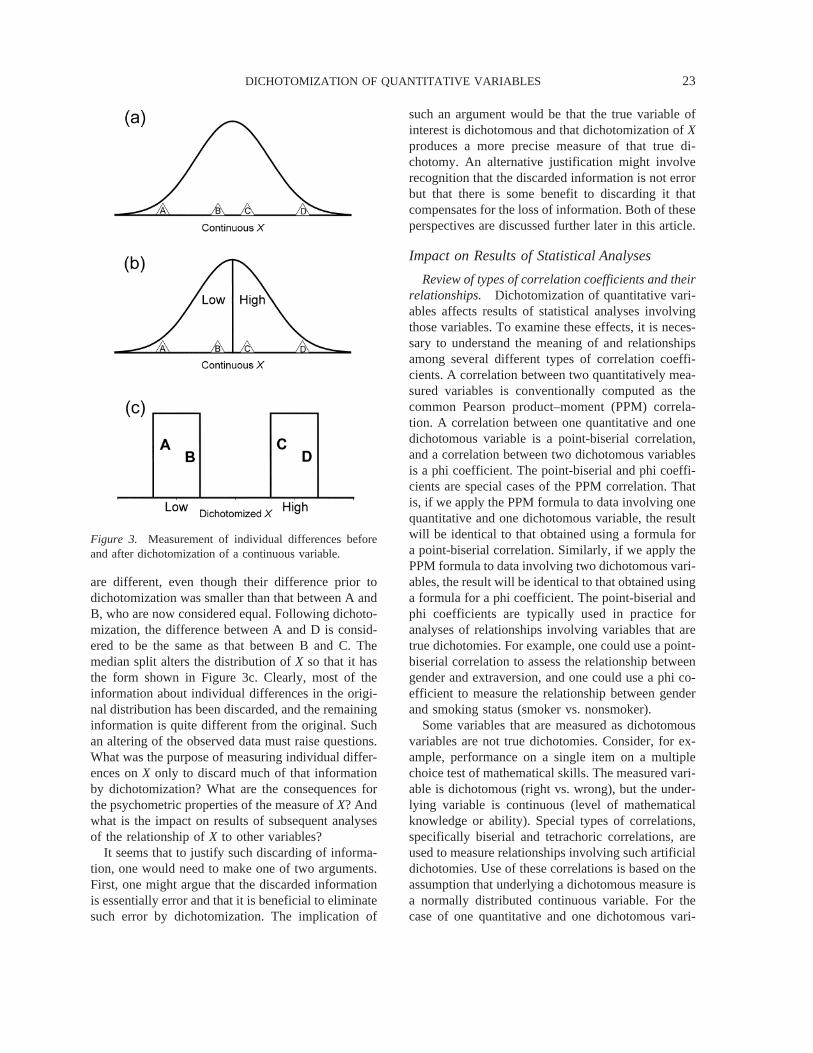
and thus represents the impact of double dichotomi-zation on the correlation of interest.2 This relationshipis shown in Figure 5, indicating the association be-tween population correlations obtained before di-chotomization (analogous to tetrachoric correlation,on horizontal axis) and after dichotomization (analo-gous to phi coefficient, on vertical axis). For instance,the value ofrXY 4 .40 in our example would bereduced torXDYD

4 .26. Our sample result showed aneven larger reduction, fromrXY 4 .30 torXDYD

4 .06.

2 For the case of dichotomization of both variables, Co-hen (1983) incorrectly assumed that the effect onrXYwouldbe the square of the effect of single dichotomization; forexample,rXDYD

4 (.798)2 rXY for dichotomization at themean. This same error occurs in Peters and Van Voorhis(1940) and was recognized by Vargha et al. (1996).

Table 1Frequency of Increase in Correlation Coefficient AfterDichotomization of Independent Variable for VariousLevels of Population Correlation (rXY) and Sample Size

rXY

N

50 100 150 200 250 300

.10 4,126 3,760 3,435 3,277 3,015 2,882

.30 2,430 1,620 1,109 776 612 434

.50 1,015 371 127 56 25 2

.70 173 12 3 1 0 0

.90 0 0 0 0 0 0

Note. Entries indicate the number of trials out of 10,000 in whichrXDY > rXY.


In general, loss of effect size is greater when bothvariables are dichotomized than when only one is di-chotomized. As the point of dichotomization movesaway from the mean, the relationship between the phicoefficient and tetrachoric correlation becomes muchmore complex (Kendall & Stuart, 1961; Pearson,1900), and the difference between the two coefficientsbecomes greater.

As in the case of dichotomization of onlyX, theloss of effect size under double dichotomization canbe represented as a loss of statistical power. In ourexample, power of the test of zero correlation wouldbe reduced from .84 prior to dichotomization to only.45 after dichotomization of bothX and Y. And asbefore, such loss of power could be represented as aneffective discarding of a portion of the originalsample. Loss of power, or effective loss of samplesize, becomes more severe if either or both of thevariables are dichotomized at points away from themean.

It is important to keep in mind that the effects ofdichotomization ofX, or of both X and Y, just de-scribed are based on the assumption of bivariate nor-mality of X andY. It may be tempting to conclude thatin empirical populations these effects would not hold.However, Cohen (1983) emphasized that these phe-nomena would be altered only marginally by nonnor-mality. It would require extreme skewness, hetero-scedasticity, or nonlinearity to substantially alter theseconsequences of dichotomization, conditions thatprobably are rather uncommon in social science data.When such conditions are present, that situation sim-

ply means that the formulas provided above for theinfluence of dichotomization on correlations mightnot hold closely. Such a complication does not pro-vide justification for dichotomization of variables.Rather, it would still be advisable not to dichotomize,but instead to retain information about individual dif-ferences and to consider resolving the extreme skew-ness, heteroscedasticity, or nonlinearity by use oftransformations of variables or nonlinear regression.

The issue of nonlinearity merits special attention.Suppose that the original relationship betweenX andY were nonlinear, such that a scatter plot such as thatin Figure 1 revealed a clear nonlinear association.Such a relationship could be represented easily usingnonlinear regression, and the investigator could obtainand present a clear picture of the association betweenthe variables. However, ifX, or both X and Y, weredichotomized, that nonlinear relationship would becompletely obscured. Presentation of results based onanalyses conducted after such dichotomization wouldbe misleading and invalid. Such errors can easily oc-cur accidentally if researchers dichotomize variableswithout examining the nature of the association be-tween the original variables.

Analyses of effects of two independent variables.We next examine statistical issues for the case of twoindependent variables,X1 andX2, and one dependentvariable,Y. The linear relationship ofX1 andX2 to Ycan be studied easily using regression methods. Stan-dard linear regression can be extended to investigateinteractive effects of the independent variables by in-troducing product terms (e.g.,X3 4 X1X2) into theregression model (Aiken & West, 1991). However, inpractice it is not uncommon for investigators to di-chotomize bothX1 andX2 prior to analysis and to useANOVA rather than regression. Over a period ofmore than 30 years, a number of methodological pa-pers have examined the impact of such an approachon statistical results and conclusions. Humphreys andcolleagues investigated several issues in this contextin a series of articles. Humphreys and Dachler (1969a,1969b) discussed an approach that they called apseudo-orthogonal designin which individuals areselected in high and low groups on bothX1 andX2 soas to produce a 2 × 2design with equal sample sizesin each cell. This approach does not involve dichoto-mization ofX1 andX2 after data have been collectedbut does involve treating individual-differences mea-sures as if they were categorical with only two levels.Such a design had been used by Jensen (1968) in astudy of the relationship of intelligence (X1) and so-

Figure 5. Relationship between phi and tetrachoric corre-lation for dichotomization ofX andY at their means.


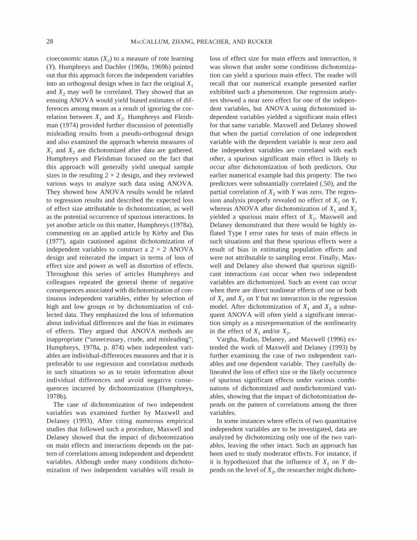
cioeconomic status (X2) to a measure of rote learning(Y). Humphreys and Dachler (1969a, 1969b) pointedout that this approach forces the independent variablesinto an orthogonal design when in fact the originalX1

andX2 may well be correlated. They showed that anensuing ANOVA would yield biased estimates of dif-ferences among means as a result of ignoring the cor-relation betweenX1 and X2. Humphreys and Fleish-man (1974) provided further discussion of potentiallymisleading results from a pseudo-orthogonal designand also examined the approach wherein measures ofX1 and X2 are dichotomized after data are gathered.Humphreys and Fleishman focused on the fact thatthis approach will generally yield unequal samplesizes in the resulting 2 × 2design, and they reviewedvarious ways to analyze such data using ANOVA.They showed how ANOVA results would be relatedto regression results and described the expected lossof effect size attributable to dichotomization, as wellas the potential occurrence of spurious interactions. Inyet another article on this matter, Humphreys (1978a),commenting on an applied article by Kirby and Das(1977), again cautioned against dichotomization ofindependent variables to construct a 2 × 2ANOVAdesign and reiterated the impact in terms of loss ofeffect size and power as well as distortion of effects.Throughout this series of articles Humphreys andcolleagues repeated the general theme of negativeconsequences associated with dichotomization of con-tinuous independent variables, either by selection ofhigh and low groups or by dichotomization of col-lected data. They emphasized the loss of informationabout individual differences and the bias in estimatesof effects. They argued that ANOVA methods areinappropriate (“unnecessary, crude, and misleading”;Humphreys, 1978a, p. 874) when independent vari-ables are individual-differences measures and that it ispreferable to use regression and correlation methodsin such situations so as to retain information aboutindividual differences and avoid negative conse-quences incurred by dichotomization (Humphreys,1978b).

The case of dichotomization of two independentvariables was examined further by Maxwell andDelaney (1993). After citing numerous empiricalstudies that followed such a procedure, Maxwell andDelaney showed that the impact of dichotomizationon main effects and interactions depends on the pat-tern of correlations among independent and dependentvariables. Although under many conditions dichoto-mization of two independent variables will result in

loss of effect size for main effects and interaction, itwas shown that under some conditions dichotomiza-tion can yield a spurious main effect. The reader willrecall that our numerical example presented earlierexhibited such a phenomenon. Our regression analy-ses showed a near zero effect for one of the indepen-dent variables, but ANOVA using dichotomized in-dependent variables yielded a significant main effectfor that same variable. Maxwell and Delaney showedthat when the partial correlation of one independentvariable with the dependent variable is near zero andthe independent variables are correlated with eachother, a spurious significant main effect is likely tooccur after dichotomization of both predictors. Ourearlier numerical example had this property: The twopredictors were substantially correlated (.50), and thepartial correlation ofX2 with Y was zero. The regres-sion analysis properly revealed no effect ofX2 on Y,whereas ANOVA after dichotomization ofX1 andX2

yielded a spurious main effect ofX2. Maxwell andDelaney demonstrated that there would be highly in-flated Type I error rates for tests of main effects insuch situations and that these spurious effects were aresult of bias in estimating population effects andwere not attributable to sampling error. Finally, Max-well and Delaney also showed that spurious signifi-cant interactions can occur when two independentvariables are dichotomized. Such an event can occurwhen there are direct nonlinear effects of one or bothof X1 andX2 on Y but no interaction in the regressionmodel. After dichotomization ofX1 and X2 a subse-quent ANOVA will often yield a significant interac-tion simply as a misrepresentation of the nonlinearityin the effect ofX1 and/orX2.

Vargha, Rudas, Delaney, and Maxwell (1996) ex-tended the work of Maxwell and Delaney (1993) byfurther examining the case of two independent vari-ables and one dependent variable. They carefully de-lineated the loss of effect size or the likely occurrenceof spurious significant effects under various combi-nations of dichotomized and nondichotomized vari-ables, showing that the impact of dichotomization de-pends on the pattern of correlations among the threevariables.

In some instances where effects of two quantitativeindependent variables are to be investigated, data areanalyzed by dichotomizing only one of the two vari-ables, leaving the other intact. Such an approach hasbeen used to study moderator effects. For instance, ifit is hypothesized that the influence ofX1 on Y de-pends on the level ofX2, the researcher might dichoto-


mizeX2 and then conduct separate regression analysesof Y on X1 for each level ofX2. Moderation is thenassessed by testing the difference between the tworesulting values ofrX1Y

, with a significant differencesupposedly indicating a moderator effect. It is impor-tant to note that most methodologists would adviseagainst such an approach for investigating moderatoreffects and would recommend instead the use of stan-dard regression methods that incorporate interactionsof quantitative variables (Aiken & West, 1991).

Bissonnette, Ickes, Bernstein, and Knowles (1990)conducted a simulation study to compare the dichoto-mization approach to the regression approach for ex-amining moderator effects. When no moderator effectwas present in the population, they found high Type Ierror rates under the dichotomization approach, indi-cating common occurrence of spurious interactions.Under the regression approach, Type I error rateswere nominal. When moderator effects were presentin the population, they found a higher rate of correctdetection of such effects using the regression ap-proach than the dichotomization approach. Given thedistortion of information incurred by dichotomizationalong with the inflated Type I error rates or loss ofpower, as well as the straightforward capacity of stan-dard regression to test for moderator effects, the useof the dichotomization method in this context seemsunwarranted and risky.

Finally, it should be noted that although our pre-sentation here has been limited to the cases of one ortwo independent variables, the issues and phenomenawe have examined are not limited to those cases. Thesame issues apply for designs with three or more in-dependent variables, although further complexitiesarise depending on the pattern of correlations amongthe variables and how many variables are dichoto-mized.

Aggregation and comparison of results across stud-ies. Regardless of the number of independent vari-ables, dichotomization raises issues regarding com-parison and aggregation of results across studies.Allison, Gorman, and Primavera (1993) cautionedthat dichotomization may introduce a lack of compa-rability of measures and results across studies. Forexample, groups defined as high or low after dichoto-mization may not be comparable between studies, es-pecially if the point of dichotomization is data depen-dent (e.g., the median). That is, the point ofdichotomization may vary considerably between stud-ies, thus making groups not comparable. Even whendichotomization is conducted using a predefined scale

point, resulting groups may differ considerably de-pending on the nature of the population from whichthe sample was drawn.

Hunter and Schmidt (1990) discussed problemscaused by dichotomization when results from differ-ent studies are to be aggregated using meta-analysis.They showed that dichotomization of one or moreindependent variables will tend to cause downwarddistortion of aggregated measures of effect sizes aswell as upward distortion of measures of variation ofeffect sizes across studies. They suggested methodsfor correcting these distortions in meta-analytic stud-ies. However, those methods do not resolve the prob-lem because they rely on their own assumptions andestimation methods. Such corrections are necessaryonly because of the persistent use of dichotomizationin applied research.

Summary of Impact of Dichotomization onMeasurement and Statistical Analyses

In this section we have reviewed literature on thevariety of negative consequences associated with di-chotomization. These include loss of informationabout individual differences, loss of effect size andpower, the occurrence of spurious significant maineffects or interactions, risks of overlooking nonlineareffects, and problems in comparing and aggregatingfindings across studies. To our knowledge, there havebeen no findings of positive consequences of dichoto-mization. Given this state of affairs, it would seemthat use of dichotomization in applied research wouldbe rather rare, but that is not at all the case. We nowexamine such usage in selected areas of applied re-search in psychology.

The Use of Dichotomization in Practice

Method

We selected six journals publishing research ar-ticles in clinical, social, personality, applied, and de-velopmental psychology. The specific journals se-lected wereJournal of Personality and SocialPsychology, Journal of Consulting and Clinical Psy-chology, Journal of Counseling Psychology, Develop-mental Psychology, Psychological Assessment,andJournal of Applied Psychology.These journals areknown for publishing research articles of high quality.The rationale behind selecting leading journals issimple. Leading journals are known for their high


standards, especially when statistical and method-ological considerations are present. If we were to findcommon use of dichotomization in high-quality jour-nals, this would suggest not only that uses of dichoto-mization must appear in other journals as well but alsothat leading researchers, as well as editors and review-ers, may be relatively unaware of the consequencesassociated with the use of dichotomization.

For each journal, we set out to examine all articlespublished from January 1998 through December2000. This time interval was selected so as to reflectcurrent practice. We limited our review to articlescontaining empirical studies, and we examined eachsuch article to determine if any measured variableshad been dichotomized prior to statistical analyses.An examination of articles published in 1998 in thesesix journals showed relatively frequent use of dichoto-mization in three of the journals—Journal of Person-ality and Social Psychology, Journal of Consultingand Clinical Psychology,andJournal of CounselingPsychology—but relatively rare usage in the otherthree—Developmental Psychology, Psychological As-sessment,and Journal of Applied Psychology.(Al-though Developmental Psychologycontained rela-tively few uses of dichotomization per se, it didcontain an abundance of examples wherein subjectswere divided into several groups based on chronolog-ical age.) Therefore, the full 3-year literature reviewwas conducted only on the former set of three jour-nals. In our review, we tabulated information aboutvarious forms of dichotomization, including mediansplits, mean splits, and other splits at selected scalepoints. We also noted other types of splits, such astertiary splits or selection of extreme groups, althoughsuch splits are not examined directly in this article.For each instance of dichotomization we noted thevariable that was split. In addition, we noted whetheror not a justification for the split was given and whatthat justification was.

Results

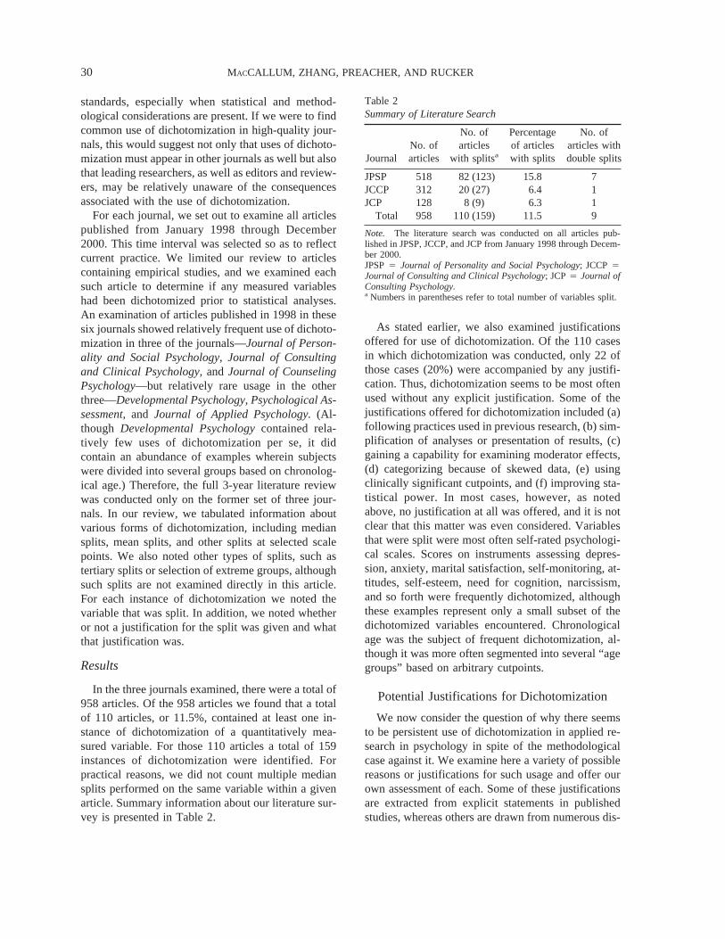
In the three journals examined, there were a total of958 articles. Of the 958 articles we found that a totalof 110 articles, or 11.5%, contained at least one in-stance of dichotomization of a quantitatively mea-sured variable. For those 110 articles a total of 159instances of dichotomization were identified. Forpractical reasons, we did not count multiple mediansplits performed on the same variable within a givenarticle. Summary information about our literature sur-vey is presented in Table 2.

As stated earlier, we also examined justificationsoffered for use of dichotomization. Of the 110 casesin which dichotomization was conducted, only 22 ofthose cases (20%) were accompanied by any justifi-cation. Thus, dichotomization seems to be most oftenused without any explicit justification. Some of thejustifications offered for dichotomization included (a)following practices used in previous research, (b) sim-plification of analyses or presentation of results, (c)gaining a capability for examining moderator effects,(d) categorizing because of skewed data, (e) usingclinically significant cutpoints, and (f) improving sta-tistical power. In most cases, however, as notedabove, no justification at all was offered, and it is notclear that this matter was even considered. Variablesthat were split were most often self-rated psychologi-cal scales. Scores on instruments assessing depres-sion, anxiety, marital satisfaction, self-monitoring, at-titudes, self-esteem, need for cognition, narcissism,and so forth were frequently dichotomized, althoughthese examples represent only a small subset of thedichotomized variables encountered. Chronologicalage was the subject of frequent dichotomization, al-though it was more often segmented into several “agegroups” based on arbitrary cutpoints.

Potential Justifications for Dichotomization

We now consider the question of why there seemsto be persistent use of dichotomization in applied re-search in psychology in spite of the methodologicalcase against it. We examine here a variety of possiblereasons or justifications for such usage and offer ourown assessment of each. Some of these justificationsare extracted from explicit statements in publishedstudies, whereas others are drawn from numerous dis-

Table 2Summary of Literature Search

JournalNo. ofarticles

No. ofarticles

with splitsa

Percentageof articleswith splits

No. ofarticles withdouble splits

JPSP 518 82 (123) 15.8 7JCCP 312 20 (27) 6.4 1JCP 128 8 (9) 6.3 1

Total 958 110 (159) 11.5 9

Note. The literature search was conducted on all articles pub-lished in JPSP, JCCP, and JCP from January 1998 through Decem-ber 2000.JPSP4 Journal of Personality and Social Psychology; JCCP4Journal of Consulting and Clinical Psychology; JCP4 Journal ofConsulting Psychology.a Numbers in parentheses refer to total number of variables split.


cussions with colleagues and applied researchers overa period of many years. Many researchers who usedichotomization are eager to defend the practice insuch discussions, and in the following sections we tryto provide a fair representation of such defenses.

Lack of Awareness of Costs

Some researchers who use dichotomization maysimply be unaware of its likely costs and negativeconsequences as delineated earlier in this article.When made aware of such costs, some of these indi-viduals may be eager to use more appropriate regres-sion methods and thereby avoid the costs and enhancethe measurement and statistical aspects of their stud-ies. We hope that the present article will have such animpact on researchers.

Perceiving Costs as Benefits

Some investigators acknowledge the costs but ar-gue that those very costs provide a justification fordichotomization. This argument is that because di-chotomization typically results in loss of measure-ment information as well as effect size and power, itmust yield a more conservative test of the relationshipbetween the variables of interest. Therefore, a findingof a statistically significant relationship following di-chotomization is more impressive than the same find-ing without dichotomization; the relationship must beespecially strong to still be found even when effectsize and power have been reduced. Essentially, thisargument reduces to the position that a more conser-vative statistical test is a benefit if it yields a signifi-cant result.

Let us consider this defense carefully. The argu-ment focuses on results of a test of statistical signifi-cance and also rests on the premise that dichotomiza-tion will make such tests and corresponding measuresof effect size more conservative. The focus on statis-tical significance is unfortunate, and the premise isfalse. First, regarding a focus on statistical signifi-cance, the American Psychological Association(APA) Task Force on Statistical Inference (Wilkinsonand the Task Force on Statistical Inference, 1999)urged researchers to pay much less attention to ac-cept–reject decisions and to focus more on measuresof effect size, stating that “reporting and interpretingeffect sizes . . . isessential to good research” (p. 599).In addition, thePublication Manual of the AmericanPsychological Association(5th ed.; APA, 2001) em-phasized that significance levels do not reflect the

magnitude of an effect or the strength of a relationshipand stated the following with respect to reporting re-sults: “For the reader to fully understand the impor-tance of . . . [a researcher’s] findings, it is almost al-ways necessary to include some index of effect size orstrength of relationship in . . . [the article’s] Resultssection” (p. 25). With regard to the present issue, thisperspective implies that it is misguided to focusmerely on whether or not a statistical test yields asignificant result after dichotomization. Rather, it isimportant to consider the size of the effect of interest.Our review of methodological issues presented earlieremphasized that dichotomization can play havoc withmeasures of effect size, generally reducing their mag-nitude in bivariate relationships and potentially reduc-ing or increasing them in analyses involving multipleindependent variables. Second, the belief that statis-tical tests will always be more conservative after di-chotomization is mistaken. Although this will tend tobe true in the case of dichotomization of a singleindependent variable, it is by no means always true.Our earlier results (see Table 1) showed that dichoto-mization may cause an increase in effect size simplydue to sampling error, thus producing a less conser-vative test. In addition, statistical tests may not bemore conservative when two or more independentvariables are dichotomized. In that case, as illustratedearlier, spurious significant main effects or interac-tions may arise depending on the pattern of intercor-relations between the variables. Thus, it is not at allthe case that dichotomization will always make a sta-tistical test or a measure of effect size more conser-vative.

Even if dichotomization did routinely yield moreconservative statistical tests and measures of effectsize, such a defense of its usage is highly suspect.Researchers typically design and conduct studies so asto enhance power and measures of effect size, as re-flected in efforts to use reliable measures, obtain largesamples, and use moderate alpha levels in hypothesistesting. If in fact more conservative tests were moredesirable and defensible, then perhaps researchersshould use less reliable measures, smaller samples,and small levels of alpha. One might then argue thatif significant effects were still found, those effectsmust be quite strong and robust. Of course, such anapproach to research would be counterproductive asare most uses of dichotomization. Our general view isthat this defense of dichotomization is not supportableon statistical grounds and is inconsistent with basicprinciples of research design and data analysis.


Lack of Awareness of Proper Methodsof Analysis

Over a period of many years, in discussions aboutdichotomization, we have encountered numerous re-searchers who simply have been unaware that re-gression/correlation methods are generally more ap-propriate for the analysis of relationships amongindividual-differences measures. This is especiallytrue of individuals whose primary training and expe-rience in the use of statistical methods is limited to orheavily emphasizes ANOVA. Of course, ANOVA isan important tool for data analysis in psychologicalresearch. However, difficulties and serious conse-quences arise when a problem that is best handled byregression/correlation methods is transformed into anANOVA problem by dichotomization of independentvariables. We are convinced that many researchers arenot sufficiently familiar with or aware of regression/correlation methods to use them in practice and there-fore often force data analysis problems into anANOVA framework. This seems especially true insituations where there are multiple independent vari-ables and the investigator is interested in interactions.We have repeatedly encountered the argument thatdichotomization is useful so as to allow for testing ofinteractions, under the (mistaken) belief that interac-tions cannot be investigated using regression meth-ods. In fact, it is straightforward to incorporate andtest interactions in regression models (Aiken & West,1991), and such an approach would avoid problemsdescribed earlier in this article regarding biased mea-sures of effect size and spurious significant effects.Furthermore, regression models can easily incorpo-rate higher way interactions as well as interactions ofa form other than linear × linear—for example, a lin-ear × quadratic interaction. Thus, we encourage re-searchers who use dichotomization out of lack of fa-miliarity with regression methods to invest the modestamount of time and effort necessary to be able toconduct straightforward regression and correlationalanalyses when independent variables are individual-differences measures.

A related issue, or underlying cause of this lack ofawareness of appropriate statistical methods, involvestraining in statistical methodology in graduate pro-grams in psychology. Results of surveys of such train-ing (Aiken, West, Millsap, & Taylor, 2000; Aiken,West, Sechrest, & Reno, 1990) indicate that educationin statistical methods is somewhat limited for manygraduate students in psychology and often focusesheavily on ANOVA methods. Although training in

regression methods is certainly available in many pro-grams, it receives less emphasis and is less often partof a standard program. Clearly, enhanced training inbasic methods of regression analysis could increaseawareness and usage of appropriate methods foranalysis of measures of individual differences andhelp to avoid some of the problems resulting fromoverreliance on ANOVA, such as the common usageof dichotomization.

Dichotomization Resulting inHigher Correlation

It is not rare for an investigator to dichotomize anindependent variable,X, and to find that the correla-tion betweenX and the dependent variable,Y, ishigher after dichotomization than before dichotomi-zation; that is,rXDY > rXY. Under such circumstances itmay be tempting for the investigator to believe thatsuch a finding justifies the use of dichotomization. Itdoes not. In our earlier discussion of the impact ofdichotomization on results of statistical analyses, wereviewed how population correlations would gener-ally be reduced. We also showed by means of a simu-lation study that this effect will not always hold insamples (see the results in Table 1). That is, simplybecause of sampling error, sample correlations mayincrease following dichotomization, especially whensample size is small or the sample correlation is small.Such an occurrence in practice may well be a chanceevent and does not provide a sound justification fordichotomization.

Dichotomization as Simplification

A common defense of dichotomization involves, inone form or another, an argument that analyses andresults are simplified. In terms of analyses, this argu-ment rests on the premise that an analysis of groupdifferences using ANOVA is somehow simpler thanan analysis of individual differences using regression/correlation methods. We suggest that proponents ofthis position may simply be more familiar and com-fortable with ANOVA methods and that the analysesand results themselves are not simpler. Both ap-proaches can be applied in routine fashion, and resultscan be presented in standard ways using statistics orgraphics. For instance, from our example of a bivari-ate relationship presented early in this article, corre-lational results showedrXY4 .30,r2

XY4 .09,t(48)42.19,p 4 .03. Figure 1 shows a scatter plot of the rawdata, which conveys an impression of strength of as-sociation. Results after dichotomization would be pre-


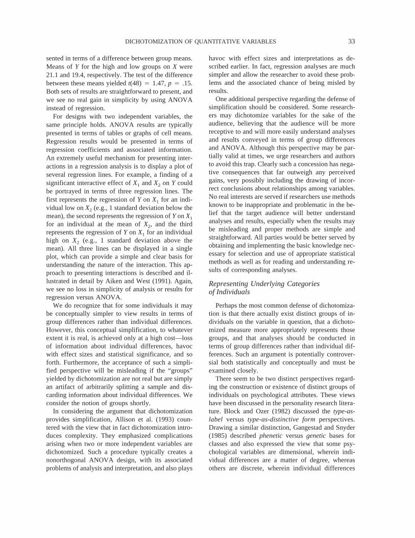
sented in terms of a difference between group means.Means ofY for the high and low groups onX were21.1 and 19.4, respectively. The test of the differencebetween these means yieldedt(48) 4 1.47,p 4 .15.Both sets of results are straightforward to present, andwe see no real gain in simplicity by using ANOVAinstead of regression.

For designs with two independent variables, thesame principle holds. ANOVA results are typicallypresented in terms of tables or graphs of cell means.Regression results would be presented in terms ofregression coefficients and associated information.An extremely useful mechanism for presenting inter-actions in a regression analysis is to display a plot ofseveral regression lines. For example, a finding of asignificant interactive effect ofX1 andX2 on Y couldbe portrayed in terms of three regression lines. Thefirst represents the regression ofY on X1 for an indi-vidual low onX2 (e.g., 1 standard deviation below themean), the second represents the regression ofYonX1

for an individual at the mean ofX2, and the thirdrepresents the regression ofY on X1 for an individualhigh on X2 (e.g., 1 standard deviation above themean). All three lines can be displayed in a singleplot, which can provide a simple and clear basis forunderstanding the nature of the interaction. This ap-proach to presenting interactions is described and il-lustrated in detail by Aiken and West (1991). Again,we see no loss in simplicity of analysis or results forregression versus ANOVA.

We do recognize that for some individuals it maybe conceptually simpler to view results in terms ofgroup differences rather than individual differences.However, this conceptual simplification, to whateverextent it is real, is achieved only at a high cost—lossof information about individual differences, havocwith effect sizes and statistical significance, and soforth. Furthermore, the acceptance of such a simpli-fied perspective will be misleading if the “groups”yielded by dichotomization are not real but are simplyan artifact of arbitrarily splitting a sample and dis-carding information about individual differences. Weconsider the notion of groups shortly.

In considering the argument that dichotomizationprovides simplification, Allison et al. (1993) coun-tered with the view that in fact dichotomization intro-duces complexity. They emphasized complicationsarising when two or more independent variables aredichotomized. Such a procedure typically creates anonorthogonal ANOVA design, with its associatedproblems of analysis and interpretation, and also plays

havoc with effect sizes and interpretations as de-scribed earlier. In fact, regression analyses are muchsimpler and allow the researcher to avoid these prob-lems and the associated chance of being misled byresults.

One additional perspective regarding the defense ofsimplification should be considered. Some research-ers may dichotomize variables for the sake of theaudience, believing that the audience will be morereceptive to and will more easily understand analysesand results conveyed in terms of group differencesand ANOVA. Although this perspective may be par-tially valid at times, we urge researchers and authorsto avoid this trap. Clearly such a concession has nega-tive consequences that far outweigh any perceivedgains, very possibly including the drawing of incor-rect conclusions about relationships among variables.No real interests are served if researchers use methodsknown to be inappropriate and problematic in the be-lief that the target audience will better understandanalyses and results, especially when the results maybe misleading and proper methods are simple andstraightforward. All parties would be better served byobtaining and implementing the basic knowledge nec-essary for selection and use of appropriate statisticalmethods as well as for reading and understanding re-sults of corresponding analyses.

Representing Underlying Categoriesof Individuals

Perhaps the most common defense of dichotomiza-tion is that there actually exist distinct groups of in-dividuals on the variable in question, that a dichoto-mized measure more appropriately represents thosegroups, and that analyses should be conducted interms of group differences rather than individual dif-ferences. Such an argument is potentially controver-sial both statistically and conceptually and must beexamined closely.

There seem to be two distinct perspectives regard-ing the construction or existence of distinct groups ofindividuals on psychological attributes. These viewshave been discussed in the personality research litera-ture. Block and Ozer (1982) discussed thetype-as-label versus type-as-distinctive formperspectives.Drawing a similar distinction, Gangestad and Snyder(1985) describedpheneticversusgenetic bases forclasses and also expressed the view that some psy-chological variables are dimensional, wherein indi-vidual differences are a matter of degree, whereasothers are discrete, wherein individual differences


represent discrete classes. The type-as-label or phe-netic view is that classes are merely constructed fromdata and have no underlying meaning. That is, they donot represent distinct categories of individuals but areessentially arbitrary groups defined by partitioning asample according to scores on variables of interest.The partitioning may be carried out by an arbitrarysplitting of one or more scales or may be the result ofsome more sophisticated approach such as clusteranalysis. Regardless, the resulting groups have nosubstantive meaning as distinct categories. The type-as-distinctive-form or genetic view is based on thenotion that there exists a discrete structure of indi-vidual differences underlying the observed variationon quantitative measures. The underlying categorieshave a genetic basis and a causal role with regard toobserved measures. Meehl (1992) referred to suchclasses astaxons, and stated that quantitative mea-sures may distinguish among taxons in the sense thatthose classes differ in kind as well as degree.

In the context of psychological research, it is clearthat, to use Gangestad and Snyder’s (1985) terms,phenetically defined groups are not as interesting orimportant as genetically defined groups. The formerdo not provide any insight about variables of interest,nor about relationships of those variables to others. Infact, basing analyses and interpretation on such arbi-trary groups is probably an oversimplification and po-tentially misleading. Genetically defined groups areclearly more interesting, but also somewhat contro-versial when their existence is inferred from indi-vidual-differences measures. It would seem difficultto make a case that groups defined by dichotomizationof measures of such attributes as self-esteem, anxiety,and need for cognition are genetically based and rep-resent a discrete structure of individual differences.This is not to say that such structures do not exist.Meehl (1992; Waller & Meehl, 1998) suggested thatthere is ample empirical evidence to support the ex-istence of taxons, especially in the areas of personalityand clinical assessment.

An interesting case study regarding the potentiallycontroversial nature of this issue began with an articleby Gangestad and Snyder (1985), who presented aconceptual argument along with research results at-tempting to make the case that the variable self-monitoring has a discrete underlying structure. As-suming the observed distribution of scores on a self-monitoring measure to represent distinct classes, andusing methods for identifying latent classes or taxons(see Waller & Meehl, 1998), Gangestad and Snyder

made a case for the existence of discrete high and lowgroups that were split at about a 60:40 ratio. Millerand Thayer (1989) attempted to refute this purportedclass structure for self-monitoring based on variouscorrelational analyses that, they argued, supported thesystematic structure of individual differences beyondthe differences represented by a simple high–low di-chotomy. In a subsequent article, Gangestad andSnyder (1991) argued that the results obtained byMiller and Thayer were not germane to the view thatthere existed an underlying class structure for self-monitoring.

Regardless of which party had the upper hand inthis exchange and regardless of whether or not thereexist two distinct categories of individuals with re-spect to self-monitoring, a critical point is that theexistence of such classes is subject to study and analy-sis and must not be assumed. As emphasized byMeehl (1992), the question of whether a particularphenomenon is most appropriately viewed as dimen-sional, taxonic, or some mix of these is an empiricalquestion. Such issues can be examined using methodsfor identifying distinct classes or distributions of in-dividuals, given measures for a sample of individualson one or more variables. Waller and Meehl (1998)used the generic termtaxometric methodsfor suchtechniques. Taxometric methods include a variety oftechniques such as cluster analysis (methods for iden-tifying clusters of individuals from multivariate data;Arabie, Hubert, & De Soete, 1996), mixture models(methods for identifying distinct distributions of indi-viduals that combine to form an observed overall dis-tribution; Arabie et al., 1996; Waller & Meehl, 1998),and latent class analysis (methods for identifyingtypes of individuals based on multivariate categoricaldata; McCutcheon, 1987). In the present contextwhere we are considering the possible existence ofdistinct types or groups of individuals on single mea-sured variables, relevant taxometric methods wouldprobably be limited to univariate mixture models andsome clustering methods that could be applied tosingle variables. Regardless, whenever the researcherwishes to investigate or argue for the existence ofdistinct taxons, types, or classes, he or she shouldsupport the argument with taxometric analyses, ratherthan assume its validity.

Given this background, let us consider the defenseof dichotomization as a technique for representingtypes of individuals. It should be immediately clearthat dichotomization is not a taxometric method but israther a simple method for grouping individuals into


arbitrarily defined classes. Even if discrete latentclasses actually exist in a given case, the groups re-sulting from dichotomization may bear little or noresemblance to those latent classes. Dichotomizationassumes that the number of taxons is two and does notallow for the possibility that there are more than two.Furthermore, dichotomization at the median assumesthat the base rate for each of those two taxons is 50%.Dichotomization at some other scale point is probablyno less arbitrary in terms of unjustifiable assumptionsabout the number of taxons and their base rates. Al-though Meehl (1992) argued for the existence of tax-ons in some cases, he clearly saw little value in di-chotomization, cautioning that categories concoctedby dichotomization of some measure are simply arbi-trary classes and are not of interest to psychologists.In short, even if a researcher believes that there existdistinct groups or types of individuals and an under-lying taxonic structure, dichotomization is not a use-ful technique. It is based on untenable assumptionsand defines arbitrary classes that are unlikely to havemuch empirical validity. Rather, in such situations, aresearcher should apply taxometric methods to assessthe presence of latent classes and classify individualsinto groups for subsequent analyses.

Dichotomization and Reliability

In questioning colleagues about their reasons foruse of dichotomization, we have often encountered adefense regarding reliability. The argument is that theraw measure ofX is viewed as not highly reliable interms of providing precise information about indi-vidual differences but that it can at least be trusted toindicate whether an individual is high or low on theattribute of interest. Based on this view, dichotomi-zation, typically at the median, would provide a “morereliable” measure. Cohen (1983) mentioned this pos-sible justification but claimed that dichotomizingwould in fact reduce reliability by introducing errorsof discreteness. He did not elaborate on the effect ofdichotomization on measurement reliability. We ex-amine this issue in detail here and show that, underprinciples of classical measurement theory, dichoto-mization of a continuous variable does not refine theoriginal measurement, but on the contrary, makes re-liability substantially worse.

In classical measurement theory, an observed vari-able score,X, is assumed to be the sum of the truescore,T, and random error,e:

X 4 T + e. (5)

Under classical assumptions, reliability,rXX, is then

defined as the ratio of true variance to total variance(Allen & Yen, 1979; Magnusson, 1966):

rXX =sT

2

sT2 + se

2 =sT

2

sX2 . (6)

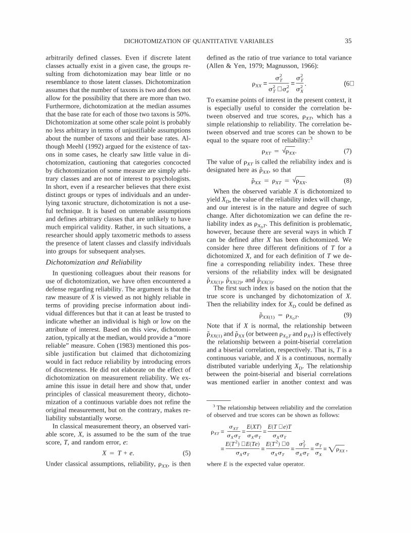
To examine points of interest in the present context, itis especially useful to consider the correlation be-tween observed and true scores,rXT, which has asimple relationship to reliability. The correlation be-tween observed and true scores can be shown to beequal to the square root of reliability:3

rXT 4 √rXX. (7)

The value ofrXT is called the reliability index and isdesignated here asrXX, so that

rXX 4 rXT 4 √rXX. (8)

When the observed variableX is dichotomized toyield XD, the value of the reliability index will change,and our interest is in the nature and degree of suchchange. After dichotomization we can define the re-liability index asrXDT. This definition is problematic,however, because there are several ways in whichTcan be defined afterX has been dichotomized. Weconsider here three different definitions ofT for adichotomizedX, and for each definition ofT we de-fine a corresponding reliability index. These threeversions of the reliability index will be designatedrXX(1), rXX(2), and rXX(3).

The first such index is based on the notion that thetrue score is unchanged by dichotomization ofX.Then the reliability index forXD could be defined as

rXX(1) 4 rXDT. (9)

Note that if X is normal, the relationship betweenrXX(1) andrXX (or betweenrXDT andrXT) is effectivelythe relationship between a point-biserial correlationand a biserial correlation, respectively. That is,T is acontinuous variable, andX is a continuous, normallydistributed variable underlyingXD. The relationshipbetween the point-biserial and biserial correlationswas mentioned earlier in another context and was

3 The relationship between reliability and the correlationof observed and true scores can be shown as follows:

rXT =sXT

sXsT=

E~XT!

sXsT=

E~T + e!T

sXsT

=E~T2! + E~Te!

sXsT=

E~T2! + 0

sXsT=

sT2

sXsT=

sT

sX= =rXX ,

whereE is the expected value operator.


specified in Equation 1. Adapting Equation 1 to thepresent context yields

rXX~1! = rXXS h

=pqD. (10)

For any specific dichotomizing point,rXX(1) is a con-stant proportion of the correspondingrXX, wherethe constant is given byd 4 h/√pq. For dichotomi-zation at any specified point, the effect on the reli-ability index is then given byrXX(1) 4 drXX. Fordichotomization at the mean,d 4 .798 (based onp 4.50, q 4 .50, h 4 .399). For dichotomization at 0.5standard deviations from the mean,d 4 .762 (basedon p 4 .691,q 4 .309,h 4 .352). For more extremedichotomization at 1.0 standard deviation,d 4 .662(based onp 4 .841, q 4 .159, h 4 .242). Thesevalues indicate the reduction in reliability due to di-chotomization, consideringT as unaltered. Figure 4,presented earlier in another context, can now beviewed as portraying the reduction in the reliabilityindex caused by dichotomization at any specifiedpoint on a normally distributedX.

We now consider a second way to conceptualizethe reliability of XD. Suppose we conceive of the di-chotomized measureXD as a measure of a dichoto-mized true variable,TD. That is, a perfectly reliableXD would indicate without error whether each indi-vidual is above or below the dichotomization splitpoint on the true score distribution. From this perspec-tive, the reliability index forXD could be defined as

rXX(2) 4 rXDTD. (11)

Note thatrXX(2) is a correlation between two dichoto-mous variables and is thus a phi coefficient. From thisperspective, ifX andT are both normal, then the origi-nal reliability index, orrXX, is effectively the corre-sponding tetrachoric correlation. The effect on reli-ability of dichotomization of bothX and T is thengiven by the relationship between a phi coefficientand a corresponding tetrachoric correlation. For thecase when both variables are dichotomized at themean, this relationship was specified in Equation 2 inanother context. Adapting Equation 2 to the presentcontext yields

rXX(2) 4 2[arcsin(rXX)]/p. (12)

Figure 5, presented earlier, can also be applied to thepresent context as showing the impact on reliabilitywhen bothX andT are dichotomized at the mean. Fordichotomization away from the mean, the relationshipbetween a phi coefficient and the corresponding tet-rachoric correlation becomes very complex with the

difference increasing as the split point deviates furtherfrom the mean, implying a greater impact on reliabil-ity in the present context.

A third definition of the reliability index after di-chotomization is based on defining the true score,according to classical measurement theory, as the ex-pected value of the observed measurement. If an in-dividual takes the same measurement repeatedly un-der appropriate conditions, or if he or she takesparallel tests, his or her true score would be equal tothe mean of an infinite number of such repeated mea-sures or parallel tests. This mean over an infinite num-ber of testings is represented formally using the ex-pected value operator,E, which indicates moregenerally the mean of a random variable over an in-finite number of samplings. In the present context, weexpress the true score for individuali as the expectedvalue of the observed score:

Ti 4 E(Xi). (13)

If the observed variableX is dichotomized, the corre-sponding true scoreT* becomes

Ti* = E~XDi!. (14)

For dichotomization at the split pointc, if the dichoto-mized observed variableX is coded as 1 if it is greaterthanc or as zero if not, the true score can be furtherexpressed as

Ti* = p~XDi = 1! = p~Xi . c ? Ti!. (15)

This true score for an observed variable after dichoto-mization is the conditional probability of the observedscore being greater thanc given the original undi-chotomized true score. The conditional probabilitydensity function ofXi givenTi is normal with meanTi

and variances2e. Therefore, the true score of indi-

vidual i after dichotomization is represented by thearea under the normal curve, with meanTi and vari-ances2

e, above the cutpointc. Formally, this is writtenusing the normal probability density function as

TDi* = *

c

`S 1

=2pse2DexpF− ~X − Ti!

2se2 GdX. (16)

Note thatT*D is a continuous variable. The correlation

between the dichotomized observed scoreXD and thenewly defined true scoreT*

D can be computed, and athird version of reliability index is defined as thiscorrelation:

rXX~3! = rXDTD* . (17)

It would be desirable to derive the functional relation-ship between this newly defined index of reliability,


rXX(3), and the original reliability index,rXX. How-ever, such an expression may not be tractable. Asimulation study to be presented shortly demonstratesthe relationship for some conditions.

In summary, we have presented three alternativedefinitions of the index of reliability when the mea-sureX is dichotomized. The first index,rXX(1), is thecorrelation between the dichotomized observed vari-able and the original true score; the second,rXX(2), isthe correlation between the dichotomized observedvariable and the dichotomized true score; and thethird, rXX(3), is the correlation between the dichoto-mized observed variable and the corresponding clas-sically defined true score, which is the expected valueof the dichotomized observed score. The relationshipsof rXX(1) andrXX(2) to the original reliability indexrXX

are specified in Equations 10 and 12, respectively.The relationship ofrXX(3) to rXX probably does nothave a tractable algebraic representation. These rela-tionships define the impact of dichotomization on re-liability under classical measurement theory.

To demonstrate and further examine this effect, weconducted a simple simulation study. Artificial datawere generated under the classical measurementmodel using four levels of the reliability coefficient:.60, .70, .80, and .90. Transformed to the reliabilityindex, these values correspond to .775, .837, .894, and.949, respectively. For each of these four conditions,a single large random sample (N 4 10,000) was gen-erated based on the classical measurement model(Equation 5). First, true scores and random errorswere generated independently. The true score was as-sumed unit normally distributed, and the random errorscore was normally distributed with a mean of zeroand a variance ofs2

e 4 1/rXX. True scores and ran-dom errors were then added to create observed scoresfor the 10,000 simulated individuals within each levelof reliability.

For each of these four large samples, the measureXwas then dichotomized at the median, and samplevalues of rXX(1), rXX(2), and rXX(3) were computed.Note that values ofrXX(1) and rXX(2) could be pre-dicted by Equations 10 and 12, respectively. Table 3shows squared values of these indices obtained afterdichotomization, along with predicted values forr2

XX(1) and r2XX(2). Squared values of the reliability in-

dex correspond to classically defined reliability. Notefirst that the values obtained from the simulated datawere very close to the predicted values. More gener-ally, results show clearly that dichotomization causedsubstantial decreases in reliability regardless of how

the true score is defined. The impact of dichotomiza-tion varied across levels of reliability and among thedifferent indexes examined but was always substan-tial.

This simulation study was extended to examine theeffect of dichotomization at points away from themean. As expected, as the point of dichotomizationdeviated further from the mean, the impact on reli-ability increased. Detailed results are not presentedhere but may be obtained from Robert C. MacCallum.

In summary, the foregoing detailed analysis showsthat dichotomization will result in moderate to sub-stantial decreases in measurement reliability under as-sumptions of classical test theory, regardless of howone defines a true score. As noted by Humphreys(1978a), this loss of reliable information due to cat-egorization will tend to attenuate correlations involv-ing dichotomized variables, contributing to the nega-tive statistical consequences described earlier in thisarticle. To argue that dichotomization increases reli-ability, one would have to define conditions that werevery different from those represented in classical mea-surement theory.

General Comments on Defensesof Dichotomization

We have considered a variety of defenses and jus-tifications that have been offered for the practice ofdichotomization of individual-differences measures.

Table 3Effect of Dichotomization at Mean on Reliability

Reliability beforedichotomization

Reliability after dichotomization

Observed Predicted

Reliability index (squared):r2XX(1)

.600 .375 .382

.700 .442 .446

.800 .514 .509

.900 .572 .573Reliability index (squared):r2

XX(2)

.600 .307 .318

.700 .386 .398

.800 .500 .497

.900 .642 .632Reliability index (squared):r2

XX(3)

.600 .399

.700 .487

.800 .596

.900 .716

Note. Definitions of alternative versions of the reliability index,rXX(1), rXX(2), andrXX(3), are provided in Equations 10, 12, and 17,respectively.


We believe that under close examination each of thesedefenses breaks down. Without valid justification, re-searchers who dichotomize individual-differencesmeasures are in a position of using a method that doesconsiderable harm to the analysis and understandingof their data, with no clear beneficial effects.

Legitimate Uses of Dichotomization?

Given that we have called into question a widerange of justifications that are often offered for di-chotomization, it is interesting to consider the ques-tion as to whether dichotomization is ever justified.Although we believe that there may be occasionalcases where it is justified, we emphasize that we be-lieve such cases to be very rare. Two such cases areconsidered here. One would be a situation in whichtaxometric analyses provided clear support for the ex-istence of two types or taxons within the observedsample, along with a clear scale point that differenti-ated the classes. Of importance, the existence of typesmust be supported by such analyses and must not beassumed or theorized. Even when such support is ob-tained, the classes in question almost certainly couldnot be identified by the commonly used median splitapproach because of the arbitrariness of the point ofdichotomization. Furthermore, the researcher mustrecognize that, even given clear evidence for the ex-istence of distinct groups, dichotomization wouldlikely result in the loss of reliable information aboutindividual differences within the groups, as well asmisclassification of some individuals. Claims of theexistence of types, and corresponding dichotomiza-tion of quantitative scales and analysis of group dif-ferences, simply must be supported by compellingresults from taxometric analyses.

A second possible setting in which dichotomizationmight be justified involves the occasional situationwhere the distribution of a count variable is extremelyhighly skewed, to the extent that there is a large num-ber of observations at the most extreme score on thedistribution. For example, suppose research partici-pants were asked how many cigarettes they smokedper day. A large number of people would give a re-sponse of “zero,” and the remainder of the samplewould show a distribution of nonzero values. Such adistribution indicates the presence of two groups ofpeople, smokers and nonsmokers. Corresponding di-chotomization of the measured variable would yield adichotomous indicator of smoking status, which maybe useful for subsequent analyses. However, an in-

vestigator following such a procedure must recognizethat such dichotomization involves loss of all infor-mation about variation among those individuals not atthe extreme scale point (e.g., variation in smokingfrequency among smokers). If such information is tobe retained and the variable is left intact, it is essentialto use specialized regression methods for analysis ofsuch variables; readers are referred to a discussion ofregression models for count variables in Long (1997).

Although there may be an occasional situation inwhich dichotomization is justified, we submit thatsuch circumstances are very rare in practice and donot represent common usage of dichotomization. Incommon usage, dichotomization is typically carriedout without apparent justification and without seriousawareness or regard for its consequences. Such ad hocprocedures are simply inappropriate and incur sub-stantial costs.

Summary and Conclusions

The methodological literature shows clearly andconclusively that dichotomization of quantitativemeasures has substantial negative consequences inmost circumstances in which it is used. These conse-quences include loss of information about individualdifferences; loss of effect size and power in the caseof bivariate relationships; loss of effect size andpower, or spurious statistical significance and overes-timation of effect size in the case of analyses with twoindependent variables; the potential to overlook non-linear relationships; and, as shown in this article, lossof measurement reliability. These consequences canbe easily avoided by application of standard methodsof regression and correlational analysis to original(undichotomized) measures.

Despite these circumstances, many researcherscontinue to apply dichotomization to measures of in-dividual differences. This practice may be due to fac-tors such as a lack of awareness of the consequencesor of appropriate methods of analysis, a belief in thepresence of types of individuals, or a belief that di-chotomization improves reliability. Such justifica-tions have been examined in the present article and,we believe, have been shown to be invalid.

Cases in which dichotomization is truly appropriateand beneficial are probably rare in psychological re-search and probably could be recognized only throughtaxometric analyses. Thus, we urge researchers whoare in the habit of dichotomizing individual-differences measures to carefully examine whethersuch a practice is justified. We also urge journal edi-


tors and reviewers to caution authors against the useof dichotomization in most situations, and we cautionconsumers of research to be skeptical regarding re-sults of studies wherein individual-differences mea-sures have been dichotomized. We hope that suchefforts will drastically reduce the practice of dichoto-mization and its negative impact on our scientific en-deavors.

References

Aiken, L. S., & West, S. G. (1991).Multiple regression:Testing and interpreting interactions.Newbury Park,CA: Sage.

Aiken, L. S., West, S. G., Millsap, R., & Taylor, A. (2000,October).Don’t shoot the messengers: First results fromthe survey of the quantitative curriculum of doctoral pro-grams in psychology.Paper presented at the meeting ofthe Society of Multivariate Experimental Psychology,Saratoga Springs, NY.

Aiken, L. S., West, S. G., Sechrest, L., & Reno, R. R.(1990). Graduate training in statistics, methodology, andmeasurement in psychology.American Psychologist, 45,721–734.

Allen, M. J., & Yen, W. M. (1979).Introduction to mea-surement theory.Monterey, CA: Sage.

Allison, D. B., Gorman, B. S., & Primavera, L. H. (1993).Some of the most common questions asked of statisticalconsultants: Our favorite responses and recommendedreadings.Genetic, Social, and General PsychologyMonographs, 119,155–185.

American Psychological Association. (2001).Publicationmanual of the American Psychological Association(5thed.). Washington, DC: Author.

Arabie, P., Hubert, L. J., & De Soete, G. (1996).Clusteringand classification.Singapore: World Scientific.

Bissonnette, V., Ickes, W., Bernstein, I., & Knowles, E.(1990). Personality moderating variables: A warningabout statistical artifact and a comparison of analytictechniques.Journal of Personality, 58,567–587.

Block, J., & Ozer, D. J. (1982). Two types of psychologists:Remarks on the Mendelsohn, Weiss, and Feimer contri-bution. Journal of Personality and Social Psychology,42,1171–1181.

Cohen, J. (1983). The cost of dichotomization.Applied Psy-chological Measurement, 7,249–253.

Cohen, J., & Cohen, P. (1983).Applied multiple regression/correlation analysis for the behavioral sciences.Hillsdale, NJ: Erlbaum.

Gangestad, S. W., & Snyder, M. (1985). “To carve nature at

its joints”: On the existence of discrete classes in person-ality. Psychological Review, 92,317–349.

Gangestad, S. W., & Snyder, M. (1991). Taxonomic analy-sis redux: Some statistical considerations for testing alatent class model.Journal of Personality and Social Psy-chology, 61,141–146.

Humphreys, L. G. (1978a). Doing research the hard way:Substituting analysis of variance for a problem in corre-lational analysis.Journal of Educational Psychology, 70,873–876.

Humphreys, L. G. (1978b). Research on individual differ-ences requires correlational analysis, not ANOVA.Intel-ligence, 2,1–5.

Humphreys, L. G., & Dachler, H. P. (1969a). Jensen’stheory of intelligence.Journal of Educational Psychol-ogy, 60,419–426.

Humphreys, L. G., & Dachler, H. P. (1969b). Jensen’stheory of intelligence: A rebuttal.Journal of EducationalPsychology, 60,432–433.

Humphreys, L. G., & Fleishman, A. (1974). Pseudo-orthogonal and other analysis of variance designs involv-ing individual-differences variables.Journal of Educa-tional Psychology, 66,464–472.

Hunter, J. E., & Schmidt, F. L. (1990). Dichotomization ofcontinuous variables: The implications for meta-analysis.Journal of Applied Psychology, 75,334–349.

Jensen, A. R. (1968). Patterns of mental ability and socio-economic status.Proceedings of the National Academy ofSciences, 60,1330–1337.

Kaiser, H. F., & Dickman, K. (1962). Sample and popula-tion score matrices and sample correlation matrices froman arbitrary population correlation matrix.Psy-chometrika, 27,179–182.

Kendall, M. G., & Stuart, A. (1961).The advanced theory ofstatistics: Vol. 2. Inference and relationship.New York:Hafner.

Kirby, J. R., & Das, J. P. (1977). Reading achievement, IQ,and simultaneous–successive processing.Journal of Ed-ucational Psychology, 69,564–570.

Long, J. S. (1997).Regression models for categorical andlimited dependent variables.Thousand Oaks, CA: Sage.

Lord, F. M., & Novick, M. R. (1968).Statistical theories ofmental test scores.Reading, MA: Addison-Wesley.

Magnusson, D. (1966).Test theory.Reading, MA: Addison-Wesley.

Maxwell, S. E., & Delaney, H. D. (1993). Bivariate median-splits and spurious statistical significance.PsychologicalBulletin, 113,181–190.

McCutcheon, A. C. (1987).Latent class analysis.BeverlyHills, CA: Sage.

Meehl, P. E. (1992). Factors and taxa, traits and types, dif-


ferences of degree and differences in kind.Journal ofPersonality, 60,117–174.

Miller, M. L., & Thayer, J. F. (1989). On the existence ofdiscrete classes in personality: Is self-monitoring the cor-rect joint to carve?Journal of Personality and SocialPsychology, 57,143–155.

Pearson, K. (1900). On the correlation of characters notquantitatively measurable.Royal Society PhilosophicalTransactions, Series A, 195,1–47.

Peters, C. C., & Van Voorhis, W. R. (1940).Statistical pro-cedures and their mathematical bases.New York: Mc-Graw-Hill.

Vargha, A., Rudas, T., Delaney, H. D., & Maxwell, S. E.(1996). Dichotomization, partial correlation, and condi-

tional independence.Journal of Educational and Behav-ioral Statistics, 21,264–282.

Waller, N. G., & Meehl, P. E. (1998).Multivariate taxomet-ric procedures: Distinguishing types from continua.Thousand Oaks, CA: Sage.

Wilkinson, L., and the Task Force on Statistical Inference.(1999). Statistical methods in psychology journals:Guidelines and explanations.American Psychologist, 54,594–604.

Received July 10, 2001Revision received October 25, 2001

Accepted October 25, 2001■


Documents

On the Practice of Dichotomization of Quantitative …€¦ · · 2010-05-28On the Practice of Dichotomization of Quantitative Variables ... The authors examine the practice of