Embed Size (px)
Citation preview

i
ON THE PREDICTABILITY OF TIME SERIES BY METRIC ENTROPY
A Thesis Submitted to the Graduate School of Engineering and Sciences of
İzmir Institute of Technology in Partial Fulfillment of the Requirements for the Degree of
MASTER OF SCIENCE
in Mechanical Engineering
by Hakkı Erhan SEVİL
July, 2006 İZMİR

ii
We approve the thesis of Hakkı Erhan SEVİL
Date of Signature ………………………… 12 July 2006 Asst. Prof. Dr. Serhan ÖZDEMİR Supervisor Department of Mechanical Engineering İzmir Institute of Technology ………………………… 12 July 2006 Prof. Dr. Ferit Acar SAVACI Department of Electrical and Electronics Engineering İzmir Institute of Technology ………………………… 12 July 2006 Asst.Prof. Dr. Şevket GÜMÜŞTEKİN Department of Electrical and Electronics Engineering İzmir Institute of Technology ………………………… 12 July 2006 Assoc. Prof. Dr. Barış ÖZERDEM Head of Department İzmir Institute of Technology
………………………… Assoc. Prof. Dr. Semahat ÖZDEMİR
Head of the Graduate School

iii
..and the future is certain..
...give use to work it out…*
* from the song “Road to Nowhere” by the American rock band “Talking Heads” (1985)

iv
ACKNOWLEDGMENTS
I would like to express my appreciation to my supervisor Asst. Prof. Dr. Serhan
ÖZDEMİR for his endless support and trust, encourage, ideas and comments throughout
the all steps of this study. I would like to acknowledge to my parents for their support
and patience. Also, I would like to thank to my colleagues in Mechatronics Laboratory
for their help throughout this study.

v
ABSTRACT
ON THE PREDICTABILITY OF TIME SERIES BY METRIC
ENTROPY
The computation of the metric entropy, a measure of the loss of information along
the attractor, from experimental time series is the main objective of this study. In this
study, replacing the current warning systems (simple threshold based, on/off circuits), a
new and promising prognosis system is tried to be achieved by the metric entropy, i.e.
Kolmogorov – Sinai entropy, from chaotic time series. Additional to metric entropy,
correlation dimension and time series statistical parameters were investigated.
Condition monitoring of ball bearings and drill bits was achieved in the light of
practical considerations of time series applications. Two different accelerated bearing
run-to-failure test rigs were constructed and the prediction tests were performed.
However, as a reason of shaft failure in both structures during the experiments, none of
them is completed. Finally, drill bit breakage experiments were carried out. In the
experiments, 10 small drill bits (1 mmφ ) were tested until they broke down, while
vibration data were consecutively taken in equal time intervals. After the analysis, a
consistent decrement in variation of metric entropy just before the breakage was
observed. As a result of the experiment results, metric entropy variation could be
proposed as an early warning system.

vi
ÖZET
ZAMAN SERİLERİNİN METRİK ENTROPİ YARDIMIYLA TAHMİN
EDİLEBİLİRLİĞİ
Bu çalışmanın birincil amacı, deneysel zaman serilerinde, çekici boyunca bilgi
kaybına eşit olan metric entropinin hesaplanmasıdır. Bu çalışmada, varolan basit eşik
değerine dayanan uyarı sistemleri yerine, kaotik zaman serilerinden metrik entropi ile,
diğer adıyla Kolmogorov-Sinai entropi ile, yeni ve umut verici bir hata teşhis sistemi
başarılmaya çalışılmıştır. Zaman serilerinin pratik kullanımı ışığında, rulman ve matkap
ucu durum izlemeleri gerçekleştirilmiştir. İki farklı hızlandırılmış rulman kırma test
düzeneği ve testleri yapılmıştır. Fakat, iki düzenekte de deney sırasında şaft kırılmaları
sonucu, testler tamamlanamamıştır. Son olarak, matkap ucu kırılma deneyleri
yapılmıştır. Deneylerde, 10 adet küçük matkap ucu (1 mmφ ) kırılana kadar test edilmiş
ve eşit aralıklı ardışık titreşim verileri alınmıştır. Analizler sonunda, metrik entropi
değişiminde, kırılmadan az önce, tutarlı bir düşme gözlenmiştir. Deneylerin sonucunda,
metrik entropi değişimi erken uyarı sistemi olarak önerilebilir.

vii
TABLE OF CONTENTS
LIST OF FIGURES............................................................................................................ ix
LIST OF TABLES .............................................................................................................xi
CHAPTER 1. INTRODUCTION ....................................................................................... 1
CHAPTER 2. TIME SERIES ANALYSIS......................................................................... 5
2.1. Nonlinear Dynamics................................................................................... 5
2.2. Characteristics of Chaotic Behavior........................................................... 6
2.3. Phase Space Representation....................................................................... 7
2.3.1. Attractor Geometry .............................................................................. 8
2.3.2. Reconstruction of Phase Space ............................................................ 8
2.3.2.1 Delay Reconstruction ...................................................................... 9
2.3.2.1.1. Autocorrelation ...................................................................... 10
2.3.2.1.2. Average Mutual Information.................................................. 11
2.3.2.2. Poincaré Sections ......................................................................... 12
2.4. Chaotic Invariants .................................................................................... 13
2.4.1. Correlation Dimension ....................................................................... 13
2.4.1.1. Correlation Sum ........................................................................... 13
2.4.2. Lyapunov Exponents.......................................................................... 16
2.4.3. Metric Entropy (Kolmogorov – Sinai Entropy)...................... ........... 18
2.4.3.1. Pesin Identity................................................................................ 20
CHAPTER 3. IMPLEMENTATION OF NONLINEAR
DYNAMICS IN TIME SERIES ................................................................ 21
3.1. Stationarity ............................................................................................... 21
3.2. Testing Nonlinearity................................................................................. 22
3.2.1. Method of Surrogate Data.................................................................. 22
3.2.1.1. Null Hypothesis (ARMA)……………..………….. .................... 22
3.2.2. Visual Inspection................................................................................ 26
3.3. Nonlinear Noise Reduction (State – Space Averaging) ........................... 27

viii
3.4. Tsonis Criteria.......................................................................................... 28
3.5. Finding Optimum Embedding Dimension ............................................... 29
3.5.1. False Nearest Neighbor ...................................................................... 29
3.5.2. Embedding Dimension – Correlation Dimension .............................. 31
3.6. Practical Considerations of Processing Time Series ................................ 31
3.6.1. Nyquist Sampling Rate Theorem ....................................................... 31
3.6.1.1. Aliasing ........................................................................................ 32
3.6.2. Time Series from Vibration Signal .................................................... 32
3.6.2.1. Accelerometer .............................................................................. 33
CHAPTER 4. METRIC ENTROPY APPLICATIONS
FOR CONDITION MONITORING.......................................................... 35
4.1. Experimental Setup .................................................................................. 35
4.1.1. Ball Bearing Failure Test Rig I .......................................................... 35
4.1.2. Ball Bearing Failure Test Rig II......................................................... 38
4.1.3. Drill Bit Breakage Test Rig................................................................ 39
4.2. Data Analysis ........................................................................................... 41
4.3. Experimental Results ............................................................................... 43
CHAPTER 5. CONCLUSION.......................................................................................... 47
REFERENCES.................................................................................................................. 48
APPENDICES
APPENDIX A. COMMON CHAOTIC SYSTEMS......................................................... 50
APPENDIX B. STATISTICAL PARAMETERS............................................................. 52
APPENDIX C. CULPERTUS .......................................................................................... 54

ix
LIST OF FIGURES
Figure Page
Figure 2.1. Phase Space Representation of Lorenz System ................................................ 7
Figure 2.2. Autocorrelation of Lorenz System.................................................................. 11
Figure 2.3. The average mutual information of Rössler System....................................... 12
Figure 2.4. Correlation sum demonstration....................................................................... 14
Figure 2.5. The correlation sum graph of Rössler system................................................. 15
Figure 2.6. Correlation Dimension graph of Lorenz system............................................. 16
Figure 2.7. Estimation of maximum Lyapunov Exponent.
In the graph (a), average distinction is calculated for various values.
(a) Average Distinction (b) Maximum Lyapunov Exponent .......................... 19
Figure 2.8. Metric Entropy of Henon Map which is calculated for embedding
dimensions 1 to 10....................................................................... ................... 19
Figure 3.1. Surrogate data of Henon map. (a) Original time series of Henon map
(b) One of the examples of the surrogates of Henon map
(c) Power spectrum of original series of Henon map
(d) Power spectrum of one of the examples of the surrogates of
Henon Map………………………………………………………………….. 26
Figure 3.2. Testing nonlinearity by using visual inspection
from embedding dimension-correlation dimension graph………………….. 27
Figure 3.3. Phase Portrait of ECG data (a) Before noise reduction
(b) After noise reduction…………………………………………………..... 28
Figure 3.4. False nearest neighbor graph of drill vibration data ....................................... 31
Figure 3.5. Embedding Dimension vs Correlation Dimension graph of Henon map ....... 32
Figure 4.1. Schematic of bearing test rig I ........................................................................ 36
Figure 4.2. The dents on the surface of the ball of bearing............................................... 37
Figure 4.3. (a) The experiment rig for ball bearing testing (b) Adjusted value of the
hydraulic jack shown in barometer ................................................................. 38
Figure 4.4. (a) Schematic of test rig II (b) A view of bearing test rig II ........................... 39
Figure 4.5. The schema of the test rig for drill bit breakage ............................................. 40
Figure 4.6. Schematic of lever force diagram ................................................................... 43
Figure 4.7. The broken drill bits........................................................................................ 43

x
Figure 4.8. Nonlinearity test of drill bit 3 with surrogate data.......................................... 44
Figure 4.9. Noise Reduction Process of drill bit 5 (a) Before Noise Reduction
(b) After Noise Reduction............................................................................... 44
Figure 4.10. (a)-(g) Metric Entropy graph of drill bit 7
(h) Metric entropy variation of drill bit 7........................................................ 45
Figure 4.11. (a)-(j) The metric entropy variations of all 10 drill bits 1 to 10 ................... 46
Figure A.1. Phase Portrait of Henon Map......................................................................... 50
Figure A.2. Phase Portrait of Lorenz Attractor ................................................................. 50
Figure A.3. Phase Portrait of Rössler Attractor ................................................................ 51
Figure C.1. Culpertus Open file ........................................................................................ 54
Figure C.2. Culpertus Save Image .................................................................................... 54
Figure C.3. Culpertus Autocorrelation.............................................................................. 55
Figure C.4. Culpertus Correlation Sum Parameters.......................................................... 55
Figure C.5. Culpertus Chaotic Invariants.......................................................................... 56

xi
LIST OF TABLES
Table Page
Table 2.1. Illustration of reconstructing of phase space.................................................... 10
Table 2.2. Characterization of the system via Lyapunov Exponents................................ 17
Table 4.1. Specification of experiment setup components ............................................... 41

1
CHAPTER 1
INTRODUCTION
Time series analysis comprises methods that attempt often either to understand
the underlying theory of the data points or to make forecasts of time series, which are
sequence of data points, measured typically at successive times spaced apart at uniform
time intervals. The last decade has brought dramatic changes in the way that researchers
analyze time series. Nonlinear time series analysis is becoming more and more reliable
tool for the study of complicated dynamics from measurements.
Most real-world systems are nonlinear and can be analyzed by nonlinear
techniques (Buzug 1994). Caputo et al. manage to analyze dynamic behavior of
fluidized bed systems from some selected time series data. The most impressive feature
of the nonlinear dynamics is chaos theory. Chaos is an aperiodic long-term behavior of
a bounded, deterministic system that has sensitive dependence on initial conditions,
where this feature is popularly known as “butterfly effect”.
Due to the fact that nearly all the observable phenomena in daily lives or in
scientific investigation are nonlinear, the importance of nonlinear dynamics is
increasing day by day. Chaos and nonlinear dynamics have provided new theoretical
and conceptual tools which allow comprehending the complex behaviours of systems.
Being a developing tool, through out the literature, various solutions are achieved by the
usage of these tools. Mechanical systems with backlash components were quantified by
the chaotic behaviour of the responses and correlation between the quantification
parameters and the parameters of the (non-linear) system is obtained (Tjahjowidodo et
al. 2005). Elshorbagy et al. (2002) analyzed time series in means of nonlinear
techniques for the estimation of missing stream flow data. After the chaotic behavior in
the daily flows of the river is investigated, the reconstructing of phase space of a time
series is utilized to identify the characteristics of the non linear dynamics.
In the literature on dynamical systems and chaos, the terms phase space and
state space are often used interchangeably. Phase space is a mathematical space which
is completely filled with trajectories, since each point can serve as an initial condition.

2
At any instant time the state of system can be completely specified by indicating a point
in state space.
Correlation dimension is a characteristic quantity for time series and has been
continuously gaining popularity by means of quantifying chaotic time series data.
Determination of the correlation dimension from experimental chaotic time series data
involves two steps. First, reconstruction of the phase space, then the computation of the
correlation dimension from the phase space vectors. The condition monitoring of
bearing systems with the effect of the gap clearance were characterized by the
application of embedding space and correlation dimension estimation (Craig et al.
2000). Furthermore, experimental results from a rolling element bearing from
experiment rig are successfully diagnosed by using correlation dimension. With
correlation dimension value, healthy and defected bearings were indicated. Also, defect
type classification was achieved (Logan 1995).
Chen et al. (1998) used the short term predictability feature of the chaotic
systems and phase space characterization to make one-hour to one-day predictions of
ozone levels. A reconstructed phase space model was applied to atmospheric
environment and used for the ozone levels prediction. The predictability of time series
can be indicated by metric entropy which is a measure of the rate of loss of
predictability. Metric entropy (as known as Kolmogorov – Sinai Entropy) obtains that
how far the future can be predicted with a given initial information. Drongelen et al.
(2003) demonstrated the feasibility of using analysis of the Metric Entropy of the time
series to anticipate seizures in pediatric patients with intractable epilepsy. Anticipation
times varied between 2 and 40 minutes.
Although most of the observable dynamical systems are nonlinear, before
applying nonlinear techniques, it is necessary to first ask, if the use of such advanced
techniques is justified by the data. Nonlinearity test with surrogate data is a process that
indicates the existence of the nonlinearity in the system (Schreiber 2001).
Another topic in nonlinear time series analysis is the effect of noise. Hegger et
al. (1999) proposed a simple nonlinear noise reduction for the analysis of observed
chaotic data. On the other hand, Elshorbagy et al. (2002) showed that the used of that
algotrithm for noise reduction might remove significant part of the original signal and
introduce nonexisting chaotic behaviour.
Condition monitoring of a machine can be thought as a decision support tool
which is able to indicate the development of probable failure in machinery component

3
or system, and that also predict failure occurrence. Even so, condition monitoring
allows avoidable actions which performed before a failure happened. The most
commonly used method for condition monitoring is vibration analysis. Although there
are different types of condition monitoring techniques currently in use for the diagnosis
and prediction of machinery faults, little attention has been paid to the detection of
chaotic behaviour in time series vibration signal. The field of condition monitoring is
always open to the introduction of new techniques for machine fault diagnosis.
Therefore comparisons can be drawn between combinations of several different
diagnosis techniques. Monitoring of a machining process is done by Govekar et al.
(2000) on the basis of sensor signal analysis. For signal analysis, methods of nonlinear
time series analysis are used. In recent years time series characterization is started to be
utilized as a condition monitoring and fault detection tool. Current fault detection
systems are simple threshold-based on-off circuits. The threshold values are determined
by experiments and set with an appropriate safety margin. These safety limits govern
the running of the machines, or human heart, and once set, they are not supposed to
change in time. In reality, these systems are not even needed. Since, no time or financial
losses might be spared when it is too late. For instance, on an assembly line, to predict
the failure of a failure-prone part within the work hours even before it has failed, and
replace it might prevent the whole line from squandering precious hours on idle.
Moreover on a vehicle, monitoring of a critical component real-time and on-line, and
maintaining a view of the part could save lives, and months-long litigations in court for
the manufacturers. Furthermore, a classification based method for condition monitoring
of robot joints using non-linear dynamics characteristics was proposed by Trendafilova
et al. (2000).
In the condition monitoring field, on-line tool condition monitoring has a great
significance in modern manufacturing processes. Sensing techniques, which have high
reliability, have been developed for providing a rapid response to an unexpected tool
breakage to prevent possible damages to the workpiece and machine component. Also,
several techniques on the detection of tool breakage for monitoring the drilling
processes have been developed over the past years (Xiaoli 1999 and Mori et al. 1999).
This study attempts to correlate the chaos invariants with the changing
conditions of a drilling process. Also, prediction of small drill bit breakage was
examined by using metric entropy. Briefly, the aim of this study is to introduce a
possible early damage detection method for mechanical systems.

4
This study presents experimental and a detailed analysis of mechanical drilling
system which shows chaotic behaviour. The computation of the invariants was carried
out by the TISEAN package (Hegger et al. 1999). In addition to that, various MatLAB
codes and time series analysing program Culpertus (Appendix C) were created.

5
CHAPTER 2
TIME SERIES ANALYSIS
Time series analysis comprises methods that attempt to understand the data
generating mechanism(s) of time series which are sequence of data points, measured
typically at successive times, spaced apart at uniform time intervals. There are two main
aims of time series analysis: (i) identifying the underlying theory of the phenomenon
represented by the data points, and (ii) making forecasts (predicting future values of the
time series variable). Both aims require the analyze of observed data point. Due to the
fact that the nonlinear dynamics of time series can produce chaotic time series, previous
data points are analized by nonlinear techniques.
2.1. Nonlinear Dynamics
The term dynamic refers to phenomena that produce time changing patterns,
where the characteristics of which at one time is interrelated with those at past times.
The dynamic of any situation refers to how the situation changes over the course of
time. A dynamical system is a physical setting together with rules for how the setting
changes or evolves from one moment of time to the next. Dynamical systems can be
either stochastic where the system evolve with respect to some random processes such
as the toss of coin, or deterministic where the future uniquely determined by the past
times.
Nonlinear systems represent systems whose behavior is not expressible as a sum
of the behaviors of its descriptors. In particular, the behavior of nonlinear systems is not
subject to the principle of superposition, as linear systems are. In nonlinear systems, a
small change in a parameter can lead to sudden and dramatic changes in both qualitative
and quantitative behavior of the system. As a result of this sensitivity, the behavior of
systems that exhibit chaos appears to be random, even though the system is
deterministic. The importance of nonlinear dynamics leans on the fact that nearly all the
observable phenomena in daily lives or in scientific investigation are nonlinear.

6
2.2. Characteristics of Chaotic Behavior
In mathematics and physics, although there is no universally accepted definition
of chaos, it is defined as “Stochastic behavior occurring in a deterministic system”. The
most important feature of chaos is the unpredictability of the future although it is a
deterministic system. Deterministic chaos refers to irregular or chaotic motion that is
generated by nonlinear systems evolving according to dynamical laws that uniquely
determine the state of the system at all times from a knowledge of the system's previous
history. It is important to point out that the chaotic behavior is due neither to external
sources of noise nor to an infinite number of degrees-of-freedom nor to quantum-
mechanical-like uncertainty. As a property of chaos, some sudden and dramatic changes
in systems may give rise to the complex behavior. Briefly, chaos is an aperiodic long-
term behavior of a deterministic system that has sensitive dependence on initial
conditions. The irregular behavior of chaotic system comes from the system’s
nonlinearity, although it has no random inputs or parameters as a deterministic system.
Also, as mentioned above, chaos is a long-term behavior, which means that in a chaotic
system, the trajectories do not settle down to a limit cycle, a fixed point, a periodic orbit
etc. A practical implication of chaos is that its presence makes it essentially impossible
to make any longterm predictions about the behavior of a dynamical system.
A chaotic dynamical system must satisfy the following requirements;
• The periodic orbits of the system must be dense,
• The system must be transitive,
• The system must be sensitive to initial conditions.
The density of periodic orbits in phase space is satisfied that for any point x in
phase space, any neighborhood of x contains at least a point from periodic orbits.
Furthermore, the transitivity means that no matter where the initial position on the
attractor, the dynamics’ trajectory will be arbitrarily close to every other point on the
attractor.
The most striking and the most known property of chaotic systems is the
sensitive dependence to initial conditions. Also it is popularly known as the "butterfly
effect". This property can be described simply as, exponential separation of the nearby

7
trajectories. even the difference of two initial positions is very small, that two points in a
chaotic system may move in extensively different trajectories, like flapping of a
butterfly's wings might create cause a tornado to occur over time. Only if the initial
conditions of two points are exactly the same, the system gives the same identical
results. In addition to that, for all chaotic systems, the trajectory of the system never
repeats.
2.3. Phase Space Representation
Phase space is a mathematical space spanned by the dependent variables of a
given dynamical system and in that space; all possible states of that system are
represented. In other words, phase space is a representor of a dynamical system where
each point on that phase space represents a particular state of the system at a particular
time (Figure 2.1).
Figure 2.1. Phase Space Representation of Lorenz System
Phase Space representation is versatile tool in time series analysis. Due to the
fact that, phase space determine all the states of a dynamical system, analysis of that
system can be achieved in both identifying the system and predicting the future states
via phase space representation. Because of phase space method is such a powerful
technique; so many algorithms depend on phase space representation exist. From time
series point of view, phase space representation is very useful, too. Although the actual
phase space (state space) is unknown in experimental one dimensional time series, as a

8
substitute, an embedded phase space can be reconstructed by delay reconstruction
technique. In that embedded phase space, the phase space analysis can be applied
because embedded phase space own the same geometric properties as the state space.
This fact arises from the fact that the attractor in reconstructed phase space is one-to-one
image of the attractor in state space.
2.3.1. Attractor Geometry
The strange behavior of chaotic systems has geometry of the set in phase space
formed by the trajectories of the system called the attractor which the trajectories in
phase space will have some final state on it, as the system evolves in time. Briefly, an
attractor is a set to which all neighboring trajectories converge. Moreover, the attractor
of a system determines the long-term behavior of that system. Basin of attraction for an
attractor is a set of initial positions which are giving rise to trajectories that approach to
a given attractor. Attractors are generally called as strange attractors, due to the fact
that they generally have a very complicated geometry, fractal (self similarity) structure,
in chaotic systems.
Strange attractors have some characteristic features, i.e. any orbit or trajectory
that starts on them stays on them for all time. Also, they have usually a noninteger
dimension which is less than the dimension of phase space, e.g. if the phase space is two
dimensional, the attractor will have a dimension less than two.
2.3.2. Reconstruction of Phase Space
Physical phase space is the most important problem in time series analysis due
to the fact that it is unknown. As a result, the computations are made in some alternative
space called embedded or reconstructed space. The embedded (reconstructed) space
enables to draw out a multidimensional description of state space dynamics from the
time series data of a single dynamical variable, and generalizes the quantitative
measures of chaotic behavior.
Behavior of trajectories has the same geometric and dynamical properties in the
properly constructed embedding space. Geometric and dynamical properties
characterize the actual trajectories in the full multidimensional state space for the

9
system. The behavior of the actual trajectories in the full state space is mimicked by the
trajectories in the embedding space.
Firstly, in 1980, Packard, Crutchfield, Farmer and Shaw suggested the theory of
generating a reconstruction space from a single time series to characterize nonlinear
dynamical systems, and the theory was completed by F.Takens. In 1981, he proved that
the time-delayed variables constitute an adequate embedding provided the measured
variable is smooth and couples to all the other variables.
2.3.2.1 Delay Reconstruction
The time-delayed embedding space is reconstructed state space chosen with the
minimum dimension for which the important dynamical and topological properties are
maintained. For most purpose this dimension need only be the next integer larger than
2DA, where DA is the attractor dimension. The reconstructed attractor is a one-to-one
image of the attractor in the original phase space, and this is the requirement of the
minimal sufficient embedding dimension “m”.
sn= ),,...,,( )1()2( vmnvmnvnn ssss −−−−− (2.1)
In this study, the time series analyses are processed as discrete time systems.
Therefore, replacing to the time lag τ for continuous systems, the sample lag v is used.
The relation between these two is; τ = v ∆ t, where ∆ t is the sampling interval of the
data.
Computationally, finding optimum value m takes few steps to the result. At the
beginning, although the optimal embedding dimension is unknown, embedding phase
space can be reconstructed for various values of m with using optimum time lag v, e.g.
for m=2,3,…7.
For reconstructing a embedding vector sn, first, the sample sn is taken into the
vector, and then v lagged sample sn+v, 2v lagged sample sn+2v, 3v lagged sample sn+3v are
added into the vector. The number of lagged samples which are added into the vector is
denoted by phase space dimension number m.
During the formulation of reconstruction of phase space vector, for m values, the
notation which varies between 0 to (m-1) is used. The reason of these is that every

10
vector sn has its own sample sn first (m=0). This notation of m values doesn’t effect the
dimension, because from 0 to (m-1) there are m pieces.
For the computational ease, the v next samples are added to the embedding
vector. The lag direction of the embedding vectors doesn’t make any difference. The
formula can be created with adding the v previous samples or v next samples.
sn= ),,...,,( )1()2( vmnvmnvnn ssss −+−++ (2.2)
Table 2.1. Illustration of reconstructing of phase space
Reconstructed Phase Space Dimension Phase Space Vector 1 2 … m-1 m
s1= s1 s1+v … s1+(m-2)v s1+(m-1)v s2= s2 s2+v … s2+(m-2)v s2+(m-1)v : : : ... : :
sn= sn sn+v … sn+(m-2)v sn+(m-1)v : : : … : :
sN-(m-1)v= sN-(m-1)v sN-(m-2)v … sN-v sN
The value of v needs computational process. Basically, this value represent the
inter relations between data samples. To find the optimum value of sample lag, either
autocorrelation which is linear correlation of a time series with its own past or mutual
information which is the probability about the value of sn+v when the value of sn is
known, is used.
2.3.2.1.1. Autocorrelation
The time evolution of a system can be analyzed by using the autocorrelation of a
signal. Autocorrelation measures how strongly on average each data point is correlated
with one time step away. It is the ratio of the autocovariance to the variance of the
data. Autocorrelation is a linear measure, each term of which measures the extent to
which sn versus sn+v is a straight line. The autocorrelation of a time series is;
2
1
)})({(1
σ
µµ∑=
+ −−=
N
n
vnn
v
ssN
c (2.3)

11
where µ is the mean value and the 2σ is the variance value of the time series.
In general the autocorrelation function falls from 1 at v=0 to 0 at large values of
v. In deterministic chaotic systems, the autocorrelation of the time series exponentially
decreases with increasing lag values, thus the value v at which it falls exponentially is
called the optimum correlation time. In implementation, firstly the vc values are
computed, with changing values of v in between 0 and∞ . The v value which first makes
vc ≈ 0 or the decay of vc exponentially is accepted as optimal lag (Figure 2.2). It is
clear by the equation that the aim is to find the samples that are highly correlated each
other with lag v. It should be noted that for a zero lag, autocorrelation equals to one.
2.3.2.1.2. Average Mutual Information
Mutual information is a tool to measures of independence between data samples.
Unlike the autocorrelation function which is based on linear statistics, the mutual
information takes into account also nonlinear correlations.
Figure 2.2. Autocorrelation of Lorenz System
Mutual information is simply gives probability about the value of sn+v, when the value
of sn is known. The computation of mutual information is;

12
∑∑ −=i
ii
ji
ijij ppvpvpvI )ln(2))(ln()()(,
(2.4)
First of all, from the time series data, a histogram is created including various
bins. The choice of the length of the bins (ε) is not important, as long as it is fine
enough. As in the equation, pi denotes the probability of sn being in the ith bin of the
histogram. Also pij denotes the probability of sn+v being in jth bin while sn is in the i
th bin
of the histogram. From the equation, the first minimum of the mutual information with
related lag, I(v), indicates the optimum sample lag where sn+v adds maximum
information to the knowledge which is gotten from sn (Figure 2.3).
Figure 2.3. The average mutual information of Rössler System
2.3.2.2. Poincaré Sections
Poincaré section is a method for indicating the structure of a flow in a phase
space more than two dimensions. Poincaré section is created by choosing a plane on the
trajectory and recording on that plane the points at which the trajectory intersects that
surface in a specified direction (same side of the plane). The intersection points give
information about the dynamical system’s behavior.
The choice of the poincaré section is not dependent on a rule. It need not be
perpendicular to the trajectory, but it must not be tangent to trajectory. However, for
better results, the placement of the plane must satisfied that it maximizes the number of

13
intersections with minimizes the time intervals between them. Depending to choice of
the section and the path in the reconstructed phase space, the intersection points will
vary. This method reduces the dimension of the attractor by one.
2.4. Chaotic Invariants
In experimental time series analyses, the chaotic invariants are used to determine
the system condition, to making estimations and even predictions. In this study,
invariants such as correlation dimension (a measure of the complexity that quantifies
the geometry and shape of strange attractors), Lyapunov exponents (a measure of
sensitivity of the process to initial conditions) and metric entropy (a measure of the loss
of information along the attractor) are taken to consideration for time series analyses.
Calculation of these invariants requires that the time series must be reconstructed into a
embedded phase space.
2.4.1. Correlation Dimension
Correlation dimension is a measure of the fractal dimension of the time series,
which measures the complexity that quantifies the geometry and shape of strange
attractor. The correlation sum is used to estimate the correlation dimension.
2.4.1.1. Correlation Sum
In chaos theory the correlation sum is the estimator of the correlation dimension.
The correlation sum for a collection of points sn in some vector space is the fraction of
all possible pairs of points which are closer than a given distance “epsilon” (ε ) in a
particular norm. The method of correlation sum consists of centering a hyper sphere on
a point in hyper-space or phase space, letting the radius of the hyper sphere grow until
all points are enclosed, and keeping track of the number of data points that are enclosed
by the hyper sphere (Figure 2.4).
Correlation sum C(ε ) is the number of points within all the circles of radius ε
(Figure 2.5). Similarly, correlation sum can be considered as the fact where the

14
probability of two different randomly chosen points will be closer than the distance ε .
It is expected that C(0)=0 for a chaotic system due to the fact that the points never
repeat in a non periodic system embedded without false nearest neighbor. The
correlation sum of a time series is computed by;
C(ε ) = )1(
2
−NN∑ ∑= +=
N
i
N
ij1 1
H(ε - ||si - sj||) (2.5)
where |||| • represent vector distance (euclid distance of two vectors) and H is
the heaviside step function.
Figure 2.4. Correlation sum demonstration
However, in a typical time series, the samples have correlation with each other
when they are close in time, besides of having correlation according to attractor
geometry. This kind of temporal correlations are excluded from the correlation sum by
updating the correlation sum formula;
C(ε ) = ))1()((
2
minmin −−− nNnN∑ ∑= +=
N
i
N
nij1 min
H(ε - ||si - sj||) (2.6)

15
Here, nmin values can be chosen generously as long as nmin<< N. The nmin value
is not large enough if it’s taken as the first zero of the autocorrelation or decay of
autocorrelation, so a bigger value than that must be chosen.
Figure 2.5. The correlation sum graph of Rössler system
The correlation sum just counts the pairs (si sj) whose distance is smaller than ε.
In the limit of an infinite amount of data (N→ ∞) and for small ε, it is expected that C to
scale like a power law;
C(ε) α εD (2.7)
According to this power law property a dimension value D, where based on the
behavior of a correlation sum, can be defined as;
εε
εε log
),(loglimlim)(
0
NCD
N ∞→→= (2.8)
This dimension is called correlation dimension and it’s a characteristic quantity
for time series. Correlation dimension simply shows that how C(ε) scales with ε. The
local slopes of the correlation sum graph constructs correlation dimension graph, and
the correlation dimension is equal to the average value of plateau region in the graph
(Figure 2.6).

16
Figure 2.6. Correlation Dimension graph of Lorenz system
Correlation dimension can also be used to determine whether a time series
derives from a random process or from a deterministic chaotic system. The variation of
correlation dimension according to embedding dimension is used to characterize the
time series in this mean. If the time series is a random process, D(m) increases
continuously. If the time series is a deterministic system, after some point D remains
constant. A plot of the correlation dimension as a function of the embedding dimension
indicates this property.
2.4.2. Lyapunov Exponents
The most important feature of chaos theory is the unpredictability of the long
term future although it is a deterministic time evolution. In chaos theory, “similar causes
have similar effects” belief is invalid except for short periods. Inherent instability of the
solutions causes this unpredictability, which is called sensitive dependence on initial
conditions.
Instability in time series leads two important concepts. Although they are
related, they are mentioned as different concepts. These are; loss of information quantity
as known as Kolmogorov – Sinai (metric) entropy, the other one is the simply
exponentially separation of the nearby trajectories a.k.a. Lyapunov exponent (λ ).
Lyapunov exponent, which shows the long term behavior of the time series, is a

17
fundamental property that characterizes the rate of separation of infinitesimally close
trajectories. Furthermore, the value of Lyapunov exponent represents the
characterization of the system, e.g. if λ is positive, the nearby trajectories diverge
exponential, which means existence of chaos.
Table 2.2. Characterization of the system via Lyapunov Exponents (Sprott 2003)
1λ 2λ 3λ 4λ Attractor Dimension
(-) (-) (-) (-) Equilibrium point 0
0 (-) (-) (-) Limit Cycle 1
0 0 (-) (-) 2-torus 2
0 0 0 (-) 3-torus 3
(+) 0 (-) (-) Strange (chaotic) >2
(+) (+) 0 (-) Strange (hyperchaotic) >3
Many different Lyapunov exponents can be defined for a dynamical system. It is
a result of multi dimension of phase space. However the most important Lyapunov
exponent is the one which is called maximal Lyapunov exponent.
Suppose that, in phase space, two points, which are close to each other with
distance =0ε ||1n
s -2ns ||, will diverge exponentially from each other after some step, and
the distance between them becomes; =∆nε || nns ∆+1- nns ∆+2
||. The relation with these two
distances can be obtained by; n
n e ∆∆ ≅ λεε 0 where λ is the Lyapunov exponent of that
trajectory. Moreover, for finding maximal Lyapunov exponent from reconstructed time
series data, firstly average distinction is calculated as:
∑ ∑= ∈
∆+∆+
−=∆
N
n U
nnnn
n nn
ssUN
nS1 )(0 0
0
0)(
1ln
1)(
sss (2.9)
where )(0nU s is the neighborhood of
0ns with diameter ε and0ns is the first
element of 0ns . Then, if S exhibits a linear increase with identical slope, this slope can
be taken as an estimate of maximal Lyapunov exponent (Figure 2.7).

18
In time series analysis, some modifications are applied to the data, e.g. rescaling,
shifting, phase space reconstruction. Lyapunov exponents aren’t affected by these
modifications.
2.4.3. Metric Entropy (Kolmogorov – Sinai Entropy)
The metric (Kolmogorov – Sinai) entropy is a kind of measure to characterize
chaotic motion of a system in an arbitrary-dimensional phase space. The metric entropy
is proportional with the rate of loss of information at the current state of a dynamical
system in the course of time. Meanwhile, metric entropy is a measure of the rate of lost
of predictability, which indicates that how far into the future can be predicted with a
given initial information. Metric entropy originate from information theory.
In time series analysis, information theory provides an important approach. If
the observation of a system is considered as a source of information with a stream of
numbers, then the information theory can supply quantitive answer to how much info
can be possessed about the future when entire past have been observed. The metric
entropy of a time series is;
),1(
),(loglimlim
0 εε
+=
→∞→ mC
mCK
εm
(2.10)
In metric entropy graph, estimated metric entropy is equal to the average value
of plateau region in the graph (Figure 2.8).
Metric entropy has units of inverse time (for continuous systems) or inverse
iteration (for discerete systems). The value of the metric entropy describes the type of
system, e.g. in random systems, the metric entropy is equal to infinity (1/0, zero step
ahead can be preticted), and in periodic systems, the metric entropy is equal to zero
(1/∞, all the information can be preticted). Metric entropy can not take negative values
and can be large for a chaotic system.

19
Figure 2.7. Estimation of maximal Lyapunov Exponent of Henon Map. In the graph (a),
average distinction is calculated for various ε values. (a) Average
Distinction (b) Maximum Lyapunov Exponent
Figure 2.8. Metric Entropy of Henon Map which is calculated for embedding
dimensions 1 to 10

20
2.4.3.1. Pesin’s Identity
Pesin's identity relates the sum of positive Lyapunov exponents to the entropy of
the system. Lyapunov exponents, which measure the exponential rate of divergence of
nearby trajectories, are related to metric entropy in a such way that the metric entropy is
equal to the sum of the positive Lyapunov exponents only when the natural measure is
continuous along the unstable directions, as it is usually the case for chaotic flows (Eq.
2.11). In 1977, Pesin proved that for certain classes of systems such as one dimensional
maps, the logisitic map, henon map and tent map, the metric entropy is equal to the sum
of positive Lyapunov exponents due to the fact that the system invariants are absolutely
continues all expanding dimensions.
∑>
=0, ii
iKλ
λ (2.11)

21
CHAPTER 3
IMPLEMENTATION OF NONLINEAR DYNAMICS
IN TIME SERIES
Beyond theoretical aspects, there are few concepts to be considered before the
analysis of the time series. Computation of invariants should be performed after some
tests and processes are applied to the experimental data. Also, some calculations of
invariants need parameters which are optimized to constant values. For a proper usage
of time series, preliminarily processes should be taken into consideration.
3.1. Stationarity
Stationarity is a property in which the mean, variance and autocorrelation
structure remains constant over time, in other words, the distribution of the variables
does not depend on time.
A first step in time series analysis requires to achieve stationarity in the data,
thus the stationarity test has to be made. Stationarity test can be done in few steps, these
steps are:
• Divide the series into equal length segments.
• Compute the mean value for each consecutive segment.
• Compare the segments’ means with the mean of the whole series. Compute the
standard error:
)1(
)(1
2
−
−∑=
NN
ssN
n where ∑=
=N
n
n Nss1
/ (3.1)
In time series analysis, stationarity is quite important to satisfy that the
invariants give the reliable results, while the series have no increasing or decreasing

22
trend, constant variance over time and constant autocorrelation structure. For instance,
wherever the segment is taken from, the dynamics should remain the same.
3.2. Testing Nonlinearity
The nonlinear analysis of time series use techniques for the underlying
nonlinearity which exists in time series. Indeed, the stochastic linear systems may have
very complicated structure. Even so, the application of nonlinear series methods has to
be guaranteed by determining the nonlinearity in the time series which will be analyzed.
Hence, before starting to analyze a time series by nonlinear techniques, it is needed to
apply nonlinearity test to the data. In this study, nonlinearity test is achieved by the
method of surrogate data.
3.2.1. Method of Surrogate Data
Surrogate data is way of describing time series, whether it derives from
nonlinear deterministic system or some linear process. For this purpose the null
hypothesis which consists of candidate linear process is created. The objective is to
reject the hypothesis. A typical null hypothesis would be that the data result from
Gaussian linear stochastic process.
3.2.1.1. Null Hypothesis (ARMA)
Autoregressive (AR) models include past observations of the dependent variable
in the forecast of future observations and moving average (MA) models include past
observations of the innovations noise process in the forecast of future observations of
the dependent variable of interest. Autoregressive-moving-average (ARMA) models are
time-series models that include both AR and MA components. Shortly, ARMA
indicates linear models of the autocorrelation in a time series. ARMA models can be
described by a series of equations.

23
∑ ∑= =
−− ++=AR MAM
i
M
j
jnjinin bsaas1 0
0 η (3.2)
Here η is independent Gaussian random numbers with zero mean and unit
variance and ARM and MAM are the orders of the ARMA process respectively, e.g. if
the order of autoregressive part is one 1=ARM , and the order of the moving average part
is two 2=MAM , then the ARMA process is expressed as ARMA (1, 2).
After creating surrogates, a statistics must be chosen to make comparison. This
statistics can be linear or nonlinear prediction error, two or more point correlation, any
kind of dimension etc. The task is to calculate this statistics for null hypothesis, data and
its surrogates, then to make comparison between the results. The deviation of results of
original data and its surrogates from result of null hypothesis, point out that the original
data doesn’t come from a linear process. Some of the statistics for making comparison
between null hypothesis and original data with its surrogates are shown below;
• Linear Prediction Error
Linear prediction and linear prediction error calculations are shown below;
iMn
M
i
in AR
AR
saas +−=
+ ∑+= ˆˆ1
01 (3.3)
where s shows the predicted value. The coefficient 0a can be omitted by
subtracting the mean from the data; µ−= nn ss . The coefficients ia are determined by
a best fit to whole time series.
∑∑−
=+−+
=
=1
11
N
Mn
qMnn
M
i
iiq
AR
AR
AR
ssac (3.4)
where iqc is the autocovariance matrix and q=1 to MAR
∑−
=+−+−=
1N
Mn
qMniMniq
AR
ARARssc (3.5)

24
The illustration of computing coefficient ia is shown below;
For 1=ARM ;
∑
∑
=
−
=+
=N
n
n
N
n
nn
s
ss
a
1
2
1
11
1 (3.6)
For 2=ARM ;
∑ ∑ ∑
∑ ∑∑∑
−−
−++−
−
−
=21
221
112
11
1
)( nnnn
nnnnnnn
ssss
sssssss
a (3.7)
the sums are
from 2=n to N
∑ ∑ ∑
∑ ∑∑∑
−−
+−−+−
−
−
=21
221
121111
2
)( nnnn
nnnnnnn
ssss
sssssss
a (3.8)
After creating the linear predictions of time series, the prediction error e is
computed for data sets. Root mean square (rms) prediction error is;
( )2ˆnn sse −= (3.9)
• High order correlations
Higher order correlation calculations can be used because they are fast in
computational time. Although the correlations are based on linear relations, higher-order
autocorrelation measures the time asymmetry which is a strong signature of
nonlinearity. One typical qth order quantity is;
∑+=
−−−
N
vn
q
vnn ssvN 1
)(1
(3.10)

25
The goal is making a comparison between null hypothesis and original data with
its surrogates, according to the results of the statistics chosen. For this purpose,
surrogates are created (Figure 3.1). Surrogate data sets should satisfy that they contain
correlated random numbers which have the same power spectrum as the original data.
The number of surrogates is computed by specified level of significance. For
significance of 95%, 19 surrogates must be created for testing (19 surrogates and one
original data make a total number of 20 time series. 1 in 20, 5%). For the purpose of
creating surrogate data, first of all, fast (discrete) Fourier transform of data is taken;
∑=
=N
n
Nkni
nk esN
s1
/21 π&&& (3.11)
where k is between zero and N. Then ks&&& values ate multiplied by random phases,
ki
kk essφ&&&=′~ where kφ are uniformly distributed in [0,2π). Finally, inverse FFT is
computed.
∑=
−′=′N
k
Nkni
kn esN
s1
/2~1 π (3.12)
After creating the surrogates, the statistics all K surrogate data sets are
computed. If the major statistic results of original and surrogate data sets deviate from
null hypothesis result, then the null hypothesis can be rejected. That majority is
determined by significance level (e.g. 19 of 20 data sets in 95% significance level).
Rejection of null hypothesis indicates nonlinearity of the time series. Otherwise, the
series are based on a linear process.

26
Figure 3.1. Surrogate data of Henon map. (a) Original time series of Henon map
(b) One of the examples of the surrogates of Henon map (c) Power spectrum
of original series of Henon map (d) Power spectrum of one of the examples
of the surrogates of Henon map
3.2.2. Visual Inspection
Alternatively, testing nonlinearity process can be performed by using visual
inspection from embedding dimension- correlation dimension graph. In chaotic time
series, correlation dimension of a time series levels off at certain point in embedding
dimension- correlation dimension graph. However, the surrogate data of that series
continue increasing in correlation dimension monotonically with increasing embedding
dimension.
The major purpose can be achieved by demonstrating embedding dimension-
correlation dimension plot of original data and its surrogate. The convergence of

27
original data and continues increment of its surrogate are sufficient to indicate that the
original data might not come from a linear stochastic process (Figure 3.2).
Figure 3.2. Testing nonlinearity by using visual inspection from embedding dimension-
correlation dimension graph.
3.3. Nonlinear Noise Reduction (State – Space Averaging)
A time series with noise can be described in two components; one contains the
signal, and the other one contains random fluctuations. The classical way to identify
these two components is applying time series to power spectrum to obtaining the
distinction and then using a filter for separation (e.g. Wiener filter). However, this
approach fails for deterministic chaotic time series. The reason of failure comes from
property of that kind of system. Such systems produce a broad band spectrum in which
power spectrum of the signal resembles the power spectrum of random noise.
Alternatively, a better approach, which is called nonlinear noise reduction (a.k.a.
state space averaging), can be used (Figure 3.3). Nonlinear noise reduction is process
which noisy measurements are replaced by better values. The process simply follows
few steps shown below;

28
• Reconstructing the embedding phase space,
• Finding the vectors sn which are in the ε neighborhood of 0ns , ε<− nn ss
0,
• Taking average of middle values (at [m/2]th column) of these vector,
• Replacing the original values with the new, averaged values )(s);
∑∈
−− =)(
)2/()2/(
00)(
1
nn U
mn
n
mn sU
ssss
) (3.13)
Figure 3.3. Phase Portrait of ECG data (a) Before noise reduction (b) After noise
reduction
In this algorithm, embedding dimension m should be taken a value that is higher
than m value needed by embedding theorems. Also, the neighborhood value ε should
be taken a value that is large enough to cover the noise size. However, ε value should
also be smaller than a typical curvature radius which exists in the time series. In this
approach, for the first and the last m/2 values of the time series, there is no correction
available. This algorithm allows applying multiply iterations with decreasing ε values
until no further change can be observed.
3.4. Tsonis Criteria
In time series analysis, the representation of the attractor is bounded with the
number of data. In order to make a confidential analysis of time series, complete
representation of the attractor and its geometric behavior should be satisfied. For a finite

29
data set, as the attractor dimension gets bigger, more data points are required to
determine its dimension. At this point, the term of required number of data points is
counted to the consideration. In the literature, controversial approximations exist.
However, the compromise suggestion about the required data points came from Tsonis
(1992). From his definition, the minimum sufficient data points for time series analysis
is obtained by;
ADN 4.02min 10 +α (3.14)
where DA is the attractor dimension. Additionally, from this equation, the
highest embedding dimension can be obtained from given N data point;
[ ]2)log(5.2 −NDA α (3.15)
Even though there is no guarantee for sufficiency of calculation the data points
from this equation, plausible estimations of necessary data can be achieved.
3.5. Finding Optimum Embedding Dimension
Finding optimum embedding is a significant process while it determines the
optimum reconstructed dimension which can be satisfactory for complete representation
of actual phase space. Due to the fact that deficient embedding dimension has not the
same geometric properties as the attractor in actual phase, the analyses, the computation
of the invariants and the conclusion results would be incorrect. Although, in this study,
constant embedding dimension value is not used for some invariants’ computation, such
as correlation dimension, calculation of all Lyapunov exponents of the system requires a
constant optimum embedding dimension.
3.5.1. False Nearest Neighbor
Suppose that, for a given time series, required minimal embedding dimension is
m0. This means that the time series should be reconstructed at least in m0, on the
condition that the reconstructed attractor is a one-to-one image of the attractor in the

30
original phase space. If time series is reconstructed to an smaller embedding dimension
than minimal embedding dimension, then the state space trajectories projection of the
points might appear as near neighborhoods of other points which they are not neighbor
in actual. These points are called false nearest neighbors.
To pass over this problem, it would be useful to increase the embedding
dimension step by step beginning from small values while controlling the false nearest
neighbors in each embedding. As the embedding dimension increases, the false nearest
neighbors to a particular point in the embedding space should decrease until the
embedding dimension is sufficiently large to cover the geometry of the attractor in
phase space. This algorithm is called the false nearest neighbor method which is a
method to determine the minimal sufficient embedding dimension introduced by Kennel
et al. in 1992 (Figure 3.4). The idea of this algorithm is the following:
• Find the nearest neighbor of each point in m-dimensional space,
• Calculate the distance,
• Iterate both points, calculate the distance and compute the ratio:
ji
ji
iRss
ss
+
+=
++ 11 (3.16)
The criterion for selection of the required minimum embedding dimension is
that the ratio of different embeddings converges at some point. The designation of the
false nearest neighbors is essential for the calculation of invariants, like the correlation
dimension, especially the Lyapunov exponent.

31
Figure 3.4. False nearest neighbor graph of drill vibration data
3.5.2. Embedding Dimension – Correlation Dimension
Another method for obtaining optimum embedding dimension is the visual
inspection from embedding dimension – correlation dimension graph. It is a fact that in
chaotic time series, correlation dimension for increasing embedding dimension become
constant after a saturation dimension level. In this way, optimum embedding dimension
can be found as computing correlation dimension for various embedding dimensions
and plot the results. In that plot, the level of embedding dimension where the correlation
dimension converges is accepted as the optimum embedding dimension (Figure 3.5).
3.6. Practical Considerations of Processing Time Series
In time series processing, an important concept, sampling rate, must be
considered to fulfill the desired data acquisition.
3.6.1. Nyquist Sampling Rate Theorem
Sampling is a process which consists of converting a continuous time signal into
a discrete time sequences. Discrete samples are a complete representation of the signal,
hence sampling rate, which is the interval of it discrete moments of time, is very
significant, because it would obtain how much detail the samples have about the signal.

32
According to the Nyquist Sampling Theorem, for the purpose of having no loss
information about the signal, the sampling rate should be greater than or equal to twice
the highest frequency present in the signal. When a signal is not sampled at a high
enough rate, aliasing occurs.
3.6.1.1. Aliasing
In sampling, the sampling rate should be at least twice value of the highest
frequency which exists in the signal. If the sampling rate is not high enough to sample
the signal correctly then a phenomenon called aliasing occurs. Mainly the term aliasing
refers to incorrect representation of the actual signal by the distortion which has a base
from lack of sampling rate. Moreover, aliasing indicates that the components of the
signal at high frequencies are replaced with components at lower frequencies by
mistaken.
Figure 3.5. Embedding Dimension vs Correlation Dimension graph of Henon map
3.6.2. Time Series from Vibration Signal
In recent years, the most commonly used method for condition monitoring of
rotating machines is the vibration measurement and analysis, because, the parameter
which can be measured without stopping an equipment and which will give the
maximum information about its working condition is vibration. The vibration of a
machine is response of that machine to the forces caused by moving parts. However, it

33
is not the only cause of machine vibration. Suppose that a machine force is producing a
frequency of f and this force does not contain any other frequency. Because of the
nonlinearity of mechanical structure of the machine, this f force will extend in
magnitude, and can cause the vibration will occur at harmonics of f as well as f.
Moreover, the connected materials, e.g. tool ends, can cause nonlinearity when they are
misaligned. Besides this, their vibration signature contains a strong second harmonic of
f. Also consecutive connections which are misaligned can often produce a third
harmonic of f. The outcome of forces acting at different frequencies, show itself by the
generation new frequencies that do not exist in the forcing functions themselves. The
new frequencies, which are the sum and difference frequencies, cause breakage of tool
bit, defection of gearboxes, rolling bearings, etc. Moreover, one the reasons of
generation of new frequencies which are not exist in the forcing functions is the
modulation.
Vibration analysis as a condition monitoring system consists of measuring
sequence of data points at equal time intervals from the machine via sensors and
performing the computations invariants by means of applied monitoring technique.
Consecutive data measurements form time series which are commonly measured by
accelerometers.
3.6.2.1. Accelerometer
An accelerometer is a device for measuring acceleration, shock or vibration.
Accelerometers are used as in many other scientific and engineering systems such as
condition monitoring, automotive, medical, etc. One of the most common uses for
accelerometers is in airbag deployment systems for modern automobiles. When a
collision or impact has occurred, the accelerometers detect the severity of it by the rapid
deceleration of the vehicle.
The most commonly used type of accelerometers is the piezoelectric
accelerometer in which sensing element is a crystal which has the ability of emitting a
voltage when subjected to a mechanical stress. This crystal is bonded to a mass such
that when the accelerometer is subjected to a 'g' force, the mass compresses the crystal.
In this manner, the crystal emits a signal which is related to the imposed 'g' force.

34
The location of the sensor is another significant feature. The vibration can be
measured at various locations on the machine to infer the magnitude of the forces from
these vibrations. However, it is very important that placing the sensor as closer as
possible to the component which is desired to be monitored.

35
CHAPTER 4
METRIC ENTROPY APPLICATIONS
FOR CONDITION MONITORING
Condition Monitoring is the process which represents the use of advanced
technologies to determine equipment condition, and potentially indicate the
development of probable failure in machinery. Condition Monitoring is a major
component of the predictive or condition-based maintenance techniques. Even so, with
condition monitoring, avoidable actions can be performed before the failure occurs, or
the schedule of the maintenance can be achieved. Condition monitoring is much more
cost effective while it can prevent the machinery component from failing. Condition
monitoring is widely used in rotating machineries.
4.1. Experimental Setup
The aim of this study is to check the availability of creating a diagnostic and
prognostic mechanical condition monitoring system, by the means of nonlinear
dynamics. That is an introduction to a system which is equipped with intelligent fault
detection. Time series implementations on bearings and drill bits are performed. For the
ball bearing failure experiments, two different test rigs were created, but none of them
was successfully completed. Therefore, a third test rig for the drill bit breakage was
constructed.
4.1.1. Ball Bearing Failure Test Rig I
Most bearing fault detection application deals with pre-defected ball bearings
where the bearings exhibit mature faults. Damages were seeded to the bearing typically
by drilling the surface, or machining with an electrical discharge. Although, run-to-
failure experiments were planned in this study, small dents were created on the ball
surface of the bearings.

36
The schematic of the bearing test rig is shown in Figure 4.1. The rig contains a
shaft which was connected to the motor with a coupling arrangement. The shaft was
supported by two bearings at its ends. The coupling ensures that the shaft is not effected
from any of the vibrations from the motor, accommodating any misalignments present
in the assembly.
Figure 4.1. Schematic of bearing test rig I
In the test rig, AC motor which has maximum 3000 rpm rotation speed was
used. The support bearing and the test bearings were selected as UBC UC206 single
row deep groove ball. The loading of the shaft is done through an UBC UC210 heavy
duty deep groove ball bearing. This load bearing is mounted in between the test bearing
and the support bearing, where it was kept near to the test bearing, as a purpose of the
fact that major of the load was transferred to the test bearing. Therefore, by this
configuration three-quarters of the load applied was acting on the test bearing. The load
bearing, which is equipped with the housing, was pulled by a wire rope and pulley
arrangement.
The hydraulic jack with a pressure gauge was operated with a manual hydraulic
pump. A piezoelectric accelerometer was placed on the housing of the test bearing.

37
Detailed information of the accelerometer and data acquisition can be found in section
4.1.3 and on Table 4.1.
Before the experiment, dents on the bearing’s ball were created by using EDM
(electrical discharge machine) in order to keep size and depth of the dent under control
(Figure 4.2). Dents were seeded in three different sizes, one was about 1 mm in
diameter and 1 mm in depth, the other one was 2 mm in diameter and 1 mm in depth,
and the last one was 2 mm in diameter and 2 mm in depth.
Figure 4.2. The dents on the surface of the ball of bearing
After allowing the bearing to initial run for while, vibration data was collected at
a sampling rate of 192 KHz for 0.1 seconds long. The hydraulic jack was adjusted at 42
bars that equals to acting 5kN force on loading, 3.8kN force on test bearing (Figure 4.3).

38
Figure 4.3. (a) The experiment rig for ball bearing testing (b) Adjusted value of the
hydraulic jack shown in barometer
Although all the force and torque calculations were computed with great margin
to avoiding failure of a component other than test bearing, after 6 hours run time, the
shaft of the motor was broken down. According to that failure, experiments on test rig I
were canceled. Substitute to test rig I, a new, small scaled bearing test rig was designed.
4.1.2. Ball Bearing Failure Test Rig II
A small scale of test rig I was built(Figure 4.4). The bearing test rig II consists
of one shaft, an ac motor, 2 supporting and as a test bearing one load bearing. After the
experiences which were gained from the previous test rig, two bearings were selected as
supporter, and the test bearing became the loading bearing itself. Also, in test rig II, no
primary fault was created on the test bearings. Because of the lever type loading, a
weight of 30 kg on the end of the force arm created a 2kN force on the test bearing.
Similarly in the test rig I, after allowing initial running, vibration data was collected at a
sampling rate of 192 KHz for 0.1 seconds long via accelerometer. But again, after 1
day, the shaft of the system failed.

39
Figure 4.4. (a) Schematic of test rig II (b) A view of bearing test rig II
According the failures which happened during the tests, run-to-failure
experiments on ball bearings were held. Replacing the experiments, machine tool
breakage test were decided to be performed. For this aim, small drill bit breakage test
rig was constructed.
4.1.3. Drill Bit Breakage Test Rig
The experimental setup for prediction of small drill bit breakage is shown in
Figure 4.5. The test rig comprises PCB (printed circuit board) drill, drill stand, drill bit,
scale weight, accelerometer, power supply/coupler and a personal computer.
The 4 Channel Piezoelectric Sensor Power Supply/Coupler (Kistler 5134A1E)
provides constant current excitation required by accelerometers and decouples the DC
bias voltage from the output signal. Ceramic Shear triaxial accelerometer (Kistler
8762A50) measures vibration simultaneously in three axis with high sensitivity.
Computer based oscilloscope (Virtins Sound Card Oscilloscope) is used for online
observation of vibration signal. Virtins software allows digitizing and acquiring the
vibration data into a personal computer for further processing and analysis.

40
Figure 4.5. The schema of the test rig for drill bit breakage
Drill stand with lever-operated drill feed mechanism was used in experiment
setup. Drill stand has a sturdy column base with springs for smooth plunge action, and
also it has an adjustable depth stop and depth fixing device for controlled and measured
cuts, while an ECB drill, which has a 12-18 volt DC motor with maximum output 22000
rpm, was fixed on it. Small high-speed steel (HSS) twist drill bits (1mm) were used
during the experiments. As a drilling material, high carbon steel block is used because
of its great hardness and brittleness which ensure that the drill bit is subjected to more
torque and thrust force.

41
Table 4.1. Specification of experiment setup components
Drill Drill Stand 12-18 V DC motor Approximate 1A Total Height 210 mm
Output Power 16-40 Watt Base Dimension 100x200 mm
Total rpm 15-22 000 rpm Drilling Depth 30 mm max.
Squeezing capacity 0.5-3 mm Height Adjustment 0-100 mm
Power Supply/Coupler Accelerometer
Frequency Range (with 30 kHz Filter) 0.036......30 kHz
Frequency Response (±%5) 0.5....6000 Hz
Lowpass Filters (cut-off frequencies)
100, 1k, 10k, 30 kHz Sensing Element Ceramic/Shear
Output Voltage ± 10 V Output Voltage ± 5 V Output Current ± 5 mA Source Constant Current 2.....18 mA
4.2. Data Analysis
Drill bit breakage tests were performed by drilling the steel block with 1mm drill
bits. Drill bits were mounted to the drill, while the drill was fixed to the drill stand with
same height and plunge depth arrangement repetitively. Meanwhile for the feeding
process, scale weight was hung to the end of the lever arm to provide a constant feed
rate for the drill. After the adjustment of the experimental setup, drilling started until the
drill bit breakage was observed. At the same time, vibration signals were taken by the
accelerometer in constant time intervals while the drilling process was continuously
running. The signals were firstly passed though coupler which was set with low-pass
filter (cut-off frequency: 30 kHz), and the signals were sent to a computer. Analog
signals were converted to digital data by sound card of the computer, and the vibration
data was stored using Virtins software with 192 KHz sampling rate. The sampling rate
and cut-off frequencies were set to maximum values which the present experiment
equipments allow. Furthermore, high sampling rate provides confidence to avoid
aliasing.
A successful tool breakage prediction method must be sensitive to tool change in
tool condition, but insensitive to the variations of drilling conditions. Therefore, drilling
tests were performed at different conditions to evaluate the reliability of the experiment.
However, only one orientation of drill speed, drill bit diameter, scale weight, lever
position and mount length gave results successfully consistent.

42
Generally, drill bit breakage, which is caused by buckling and fluctuations in the
cutting force, is a major problem with small drill bits of 2 mm or less. Indeed, the
amount of feed, as well as the torque and thrust force, become too big for its diameter,
and tend to cause breakage in small drill bits. On the other hand, with drill bit of
standard size of about 3 mm or more, drill bit breakage is not a major problem, because
as the diameter increases, the drill bit becomes rigid and tends to wear out instead of
breaking. Therefore, 1mm diameter drill bits were used for testing. For instance, 1.5
mm and 2 mm diameter drill bits were also tested but no drill bit breakage was observed
at all.
Different drill speeds were also tested. The drill, which was used in experiments,
has 12-18 volt DC motor. The maximum output power is 40 watt with 22000 rpm.
However, the drill speed adjustment is restricted with another variable; temperature.
While 15 and 18 volt drilling attempts, very high temperature rise was observed which
can damage the drill motor. Hence, the drill speed was set to 15000 rpm with 12 volt.
Eventually, the different lever height and scale weight adjustments were tested.
20, 50, 100, 200 and 500 grams of scale weights were located individually to the end of
the lever arm. In each scale weight, different lever positions were also tested.
Unfortunately in all that orientations rapid breakage or no breakage was observed. None
of the adjustments gave a consistent result except one, 500 grams scale weight. With
500 grams scale weight, from the moment equation, it is calculated that approximately
20N force is applied to the drill downwards as feeding (Figure 4.6). So that, with this
experiment adjustment, 1 mm drill bits can have a consistent 5-10 minute drill bit life.
The small variation of the drill life is based on the drill bits production processes.
The vibration data of the setup was taken in every minute until the bit was
broken down. All the measurements were 0.1 seconds long which equals to 19200
samples in each measurement. This sample number allows correctly representing the
systems which have attractor dimension equals to 6, according to Nquist Sampling Rate
Theorem. Although much more drill bits broke down, data acquisition of 10 drill bits
successfully accomplished (Figure 4.7).

43
Figure 4.6. Schematic of lever force diagram
Figure 4.7. The broken drill bits
4.3. Experimental Results
The time series of the drill bit breakage prediction experiment were firstly tested
for nonlinearity with surrogate data method (Figure 4.8). The visual inspection of
distinction in embedding dimension – correlation dimension graph between original
data and surrogate data was used to determine the nonlinearity. Moreover, nonlinear
noise reduction process was applied to the series. However, because of the noise
reduction algorithm’s method as state averaging, some parts of original signals were lost

44
during the process, thus the dynamical behaviors could change as a results of this
algorithm. Therefore, original noisy data was used for the analysis.
Figure 4.8. Nonlinearity test of drill bit 3 with surrogate data
Figure 4.9. Noise Reduction Process of drill bit 5 (a) Before Noise Reduction (b) After
Noise Reduction
Not only the chaotic variants were computed for the series, the time series
statistical parameters were also taken in to account. RMS, kurtosis, skewness, crest
factor values of all the series were calculated. Finally, the chaotic variants of series were
obtained.

45
After the long computation period, database of drill bit breakage experiment was
achieved. On a global models, backpropagation ANN, system modeling was attempted,
but not be accomplished, due to the fact that drill bits with the same remaining life have
not the same range for the all calculated values. Therefore, the suitable similarities in
variation of the values were sought. But again, no consistent relation occurred, except
for the metric entropy. Only the metric entropy variation of the drills during the life
time seemed consistent (Figure 4.10, and 4.11). In 7 of 10 drill bits’ variation of metric
entropy, just one time step before the bit breakage, there is an obvious decrement, while
in other situations metric entropy nearly remains constant. Owing to metric entropy
extraction which is equal to the average value of the plateau where the all dimensions
converge in metric entropy graph, a 5% error margin is indicated in variation of metric
entropy.
Figure 4.10. (a)-(g) Metric Entropy graph of drill bit 7 (h) Metric entropy variation of
drill bit 7

46
Figure 4.11. (a)-(j) The metric entropy variations of all 10 drill bits 1 to 10.

47
CHAPTER 5
CONCLUSION
In this study, the prediction of small drill bit breakage by metric entropy was
attempted. The vibration signals of the drill were measured in equal time intervals and
the nonlinear analysis techniques were applied to the data. Additional to the chaotic
invariants, statistical variables were also computed to predict the tool breakage. The
experimental results showed that in only variation of metric entropy during the life time
of a drill bit, there is a consistent decrement just before the tool breakage. Although the
life time variation of the drill bits, which is thought to be caused by the production of
drill bits, and the short lifetime of drill bits, the results are promising for a new
prognosis technique for mechanical systems. Nonexistence of suitable orientation of the
experiment setup during the experiments is a restriction for the reliability of the results.
Finally, with the motivation of promising prediction results, this technique can
be applied to the other mechanical systems as an early warning system replacing the
unnecessary simple-threshold based warning systems.
For future considerations, making the condition monitoring online in the
operation of the selected system, ongoing faults can be detected earlier and the system
can be recovered without any failure. Furthermore, this continuous monitoring can be
implemented to any system where the early warning system is required.

48
REFERENCES
Buzug, T. M., 1994. “Characterization of Time Series from Nonlinear Systems”, IEEE
Oceans 94 Osates, Vol. 2, pp. 229-232.
Caputo et al. “Nonlinear Analysis of Experimental Noisy Time Series in Fluidized Bed Systems”, Chaos Solutions and Fractals.
Chen et al. 1998. “Nonlinear Dynamics of Hourly Ozone Concentrations: Nonparametric Short Term Prediction”, Atmospheric Environment. Vol. 32, No. 11, pp. 1839-1848.
Craig et al. 2000. “The Use of Correlation Dimension in Condition Monitoring of Systems with Clearance”, Journal of Sound and Vibration 231(1), pp. 1-17.
Drongelen et al. 2003. “Seizure Anticipation in Pediatric Epileosy: Use of Kolmogorov Entropy”, Pediatric Neurology, Vol. 29, No. 3, pp. 207-213.
Elshorbagy et al. 2002. “Estimation of Missing Streamflow Data Using Principles of Chaos Theory”, Journal of Hydrology 255, pp.123-133.
Elshorbagy et al. 2002. “Noise Reduction in Chaotic Hydrologic Time Series: Facts and Doubts”, Journal of Hydrology 256, pp. 147-165.
Govekar et al. 2000. “Analysis of Acoustic Emission Signals and Monitoring of Machining Processes”, Ultrasonics 38, pp. 598-603.
Grassberger, P., Procaccia, I., 1983. “Estimation of the Kolmogorov Entropy from a Chaotic Signal”, Physical Review A. Vol. 28, No. 4, pp. 2591-2593.
Hegger et al. 1999. “Practical implementation of Nonlinear time series methods: the TISEAN package”, Chaos 9, pp. 413-440.
Heng, R.B.W., Nor, M.J.M., 1998. “Statistical Analysis of Sound and Vibration Signals for Monitoring Rolling Element Bearing Condition”, Applied Acoustics, Vol. 53, No. 1-3, pp. 211-226
Hilborn, R.C., 2000. “Chaos and Nonlinear Dynamics”, (Oxford University press).
Kantz, H., Schreiber, T., 1997. “Nonlinear Time Series Analysis”, (Cambridge University Press).

49
Logan, D., Mathew, J., 1996. “Using the Correlation Dimension for Vibration Fault Diagnosis of Rolling Element Bearing – I. Basic Concepts”, Mechanical Systems
and Signal Processing, Vol. 10, No. 3, pp. 241-250.
Logan, D., Mathew, J., 1996. “Using the Correlation Dimension for Vibration Fault Diagnosis of Rolling Element Bearing – II. Selection of Experimental Parameters”, Mechanical Systems and Signal Processing, Vol. 10, No. 3, pp. 251-264.
Mori et al. 1999. “Prediction of Small Drill Bit Breakage by Wavelet Transforms and Linear Discriminant Functions”, International Journal of Machine Tools &
Manufacture, Vol. 39, pp. 1471-1484.
Pan et al. 1998. “Intelligent Joint Fault Diagnosis of Industrial Robots”, Mechanical
Systems and Signal Processing, Vol. 12, No. 4, pp. 571-588.
Pravitha et al. 2002. “Dynamical aspects of coupled Rossler systems: effects of noise”, Physics Letters A, Vol. 294, pp. 37-46.
Redealli, S., Macek, W.M., 2001. “Lyapunov Exponent and Entropy of the Solar Wind Flow”, Planetary and Space Science 49, pp. 1211-1218.
Schreiber, T., Schmitz, A., 2000. “Surrogate Time Series”, Physica D: Nonlinear
Phenomena. Vol. 142, Issues 3-4, pp. 346-382.
Sprott, J.C., 2003. “Chaos and Time Series Analysis”, (Oxford University press).
Stark, J. “Analysis of Time Series”, Centre for Nonlinear Dynamics and its
Applications, University Collage London.
Subrahmanyam, M., Sujatha, C., 1997. “Using neural networks for the Diagnosis of Localized Defects in Ball Bearings”, Tribology International, Vol. 30, No. 10, pp. 739-752.
Tjahjowidodo et al. 2005. “Quantifying chaotic responses of mechanical systems with backlash component”, Article in Press.
Trendafilova, I., Van Brussel, H., 2001. “Non-linear Dynamics Tools for the Motion Analysis and Condition Monitoring of Robot Joints”, Mechanical Systems and
Signal Processing, Vol. 15, No. 6, pp. 1141-1164.
Xiaoli, L., 1999. “On-line Detection of the Breakage of Small Diameter Drills using current signature Wavelet Transform”, International Journal of Machine Tools &
Manufacture, Vol. 39, pp. 157-164.

50
APPENDIX A
COMMON CHAOTIC SYSTEMS
Figure A.1. Phase Portrait of Henon Map
Henon map
220.1
62319.1,41922.0
9.0)0(,0)0(
3.0,4.1
1
1
221
=
−≅
==
==
=
+−=
+
+
D
yx
ba
xy
byaxx
nn
nnn
λ
(Sprott 2003)
Figure A.2. Phase Portrait of Lorenz Attractor
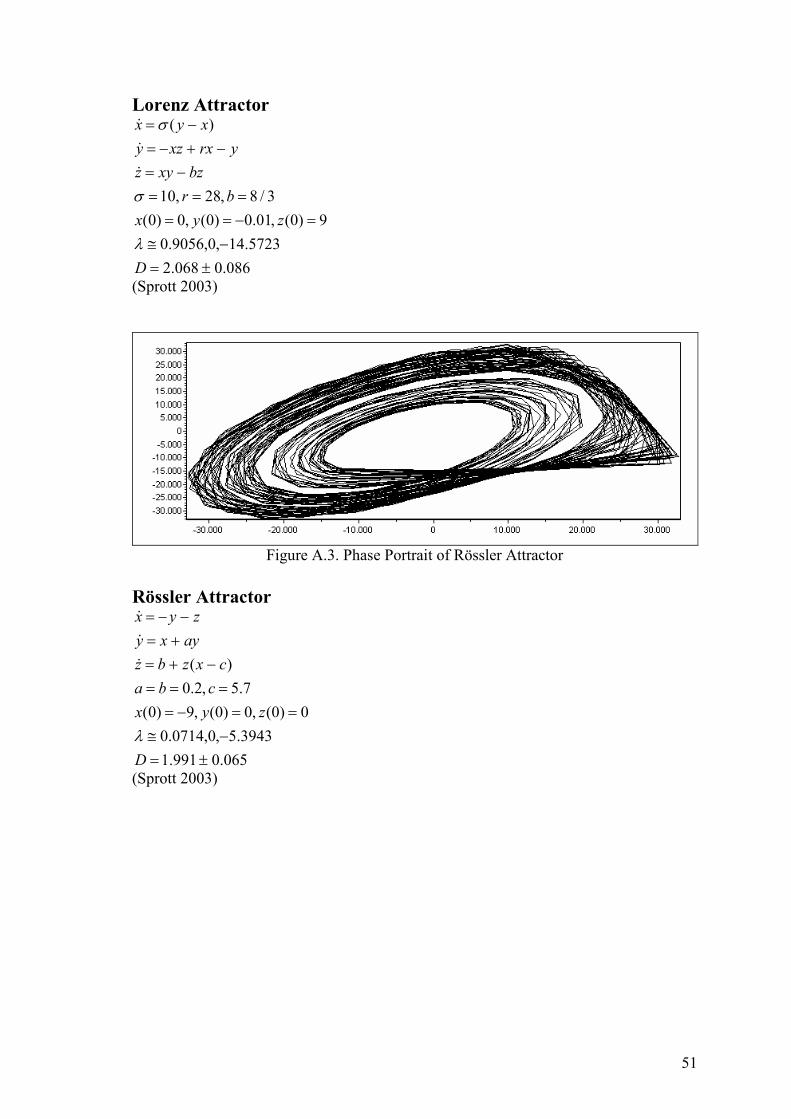
51
Lorenz Attractor
086.0068.2
5723.14,0,9056.0
9)0(,01.0)0(,0)0(
3/8,28,10
)(
±=
−≅
=−==
===
−=
−+−=
−=
D
zyx
br
bzxyz
yrxxzy
xyx
λ
σ
σ
&
&
&
(Sprott 2003)
Figure A.3. Phase Portrait of Rössler Attractor
Rössler Attractor
065.0991.1
3943.5,0,0714.0
0)0(,0)0(,9)0(
7.5,2.0
)(
±=
−≅
==−=
===
−+=
+=
−−=
D
zyx
cba
cxzbz
ayxy
zyx
λ
&
&
&
(Sprott 2003)

52
APPENDIX B
STATISTICAL PARAMETERS Root mean square (RMS)
Root mean square indicates the magnitude of variation of a series of discerete
values or a continuously varying function. The name comes from the process of RMS.
Firstly, the squares the values is taken. Then, mean of the squared values is found. And
finally, root of mean of the squared values is calculated.
∑=
=N
i
ixN 1
21RMS (B.1)
Skewness
Asymmetry in the distribution of the sample data values is called skewness.
There are two different tails of the distribution such as left tail having lower value of the
distribution and right tail having higher value of the distribution. If the left tail is longer,
then the function has negative skewness or left-skewed. On the other hand, if the right
tail is longer, then it has positive skewness or right-skewed. Generally, positive
skewness is more common than negative skewness.
Skew=2/322/3
1
3
))(()1(
)(1
∑
∑
−
−=
xxN
xxN
i
N
i
i
(B.2)
Kurtosis
If the sampled data is skewed, transformation can be applied to the data, for
example, taking logarithms of right-skewed data. Then, one can characterize the shape
of a distribution by using Kurtosis. If the tails are heavier then for a normal distribution,
then Kurtosis of the distribution is positive. Kurtosis of the distribution is negative
when the tail are lighter. Kurtosis of zero is possible for the normal distribution.

53
Kurtosis=222
1
4
))(()1(
)(1
∑
∑
−
−=
xxN
xxN
i
N
i
i
(B.3)
Crest factor
The Crest factor shows the ratio of the peak value of a waveform to its RMS
value . It is defined by a pure number without units. For example, the crest factor of a
sine wave is 1.414 when the peak value is 1.414 times the RMS value. A typical
vibration signals from an unbalanced machine without any other problems have a nearly
1.5 crest factor. But when the bearings begin to wear, and impacting begins, the crest
factor becomes much greater than this. The crest factor is so sensitive to the sharp peaks
in the waveform. The reason of this is that the peaks happens suddenly, and hence it
does not contain very much energy.
Crest Factor=
RMS
peakmax (B.4)

54
APPENDIX C
CULPERTUS
Culpertus is a time series analyzing program which allows time series invariants
calculations and graphical representations. Culpertus takes its name from Latin letters
“culpa compertus” which means fault certain. Autocorrelation, correlation sum,
correlation dimension and metric entropy can be calculated with Culpertus. To
download culpertus, please visit http://www.iyte.edu.tr/~erhansevil/
Figure C.1. Culpertus Open file
Figure C.2. Culpertus Save Image

55
Figure C.3. Culpertus Autocorrelation
Figure C.4. Culpertus Correlation Sum Parameters

56
Figure C.5. Culpertus Chaotic Invariants