On the properties of equally-weightedrisk contributions portfolios∗

Sébastien Maillard† Thierry Roncalli‡ Jérôme Teiletche§

First version: June 2008 � This version: May 2009

AbstractMinimum variance and equally-weighted portfolios have recently prompted

great interest both from academic researchers and market practitioners, as theirconstruction does not rely on expected average returns and is therefore as-sumed to be robust. In this paper, we consider a related approach, where therisk contribution from each portfolio components is made equal, which maxi-mizes diversi�cation of risk (at least on an ex-ante basis). Roughly speaking,the resulting portfolio is similar to a minimum variance portfolio subject toa diversi�cation constraint on the weights of its components. We derive thetheoretical properties of such a portfolio and show that its volatility is locatedbetween those of minimum variance and equally-weighted portfolios. Empiricalapplications con�rm that ranking. All in all, equally-weighted risk contribu-tions portfolios appear to be an attractive alternative to minimum varianceand equally-weighted portfolios and might be considered a good trade-o� be-tween those two approaches in terms of absolute level of risk, risk budgetingand diversi�cation.

Keywords: Asset allocation, risk contributions, minimum-variance, portfolio con-struction, risk budgeting, portfolio diversi�cation.JEL classi�cation: G11, C60.

∗The authors thank Eric Bouyé, Benjamin Bruder, Thierry Michel, Florent Pochon, GuillaumeSabouret, Guillaume Weisang and, especially, Lionel Martellini and an anonymous referee for theirhelpful comments and suggestions.

†SGAM Alternative Investments, sebastien.maillard@sgam.com.‡SGAM Alternative Investments and University of Evry, thierry.roncalli@sgam.com.§Lombard Odier and University of Paris Dauphine, jerome.teiletche@dauphine.fr.

1

1 IntroductionOptimal portfolio construction, the process of e�ciently allocating wealth amongasset classes and securities, has a longstanding history in the academic literature.Over �fty years ago, Markowitz [1952, 1956] formalized the problem in a mean-variance framework where one assumes that the rational investor seeks to maximizethe expected return for a given volatility level. While powerful and elegant, thissolution is known to su�er from serious drawbacks in its practical implementation.First, optimal portfolios tend to be excessively concentrated in a limited subset of thefull set of assets or securities. Second, the mean-variance solution is overly sensitive tothe input parameters. Small changes in those parameters, most notably in expectedreturns (Merton [1980]), can lead to signi�cant variations in the composition of theportfolio.

Alternative methods to deal with these issues have been suggested in the lit-erature, such as portfolio resampling (Michaud [1989]) or robust asset allocation(Tütüncü and Koenig [2004]), but have their own disadvantages. On top of thoseshortcomings, is the additional computational burden which is forced upon investors,as they need to compute solutions across a large set of scenarios. Moreover, it can beshown that these approaches can be restated as shrinkage estimator problems (Jo-rion [1986]) and that their out-of-sample performance is not superior to traditionalones (Scherer [2007a, 2007b]). Looking at the marketplace, it also appears that alarge fraction of investors prefers more heuristic solutions, which are computationallysimple to implement and are presumed robust as they do not depend on expectedreturns.

Two well-known examples of such techniques are the minimum variance and theequally-weighted portfolios. The �rst one is a speci�c portfolio on the mean-variancee�cient frontier. Equity funds applying this principle have been launched in recentyears. This portfolio is easy to compute since the solution is unique. As the onlymean-variance e�cient portfolio not incorporating information on the expected re-turns as a criterion, it is also recognized as robust. However, minimum-varianceportfolios generally su�er from the drawback of portfolio concentration. A simpleand natural way to resolve this issue is to attribute the same weight to all the assetsconsidered for inclusion in the portfolio. Equally weighted or "1/n" portfolios arewidely used in practice (Bernartzi and Thaler [2001], Windcli� and Boyle [2004])and they have been shown to be e�cient out-of-sample (DeMiguel, Garlappi andUppal [2009]). In addition, if all assets have the same correlation coe�cient as wellas identical means and variances, the equally-weighted portfolio is the unique port-folio on the e�cient frontier. The drawback is that it can lead to a very limiteddiversi�cation of risks if individual risks are signi�cantly di�erent.

In this paper, we analyze another heuristic approach, which constitutes a middle-ground stemming between minimum variance and equally-weighted portfolios. The

2

idea is to equalize risk contributions from the di�erent components of the portfolio1.The risk contribution of a component i is the share of total portfolio risk attributableto that component. It is computed as the product of the allocation in componenti with its marginal risk contribution, the latter one being given by the change inthe total risk of the portfolio induced by an in�nitesimal increase in holdings ofcomponent i. Dealing with risk contributions has become standard practice forinstitutional investors, under the label of "risk budgeting". Risk budgeting is theanalysis of the portfolio in terms of risk contributions rather than in terms of portfolioweights. Qian [2006] has shown that risk contributions are not solely a mere (ex-ante) mathematical decomposition of risk, but that they have �nancial signi�canceas they can be deemed good predictors of the contribution of each position to (ex-post) losses, especially for those of large magnitude. Equalizing risk contributions isalso known as a standard practice for multistrategy hedge funds like CTAs althoughthey generally ignore the e�ect of correlation among strategies (more precisely, theyare implicitly making assumptions about homogeneity of the correlation structure).

Investigating the out-of-sample risk-reward properties of equally-weighted riskcontributions (ERC) portfolios is interesting because they mimic the diversificatione�ect of equally-weighted portfolios while taking into account single and joint riskcontributions of the assets. In other words, no asset contributes more than its peersto the total risk of the portfolio. The minimum-variance portfolio also equalizesrisk contributions, but only on a marginal basis. That is, for the minimum-varianceportfolio, a small increase in any asset will lead to the same increase in the totalrisk of the portfolio (at least on an ex-ante basis). Except in special cases, thetotal risk contributions of the various components will however be far from equal,so that in practice the investor often concentrates its risk in a limited number ofpositions, giving up the bene�t of diversification. It has been shown repeatedlythat the diversi�cation of risks can improve returns (Fernholtz et al. [1998], Boothand Fama [1992]). Another rationale for ERC portfolios is based on optimalityarguments, as Lindberg [2009] shows that the solution to Markowitz's continuoustime portfolio problem is given, when positive drift rates are considered in Brownianmotions governing stocks prices, by the equalization of quantities related to riskcontributions.

The ERC approach is not new and has been already exposed in some recentarticles (Neurich [2008], Qian [2005]). However, none of them is studying the globaltheoretical issues linked to the approach pursued here. Note that the Most-Diversi�edPortfolio (MDP) of Choueifaty and Coignard [2008] shares with the ERC portfolioa similar philosophy based on diversi�cation. But the two portfolios are generallydistinct, except when correlation coe�cient components is unique. We also discuss

1We have restricted ourselves to the volatility of the portfolio as risk measure. The ERC principlecan be applied to other risk measures as well. Theoretically, it is only necessary that the riskmeasure is linear-homogeneous in the weights, in order for the total risk of the portfolio to be fullydecomposed into components. Under some hypotheses, this is the case for Value at risk for instance(Hallerback [2003]).

3

the optimality of the ERC portfolio within the scope of the Maximum Sharpe Ratio(MSR) reinvestigated by Martellini [2008].

The structure of this paper is as follows. We �rst de�ne ERC portfolios andanalyze their theoretical properties. We then compare the ERC with competingapproaches and provide empirical illustrations. We �nally draw some conclusions.

2 De�nition of ERC portfolios2.1 De�nition of marginal and total risk contributionsWe consider a portfolio x = (x1, x2, ..., xn) of n risky assets. Let σ2

i be the variance ofasset i, σij be the covariance between assets i and j and Σ be the covariance matrix.Let σ (x) =

√x>Σx =

∑i x

2i σ

2i +

∑i

∑j 6=i xixjσij be the risk of the portfolio.

Marginal risk contributions, ∂xi σ (x), are de�ned as follows:

∂xi σ (x) =∂ σ (x)∂ xi

=xiσ

2i +

∑j 6=i xjσij

σ (x)

The adjective "marginal" quali�es the fact that those quantities give the change involatility of the portfolio induced by a small increase in the weight of one component.If one notes σi (x) = xi × ∂xiσ (x) the (total) risk contribution of the ith asset, thenone obtains the following decomposition1:

σ (x) =n∑

i=1

σi (x)

Thus the risk of the portfolio can be seen as the sum of the total risk contributions2.

2.2 Speci�cation of the ERC strategyStarting from the de�nition of the risk contribution σi (x), the idea of the ERCstrategy is to �nd a risk-balanced portfolio such that the risk contribution is thesame for all assets of the portfolio. We voluntary restrict ourselves to cases withoutshort selling, that is 0 ≤ x ≤ 1. One reason is that most investors cannot take shortpositions. Moreover, since our goal is to compare the ERC portfolios with otherheuristic approaches, it is important to keep similar constraints for all solutions tobe fair. Indeed, by construction the 1/n portfolio satis�es positive weights constraintand it is well-known that constrained portfolios are less optimal than unconstrainedones (Clarke et al., 2002). Mathematically, the problem can thus be written asfollows:

x? ={

x ∈ [0, 1]n :∑

xi = 1, xi × ∂xi σ (x) = xj × ∂xj σ (x) for all i, j}

(1)1The volatility σ is a homogeneous function of degree 1. It thus satis�es Euler's theorem and

can be reduced to the sum of its arguments multiplied by their �rst partial derivatives.2In vector form, noting Σ the covariance matrix of asset returns, the n marginal risk contributions

are computed as: Σx√x>Σx

. We verify that: x> Σx√x>Σx

=√

x>Σx = σ (x).

4

Using endnote 2 and noting that ∂xi σ (x) ∝ (Σx)i,the problem then becomes:

x? ={

x ∈ [0, 1]n :∑

xi = 1, xi × (Σx)i = xj × (Σx)j for all i, j}

(2)

where (Σx)i denotes the ith row of the vector issued from the product of Σ with x.

Note that the budget constraint∑

xi = 1 is only acting as a normalization one.In particular, if the portfolio y is such that yi× ∂yi σ (y) = yj × ∂yj σ (y) with yi ≥ 0but

∑yi 6= 1, then the portfolio x de�ned by xi = yi/

∑ni=1 yi is the ERC portfolio.

3 Theoretical properties of ERC portfolios3.1 The two-asset case (n = 2)

We begin by analyzing the ERC portfolio in the bivariate case. Let ρ be the correla-tion and x = (w, 1− w) the vector of weights. The vector of total risk contributionsis:

1σ (x)

(w2σ2

1 + w(1− w)ρσ1σ2

(1− w)2σ22 + w(1− w)ρσ1σ2

)

In this case, �nding the ERC portfolio means �nding w such that both rows are equal,that is w verifying w2σ2

1 = (1−w)2σ22. The unique solution satisfying 0 ≤ w ≤ 1 is:

x? =(

σ−11

σ−11 + σ−1

2

,σ−1

2

σ−11 + σ−1

2

)

Note that the solution does not depend on the correlation ρ.

3.2 The general case (n > 2)

In more general cases, where n > 2, the number of parameters increases quickly,with n individual volatilities and n(n− 1)/2 bivariate correlations.

Let us begin with a particular case where a simple analytic solution can beprovided. Assume that we have equal correlations for every couple of variables,that is ρi,j = ρ for all i, j. The total risk contribution of component i thus be-comes σi (x) =

(x2

i σ2i + ρ

∑j 6=i xixjσiσj

)/σ (x) which can be written as σi (x) =

xiσi

((1− ρ) xiσi + ρ

∑j xjσj

)/σ (x). The ERC portfolio being de�ned by σi (x) =

σj (x) for all i, j, some simple algebra shows that this is here equivalent3 to xiσi =xjσj . Coupled with the (normalizing) budget constraint

∑i xi = 1, we deduce that:

xi =σ−1

i∑nj=1 σ−1

j

(3)

3We use the fact that the constant correlation veri�es ρ ≥ − 1n−1

.

5

The weight allocated to each component i is given by the ratio of the inverse ofits volatility with the harmonic average of the volatilities. The higher (lower) thevolatility of a component, the lower (higher) its weight in the ERC portfolio.

In other cases, it is not possible to �nd explicit solutions of the ERC portfolio.Let us for example analyse the case where all volatilities are equal, σi = σ for all i,but where correlations di�er. By the same line of reasoning as in the case of constantcorrelation, we deduce that:

xi =(∑n

k=1 xkρik)−1

∑nj=1

(∑nk=1 xkρjk

)−1 (4)

The weight attributed to component i is equal to the ratio between the inverse ofthe weighted average of correlations of component i with other components andthe same average across all the components. Notice that contrary to the bivariatecase and to the case of constant correlation, for higher order problems, the solutionis endogenous since xi is a function of itself directly and through the constraintthat

∑i xi = 1. The same issue of endogeneity naturally arises in the general case

where both the volatilities and the correlations di�er. Starting from the de�nitionof the covariance of the returns of component i with the returns of the aggregatedportfolio, σix = cov

(ri,

∑j xjrj

)=

∑j xjσij , we have σi (x) = xiσix/σ (x). Now,

let us introduce the beta βi of component i with the portfolio. By de�nition, wehave βi = σix/σ2 (x) and σi (x) = xiβiσ (x) . The ERC portfolio being de�ned byσi (x) = σj (x) = σ (x) /n for all i, j, it follows that:

xi =β−1

i∑nj=1 β−1

j

=β−1

i

n(5)

The weight attributed to component i is inversely proportional to its beta. The higher(lower) the beta, the lower (higher) the weight, which means that components withhigh volatility or high correlation with other assets will be penalized. Recall thatthis solution is endogenous since xi is a function of the component beta βi which byde�nition depends on the portfolio x.

3.3 Numerical solutionsWhile the previous equations (4) and (5) allow for an interpretation of the ERCsolution in terms of the relative risk of an asset compared to the rest of the portfolio,because of the endogeneity of the program, it does not o�er a closed-form solution.Finding a solution thus requires the use of a numerical algorithm.

In this perspective, one approach is to solve the following optimization problemusing a SQP (Sequential Quadratic Programming) algorithm:

x? = arg min f (x) (6)u.c. 1>x = 1 and 0 ≤ x ≤ 1

6

where:

f (x) =n∑

i=1

n∑

j=1

(xi (Σx)i − xj (Σx)j

)2

The existence of the ERC portfolio is ensured only when the condition f (x?) = 0is veri�ed, i.e. xi (Σx)i = xj (Σx)j for all i, j. Basically, the program minimizes thevariance of the (rescaled) risk contributions.

An alternative to the previous algorithm is to consider the following optimizationproblem:

y? = arg min√

y>Σy (7)

u.c.{ ∑n

i=1 ln yi ≥ cy ≥ 0

with c an arbitrary constant. In this case, the program is similar to a variance min-imization problem subject to a constraint of su�cient diversi�cation of weights (asimplied by the �rst constraint), an issue to which we will be back below. This prob-lem may be solved using SQP. The ERC portfolio is expressed as x?

i = y∗i /∑n

i=1 y∗i(see Appendix A.2).

Our preference goes to the �rst optimization problem which is easier to solvenumerically since it does not incorporate a non-linear inequality constraint. Still,we were able to �nd examples where numerical optimization was tricky. If a nu-merical solution for the optimization problem (6) is not found, we recommend tomodify slightly this problem by the following: y? = arg min f (y) with y ≥ 0 and1>y ≥ c with c an arbitrary positive scalar. In this case, the ERC portfolio isx?

i = y∗i /∑n

i=1 y∗i for f (y?) = 0. This new optimization problem is easier to solvenumerically than (6) because the inequality constraint 1>y ≥ c is less restrictivethan the equality constraint 1>x = 1. On its side, the formulation in (7) has theadvantage that it allows to show that the ERC solution is unique as far as the covari-ance matrix Σ is positive-de�nite. Indeed, it is de�ning the minimization programof a quadratic function (a convex function) with a lower bound (itself a convex func-tion). Finally, one should notice that when relaxing the long-only constraint, varioussolutions satisfying the ERC condition can be obtained.

3.4 Comparison with 1/n and minimum-variance portfoliosAs stated in the introduction, 1/n and minimum-variance (MV) portfolios are widelyused in practice. ERC portfolios are naturally located between both and thus appearas good potential substitutes for these traditional approaches.

In the two-assets case, the 1/n portfolio is such that w∗1/n = 12 . It is thus only

when the volatilities of the two assets are equal, σ1 = σ2, that the 1/n and the ERC

7

portfolios coincide. For the minimum-variance portfolio, the unconstrained solutionis given by w∗mv =

(σ2

2 − ρσ1σ2

)/

(σ2

1 + σ22 − 2ρσ1σ2

). It is straightforward to show

that the minimum-variance portfolio coincide with the ERC one only for the equally-weighted portfolio where σ1 = σ2. For other values of σ1 and σ2, portfolio weightswill di�er.

In the general n-assets context, and a unique correlation, the 1/n portfolio isobtained as a particular case where all volatilities are equal. Moreover, we can showthat the ERC portfolio corresponds to the MV portfolio when cross-diversi�cation isthe highest (that is when the correlation matrix reaches its lowest possible value)4.This result suggests that the ERC strategy produces portfolios with robust risk-balanced properties.

Let us skip now to the general case. If we sum up the situations from the pointof view of mathematical de�nitions of these portfolios, they are as follows (wherewe use the fact that MV portfolios are equalizing marginal contributions to risk; seeScherer, 2007b):

xi = xj (1/n)∂xi σ (x) = ∂xj σ (x) (mv)xi∂xi σ (x) = xj∂xj σ (x) (erc)

Thus, ERC portfolios may be viewed as a portfolio located between the 1/n and theMV portfolios. To elaborate further this point of view, let us consider a modi�edversion of the optimization problem (7):

x? (c) = arg min√

x>Σx (8)

u.c.

∑ni=1 ln xi ≥ c

1>x = 1x ≥ 0

In order to get the ERC portfolio, one minimizes the volatility of the portfolio subjectto an additional constraint,

∑ni=1 lnxi ≥ c where c is a constant being determined

by the ERC portfolio. The constant c can be interpreted as the minimum levelof diversi�cation among components which is necessary in order to get the ERCportfolio5. Two polar cases can be de�ned with c = −∞ for which one gets the MVportfolio and c = −n ln n where one gets the 1/n portfolio. In particular, the quantity∑

lnxi, subject to∑

xi = 1, is maximized for xi = 1/n for all i. This reinforces theinterpretation of the ERC portfolio as an intermediary portfolio between the MV andthe 1/n ones, that is a form of variance-minimizing portfolio subject to a constraintof su�cient diversi�cation in terms of component weights. Finally, starting from this

4Proof of this result may be found in Appendix A.15In statistics, the quantity −Pxi ln xi is known as the entropy. For the analysis of portfolio

constructions using the maximum entropy principle, see Bera and Park [2008]. Notice however thatthe issue here studied is more speci�c.

8

new optimization program, we show in Appendix A.3 that volatilities are ordered inthe following way:

σmv ≤ σerc ≤ σ1/n

This means that we have a natural order of the volatilities of the portfolios, with theMV being, unsurprisingly, the less volatile, the 1/n being the more volatile and theERC located between both.

3.5 OptimalityIn this paragraph, we investigate when the ERC portfolio corresponds to the Maxi-mum Sharpe Ratio (MSR) portfolio, also known as the tangency portfolio in portfoliotheory, whose composition is equal to Σ−1(µ−r)

1>Σ−1(µ−r)where µ is the vector of expected

returns and r is the risk-free rate (Martellini, 2008). Scherer (2007b) shows that theMSR portfolio is de�ned as the one such that the ratio of the marginal excess returnto the marginal risk is the same for all assets constituting the portfolio and equalsthe Sharpe ratio of the portfolio:

µ (x)− r

σ (x)=

∂xµ (x)− r

∂xσ (x)

We deduce that the portfolio x is MSR if it veri�es the following relationship6:

µ− r =(

µ (x)− r

σ (x)

)Σx

σ (x)

We can show that the ERC portfolio is optimal if we assume a constant correlationmatrix and supposing that the assets have all the same Sharpe ratio. Indeed, with theconstant correlation coe�cient assumption, the total risk contribution of componenti is equal to (Σx)i /σ (x) . By de�nition, this risk contribution will be the same forall assets. In order to verify the previous condition, it is thus enough that eachasset posts the same individual Sharpe ratio, si = µi−r

σi. On the opposite, when

correlation will di�er or when assets have di�erent Sharpe ratio, the ERC portfoliowill be di�erent from the MSR one.

4 Illustrations4.1 A numerical exampleWe consider a universe of 4 risky assets. Volatilities are respectively 10%, 20%,30% and 40%. We �rst consider a constant correlation matrix. In the case of the1/n strategy, the weights are 25% for all the assets. The solution for the ERCportfolio is 48%, 24%, 16% and 12%. The solution for the MV portfolio depends onthe correlation coe�cient. With a correlation of 50%, the solution is xmv

1 = 100%.With a correlation of 30%, the solution becomes xmv

1 = 89.5% and xmv2 = 10.5%.

6Because we have µ (x) = x>µ, σ (x) =√

x>Σx, ∂xµ (x) = µ and ∂xσ (x) = Σx/σ (x).

9

When the correlation is 0%, we get xmv1 = 70.2%, xmv

2 = 17.6%, xmv3 = 7.8% and

xmv4 = 4.4%. Needless to say, the ERC portfolio is a portfolio more balanced in terms

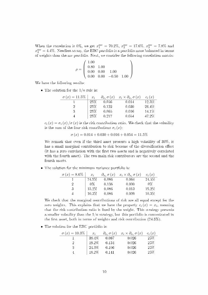
of weights than the mv portfolio. Next, we consider the following correlation matrix:

ρ =

1.000.80 1.000.00 0.00 1.000.00 0.00 −0.50 1.00

We have the following results:

• The solution for the 1/n rule is:σ (x) = 11.5% xi ∂xi σ (x) xi × ∂xi σ (x) ci (x)

1 25% 0.056 0.014 12.3%2 25% 0.122 0.030 26.4%3 25% 0.065 0.016 14.1%4 25% 0.217 0.054 47.2%

ci (x) = σi (x) /σ (x) is the risk contribution ratio. We check that the volatilityis the sum of the four risk contributions σi (x):

σ (x) = 0.014 + 0.030 + 0.016 + 0.054 = 11.5%

We remark that even if the third asset presents a high volatility of 30%, ithas a small marginal contribution to risk because of the diversi�cation e�ect(it has a zero correlation with the �rst two assets and is negatively correlatedwith the fourth asset). The two main risk contributors are the second and thefourth assets.

• The solution for the minimum variance portfolio is:σ (x) = 8.6% xi ∂xi σ (x) xi × ∂xi σ (x) ci (x)

1 74.5% 0.086 0.064 74.5%2 0% 0.138 0.000 0%3 15.2% 0.086 0.013 15.2%4 10.3% 0.086 0.009 10.3%

We check that the marginal contributions of risk are all equal except for thezero weights. This explains that we have the property ci (x) = xi, meaningthat the risk contribution ratio is �xed by the weight. This strategy presentsa smaller volatility than the 1/n strategy, but this portfolio is concentrated inthe �rst asset, both in terms of weights and risk contribution (74.5%).

• The solution for the ERC portfolio is:σ (x) = 10.3% xi ∂xi σ (x) xi × ∂xi σ (x) ci (x)

1 38.4% 0.067 0.026 25%2 19.2% 0.134 0.026 25%3 24.3% 0.106 0.026 25%4 18.2% 0.141 0.026 25%

10

Contrary to the minimum variance portfolio, the ERC portfolio is invested inall assets. Its volatility is bigger than the volatility of the MV but it is smallerthan the 1/n strategy. The weights are ranked in the same order for the ERCand MV portfolios but it is obvious that the ERC portfolio is more balancedin terms of risk contributions.

4.2 Real-life backtestsWe consider three illustrative examples. For all of these examples, we comparethe three strategies for building the portfolios 1/n, MV and ERC. We build thebacktests using a rolling-sample approach by rebalancing the portfolios every month(more precisely, the rebalancing dates correspond to the last trading day of themonth). For the MV and ERC portfolios, we estimate the covariance matrix usingdaily returns and a rolling window period of one year.

For each application, we compute the compound annual return, the volatilityand the corresponding Sharpe ratio (using the Fed fund as the risk-free rate) of thevarious methods for building the portfolio. We indicate the 1% Value-at-Risk andthe drawdown for the three holding periods: one day, one week and one month. Themaximum drawdown is also reported. We �nally compute some statistics measur-ing concentration, namely the Her�ndahl and the Gini indices, and turnover (seeAppendix A.4). In the tables of results, we present the average values of these con-centration statistics for both the weights (denoted as Hw and Gw respectively) andthe risk contributions (denoted as Hrc and Grc respectively). Regarding turnover,we indicate the average values of Tt across time. In general, we have preference forlow values of Ht, Gt and Tt. We now review the three sample applications.

Equity US sectors portfolioThe �rst example comes from the analysis of a panel of stock market sectoral indices.More precisely, we use the ten industry sectors for the US market as calculated byFTSE-Datastream. The sample period stems from January 1973 up to December2008. The list of sectors and basic descriptive statistics are given in Table 1. Duringthis period, sectoral indices have trended upward by 9% per year on average. Apartfrom two exceptions (Technologies on one side, Utilities on the other side), levels ofvolatilities are largely similar and tend to cluster around 19% per year. Correlationcoe�cients are �nally displayed in the remaining colums. The striking fact is thatthey stand out at high levels with only 3 among 45 below the 50% threshold. Allin all, this real-life example is characteristic of the case of similar volatilities andcorrelation coe�cients.

Backtests results are summarized in Table 2. The performance and risk statisticsof the ERC portfolio are very closed to their counterpart for the 1/n one, which isto be expected according to theoretical results when one considers the similarity involatilities and correlation coe�cients. Still, one noticeable di�erence between both

11

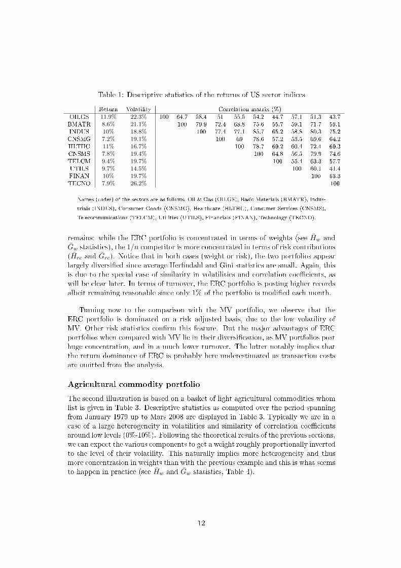
Table 1: Descriptive statistics of the returns of US sector indices

Return Volatility Correlation matrix (%)OILGS 11.9% 22.3% 100 64.7 58.4 51 55.5 54.2 44.7 57.1 51.3 43.7BMATR 8.6% 21.1% 100 79.9 72.4 68.8 75.6 55.7 59.1 71.7 59.1INDUS 10% 18.8% 100 77.4 77.1 85.7 65.2 58.8 80.3 75.2CNSMG 7.2% 19.1% 100 69 78.6 57.2 53.5 69.6 64.2HLTHC 11% 16.7% 100 78.7 60.2 60.4 72.4 60.3CNSMS 7.8% 19.4% 100 64.8 56.5 79.9 74.6TELCM 9.4% 19.7% 100 55.4 63.3 57.7UTILS 9.7% 14.5% 100 60.1 41.4FINAN 10% 19.7% 100 63.3TECNO 7.9% 26.2% 100

Names (codes) of the sectors are as follows: Oil & Gas (OILGS), Basic Materials (BMATR), Indus-trials (INDUS), Consumer Goods (CNSMG), Healthcare (HLTHC), Consumer Services (CNSMS),Telecommunications (TELCM), Utilities (UTILS), Financials (FINAN), Technology (TECNO).

remains: while the ERC portfolio is concentrated in terms of weights (see Hw andGw statistics), the 1/n competitor is more concentrated in terms of risk contributions(Hrc and Grc). Notice that in both cases (weight or risk), the two portfolios appearlargely diversi�ed since average Her�ndahl and Gini statistics are small. Again, thisis due to the special case of similarity in volatilities and correlation coe�cients, aswill be clear later. In terms of turnover, the ERC portfolio is posting higher recordsalbeit remaining reasonable since only 1% of the portfolio is modi�ed each month.

Turning now to the comparison with the MV portfolio, we observe that theERC portfolio is dominated on a risk adjusted basis, due to the low volatility ofMV. Other risk statistics con�rm this feature. But the major advantages of ERCportfolios when compared with MV lie in their diversi�cation, as MV portfolios posthuge concentration, and in a much lower turnover. The latter notably implies thatthe return dominance of ERC is probably here underestimated as transaction costsare omitted from the analysis.

Agricultural commodity portfolioThe second illustration is based on a basket of light agricultural commodities whomlist is given in Table 3. Descriptive statistics as computed over the period spanningfrom January 1979 up to Mars 2008 are displayed in Table 3. Typically we are in acase of a large heterogeneity in volatilities and similarity of correlation coe�cientsaround low levels (0%-10%). Following the theoretical results of the previous sections,we can expect the various components to get a weight roughly proportionally invertedto the level of their volatility. This naturally implies more heterogeneity and thusmore concentration in weights than with the previous example and this is what seemsto happen in practice (see Hw and Gw statistics, Table 4).

12

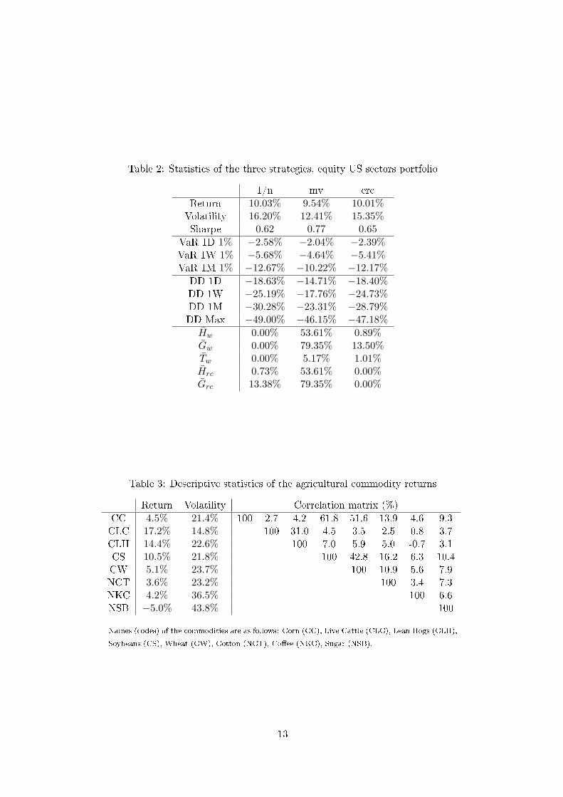
Table 2: Statistics of the three strategies, equity US sectors portfolio

1/n mv ercReturn 10.03% 9.54% 10.01%Volatility 16.20% 12.41% 15.35%Sharpe 0.62 0.77 0.65

VaR 1D 1% −2.58% −2.04% −2.39%VaR 1W 1% −5.68% −4.64% −5.41%VaR 1M 1% −12.67% −10.22% −12.17%

DD 1D −18.63% −14.71% −18.40%DD 1W −25.19% −17.76% −24.73%DD 1M −30.28% −23.31% −28.79%DD Max −49.00% −46.15% −47.18%

Hw 0.00% 53.61% 0.89%Gw 0.00% 79.35% 13.50%Tw 0.00% 5.17% 1.01%Hrc 0.73% 53.61% 0.00%Grc 13.38% 79.35% 0.00%

Table 3: Descriptive statistics of the agricultural commodity returns

Return Volatility Correlation matrix (%)CC 4.5% 21.4% 100 2.7 4.2 61.8 51.6 13.9 4.6 9.3CLC 17.2% 14.8% 100 31.0 4.5 3.5 2.5 0.8 3.7CLH 14.4% 22.6% 100 7.0 5.9 5.0 -0.7 3.1CS 10.5% 21.8% 100 42.8 16.2 6.3 10.4CW 5.1% 23.7% 100 10.9 5.6 7.9NCT 3.6% 23.2% 100 3.4 7.3NKC 4.2% 36.5% 100 6.6NSB −5.0% 43.8% 100

Names (codes) of the commodities are as follows: Corn (CC), Live Cattle (CLC), Lean Hogs (CLH),Soybeans (CS), Wheat (CW), Cotton (NCT), Co�ee (NKC), Sugar (NSB).

13

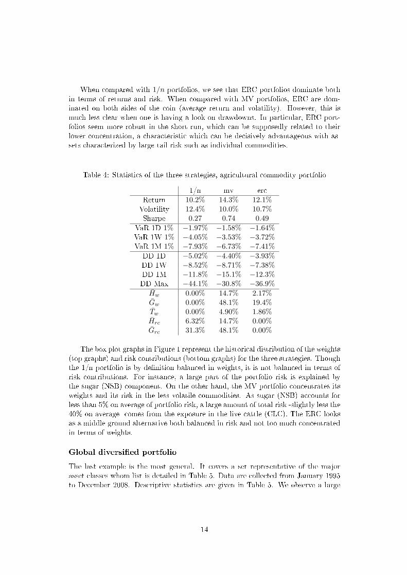
When compared with 1/n portfolios, we see that ERC portfolios dominate bothin terms of returns and risk. When compared with MV portfolios, ERC are dom-inated on both sides of the coin (average return and volatility). However, this ismuch less clear when one is having a look on drawdowns. In particular, ERC port-folios seem more robust in the short run, which can be supposedly related to theirlower concentration, a characteristic which can be decisively advantageous with as-sets characterized by large tail risk such as individual commodities.

Table 4: Statistics of the three strategies, agricultural commodity portfolio

1/n mv ercReturn 10.2% 14.3% 12.1%Volatility 12.4% 10.0% 10.7%Sharpe 0.27 0.74 0.49

VaR 1D 1% −1.97% −1.58% −1.64%VaR 1W 1% −4.05% −3.53% −3.72%VaR 1M 1% −7.93% −6.73% −7.41%

DD 1D −5.02% −4.40% −3.93%DD 1W −8.52% −8.71% −7.38%DD 1M −11.8% −15.1% −12.3%DD Max −44.1% −30.8% −36.9%

Hw 0.00% 14.7% 2.17%Gw 0.00% 48.1% 19.4%Tw 0.00% 4.90% 1.86%Hrc 6.32% 14.7% 0.00%Grc 31.3% 48.1% 0.00%

The box plot graphs in Figure 1 represent the historical distribution of the weights(top graphs) and risk contributions (bottom graphs) for the three strategies. Thoughthe 1/n portfolio is by de�nition balanced in weights, it is not balanced in terms ofrisk contributions. For instance, a large part of the portfolio risk is explained bythe sugar (NSB) component. On the other hand, the MV portfolio concentrates itsweights and its risk in the less volatile commodities. As sugar (NSB) accounts forless than 5% on average of portfolio risk, a large amount of total risk -slightly less the40% on average- comes from the exposure in the live cattle (CLC). The ERC looksas a middle-ground alternative both balanced in risk and not too much concentratedin terms of weights.

Global diversi�ed portfolioThe last example is the most general. It covers a set representative of the majorasset classes whom list is detailed in Table 5. Data are collected from January 1995to December 2008. Descriptive statistics are given in Table 5. We observe a large

14

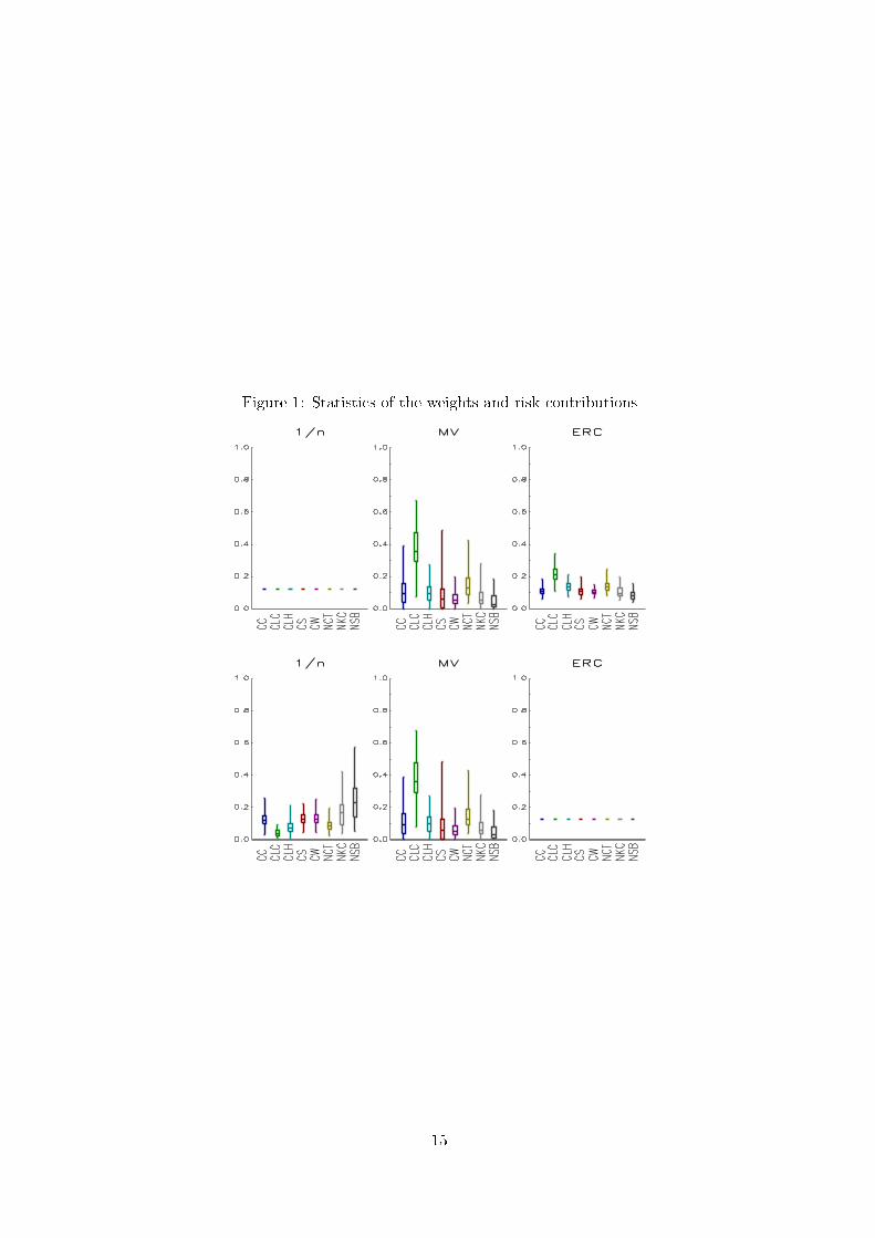
Figure 1: Statistics of the weights and risk contributions

15

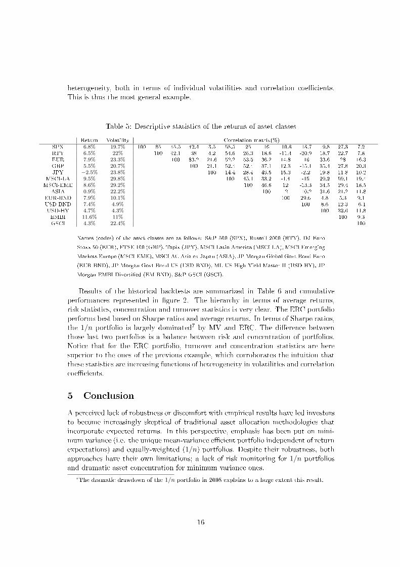
heterogeneity, both in terms of individual volatilities and correlation coe�cients.This is thus the most general example.

Table 5: Descriptive statistics of the returns of asset classesReturn Volatility Correlation matrix(%)

SPX 6.8% 19.7% 100 85 45.5 42.4 3.5 58.5 25 16 -10.8 -18.7 19.8 27.3 7.2RTY 6.5% 22% 100 42.1 38 4.2 54.6 26.3 18.6 -11.4 -20.9 18.7 22.7 7.8EUR 7.9% 23.3% 100 83.2 21.6 52.2 53.5 36.2 14.8 -16 33.6 28 16.3GBP 5.5% 20.7% 100 21.1 52.4 52.4 37.1 12.3 -15.1 35.4 27.8 20.3JPY −2.5% 23.8% 100 14.4 28.4 49.5 15.3 -2.2 19.8 11.8 10.2

MSCI-LA 9.5% 29.8% 100 45.1 33.2 -1.4 -15 29.2 59.1 19.4MSCI-EME 8.6% 29.2% 100 46.6 12 -13.3 34.5 29.4 18.5

ASIA 0.9% 22.2% 100 -2 -10.2 31.6 21.2 11.8EUR-BND 7.9% 10.1% 100 29.6 4.8 5.3 9.1USD-BND 7.4% 4.9% 100 8.6 12.3 -6.1USD-HY 4.7% 4.3% 100 32.6 11.8EMBI 11.6% 11% 100 9.3GSCI 4.3% 22.4% 100

Names (codes) of the asset classes are as follows: S&P 500 (SPX), Russell 2000 (RTY), DJ EuroStoxx 50 (EUR), FTSE 100 (GBP), Topix (JPY), MSCI Latin America (MSCI-LA), MSCI EmergingMarkets Europe (MSCI-EME), MSCI AC Asia ex Japan (ASIA), JP Morgan Global Govt Bond Euro(EUR-BND), JP Morgan Govt Bond US (USD-BND), ML US High Yield Master II (USD-HY), JPMorgan EMBI Diversi�ed (EM-BND), S&P GSCI (GSCI).

Results of the historical backtests are summarized in Table 6 and cumulativeperformances represented in �gure 2. The hierarchy in terms of average returns,risk statistics, concentration and turnover statistics is very clear. The ERC portfolioperforms best based on Sharpe ratios and average returns. In terms of Sharpe ratios,the 1/n portfolio is largely dominated7 by MV and ERC. The di�erence betweenthose last two portfolios is a balance between risk and concentration of portfolios.Notice that for the ERC portfolio, turnover and concentration statistics are heresuperior to the ones of the previous example, which corroborates the intuition thatthese statistics are increasing functions of heterogeneity in volatilities and correlationcoe�cients.

5 ConclusionA perceived lack of robustness or discomfort with empirical results have led investorsto become increasingly skeptical of traditional asset allocation methodologies thatincorporate expected returns. In this perspective, emphasis has been put on mini-mum variance (i.e. the unique mean-variance e�cient portfolio independent of returnexpectations) and equally-weighted (1/n) portfolios. Despite their robustness, bothapproaches have their own limitations; a lack of risk monitoring for 1/n portfoliosand dramatic asset concentration for minimum variance ones.

7The dramatic drawdown of the 1/n portfolio in 2008 explains to a large extent this result.

16

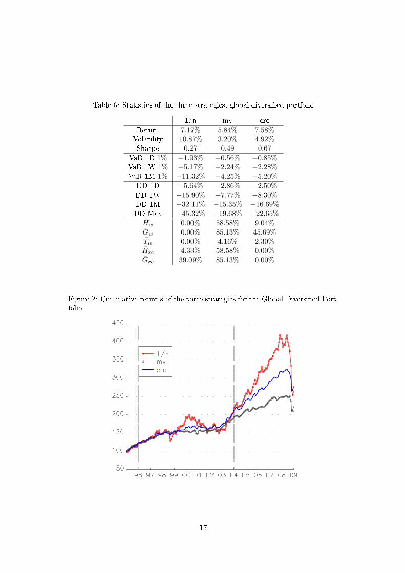
Table 6: Statistics of the three strategies, global diversi�ed portfolio

1/n mv ercReturn 7.17% 5.84% 7.58%Volatility 10.87% 3.20% 4.92%Sharpe 0.27 0.49 0.67

VaR 1D 1% −1.93% −0.56% −0.85%VaR 1W 1% −5.17% −2.24% −2.28%VaR 1M 1% −11.32% −4.25% −5.20%

DD 1D −5.64% −2.86% −2.50%DD 1W −15.90% −7.77% −8.30%DD 1M −32.11% −15.35% −16.69%DD Max −45.32% −19.68% −22.65%

Hw 0.00% 58.58% 9.04%Gw 0.00% 85.13% 45.69%Tw 0.00% 4.16% 2.30%Hrc 4.33% 58.58% 0.00%Grc 39.09% 85.13% 0.00%

Figure 2: Cumulative returns of the three strategies for the Global Diversi�ed Port-folio

17

We propose an alternative approach based on equalizing risk contributions fromthe various components of the portfolio. This way, we try to maximize dispersionof risks, applying some kind of �1/n� �lter in terms of risk. It constitutes a specialform of risk budgeting where the asset allocator is distributing the same risk budgetto each component, so that none is dominating (at least on an ex-ante basis). Thismiddle-ground positioning is particularly clear when one is looking at the hierarchyof volatilities. We have derived closed-form solutions for special cases, such as whena unique correlation coe�cient is shared by all assets. However, numerical opti-mization is necessary in most cases due to the endogeneity of the solutions. All inall, determining the ERC solution for a large portfolio might be a computationally-intensive task, something to keep in mind when compared with the minimum vari-ance and, even more, with the 1/n competitors. Empirical applications show thatequally-weighted portfolios are inferior in terms of performance and for any measureof risk. Minimum variance portfolios might achieve higher Sharpe ratios due to lowervolatility but they can expose to higher drawdowns in the short run. They are alsoalways much more concentrated and appear largely less e�cient in terms of portfolioturnover.

Empirical applications could be pursued in various ways. One of the most promis-ing would consist in comparing the behavior of equally-weighted risk contributionsportfolios with other weighting methods for major stock indices. For instance, inthe case of the S&P 500 index, competing methodologies are already commercializedsuch as capitalization-weighted, equally-weighted, fundamentally-weighted (Arnottet al. [2005]) and minimum-variance weighted (Clarke et al. [2002]) portfolios. Theway ERC portfolios would compare with these approaches for this type of equityindices remains an interesting open question.

18

References[1] Arnott, R., Hsu J. and Moore P. (2005), Fundamental indexation, Financial

Analysts Journal, 61(2), pp. 83-99

[2] Benartzi S. and Thaler R.H. (2001), Naive diversi�cation strategies in de-�ned contribution saving plans, American Economic Review, 91(1), pp. 79-98.

[3] Booth D. and Fama E. (1992), Diversi�cation and asset contributions, Finan-cial Analyst Journal, 48(3), pp. 26-32.

[4] Bera A. and Park S. (2008), Optimal portfolio diversi�cation using the max-imum entropy principle, Econometric Reviews, 27(4-6), pp. 484-512.

[5] Choueifaty Y. and Coignard Y. (2008), Towards maximum diversi�cation,Journal of Portfolio Management, 34(4), pp. 40-51.

[6] Clarke R., de Silva H. and Thorley S. (2002), Portfolio constraints and thefundamental law of active management, Financial Analysts Journal, 58(5), pp.48-66.

[7] Clarke R., de Silva H. and Thorley S. (2006), Minimum-variance portfoliosin the U.S. equity market, Journal of Portfolio Management, 33(1), pp. 10-24.

[8] DeMiguel V., Garlappi L. and Uppal R. (2009), Optimal Versus Naive Di-versi�cation: How Ine�cient is the 1/N Portfolio Strategy?, Review of FinancialStudies, 22, pp. 1915-1953.

[9] Estrada J. (2008), Fundamental indexation and international diversi�cation,Journal of Portfolio Management, 34(3), pp. 93-109.

[10] Fernholtz R., Garvy R. and Hannon J. (1998), Diversity-Weighted index-ing, Journal of Portfolio Management, 4(2), pp. 74-82.

[11] Hallerbach W. (2003), Decomposing portfolio Value-at-Risk: A general anal-ysis, Journal of Risk, 5(2), pp. 1-18.

[12] Jorion P. (1986), Bayes-Stein estimation for portfolio analysis, Journal of Fi-nancial and Quantitative Analysis, 21, pp. 293-305.

[13] Lindberg C. (2009), Portfolio optimization when expected stock returns aredetermined by exposure to risk, Bernouilli, forthcoming.

[14] Markowitz H.M. (1952), Portfolio selection, Journal of Finance, 7, pp. 77-91.

[15] Markowitz H.M. (1956), The optimization of a quadratic function subjet tolinear constraints, Naval research logistics Quarterly, 3, pp. 111-133.

[16] Markowitz H.M. (1959), Portfolio Selection: E�cient Diversi�cation of In-vestments, Cowles Foundation Monograph 16, New York.

19

[17] Martellini L. (2008), Toward the design of better equity benchmarks, Journalof Portfolio Management, 34(4), pp. 1-8.

[18] Merton R.C. (1980), On estimating the expected return on the market: Anexploratory investigation, Journal of Financial Economics, 8, pp. 323-361.

[19] Michaud R. (1989), The Markowitz optimization enigma: Is optimized opti-mal?, Financial Analysts Journal, 45, pp. 31-42.

[20] Neurich Q. (2008), Alternative indexing with the MSCI World Index, SSRN,April.

[21] Qian E. (2005), Risk parity portfolios: E�cient portfolios through true diver-si�cation, Panagora Asset Management, September.

[22] Qian E. (2006), On the �nancial interpretation of risk contributions: Risk bud-gets do add up, Journal of Investment Management, Fourth Quarter.

[23] Scherer B. (2007a), Can robust portfolio optimisation help to build betterportfolios?, Journal of Asset Management, 7(6), pp. 374-387.

[24] Scherer B. (2007b), Portfolio Construction & Risk Budgeting, Riskbooks,Third Edition.

[25] Tütüncü R.H and Koenig M. (2004), Robust asset allocation, Annals of Op-erations Research, 132, pp. 132-157.

[26] Windcliff H. and Boyle P. (2004), The 1/n pension plan puzzle, North Amer-ican Actuarial Journal, 8, pp. 32-45.

20

A AppendixA.1 The MV portfolio with constant correlationLet R = Cn (ρ) be the constant correlation matrix. We have Ri,j = ρ if i 6= j andRi,i = 1. We may write the covariance matrix as follows: Σ = σσ> ¯ R. We haveΣ−1 = Γ¯R−1 with Γi,j = 1

σiσjand

R−1 =ρ11> − ((n− 1) ρ + 1) I

(n− 1) ρ2 − (n− 2) ρ− 1.

With these expressions and by noting that tr (AB) = tr (BA), we may compute theMV solution x =

(Σ−11

)/1>Σ−11. We have:

xi =− ((n− 1) ρ + 1)σ−2

i + ρ∑n

j=1 (σiσj)−1

∑nk=1

(− ((n− 1) ρ + 1)σ−2

k + ρ∑n

j=1 (σkσj)−1

) .

Let us consider the lower bound of Cn (ρ) which is achieved for ρ = − (n− 1)−1. Itcomes that the solution becomes:

xi =

∑nj=1 (σiσj)

−1

∑nk=1

∑nj=1 (σkσj)

−1 =σ−1

i∑nk=1 σ−1

k

.

This solution is exactly the solution of the ERC portfolio in the case of constantcorrelation. This means that the ERC portfolio is similar to the MV portfolio whenthe unique correlation is at its lowest possible value.

A.2 On the relationship between the optimization problem (7) andthe ERC portfolio

The Lagrangian function of the optimization problem (7) is:

f (y;λ, λc) =√

y>Σy − λ>y − λc

(n∑

i=1

ln yi − c

)

The solution y? veri�es the following �rst-order condition:

∂yi (y;λ, λc) = ∂yi σ (y)− λi − λcy−1i = 0

and the Kuhn-Tucker conditions:{

min (λi, yi) = 0min (λc,

∑ni=1 ln yi − c) = 0

Because ln yi is not de�ned for yi = 0, it comes that yi > 0 and λi = 0. We noticethat the constraint

∑ni=1 ln yi = c is necessarily reached (because the solution can

not be y? = 0), then λc > 0 and we have:

yi∂ σ (y)∂ yi

= λc

21

We verify that risk contributions are the same for all assets. Moreover, we remarkthat we face a well know optimization problem (minimizing a quadratic functionsubject to lower convex bounds) which has a solution. We then deduce the ERCportfolio by normalizing the solution y? such that the sum of weights equals one.Notice that the solution x? may be found directly from the optimization problem (8)by using a constant c? = c− n ln (

∑ni=1 y?

i ) where c is the constant used to �nd y?.

A.3 On the relationship between σerc, σ1/n and σmv

Let us start with the optimization problem (8) considered in the body part of thetext:

x? (c) = arg min√

x>Σx

u.c.

∑ni=1 ln xi ≥ c

1>x = 10 ≤ x ≤ 1

We remark that if c1 ≤ c2, we have σ (x? (c1)) ≤ σ (x? (c2)) because the constraint∑ni=1 lnxi − c ≥ 0 is less restrictive with c1 than with c2. We notice that if c =

−∞, the optimization problem is exactly the MV problem, and x? (−∞) is the MVportfolio. Because of the Jensen inequality and the constraint

∑ni=1 xi = 1, we have∑n

i=1 lnxi ≤ −n ln n. The only solution for c = −n ln n is x?i = 1/n, that is the 1/n

portfolio. It comes that the solution for the general problem with c ∈ [−∞,−n lnn]satis�es:

σ (x? (−∞)) ≤ σ (x? (c)) ≤ σ (x? (−n ln n))

or:σmv ≤ σ (x? (c)) ≤ σ1/n

Using the result of Appendix 1, it exists a constant c? such that x? (c?) is the ERCportfolio. It proves that the inequality holds:

σmv ≤ σerc ≤ σ1/n

A.4 Concentration and turnover statisticsThe concentration of the portfolio is computed using the Her�ndahl and the Giniindices. Let xt,i be the weights of the asset i for a given month t. The de�nition ofthe Her�ndahl index is :

ht =n∑

i=1

x2t,i,

with xt,i ∈ [0, 1] and∑

i xt,i = 1. This index takes the value 1 for a perfectlyconcentrated portfolio (i.e., where only one component is invested) and 1/n for aportfolio with uniform weights. To scale the statistics onto [0, 1], we consider themodi�ed Her�ndahl index :

Ht =ht − 1/n

1− 1/n.

22

The Gini index G is a measure of dispersion using the Lorenz curve. Let X be arandom variable on [0, 1] with distribution function F . Mathematically, the Lorenzcurve is :

L (x) =

∫ x0 θ dF (θ)∫ 10 θ dF (θ)

If all the weights are uniform, the Lorenz curve is a straight diagonal line in the(x, L (x)) called the line of equality. If there is any inequality in size, then theLorenz curve falls below the line of equality. The total amount of inequality can besummarized by the Gini index which is computed by the following formula:

G = 1− 2∫ 1

0L (x) dx.

Like the modi�ed Her�ndahl index, it takes the value 1 for a perfectly concentratedportfolio and 0 for the portfolio with uniform weights. In order to get a feeling ofdiversi�cation of risks, we also apply concentration statistics to risk contributions.In the tables of results, we present the average values of these concentration statisticsfor both the weights (denoted as Hw and Gw respectively) and the risk contributions(denoted as Hrc and Grc respectively).

We �nally analyze the turnover of the portfolio. We compute it between twoconsecutive rebalancing dates with the following formula:

Tt =n∑

i=1

|xt,i − xt−1,i|2

.

Notice that this de�nition of turnover implies by construction a value of zero for the1/n portfolio while in practice, one needs to execute trades in order to rebalance theportfolio towards the 1/n target. However, apart in special circumstances, this e�ectis of second order and we prefer to concentrate on modi�cations of the portfolioinduced by active management decisions.In the tables of results, we indicate theaverage values of Tt across time. In general, we have preference for low values of Ht,Gt and Tt.

23