On the quantum Landau collision operator and electron ... · On the quantum Landau collision operator and electron collisions in dense plasmas Jer! ^ome Daligaulta) Theoretical Division,

On the quantum Landau collision operator and electron collisions in denseplasmas

J!erome Daligaulta)

Theoretical Division, Los Alamos National Laboratory, Los Alamos, New Mexico 87545, USA

(Received 5 February 2016; accepted 4 March 2016; published online 22 March 2016)

The quantum Landau collision operator, which extends the widely used Landau/Fokker-Planckcollision operator to include quantum statistical effects, is discussed. The quantum extension canserve as a reference model for including electron collisions in non-equilibrium dense plasmas, inwhich the quantum nature of electrons cannot be neglected. In this paper, the properties of theLandau collision operator that have been useful in traditional plasma kinetic theory and plasmatransport theory are extended to the quantum case. We outline basic properties in connection withthe conservation laws, the H-theorem, and the global and local equilibrium distributions. Wediscuss the Fokker-Planck form of the operator in terms of three potentials that extend the usualtwo Rosenbluth potentials. We establish practical closed-form expressions for these potentialsunder local thermal equilibrium conditions in terms of Fermi-Dirac and Bose-Einstein integrals.We study the properties of linearized quantum Landau operator, and extend two popularapproximations used in plasma physics to include collisions in kinetic simulations. We applythe quantum Landau operator to the classic test-particle problem to illustrate the physical effectsembodied in the quantum extension. We present useful closed-form expressions for theelectron-ion momentum and energy transfer rates. Throughout the paper, similarities and differen-ces between the quantum and classical Landau collision operators are emphasized. VC 2016AIP Publishing LLC. [http://dx.doi.org/10.1063/1.4944392]

I. INTRODUCTION

The work presented in this paper is part of an effort aimedat developing practical approximations to enable kinetic simu-lations of dense plasmas under non-equilibrium conditions.This is motivated by recent experiments on warm dense mat-ter and on charged-particle transport in plasmas formed alongthe compression pathway to ignition in inertial confinementfusion experiments. Indeed, by their nature, warm dense mat-ter experiments produce transient, non-equilibrium conditions,and measurements of equilibrium properties may be mislead-ing if recorded while the plasma species are still out of equi-librium.1 On the other hand, it is likely that current and futureX-ray diagnostics offer the possibility to probe the return toequilibrium of the non-equilibrium states thus created, andprovide new information on the nature of interactions in warmdense matter.2–4 Other recent experiments aimed at measuringthe stopping power of charged projectiles in inertial fusiontargets5 and warm dense matter,6,7 as well as alternativeparticle-beam inertial fusion designs,8 can also benefit fromnon-equilibrium kinetic simulations.

Unlike traditional plasmas, dense plasmas are denseenough and cold enough that the wave-like and fermionic na-ture of electrons can no longer be neglected. A major challengeto performing non-equilibrium simulations of dense plasmas isto include the quantum nature of conduction electrons in theircollisions among themselves and with ions. The state of theart computational methods for modeling dense plasmas isfinite-temperature density-functional-theory-based molecular

dynamics and quantum Monte-Carlo,9 which, by construction,represent well the electron-electron and electron-ion correla-tions in thermal equilibrium. However, electrons are not dy-namical in these approaches. As a consequence of thefluctuation-dissipation theorem, it is possible to extract lineartransport coefficients like the electrical conductivities fromthese simulations. However, transient dynamics, time-dependent disturbances, and non-equilibrium dynamics beyondthe linear regime are not accessible using these methods. Theextension of these microscopic methods, e.g., time-dependentdensity functional theory, to such dynamical conditions is stillin its infancy.9,10 Until now, the majority of non-equilibriumcalculations have been done using classical molecular dynam-ics, in which quantum effects are included through modifica-tions of the pair potentials used in the classical Newton’sequations of motion.11,12 Another approach, which is the preva-lent approach in traditional plasma physics, consists of describ-ing electrons with a kinetic equation that describes theevolution of the electron distribution function in phase-space.While quantum kinetic theory is a mature field,13,14 detailedquantum kinetic equations remain hard to solve both analyti-cally and numerically. This is true not only of the Kadanoff-Baym equations for the non-equilibrium Green’s functions butalso of less detailed descriptions like the quantum Boltzmannequation first introduced by Uehling and Uhlenbeck to extendthe celebrated Boltzmann equation to the quantum realm.13,15

In fact, similar remarks can be made about the inclusionof collisions in classical plasma physics. While fairly detailedkinetic theories exist, e.g., the Lenard-Balescu kinetic equa-tion, the simpler kinetic equation derived by Landau is gener-ally preferred in applications.16,17 The Landau equation or,a)Electronic mail: [email protected]

1070-664X/2016/23(3)/032706/22/$30.00 VC 2016 AIP Publishing LLC23, 032706-1

PHYSICS OF PLASMAS 23, 032706 (2016)

Reuse of AIP Publishing content is subject to the terms at: https://publishing.aip.org/authors/rights-and-permissions. Downloaded to IP: 192.12.184.6 On: Tue, 22 Mar2016 15:05:36

http://dx.doi.org/10.1063/1.4944392

http://dx.doi.org/10.1063/1.4944392

http://dx.doi.org/10.1063/1.4944392

mailto:[email protected]

http://crossmark.crossref.org/dialog/?doi=10.1063/1.4944392&domain=pdf&date_stamp=2016-03-22

equivalently, the Fokker-Plank operator is, indeed, the startingpoint or the underlying model of collisions of a large majorityof studies in many areas of plasma physics. There, the under-lying plasmas are typically hot and dilute enough that the av-erage particle kinetic energy greatly exceeds the potentialenergy of interaction. In this weakly coupled regime, colli-sions, i.e., the interactions of charged particles with theelectric and magnetic field fluctuations, cause only smalldeflections of the velocity vector of plasma particles. Theeffect of these deflections on the one-particle distributionfunctions is well described by the Landau operator, which isessentially a diffusion operator in velocity space. Curiously,to our knowledge, the quantum extension of the Landau equa-tion has not been considered as a suitable model of electroncollisions in dense plasmas. Under dense plasma conditionssuch as created in high-energy-density experiments, ions areweakly coupled at high enough temperature but becomestrongly coupled for temperatures below which their mean ki-netic energy is lower than their mean potential energy ofinteraction; the description of ion collisions with the Landaucolllision operator is invalid under such strongly coupled con-ditions. On the contrary, electrons remain weakly coupledamong themselves at all temperatures as a result of their fer-mionic character (higher kinetic energy states are being popu-lated as the temperature decreases). It is therefore legitimateto explore the possibility to model electron-electron interac-tions with a Landau-like collision operator that accounts forthe quantum nature of electrons. Like the classical Landau op-erator, the quantum Landau collision operator can be obtainedby retaining in the Boltzmann-Uehling-Uhlenbeck collisionintegral, only the small angle scattering events. To our knowl-edge, it was first introduced in the literature in 1980 byDanielewicz in the context of heavy-ion collision physics,but, apart from a few appearances in the mathematically ori-ented literature,18,19 it has not been utilized in physics. Likeits classical counterpart, this model of collisions is interestingsince it can be derived from controlled, physically motivatedapproximations; it incorporates important physics, includingthe effect of quantum degeneracy on the statistics of colli-sions; and it is more easily amenable to numerical simulationsthan other more detailed approximations. For these reasons,the quantum Landau collision operator is a relevant, non-trivial model of electron collisions in non-equilibrium densepalsmas, which can serve as a reference to more advanceddescriptions, in a way similar to the Thomas-Fermi modelwith respect to advanced density functional theory descrip-tions for equation-of-state calculations.

Our primary objective is to extend to the quantum casethe properties of the Landau collision operator that havebeen useful in traditional plasma kinetic theory and plasmatransport theory (see, e.g., Ref. 17). The extension is oftentechnically not straightforward, and we therefore give in theappendixes the details of the mathematical derivations andtricks used to this purpose. The resulting closed-form expres-sions highlighted in the main text, however, are easy to usein either analytical or numerical applications. In addition,throughout the paper, we emphasize the similarities and dif-ferences between the quantum and classical Landau collisionoperator. More precisely, the paper is organized as follows.

In Sec. II, the quantum Landau collision operator is intro-duced and its properties are studied. For completeness, wefirst recall important properties in connection with the con-servation laws, the H-theorem, and the global and local equi-librium distributions. We then express the quantum Landauoperator in the form of a non-linear Fokker-Planck operator.This requires introducing three Rosenbluth-like potentials,instead of two Rosenbluth potentials for the classical opera-tor. Practical, closed-form expressions of the potentials arethen given in the limit of local thermal equilibrium distribu-tion functions. We then illustrate the physical implications ofthe quantum corrections on the classic test-particle problemin an equilibrium electron-ion plasma; practical expressionsare given for the friction and diffusion coefficients and forthe energy loss rate of the test-particle. Finally, we presentuseful expressions for the electron-ion momentum andenergy transfer rates in plasmas consisting of quantum elec-trons and classical ions. In Sec. III, we extend the previousstudy to the linearized quantum Landau operator, linearizedaround local thermal equilibrium. This is motivated by thefact that linearized collision operators are central both in themathematical treatments of kinetic theories like in theChapman-Enskog method,20 and to some advanced numeri-cal algorithms like the df-method.21 In this regard, we extendto the quantum case two popular approximations of the line-arized collision operator that are used in traditional plasmakinetic simulations.

For convenience, the term quantum Landau-Fokker-Planck collision operator is used throughout the paper andabbreviated with the acronym qLFP to refer to the quantumLandau collision operator or to its Fokker-Planck form.

II. QUANTUM LANDAU COLLISION OPERATOR

To the best of our knowledge, the qLFP collision operatorwas first discussed by Danielewicz in Ref. 22 in the context ofheavy-ion collision physics. The operator was derived for gen-eral mutual interactions from the grazing collision approxima-tion of the Boltzmann-Uehling-Uhlenbeck kinetic equation.23

In the appendix of Ref. 22, the general collision operator wasspecialized to Coulomb interactions. For completeness, inAppendix A, we give a slightly different derivation startingfrom the Boltzmann-Uehling-Uhlenbeck collision operatorwith the dynamically screened Coulomb scattering cross sec-tion in the Born approximation. By construction, the qLFPcollision operator inherits the assumptions at the basis of theBoltzmann-Uehling-Uhlenbeck operator (e.g., regarding quan-tum exchange, and diffraction), and we refer the reader to theextensive literature on this equation for more details (in partic-ular, we recommend Ref. 13).

A. Definition

We consider a plasma consisting of N species of non-relativistic charged particles (including ions and electrons)of mass ma, charge qa ! Zae (e is minus the electron charge).Each species a is described by a single-particle phase-spacedistribution function fa"r; p; t#, normalized so that na"r; t# !!

dpfa"r; p; t# is the number density. For simplicity of exposi-tion of the properties of the qLFP collision operator, which

032706-2 J!erome Daligault Phys. Plasmas 23, 032706 (2016)


is the focus of this paper, we assume that collisions amongall species are described by a quantum Landau collision op-erator. In applications to dense plasmas, the qLFP kineticequation could be restricted to conduction electrons, whileanother description could be chosen to describe the ion dy-namics, in particular, under conditions when ions arestrongly coupled. Several schemes can be envisioned in thatrespect with different levels of sophistication. For instance, asimple model would describe both charged species withqLFP operators assuming classical ions and quantum elec-trons, and would include the effect of strong Coulomb cou-plings within the Coulomb logarithms, as is supported by therecently developed effective potential theory of trans-port.24–26 A more sophisticated approach would combine aqLFP treatment of the electrons with classical molecular dy-namics for the ions; the foundations of such a “kinetic theorymolecular dynamics” approach were recently discussed byGraziani et al.27

Within the Landau approximation, the distribution func-tions fa satisfy the kinetic equations

DfaDt!X

b

Cab fa; fb" #: (1)

Here

Dfa

Dt! @fa

@t$ pa

ma% @fa@r$ Fa %

@fa@pa

(2)

is the streaming operator describing the trajectories in phase-space of species a particles under the influence of the forceFa (e.g., the plasma mean electric field or an external disturb-ance). Cab"fa; fb# denotes the qLFP operator of interest in thispaper, which describes the effect on fa of collisions betweenparticles of species a with particles of species b (like-speciesscattering is described by the term with b! a). By droppingdependencies on "r; t#; Cab is given by

Cab fa; fb& ' pa" # ! cab @

@pa

%"

dpb V$

ab pa; pb" #

(

(@fa pa" #@pa

fb pb" # 1$ dbhbfb pb" ## $

)@fb pb" #@pb

fa pa" # 1$ dahafa pa" ## $

): (3)

Here,

cab ! 4pq2aq2

blablnKab;

where lnKab is the Coulomb logarithm (see below), and

V$

ab pa; pb" # !1

2labvabI$) vabvab

v2ab

% &;

where I$

is the identity tensor, lab ! mamb="ma $ mb# is thereduced mass, and

vab ! va ) vb; va !pa

ma:

In Eq. (3), da ! )1; 0; 1 for Fermi-Dirac, Boltzmann, andBose-Einstein statistics, respectively. The expression (3)includes the classical Landau equation as a special case bysetting da ! db ! 0. In the majority of applications inplasma physics, the ions can be treated as classical particlesda ! 0 and the electrons are fermions da ! )1. However,for sake of generality, the results presented below arederived irrespective of the particles’ statistics. Finally,

ha ! "2p"h#3ga

, where ga is the spin multiplicity factor of species

a (ga! 2 for electrons), so that drdp=ha is the number ofavailable states in the phase volume drdp.

B. Discussion

1. Quantum degeneracy effect

The bracket terms &1$ dahafa' and &1$ dbhbfb' in Cab

account for the quantum statistics. For fermions (da ! )1),

the Pauli principle requires that no more than drdpha

particles of

species a in the volume dr can possess momenta in the rangedp. The probability of a collision that would result in a parti-cle of species a entering this range is thus reduced in theratio &1) hafa'.28 For bosons, on the contrary, the presenceof a like particle in the range dp increases the probabilitythat a particle will enter that range in the ratio &1$ hafa'.

2. Coulomb logarithms

The Coulomb logarithm refers to the integral over mo-mentum transfers "hk

lnKab !"1

0

dk

k(4)

that arises in the process of retaining only the small-anglescattering events in the Boltzmann collision operator withthe Coulomb scattering law, or, as in Appendix A,

lnKab !"1

0

dk

k

1

! k; 0" #

''''

''''2

; (5)

when using the screened Coulomb scattering cross section inthe Born approximation (here ! is the total dielectric functionin the random phase approximation29). The integral (4) isdivergent at both ends of the integration range: at large mo-mentum transfer "hk, because of the grazing collisions approxi-mation, and at small k because of the infinite range of the bareCoulomb potential (the divergence is regularized by thedielectric function in Eq. (5)). In practice, physically moti-vated cutoff parameters kmin and kmax are introduced to regula-

rize the otherwise divergent integral, leading lnK ! ln kmaxkmin

( ).

We refer to Refs. 30 and 31 for detailed discussions on thechoice of cutoffs for dense plasmas, and to Appendix A ofRef. 32 for additional choices. For completeness, we recallhere the most popular prescription for typical dense electron-ion plasmas. The logarithm is expressed in the form30



lnK ! 1

2ln 1$ k2

max

k2min

!

;

with upper and lower cutoffs given as follows. The minimumkmin is set by Coulomb screening.33 For Kei

kmin ! min"ksc; 1=a#;

where ai ! "3=4pni#1=3 is the interionic distance and the ksc

is the inverse screening length

k2sc ! k2

D;i $ k2e ;

where kD;i is the ionic Debye length

k2D;i !

4pniq2i

kBTi;

and ke is the Thomas-Fermi screening length

k2e ! k2

D;e

Q)12

bele" #Q1

2bele" #

*k2

D;e

1$ T2F=T2

e

* +12

;

in terms of the Fermi-Dirac integral defined below. For Kee,kmin ! ke. The upper limit kmax is, under typical denseplasma conditions, set by the characteristic inverse electrondeBroglie wavelength of electrons, which is convenientlyapproximated across degeneracy regimes by

k2max !

24p

k2th

1$ T2F

T2e

!12

;

with kth !,,,,,,,,,,,,,,,,,,,,,,,,,,2p"h2=mekBTe

qthe thermal deBroglie wavelength.

3. Non-linearity

The quantum operator has a higher-order nonlinearitythan its classical counterpart, since the dependence on thedistribution functions is cubic in the quantum case andquadratic in the classical case. This leads to extra difficul-ties to deal with in both the analytical and numericaltreatments.

C. Properties

Like its classical counterpart,17 the qLFP collision oper-ator satisfies physically important properties in connectionwith the conservation laws and with the concept of irreversi-bility. These properties can be readily derived assuming thatthe distribution functions vanish sufficiently fast as jpj ! 1to eliminate surface integrals. Although these propertieshave already been discussed in Ref. 22, we recall them herewithout proof for the sake of completeness.

1. Local conservation laws

At each space-time point "r; t#, the total number of par-

ticles of any species na !!

dpfa, the total momentum

P !P

a

!dp pfa, and the total (kinetic) energy E !

Pa

!dp p2

2mafa are conserved by collisions. More precisely,

"dp Cab&fa; fb'"p# ! 0;

"dp p Cab&fa; fb'"p# ! )

"dp p Cba&fb; fa'"p#;

"dp

p2

2maCab fa; fb& ' p" # ! )

"dp

p2

2mbCba fb; fa& ' p" #;

i.e., the local density is not affected by collisions, the mo-mentum transfer rate from species b to species a is equal inmagnitude and opposite in direction to that from a to b, andthe energy is conserved in a binary collisions between spe-cies a and b.

2. H-theorem

Consider the total entropy density s and flux js definedas

s"r; t# ! )kB

X

a

"dp

ha

"faln"fa ) da 1$ da"fa

* +ln 1$ da

"fa* +# $

js"r; t#!)kB

X

a

"dp

ha

p

ma

"faln"fa)da 1$da"fa

* +ln 1$da

"fa

* +# $;

with "fa ! hafa. The qLFP kinetic equation implies

@s

@t$ @

@r% js + 0;

which expresses the local H-theorem. In particular, the totalentropy S"t# !

!drs"r; t# satisfies dS

dt + 0 and is a monotoni-cally increasing function of time, whatever the initialconditions.

3. Global equilibrium

As a consequence, whatever the initial conditions, thetime evolution reaches a final, time-independent state, a.k.a.stationary state, when S(t) reaches its maximum character-ized by dS

dt ! 0. The only stationary states are the Fermi-Dirac (da ! )1) or Bose-Einstein (da ! 1) distributionfunctions

fa r; p" # !1

ha

1

e)b&la) 12ma"p)mau#2' ) da

; 8a;

where the inverse temperature b ! 1=kBT, the chemicalpotential la, and the flow velocity u are constant independentof "r; t# and are the same for all species.

4. Local thermal equilibrium

The effect of collisions vanishes only when all speciesare in a local Fermi-Dirac or Bose-Einstein state at the same



local inverse temperature b"r; t# and flow velocity u"r; t#.More precisely,

Cab&fa; fb' ! 0 8a; b

if and only if, 8a,

fa r; p; t" # !1

ha

1

e)b r;t" # la r;t" #) 12ma

p)mau r;t" #" #2& ' ) da

: (6)

We recall for later reference that the classical limit of thelocal thermal equilibrium is given by bla ! )1, whichyields the familiar Maxwell-Boltzmann distribution

fa r; p; t" # , na r; t" #b

2pma

- .3=2

( e)b

2mapa)mau r;t" #& '2 for bla ! )1;

with the local number density na ! 1ha

2pmab

( )32ebla .

D. Fokker-Planck-like form of the quantumLandau-Fokker-Planck operator

The qLFP collision integral (3) can be written in theform of a non-linear Fokker-Planck collision operator34

Cab fa; fb& ' ! )@

@pa

%

"

Aabfa 1$ dahafa" # $ Babfa

) 1

2

@

@pa

% D$

abfa

( )#

; (7)

!) @

@pa

% Aabfa 1$ dahafa" #) 1

2D$

ab %@

@pa

fa

% &; (8)

where we introduced the “dynamical friction” vectors

Aab pa" # ! )cab

"dpb

@

@pb

% V$

ab pa; pb" #% &

fb pb" #;

Bab pa" # ! )mb

macab (

"dpb

@

@pb% V$

ab pa; pb" #% &

( fb pb" # 1$ dbhbfb pb" ## $

;

and the diffusion tensor

D$

ab"pa# ! 2cab

"dpbV

$

ab"pa; pb#fb"pb#&1$ dbhbfb"pb#':

For simplicity, we dropped the explicit dependences on "r; t#in the previous expressions. In deriving Eq. (8), we used the

relation Bab"pa# ! 12@@pa% D$

ab"pa#.As with the classical operator,35 the coefficients

Aab;Bab, and D$

ab can be written as

Aab pa" # !cab

mblab

@Hb va" #@va

; (9a)

Bab pa" # !cab

malab

@Ib va" #@va

; (9b)

D$

ab pa" # !cab

lab

@2Gb va" #@va@va

; (9c)

in terms of the three “potentials”

Hb v" # !"

dvb

~fb vb" #jv) vbj

;

Ib v" # !"

dvb

~fb vb" # 1$ db~hb

~fb vb" #h i

jv) vbj;

Gb v" # !"

dvbjv) vbj~fb vb" # 1$ db~hb

~fb vb" #h i

;

(10)

with ~hb - hb=m3b and ~f"vb# ! m3

bf "mbvb#. The three poten-tials Hb, Ib, and Gb are solution of Poisson’s equations

r2Hb"v# ! )4p~fb"v#;r2Ib"v# ! )4p~fb"v#&1$ db

~hb~fb"v#';

r2Gb"v# ! 2Ib"v#;

where r ! @@v.

In the case db ! 0; Bab"pa# ! mbma

Aab"pa#, and Eq. (7)corresponds to the usual Landau-Fokker-Planck collision op-erator with friction 1$ mb

ma

* +Aab. In this case, Ib!Hb, and Hb

and Gb reduce to the two usual Rosenbluth potentials.35

E. Potentials in local thermal equilibrium

We provide closed-form expressions for the potentialHb, Ib, and Gb when ~fb is a local equilibrium distributionfunction (6), i.e., (dropping the subscript b)

~f r; v; t" # !1~h

1

e)b r;t" # l r;t" #)m v)u r;t" #" #2=2& ' ) d:

These expressions are useful in a number of applications, includ-ing the test-particle problem and linear transport problem.

We recall that, in the classical case, the equilibriumRosenbluth potentials satisfy17,35

H v" # ! I v" # ! n

erf

,,,,,,,bm

2

rw

!

w; (11a)

G v" # ! n w$ 1

mbw

- .erf

,,,,,,,bm

2

rw

!

$

,,,,,,,,,2

pmb

s

e)bm2 w2

2

4

3

5;

(11b)

where w ! jv) uj. The extension of these expressions to thequantum case is not completely trivial, and we report thelengthy details in Appendix C. The results can be conven-iently expressed in terms of the usual Fermi-Dirac (d ! )1)and Bose-Einstein (d! 1) integrals of order " and argument tdefined as

Q" t" # ! 1

C " $ 1" #

"1

0

dyy"

ey)t ) d;



where C"t# !!1

0 xt)1e)xdx is the Gamma function, alongwith the lower incomplete integral defined as

Q" t; x" # !1

C " $ 1" #

"x

0

dyy"

ey)t ) d;

and the upper incomplete integral

Qc""t; x# ! Q""t# )Q""t; x#:

We find

H v" # !4pm2

bh

,,,pp

2,,,xp Q1=2 t; x" # $Qc

0 t; x" #

" #

; (12a)

I v" # !2m2p3=2

bh,,,xp Q)1

2t; x" #; (12b)

G v" # !4p3=2m

,,,xp

b2hQ)1

2t; x" # $

2p3=2m

b2h

1,,,xp Q1

2t; x" #

$ 8pm

b2hln 1$ e t)x" #* +

; (12c)

where t ! bl and x ! bmw2

2 . In the classical limit bl! )1,the previous expressions reduce to the classical Rosenbluthpotentials (11). This can be shown using

Q12

t; x" # , eterf,,,xp* +) 2

,,,xp,,,pp et)x

Q)12

t; x" # , eterf,,,xp* +

Qc0"t; x# , et)x

for t! )1. In practice, the potentials can be numericallyevaluated using accurate series representations of the inte-grals Q" , e.g., Ref. 36.

F. Scattering of a test-particle

In order to illustrate the effect of the quantum statisticson the Landau collision operator, we apply the previousresults to the classic test-particle problem. We consider a clas-sical test-particle in an otherwise homogenous electron-ionplasma at thermal equilibrium at temperature T. Electrons (e)are treated as quantum mechanical particles (with ga! 2 andda ! )1 for spin 1/2 particles) and ions (i) are treated as clas-sical particles. This composition will lead us to use and com-pare both the quantum and classical expressions (12) and (11)of Sec. II E. In the following, ni and ne denote the particle den-sities, bi ! be ! 1=kBT the inverse temperatures (the expres-sions given below apply to be 6! bi), and h ! "2p"h#3=2; theother notations can be found in Sec. II. The test-particleconstitutes a third particle species and is labeled by the lettert. We assume that the distribution function ft of non-interacting test-particles is homogenous, so that the spatialgradient and mean-field force in the streaming operator (2)disappear, i.e., D

Dt !@@t. Under these conditions, the kinetic

equation (1) satisfied by ft becomes the linear Fokker-Planckequation

@ft

@t! ) @

@p% At p" #ft p" # )

1

2

@

@p% D

$

t p" #ft p" #( )% &

;

where the dynamical friction and diffusion tensor are inde-pendent of ft, and are given by the sum of the contributionsdue to collisions with electrons and ions

At p" # ! Ate p" # 1$ me

mt

- .$ Ati p" # 1$ mi

mt

- .

- )"t v" #p ;

D$

t p" # ! D$

te p" # $ D$

ti p" #

- m2t dtk v" # I

$) pp

p2

- .$ m2

t dt? v" #

pp

p2:

These contributions are calculated by applying Eq. (9) to thequantum and classical potentials (12) and (11), respectively.We obtain the friction coefficient "t ! "te $ "ti with

"te v" # !1

4p32"h3

m3ec

te

m2t lte

1$ mt

me

- .Q12

bele; x2e

* +

x3e

;

"ti v" # !cti

m2t lti

1$ mt

mi

- .ni

v3erf xi" # )

2xi,,,pp e)x2

i

% &;

the parallel diffusion coefficient dtk ! dte

k $ dtik with

dtek v" # !

2

mt $ me" #be"te v" #; (13a)

dtik v" # !

2

mt $ mi" #bi"ti v" #; (13b)

and the perpendicular diffusion coefficient dt? ! dte

? $ dti? with

dte? v" # !

1

2p32"h3be

m2ec

te

m2t lte

( 1

xeQ)1

2bele; x

2e

* +) 1

2x2e

Q12

bele; x2e

* +% &;

dti? v" # !

cti

m2t lti

ni

v1) 1

2x2i

- .erf xi" # $

1,,,pp

xie)x2

i

% &;

where we defined

xa !bama

2

- .1=2

v and v ! jpjmt:

For the illustration, we have evaluated these coefficientsover a wide range of physical conditions for a protonimmersed in fully ionized hydrogen (electron-proton)

plasma. In the following, vi !,,,,,,,2kBT

mi

q(ve) is the ion (electron)

thermal velocity, vF !,,,,,,,,,,,,,,,,2EF=me

p, EF ! "h2

2me"3p2ne#2=3

denote the electron Fermi velocity and Fermi energy, H !kBTEF

is the degeneracy parameter, which measures the degree

of quantum degeneracy of electrons, xpe !,,,,,,,,,,4pe2ne

me

qis the

electron plasma frequency, and ae ! 34pne

( )1=3is the average

distance between electrons.



In order to help the reader interpret physically theresults, we briefly recall how the friction and diffusion coef-ficients are related to important processes17 before discussingthe numerical results. Under the influence of collisions withthe background electrons and ions, the test-particle distribu-tion ft spreads out in momentum space, and ultimatelybecomes isotropic and Maxwellian as it reached thermalequilibrium with the electron-ion plasma. The particle’s mo-mentum p"t# undergoes a random walk like motion, whichconsists of a systematic friction force )"tp"t# together witha random force that randomizes the direction of the momen-tum in directions perpendicular and parallel to the instanta-neous momentum according to

d

dth Dp?" #2i ! 2m2

t dt?;

d

dth Dpk* +2i ! m2

t dtk;

where h"Dp?#2i and h"Dpk#2i measure the spread of the dis-tribution function along both directions. Finally, the rate ofchange of the expectation value of the test-particle’s kineticenergy W ! 1

2mtp2

t is related to

dW

dt! )"E W;

with the energy-loss rate

"E v" # ! 2"t v" # )2

v2dt? v" # $

1

2dtk v" #

- .;

with v ! jpj=mt.Figures 1–3 show dimensionless results for the slowing

down rate "t"v#=xpe, the diffusion coefficient dt?"v#=

"a2ex

3pe#, and the energy loss rate "E"v#=xpe over a wide

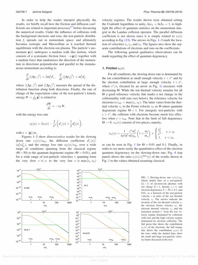
range of conditions spanning from the classical regime(H! 50) to the quantum degenerate regime (H ! 0:01), andfor a wide range of test-particle velocities v spanning formthe very slow v. vi to the very fast v/ max"ve; vF#

velocity regimes. The results shown were obtained settingthe Coulomb logarithms to unity, lnkte ! lnKti ! 1, to high-light the effect of quantum statistics on the momentum inte-gral in the Landau collision operator. The parallel diffusioncoefficient is not shown since it is simply related to "t"v#according to Eq. (13). The arrows in Figs. 1–3 mark the loca-tion of velocities vi, ve, and vF. The figures also show the sep-arate contributions of electrons and ions on the coefficients.

The following general qualitative observations can bemade regarding the effect of quantum degeneracy.

1. Friction mt "v#

For all conditions, the slowing down rate is dominated bythe ion contzribution at small enough velocity v < v? and bythe electron contribution at large enough velocity v > v?,where v?=vi (located by an arrow in Fig. 1) increases withdecreasing H. While the ion thermal velocity remains for allH a good reference velocity that marks a net change in thecollisionality with ions (see below), the reference velocity forelectrons is vref ! max"ve; vF#. The latter varies from the ther-mal velocity ve to the Fermi velocity vF as H enters quantumdegenerate regime H < 1. For energetic test-particles withv > v?, the collision with electrons become much less effec-tive when v > vref . Note that in the limit of full degeneracyH! 0; "te"v# consists of two pieces, namely,

"te v" # !1

3p2"h3

ctem3e

m2t lte

1$ mt

me

- .(

v3F

v3; v > vF

1; v < vF;

8<

:

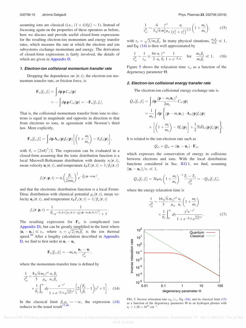
as can be seen in Fig. 1 for H ! 0:01 and 0.1. Finally, inorder to see more easily the quantitative effect of the electronquantum degeneracy on the slowing-down rate, Fig. 4 (toppanel) shows the ratio "t"v#="class

t "v# of the results shown inFig. 1 to the values obtained assuming classical.

FIG. 1. Slowing-down rate "t"v#=xpe

(black dotted line) of a test-particle(Zt! 1) of electron-ion plasmas withion charge Zi! 1, density rs! 1, andelectron degeneracy h ! 50; 1; 0:1, and0.01, as a function of the test-particlevelocity v in units of the ion thermalvelocity vi. The arrows indicate thelocation of the ion thermal velocity vi,the electron Fermi velocity vF, theelectron thermal velocity ve, and thetransition around v? from the low ve-locity regime dominated by collisionswith ions and the high velocity regimedominated by electron collisions. Thefull green line shows the contribution"te"v# of the electrons, the full orangeline shows the contribution "ti"v# ofthe ions, while the dashed lines showthe small and large test-particle veloc-ity limits discussed in the text.



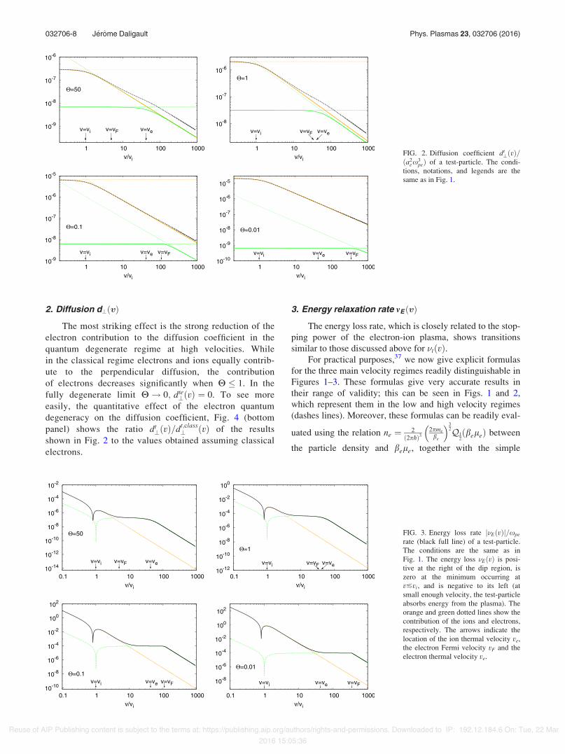
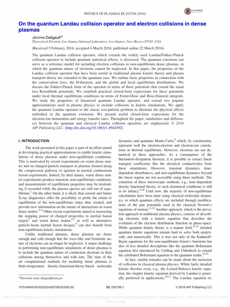
2. Diffusion d?"v#

The most striking effect is the strong reduction of theelectron contribution to the diffusion coefficient in thequantum degenerate regime at high velocities. Whilein the classical regime electrons and ions equally contrib-ute to the perpendicular diffusion, the contributionof electrons decreases significantly when H 0 1. In thefully degenerate limit H! 0; dte

?"v# ! 0. To see moreeasily, the quantitative effect of the electron quantumdegeneracy on the diffusion coefficient, Fig. 4 (bottompanel) shows the ratio dt

?"v#=dt;class? "v# of the results

shown in Fig. 2 to the values obtained assuming classicalelectrons.

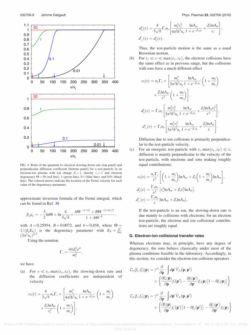
3. Energy relaxation rate mE "v#

The energy loss rate, which is closely related to the stop-ping power of the electron-ion plasma, shows transitionssimilar to those discussed above for "t"v#.

For practical purposes,37 we now give explicit formulasfor the three main velocity regimes readily distinguishable inFigures 1–3. These formulas give very accurate results intheir range of validity; this can be seen in Figs. 1 and 2,which represent them in the low and high velocity regimes(dashes lines). Moreover, these formulas can be readily eval-

uated using the relation ne ! 2"2p"h#3

2pmebe

( )32Q1

2"bele# between

the particle density and bele, together with the simple

FIG. 2. Diffusion coefficient dt?"v#=

"a2ex

3pe# of a test-particle. The condi-

tions, notations, and legends are thesame as in Fig. 1.

FIG. 3. Energy loss rate j"E"v#j=xpe

rate (black full line) of a test-particle.The conditions are the same as inFig. 1. The energy loss "E"v# is posi-tive at the right of the dip region, iszero at the minimum occurring atv!vi, and is negative to its left (atsmall enough velocity, the test-particleabsorbs energy from the plasma). Theorange and green dotted lines show thecontribution of the ions and electrons,respectively. The arrows indicate thelocation of the ion thermal velocity ve,the electron Fermi velocity vF and theelectron thermal velocity ve.



approximate inversion formula of the Fermi integral, whichcan be found in Ref. 38

bele ! )3

2lnH$ ln

4

3,,,pp $ AH) 1$b" # $ BH) 1$b" #=2

1$ AH)b ;

with A! 0.25954, B! 0.0072, and b! 0.858, where H !1="beEF# is the degeneracy parameter with EF ! "h2

2me

"3p2ne#2=3.Using the notation

Ct !4pZ2

t e4

m2t

;

we have

(a) For v. vi;max"ve; vF#, the slowing-down rate andthe diffusion coefficients are independent ofvelocity

"t v" # !4

3,,,pp neCt (

m3e

4p32"h3ne

lnKte

1$ e)bele1$ mt

me

- ."

$ ZilnKti

v3i

1$ mt

mi

- .#

;

dtk v" # !

4

3,,,pp Ctne

m3ev

2e

4p32"h3ne

lnKte

1$ e)bele$ ZilnKti

vi

" #

;

dt?"v# ! dt

k"v#:

Thus, the test-particle motion is the same as a usualBrownian motion.

(b) For vi . v. max"ve; vF#, the electron collisions havethe same effect as in previous range, but the collisionswith ions have a much different effect

"t v" # ! neCt (m3

e

3p2"h3ne

lnKte

1$ e)bele1$ mt

me

- ."

$ ZilnKti

v31$ mt

mi

- .#

;

dtk v" # ! Ctne

m3ev

2e

3p2"h3ne

lnKte

1$ e)bele$ ZilnKtiv2

i

v3

" #

;

dt? v" # ! Ctne

m3ev

2e

3p2"h3ne

lnKte

1$ e)bele$ ZilnKti

v

" #

:

Diffusion due to ion collisions is primarily perpendicu-lar to the test-particle velocity.

(c) For an energetic test-particle with vi;max"ve; vF# . v,diffusion is mainly perpendicular to the velocity of thetest-particle, with electrons and ions making roughlyequal contributions:

"t v" # !neCt

v31$ mt

me

- .lnKte $ Zi 1$ mt

mi

- .lnKti

" #;

dtk v" # !

Ctne

v3v2

e lnKte $ Ziv2i lnKti

# $;

dt? v" # !

Ctne

vlnKte $ ZilnKti& ':

If the test-particle is an ion, the slowing-down rate isdue mainly to collisions with electrons; for an electrontest-particle, the electron and ion collisional contribu-tions are roughly equal.

G. Electron-ion collisional transfer rates

Whereas electrons may, in principle, have any degree ofdegeneracy, the ions behave classically under most of theplasma conditions feasible in the laboratory. Accordingly, inthis section, we consider the electron-ion collision operators

Cei fe; fi& ' p" # ! cei @

@p%"

dp0 V$

ei p; p0* +

(@fe p" #@p

fi p0* +) @fi p0" #

@p0fe p" # 1) hfe p" #

# $/ 0

Cie fi; fe& ' p" # ! cei @

@p%"

dp0 V$

ie p; p0* +

(@fi p" #@p

fe p0* +

1) hfe p0* +# $

) @fe p0" #@p0

fi p" #/ 0

FIG. 4. Ratio of the quantum to classical slowing-down rate (top panel) andperpendicular diffusion coefficient (bottom panel) for a test-particle in anelectron-ion plasma with ion charge Zi! 1, density rs! 1 and electrondegeneracy H! 50 (red line), 1 (green line), 0.1 (blue line), and 0.01 (blackline). The colored arrows indicate the location of the Fermi velocity for eachvalue of the degeneracy parameter.



assuming ions are classical (i.e., "1$ dihifi# , 1). Instead offocussing again on the properties of these operators as before,here we discuss and provide useful closed-form expressionsfor the resulting electron-ion momentum and energy transferrates, which measure the rate at which the electron and ionsubsystems exchange momentum and energy. The derivationof closed-form expressions is fairly involved, the details ofwhich are given in Appendix D.

1. Electron-ion collisional momentum transfer rate

Dropping the dependence on "r; t#, the electron-ion mo-mentum transfer rate, or friction force, is

Fei&fe; fi' !"

dp p Cei"p#

! )"

dp p Cie"p# ! )Fie&fi; fe':

That is, the collisional momentum transfer from ions to elec-trons is equal in magnitude and opposite in direction to thatfrom electrons to ions, in agreement with Newton’s thirdlaw. More explicitly,

Fei fe; fi& ' !"

dp Aei p" #fe p" # 1$ mi

me

- .) hefe p" #

% &;

with he ! "2p"h#3=2. The expression can be evaluated in aclosed-form assuming that the ionic distribution function is alocal Maxwell-Boltzmann distribution with density ni"r; t#,mean velocity ui"r; t#, and temperature kBTi"r; t# ! 1=bi"r; t#

fi r; p; t" # ! nibi

2pmi

- .32

e)bi

2mip)miui" #2 ;

and that the electronic distribution function is a local Fermi-Dirac distribution with chemical potential le"r; t#, mean ve-locity ue"r; t#, and temperature kBTe"r; t# ! 1=be"r; t#

fe r; p; t" # !1

he

1

e)be r;t" # le r;t" #) 12me

p)meue r;t" #" #2& ' $ 1:

The resulting expression for Fei is complicated (seeAppendix D), but can be greatly simplified in the limit wherejui ) uej. vi, where vi !

,,,,,,,,,,,,,,2=mibi

pis the ion thermal

speed.39 After a lengthy calculation described in AppendixD, we find to first order in ui ) ue

Fei fe; fi& ' ! )meneue ) ui

sFei

;

where the momentum-transfer time is defined by

1

sFei

! 8,,,pp

3

mecei

lei

ni

ne

bi

be

( 1

he

"1

0

dye)y2

1$ e)bele emebemibi

y22

be

bi) 1

- .y2$ 1

% &: (14)

In the classical limit bele ! )1, the expression (14)reduces to the usual result17,40

1

sFei

, 4

3,,,pp cei

m2elei

ni

v2e $ v2

i

* +3=21$ me

mi

- .; (15)

with ve !,,,,,,,,,,,,,,,2=mebe

p. In many physical situations, mebe

mibi. 1,

and Eq. (14) is then well approximated by

1

sFei

, 1

sei- 4p

3

ni

ne

cei

he

1

1$ e)belefor

mebe

mibi. 1: (16)

Figure 5 shows the relaxation time sei as a function of thedegeneracy parameter H.

2. Electron-ion collisional energy transfer rate

The electron-ion collisional energy exchange rate is

Qei fe; fi& ' !"

dpp) meue" #2

2meCei p" #

! 1

me

"dp

(

p) meue" # % Aei p" #fe p" #

( 1$ mi

me

- .) hfe p" #

% &$ 1

2TrD

$

ei p" #fe p" #

)

:

It is related to the ion-electron rate such as

Qei $ Qie ! "ui ) ue# % Fei;

which expresses the conservation of energy in collisionsbetween electrons and ions. With the local distributionfunctions considered in Sec. II G 1, we find, assumingjjui ) uejj=vi . 1,

Qei fe; fi& ' ! 3kBne 1$ mi

me

- .)1 Ti ) Te

sQei

! )Qie fi; fe& ';

where the energy relaxation time is

1

sQei

! 16,,,pp

3

mecei

lei

ni

ne1$ me

mi

- .

( 1

he

"1

0

dyy2e)y2

1$ e)bele emebemibi

y2: (17)

FIG. 5. Inverse relaxation rate xpe=sei, Eq. (16), and its classical limit (15)as a function of the degeneracy parameter H in an hydrogen plasma withne ! 1:28( 1025 cm)3.



In the classical limit bele ! )1, the expression (17)reduces to the usual result17

1

sQei

, 4

3,,,pp cei

m2elei

ni

v2e $ v2

i

* +3=21$ me

mi

- .:

In the limit mebemibi. 1, Eq. (17) is well approximated by

1

sQei

, 1

sei;

where sei is defined as in Eq. (16). This result corresponds tothe popular result of Brysk et al.30 that was obtained byextending the usual binary Coulomb collision calculation ofSpitzer40 to include the Pauli principle. Further discussion onsei in dense plasmas can be found in Ref. 41.

III. LINEARIZED QUANTUM LANDAU COLLISIONOPERATOR: ELECTRON-ELECTRON COLLISIONS

The non-linearity of a collision operator is essential if thestate of the system is far from local thermal equilibrium.However, in the important situations where the phase-spacedistribution f remains near local thermal equilibrium f0, thelinearized form of the collision operator provides an accuratedescription of the dynamics of the deviation df ! f ) f0,while the dynamics of f0 is governed the hydrodynamic equa-tions through its dependence on the thermodynamic variables.More generally, linearized collision operators play an impor-tant role in the mathematical analysis of kinetic equationsbased on perturbation expansions, such as in the celebratedChapman-Enskog method. Moreover, linearized collisionoperators are at the basis of advanced numerical algorithms toinclude the effect of collisions in kinetic simulations (e.g., thedf-method in traditional plasma physics21,42,43). The extensionof such algorithms to the qLFP operator could be used in theapplications to dense plasmas briefly mentioned in Sec. II. Inthis section, we discuss the properties of the operator obtainedby linearizing the qLFP operator around local equilibrium.First we describe general properties in connection with theconservation laws, the stationary states, and the self-adjointness and positivity of the linerarized operator. Fromthese properties, the well-known Chapman-Enskog solutionof the classical Boltzmann equation20 can be straightfor-wardly adapted to the qLFP operator. Then we discuss twoapproximations of the linearized qLFP operator that can beuseful in numerical implementations of the latter for modelingdense plasmas near local equilibrium.

We focus on the linearization of the operator Caa for like-particle collisions; the extension to unlike-particle collisionoperator Cab is straightforward. For definiteness, but withoutlack of generality, we consider the electron-electron collisionoperator (setting da ! )1, ga! 2 in the Caa). For simplicityof notation, we drop the subscript “e” in most expressions.

A. Generalities

We assume that at every space-time position "r; t#, themomentum distribution function can be decomposed as

f ! f0 $ df ;

where

f0 r; p; t" # !2

2p"h" #31

e)b r;t" # l r;t" #) 12m p)mu r;t" #" #2& ' $ 1

is the local Fermi-Dirac distribution function and

df . f :

For convenience we define the momentum in the referenceframe

g"r; p; t# ! p) mu"r; t#; g ! jgj;

and the function F0"g# ! f0"g$ mu#.Expanding the electron-electron qLFP collision operator

to first order in df , we obtain

Cee&f ; f ' ! Cee&f0; f0'|11111{z11111}!0

$ Cdf $ O"df 2#;

where

Cdf ! C1&f0; df ' $ C2&df ; f0'

is the linearized qLFP collision operator.

1. First term

C1 is a differential operator acting on df , more preciselya linear Fokker-Planck operator

C1 f0; df& ' ! ) @

@p% C df ) 1

2

@

@p% D

$df

( )% &; (18)

where the friction vector C and diffusion tensor D$

are inde-pendent of df and are given by

C ! "1) 2hf0#Aee&f0' $ Bee&f0'; (19)

D$! D

$

ee&f0' (20)

in terms of the friction vectors and diffusion tensor definedin Eq. (9). Using the expressions (12) for the potentials inlocal equilibrium into Eq. (9), we obtain the followingclosed-form expression:

C"r; p; t# ! c"r; g; t#g;

D$

r; p; t" # ! dk r; g; t" #gg

g2$ d? r; g; t" # I

$) gg

g2

- .;

where

c"g# ! a"g#"1) 2hF0"g## $ b"g#

and

a g" # ! )4cee

g3

m

2p"h2b

- .32

Q12

bl; x" #; (21a)



b g" # ! )4cee

g3

m

2p"h2b

- .32

Q)12

bl; x" # $ 8pceem

bg2F0 g" #;

dk g" # ! )2m

ba g" #; (21b)

d? g" # !4cee

g

m

2p"h2b

- .32

Q)12

bl; x" # ) 1

2dk g" #; (21c)

where x ! b2m g2.

In the classical limit, C1 reduces to the collision(Fokker-Planck) operator of a test-particle colliding with aMaxwellian background.17 In contrast, the general expres-sion (18) differs from that of a test-particle moving in theequilibrium, Fermi-Dirac electronic background (as previ-ously discussed in Sec. II E). Nevertheless, C1 can still beregarded as a drag-diffusion operator in momentum space,with drag coefficient c and diffusion coefficients dk and d?.

2. Second term

The second term

C2 df ; f0& ' ! ) @

@p% dC df& 'f0 )

1

2

@

@p% dD

$df& 'f0

h i/ 0;

where

dC&df ' ! "1) hf0#Aee&df ' $ Bee&"1) 2hf0#df ';

dD$&df ' ! D

$

ee&"1) 2hf0#df ':

The term C2 consists of source and sink terms that enforcethe conservation laws of the full operator C . While simplerthan the non-linear operator Cee; C2 is nevertheless still com-plicated to deal with analytically and numerically since it isa non-local integral operator of the form

C2&df ; f0'"p# !"

dp0K"p; p0#df "p0#: (22)

Below we discuss approximations of C2 that can be used tofacilitate its treatment in practical applications.

3. Alternative expression

For some applications, the following expression of thelinearized operator C can be useful

Cdf ! cee @

@p%"

dp0 V$

p; p0* +

%@/ p" #@p

) @/ p0" #@p0

% &:

where df ! f0"1) hf0#/.

B. Properties

The linearized operator C has most of the same proper-ties as the non-linear collision term Cee (see Sec. II C) and asits classical counterpart.17 The properties listed here can beimportant in analytical works and numerical applications.Interestingly, several of them are satisfied separately by theterms C1 and C2.

1. Collisional invariants

The quantities "1; p; p2# are the collisional invariants ofC, i.e.,

"dp wCdf ! 0 for w ! 1; px; py; pz; p

2:

2. Self-adjointness

This important property of the linearized collision oper-ator is arguably more difficult to prove than in the classicalcase. The details of the proof are given in Appendix E 1.

Let df ! f0"1) hf0#a, where a is a scalar function ofmomentum p; we define

I0"a# ! Cdf ! I1"a# $ I2"a#;

with

I1"a# ! C1&f0; df '; I2"a# ! C2&df ; f0':

Given two functions a and b of the momentum p, we definethe bracket integrals

&a; b'n !"

dp bIn"a# with n ! 0; 1; 2:

The following properties are satisfied:

(a) the bracket integrals are bilinear, symmetric forms, i.e.,

&a; b'n ! &b; a'n with n ! 0; 1; 2: (23)

(b) I0 is a semi-definite positive operator in the sense that,for arbitrary a

&a; a'0 + 0:

The equality sign holds if and only if a is a linear com-bination of the collisional invariants

a"p# ! c0 $ c1 % p$ c2p2; (24)

where c0, c1, and c2 are independent of p;(c) consequently, the general solution of the homogeneous

integral equation I0"a# ! 0 is given by Eq. (24), i.e.,

Cdf ! 0 () df ! "c0 $ c1 % p$ c2p2#f0"1) hf0#:(25)

Physically, Eq. (25) can be regarded as the generalexpression for the modification of a local Fermi-Diracdistribution function due to perturbations in the ther-modynamic variables l, b, and u, Taylor expanded tofirst order in these perturbation. Indeed, by substitutingl$ dl for l (and similarly for b and u) in Eq. (18),and Taylor expanding with respect to the variationsdl; db and du, the first order term is

df ! bdl$ l)p) mu" #2

2m

- .db$ b p) mu" # % du

% &

( f0 1) hf0" #:



C. Approximations

As mentioned above, in applications, rather than use thecomplicated integral operator C2, it may be more convenientto employ a simpler approximate operator that shares asmany properties as possible with the exact operator. At theleast, to be physically acceptable, one should replace C2 by aterm that guarantees local particle number, momentum, andenergy conservation such that the particles, momentum, andenergy removed by the drag-diffusion term C1 is replenishedby the approximate C2.

In the following, we generalize two approximations of theclassical, linearized Fokker-Planck operator commonly used intraditional plasma physics.42–45 We begin by extending to thequantum case the approximation introduced by Catto andTsang and later by other authors,42,44,45 and then we considerthe refined formulation of Lin, Tang, and Lee.43 For conven-ience, we remark that both approximations can be written as

C2&df ; f0' * f0"1) hf0#O&df ';

with

O&df ' ! )K %"

dp0 &p0 ) mu'C1&f0; df 0'

)E"

dp0 &a"p0 ) mu#2 $ b'C1&f0; df 0' (26a)

! )K %"

dp0 Cdf 0

)E"

dp0 a&2C % "p0 ) mu# $ TrD$'df 0; (26b)

where df 0 ! df "r; p0; t# (note that in deriving the last equa-tion (26b), b was assumed to be independent of p0).

Comparing Eqs. (26) with (22), one sees that the formeris significantly simpler to evaluate for different values of themomentum p than the exact operator; in particular, the mo-mentum integrals of df in O&df '"r; p; t# is the same for allvalues of p and, in contrast to Eq. (22), need to be evaluatedonly once at each space-time point "r; t#.

1. First approximation

Although not explicitly mentioned in the original papers,the approximation of Refs. 44 and 45 is obtained by expandingthe classical limit C2&df ; f0' over orthogonal trivariate polyno-mials with respect to the local Maxwellian distribution func-tion, e.g., the Hermite tensor polynomials introduced byGrad,46 and then keeping only the terms that are strictly neces-sary to ensure the conservation of particle number, momentum,and energy, and setting all the other terms to zero. The general-ization to the quantum case requires polynomials orthogonalwith respect to f0"1) hf0#, which leads to Eq. (26) with

a ! bm; b ! )3

Q12

bl" #Q)1

2bl" #

:

One can easily verify47,48 that the polynomials H"g# ! 1,gi (i! 1, 2, 3), and ag2 $ b are, indeed, orthogonal with respectto f0"1) hf0#. Enforcing the constraints of conservation of

particle number, momentum and energy, we obtain the follow-ing expressions for K and E:

K"r; p; t# ! aK"r; t#g;

with

aK !1

3

"dp g2f0 1) hf0" #

% &)1

! nmkBTQ1

2bl" #

Q)12

bl" #

" #)1

and

E r; p; t" # ! aE r; t" # b"p) mu r; t" ##2

m) 3Q1

2bl" #

Q)12

bl" #

!;

with

aE !"

dpbm

g2 ) 3Q1

2bl" #

Q)12

bl" #

!2

f0 1) hf0" #

2

4

3

5)1

! 15nQ3

2bl" #

Q)12

bl" #) 9n

Q12

bl" #Q)1

2bl" #

!22

4

3

5)1

:

In the classical limit bl! )1 obtained using Q""t# , 1for t! )1, the previous expressions give

aK !1

mnkBT; aE !

1

6n;

which correspond to the usual values used in theliterature.44,45

2. Second approximation

This approximation improves the first approximation inthat, like the exact operator, it annihilates functions df of theform (25). The approximation corresponds to setting

a ! 1; b ! 0;

in Eq. (26) together with

K"r; p; t# ! aK"r; t#C"r; p; t# ! aK"r; t#c"r; g; t#g;

with

aK !1

3

"dp cg2f0 1) hf0" #

% &)1

! 4cee

3h2

2pm

b

- .52

Q)32

bl" # )Q)12

bl" #( )

" #)1

(27)

and

E"r; p; t# ! aE"r; t#&2C"r; p; t# % g$ TrD$"r; p; t#'

! aE"r; t#&2c"r; g; t#g2 $ dk"r; g; t# $ 2d?"r; g; t#';

with



aE !"

dp 2cg4 $ dk $ 2d?* +

g2h i

f0 1) hf0" #% &)1

! 128 p5=2cee

h2

m

b

- .72

Q)12

bl" # )Q12

bl" #( )

" #)1

:

In the classical limit (obtained using the series expansionF ""t# ! z) z2

2"$1 $ o"z2# with z ! et), the previous expres-sions give

aK ! ) 2n2cee

3

,,,,,,,b

mp

r !)1

; aE ! )4n2cee

,,,,,,m

pb

r !)1

;

which correspond to those originally proposed by Linet al.21,43

This approximation satisfies many properties of theexact operator previously discussed in Sec. III B.

3. Self-adjointness

Let df ! f0"1) hf0#a, and

I~2&a' - f0"1) hf0#Odf ; &a; b'~2!"

dp bI~2&a':

Then, by construction, as shown in Appendix E 2

&a; b'~2! &b; a'~2 : (28)

As a consequence, the approximate linearized collisionoperator

~Cdf ! C1"f0; df # $ f0"1) hf0#O&df '

is also self-adjoint.

4. Conservation laws

By construction, the quantities "1; p; p2# are the collisioninvariants of ~C, i.e.,

"dp"c0 $ c1 % p$ c2p2#~Cdf ! 0; 8df ; (29)

where c0, c1, and c2 are independent of p.

5. Stationary states

~C satisfies49

~Cdf ! 0 () df ! "c0 $ c1 % p$ c2p2#f0"1) hf0#:

Like the exact linearized operator C (see Eq. (25), butunlike the first approximation, the second approximationannihilates the collisional steady states, i.e., the linearlyshifted Fermi-Dirac distribution functions. This is becauseby taking into account the momentum dependence of themomentum and energy exchange rates induced by colli-sions, the second approximation maintains a linearly shiftedFermi-Dirac distribution by restoring the momentum andenergy according to their loss rates. In contrast, in the firstapproximation, an initially linearly shifted Fermi-Dirac dis-tribution function is being distorted in momentum spaceover time.

IV. CONCLUSION

We have extended many of the standard properties ofthe classical Landau-Fokker-Plank collision operator widelyused in plasma physics to the quantum Landau collision op-erator, which extends the former operator to include effectsof quantum statistics. First, we have discussed generalaspects of the qLFP operator, including properties in connec-tion with the conservation laws, the H-theorem, and theglobal and local equilibrium distributions; its Fokker-Planckform in terms of three potentials that extend the usual twoRosenbluth potentials; the establishment of useful closed-form expressions for these potentials in terms of Fermi-Diracand Bose-Einstein integrals; the application of the latter tothe classic test-particle problem to illustrate the physicsembodied by the qLFP operator; the development of usefulclosed-form expressions for the electron-ion momentum andenergy transfer rates. Then, we have discussed the basicproperties of the linearized qLFP operator, and extended twoclassic approximations of its classical counterpart that can beuseful in numerical implementations. The algebraic manipu-lations needed in establishing useful, closed-form expres-sions are arguably less straightforward than in the classicalcase. We have therefore given all the derivations in theappendixes not only for completeness but also because the“tricks” used could potentially be useful to other quantum ki-netic theory calculations.

ACKNOWLEDGMENTS

This work was performed under the auspices of theUnited States Department of Energy under Contract No. DE-AC52-06NA25396. This research was supported by the DOEOffice of Fusion Energy Sciences, and by an LDRD grant atLos Alamos National Laboratory.

APPENDIX A: A DERIVATION OF THE QUANTUMLANDAU COLLISION OPERATOR

We present a physicist’s derivation of the qLFP colli-sion operator. For simplicity of notation, we consider anelectron plasma in a uniform positive charge background;in this appendix, m is the electron mass, u"k# ! 4pe2=k2 isFourier transform of the bare Coulomb potential energye2=r of two electrons at a distance r apart. We startfrom the quantum Boltzmann (qB) collision integral forthe rate of change of the number of electrons in momen-tum state p

CqB f ; f& ' p" # !"

dp0"

dq

2p"h" #3v q="h" #

! q="h;q % p"hm$ q2

2m

- .

''''''''

''''''''

2

( 2pm

"hd q % p) p0 $ q

* +* +

( fp$qfp0)q 1) hfp* +

1) hfp0* +#

) fpfp0 1) hfp$q* +

1) hfp0)q* +

' ; (A1)



where the transition probability per unit time for Coulomb scattering of two electrons from momentum state p; p0 to momen-tum states p$ q; p) q accounts for the screening effect via the dielectric function !"k;x#.29

The qLFP collision integral is obtained by retaining in CqB only the small angle scattering events. This is done by expand-ing the integrand in powers of the momentum transfer q and keeping only the leading term. While the calculation does notpresent any major difficulty, the bookkeeping of terms of the same order requires some attention in order to reduce to the com-pact form Eq. (3). Below we outline the main steps.

We combine the expansion to first-order in q of both the delta function

d q % p) p0 $ q* +* +

* d q % p) p0* +* +

$ q % @@p

d q % p) p0* +* +

and the dielectric function

v q="h" #

! q="h;q % p"hm$ q2

2m

- .

''''''''

''''''''

2

* v q="h" #

! q="h;q % p"hm

- .

''''''''

''''''''

2

$ q

2% @@p

v q="h" #

! q="h;q % p"hm

- .

''''''''

''''''''

2

;

with the Taylor expansion to second order in q of the term in brackets in Eq. (A1)

:::& ' * q %@fp@p

fp0 1) hfp0* +

) q %@fp0

@p01) hfp* +

fp

% &$ 1

2q % Dfp % qfp0 1) hfp0

* +$ 1

2q % Dfp0 % qfp 1) hfp

* +%

) q % @fp@p

- .q % @fp0

@p0

- .1) hfp* +

1) hfp0* +&

: (A2)

The term of first order vanishes upon integration over q and the terms of second order is

v q="h" #

! q="h;q % p"hm$ q2

2m

- .

''''''''

''''''''

2

d q % p) p0 $ q* +* +

fp$qfp0)q 1) hfp* +

1) hfp0* +

) fpfp0 1) hfp$q* +

1) hfp0)q* +# $

* 1

2

v q="h" #

! q="h;q % p"hm

- .

''''''''

''''''''

2

@

@p) @

@p0

- .% q d q % p) p0

* +* +q %

@fp@p

fp0 1) hfp0* +

)@fp0

@p0fp 1) hfp* +% &/ 0

$ q

2% @@p

v q="h" #

! q="h;q % p"hm

- .

''''''''

''''''''

2

( d q % p) p0* +* +

q %@fp@p

fp0 1) hfp0* +

) q %@fp0

@p01) hfp* +

fp

% &:

Hence, to lowest order in q, we find

CqB f ; f& ' p" # * mp@

@p%"

dp0"

dk

2p" #3v k" #

! k;k % p

m

- .

''''''''

''''''''

2

( d k % p) p0* +* +

kk %@fp

@pfp0 1) hfp0* +

)@fp0

@p0fp 1) hfp* +% &

: (A3)

Equation (A3) can be regarded as the quantum extension of the classical Lenard-Balescu collision integral (in the literature,Eq. (A1) is often abusively referred to as the quantum Lenard-Balescu equation15). Like in the classical case, the qLFP equa-tion is obtained in the static limit !"k; k%p

m #! !"k; 0#, leading to

CqLFP f ; f& ' p" # !m

8p2

@

@p%"

dp0 G$

p) p0* +

%@fp@p

fp0 1) hfp0* +

)@fp0

@p0fp 1) hfp* +% &

where

G$

g" # !"

dkv k" #! k; 0" #

''''

''''2

d k % g" #kk ! p 4pq2* +2

lnKg2 I$) gg

g3;



with g ! p) p0, and

lnK !"1

0

dk

k

'''1

! k; 0" #

'''2

(A4)

is the Coulomb logarithm.

APPENDIX B: IMPORTANT PROPERTIES OF THEFERMI-DIRAC FUNCTION

The quantum equilibrium distribution function

fq p; b; l" # ! 1

h1

e)b l)p2

2m

* +) d

satisfies

1

b@

@lfq ! fq 1$ dhfq" #

1

b2

@2

@l2fq ! fq 1$ dhfq" # 1$ 2dhfq" #

@

@pfq ! )

bm

pfq 1$ dhfq" #:

(B1)

We emphasize these properties because the fact that productsof the form fq"1$ dhfq# and fq"1$ dhfq#"1$ 2dhfq# can besimply expressed in term of derivatives of f is essential inderiving the most of the results of the main text. This prop-erty of the equilibrium quantum distribution function is quitefortunate. In the classical case, the equivalent properties sat-isfied by the Maxwell-Boltzmann distribution (more pre-cisely of the underlying exponential function) are evensimpler and are often unnoticed, but they are similarly essen-tial to our ability to write closed-form formulas.

In addition, the majority of the closed-form results wereobtained by noticing the following relation between thequantum distribution function and the Maxwell-Boltzmanndistribution function

fq p; b; l" # ! 2pm" #3=2

n

1

h

"1

)1dE

1

e)b l)E" # ) d

("i1

)i1

dz

2pi

ezE

z3=2fcl p; z" # ; (B2)

where

fcl p; b" # ! nb

2pm

- .3=2

e)b

2mp2

:

Equation (B2) simply follows from 11$ea)x2 !

!$1)1

1ea)y)d

d"y) x2# and d"y) x2# !!1)1

dt2p eit"y)x2# !

! i1)i1

dz2pi ezye)zx2

!! i1)i1

dz2pi

ezy

z3=2 z3=2e)zx2. The relation (B2) provides a link

between the classical results and the quantum results.Indeed, the classical expression for the Rosenbluth potentialsand related quantities is momentum integrals of the form

Icl"b# !"

dv Q"v#~fcl"v; b#;

while their quantum counterparts (10) are of the form

Iq"b; l# !"

dv Q"v#~fq"v; b; l#;

and

Jq b; l" # !"

dv Q v" #~fq v; b" # 1$ d~h~fq v; b; l" #( )

! 1

b@

@lIq b; l" # ; (B3)

where we used Eq. (B1) in the last expression. KnowingIcl"b#, Iq, and Jq can be obtained using

Iq b; l" # ! 2pm" #3=2

n

1

h

"1

)1dE

1

e)b l)E" # ) d

("i1

)i1

dz

2pi

ezE

z3=2Icl z" # ; (B4)

which results from the relation (B2). This way the quantumcalculation amounts first to an integral in the complexplanes, which, for the cases of interest here, can be doneusing Cauchy’s residues theorem. The remaining integralover E yields to Fermi integrals.

APPENDIX C: CALCULATION OF POTENTIALS H, I,AND G IN LOCAL THERMAL EQUILIBRIUM

All closed-form expressions for the potentials H, I, and Gare obtained by applying the method outlined in Appendix B.

1. Potential H

We have

H v" # !"

dv01

jjv) v0jjfq v0; b" #

! 2pm" #3=2

n

1

h

"1

)1dE

1

e)b l)E" # ) d

("i1

)i1

dz

2pi

ezE

z3=2Hcl v; z" # ;

where

Hcl v; b" # !"

dv01

jjv) v0jj~fcl v0; b" # ! n

verf

,,,,,,,mb2

rv

!

is the classical Rosenbluth potential. The complex integral isperformed as follows:

"i1

)i1

dz

2pi

ezE

z3=2Hcl v; z" # !

,,,,,,2mp

n,,,pp

v

"i1

)i1

dz

2pi

ezE

z

"v

0

e)mz2 x2

dx

!,,,,,,2mp

n,,,pp

v

"v

0

dx

"i1

)i1

dz

2pi

ez E)mx2=2" #

z

!,,,,,,2mp

n,,,pp

v

"v

0

dx H E) mx2=2* +

;



where we used"a$i1

a)i1

dz

2pi

ezx

z! H x" #: (C1)

Therefore,

H v" # !4pm

v1

h

"v

0

dx

"1

mx2=2

dE1

e)b l)E" # ) d

! 4pm2

bhQc

0 bl;mbv2

2

- .

$ 1

vh2pm

b

- .3=2

Q1=2 bl;mbv2

2

- .; (C2)

after an integration by parts.

2. Potential I

The potential I is obtained by applying Eq. (B3) to (C2),i.e.,

I v" # !"

dv01

jjv) v0jj~fq v0;b" # 1$ d~h~fq v0;b" #

( )! 1

b@

@lH v" #:

3. Potential G

We again apply Eqs. (B3) and (B4), i.e.,

G v" # !"

dvjv) v0j~fq v0" # 1$ d~h~fq v" #h i

! 1

b@

@lg v" #;

where

g"v# !"

dv0jjv) v0jj~fq"v0; b# (C3)

! 2pm" #3=2

n

1

h

"1

)1dE

1

e)b l)E" # ) d

("i1

)i1

dz

2pi

ezE

z3=2gcl v; z" # ; (C4)

and gcl is the classical Rosenbluth potential

gcl v; b" # !"

dv0jjv) v0jj ~fcl v0; b" #

! n v$ 1

mbv

- .erf

,,,,,,,mb2

rv

!

$

,,,,,,,,,2

pmb

s

e)mb2 v2

2

4

3

5:

The complex integral is"i1

)i1

dz

2pi

ezE

z3=2gcl v; z" #

! n

"i1

)i1

dz

2pi

ezE

z3=2( v$ 1

mvz

- . ,,,,,,,,2mz

p

r "v

0

e)mb2 x2

dx

"

$,,,,,,,,

2

pmz

re)

mz2 v2

#

!,,,,,,2m

p

rnv"i1

)i1

dz

2pi

ezE

z

"v

0

e)mb2 x2

dx$,,,,,,,2

mp

rn

v

"i1

)i1

dz

2pi

ezE

z2

"v

0

e)mb2 x2

dx$,,,,,,,2

pm

rn

"i1

)i1

dz

2pi

ezE

z2e)zmv2

2 :

Using! a$i1a)i1

dz2pi

ezx

z2 ! )xH"x# and Eq. (C1), we then find

g v" # ! v2H v" # $4pv

1

h

"v

0

dx

"1

0

E

1$ e)b l)mx2

2 )E" #

$4pm1

h

"1

0

E

1$ e)b l)mp2

2 )E* + :

Using!1

0 dE 1

1$e)b"l)mx22)E#! ln 1$ eb"l)mx2

2 #( )

and Eq. (B1),we find

G v" # ! v2I v" # $1

b2pm

b

- .3=2 1

vQ1=2 bl;

mb2

v2

- .

$ 8pm

b2

1

hln 1$ eb l)mv2

2

* +( );

where we used an integration by parts.

APPENDIX D: FORMULAS FOR Rei AND Qei

1. Friction force Rei

We again apply the method outlined in Appendix B to

Fei !"

dppCei fq& ' p" #

!"

dpAei p" #fq p" # 1$ mi

me

- .) hefq p" #

% &

! mi

mefei $

1

be

@

@lefei; (D1)

where

fei -"

dpAei p" #fq p" #

! 2pme" #3=2

ne

1

he

"1

)1dE

1

1$ e)be le)E" #

("i1

)i1

dz

2pi

ezE

z3=2fcl

ei z" # (D2)

and

fclei -

"dpAei"p#fcl"p#:

In the following, we first determine fclei and substitute the

result into Eqs. (D2) and (D1).

a. Evaluation of fclei

We will first show that

fclei !

ceineni

milei

@

@u

1

uerf

u

v2i $ v2

e

* +1=2

!" #(D3)

*) cei

milei

4nine

3,,,pp 1

v2e $ v2

i

* +3=2ue ) ui" # (D4)

if jjui ) uejj=vi . 1;



where u ! ue ) ue. In the literature, one generally finds theapproximate expression (D4) for fcl

ei. For our purpose, we usethe exact expression (D3) since Eq. (D2) requires an integralof fcl

ei"z# over the entire range of inverse temperature z, andthe approximation (D4) is not valid across the entire range.

Proof. Using Aei and Hei! nijjv)uijjerf "

,,,,,,,bimi

2

qjjv)ue#jj#,

after change of variables and defining u! ue)ue

fclei !

mebe

2p

- .3=2ceineni

milei

@

@u

"dv

erf v=vi" #v

e) v)u" #2=v2e

! mebe

2p

- .3=2ceineni

milei

( @

@u

pv2e

u

"1

)1dverf v=vi" #e) v)v" #2=v2

e

" #

! mebe

2p

- .3=2ceineni

milei

@

@u

p3=2v3e

uerf

1

v2e $ v2

i

* +1=2u

!2

4

3

5:

!

b. Evaluation of fei

Using Eq. (D3) into Eq. (D2), we find

fei !2pme" #3=2

ne

ceineni

milei

,,,,,,me

2

r1

he

"1

)1dE

1

1$ e)be le)E" #

( @

@u

1

u

"i1

)i1

dz

2pi

e2Em z

z3=2erf

z

1$ zv2i

- .1=2

u

!" #:

This integral can be simplified in the limit jjui ) uejj=vi . 1. Indeed, for all z, z

1$zv2i

( )1=2u 0 jjui ) uejj=vi. When

jjui ) uejj=vi . 1,

fei !2pme" #3=2

ne

ceineni

milei

,,,,,,me

2

r1

he

"1

)1dE

1

1$ e)be le)E" #

( ) 4

3,,,pp u

"i1

)i1

dz

2pi

e2Em z

1$ v2i z

* +3=2:

The complex integral is calculated in Appendix G 1, whichyields

fei ! )1

ne

ceineni

milei

,,,,,,me

2

r8

3ppmemibi

2

- .3=2

(,,,,,,me

2

rme

mibi

- .3=2 u

he

"1

0

dx

,,,xp

e)x

1$ e)bele emebemibi

x:

c. Evaluation of Fei

Fei results form applying Eq. (D1) to fei above.

2. Collisional energy exchange rate Qei

Following the method outlined in Appendix B, wewrite

Qei !"

dpp2

2meCei p" # ) uei % Fei

!"

dpp

me% Aei p" #fq p" # 1$ mi

me

- .) hefq p" #

% &/

$ 1

2meTrD

$

ei p" #fq p" #0) uei % Fei

- mi

meq1 $

1

be

@

@leq1 $ q2 ) uei % Fei;

where

q1 !1

me

"dp p % Aei p" #fq p" #

! 2pme" #3=2

ne

1

he

"1

)1dE

1

1$ e)be le)E" #

("i1

)i1

dz

2pi

ezE

z3=2qcl

1 z" #

q2 !1

2me

"dp TrD

$

ei p" #fq p" #

! 2pme" #3=2

ne

1

he

"1

)1dE

1

1$ e)be le)E" #

("i1

)i1

dz

2pi

ezE

z3=2qcl

2 z" #

and

qcl1 be" # !

1

me

"dp p % Aei p" #fB p" #

qcl2 be" # !

1

2me

"dpTrD

$

ei p" #fB p" #:

a. Evaluation of qcl1 and qcl

2

Following calculations similar to those previously out-lines for the calculation of rcl

ei, we find

qcl1 be" # ! ui % rcl

ei $nenicei

milei( )

erfu

v2e $ v2

i

* +1=2

!

u

2

64

$ 2,,,pp 1

v2e $ v2

i

* +1=2

1

1$ v2i =v2

e

e) u2

v2e$v2

i

3

75

qcl2 be" # !

nenicei

melei

erfu

v2e $ v2

i

* +1=2

!

u:

In the limit jjui ) uejj=vi . 1

qcl1 be" # ! )

2,,,pp

,,,,,,me

2

rceineni

milei

b1=2e

1$ mebe

mibi

- .3=2;

qcl2 be" # !

2mi

me,,,pp

,,,,,,me

2

rceineni

milei

b1=2e

1$ mebe

mibi

- .1=2:



b. Evaluation of q1 and q2

q1 ! )2pme" #3=2

ne

,,,,,,me

2

r2,,,pp ceineni

milei

1

he

("1

)1dE

1

1$ e)be le)E" #

"i1

)i1

dz

2pi

e2Eme

z

z 1$ v2i z

* +3=2;

q2 !2pme" #3=2

ne

,,,,,,me

2

r2,,,pp ceineni

milei

mi

me

1

he

("1

)1dE

1

1$ e)be le)E" #

"i1

)i1

dz

2pi

e2Eme

z

z 1$ v2i z

* +1=2:

The complex integrals are calculated in Appendix G 2.

c. Evaluation of Qei

In the limit jjui ) uejj=vi . 1

Qei ! 16,,,pp cei

leini

m2e

mikBTe ) kBTi" #

( 1

he

"1

0

dxx2e)x2

1$ e)bele emebemibi

x2:

In the additional limit me=mi . 1

Qei ! 4pceinime

mi

1

he

1

1$ e)belekBTe ) kBTi" #:

APPENDIX E: SELF-ADJOINTNESS

We use the notations introduced in Sec. III

1. C1; C2

The proof is straightforward once we observe the fol-lowing relations between the friction and diffusion terms

Cf0 1$ dhf0" #a ! 1

b@

@lAee f0& 'f0 1$ dhf0" #a2 3

(E1a)

and

@

@p% D$

f0& ' ! 2Bee f0& ' !2

b@

@lAee f0& '; (E1b)

D$

f0& ' % p ! )2m

bAee f0& '; (E1c)

2

b@

@lAee af0& ' !

@

@p% D$

af0 1$ dhf0" #& '; (E1d)

1

b2

@2

@l2Aee af0& ' ! Aee af0 1$ dhf0" # 1$ 2dhf0" #& '; (E1e)

1

b2

@2

@l2D$

af0& ' ! D$

af0 1$ dhf0" # 1$ 2dhf0" #& '; (E1f)

which are direct consequences of the basic properties (B1)satisfied by the quantum distribution function f0.

The relations (E1a)–(E1c) imply

C1 f0;af0 1$ dhf0" #& ' ! 1

2

@

@p% D

$f0& ' %

@a

@pf0 1$ dhf0" #

% &; (E2)

while (E1d)–(E1f) yield

C2&af0"1$ dhf0#; f0'

! cee @

@p%

"dp0V

$p;p0* +

% @a0

@p0f 00 1$ dhf 00* +% &

f0 1$ dhf0" #/ 0

:

(E3)

By integration by parts, Equations (E2) and (E3) give thedesired relations

b; a& '1 ! )cee

" "dpdp0V

$p; p0* +

:@b

@p

@a

@p

% &

( f 00 1$ dhf 00* +

f0 1$ dhf0" #! a; b& '1

and

b; a& '2 ! )cee

" "dpdp0V

$p; p0* +

:@b

@p

@a0

@p0

% &

( f 00"1$ dhf 00#f0"1$ dhf0#! &a; b'2;

where a and b are any phase-space functions.

2. f0"12hf0#O&df '

Defining

P&df ' ! )"

dp cgdf ;

B&df ' ! )"

dp &2cg2 $ dk $ 2d?'df ;

the approximation defined in Sec. III C 2 becomes

O&df ' ! K % P&df ' $ EB&df ':

Then,

&a; b'~2!"

dp f0"1) hf0#bK % P&f0"1) hf0#a'

$"

dp f0"1) hf0#bEB&f0"1) hf0#a'

! aKP&f0"1) hf0#a' %"

dp f0"1) hf0#bcg

$aEB&f0"1) hf0#a'

("

dp f0"1) hf0#b&2cg2 $ dk $ 2d?'

! )aKP&f0"1) hf0#a' % P&f0"1) hf0#b') aEB&f0"1) hf0#a'B&f0"1) hf0#b'! &b; a'~2 :



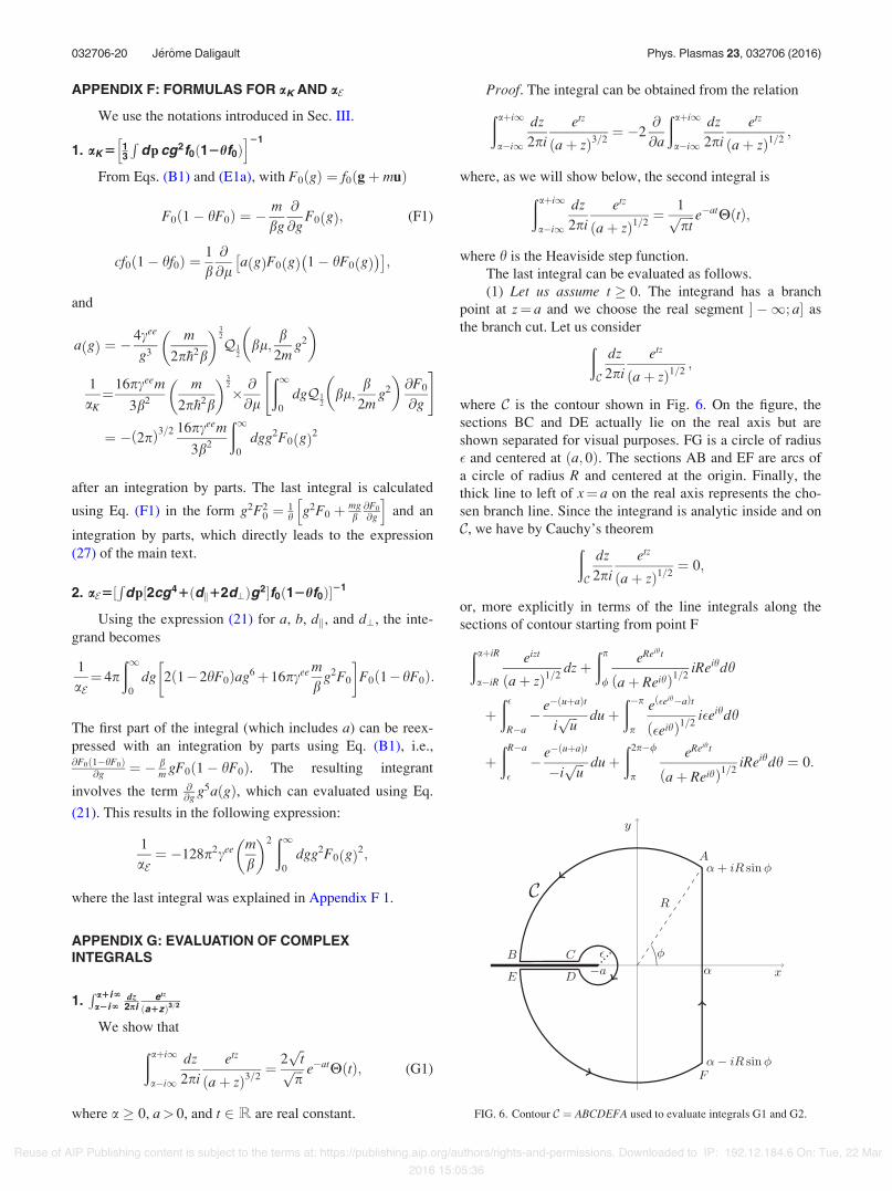
APPENDIX F: FORMULAS FOR aK AND aE

We use the notations introduced in Sec. III.

1. aK 5 13

Rdp cg2f0"12hf0#

h i21

From Eqs. (B1) and (E1a), with F0"g# ! f0"g$ mu#

F0 1) hF0" # ! ) m

bg

@

@gF0 g" #; (F1)

cf0 1) hf0" # ! 1

b@

@la g" #F0 g" # 1) hF0 g" #

* +# $;

and

a g" # ! )4cee

g3

m

2p"h2b

- .32

Q12

bl;b

2mg2

- .

1

aK!16pceem

3b2

m

2p"h2b

- .32

( @

@l

"1

0

dgQ12

bl;b

2mg2

- .@F0

@g

" #

! ) 2p" #3=2 16pceem

3b2

"1

0

dgg2F0 g" #2

after an integration by parts. The last integral is calculated

using Eq. (F1) in the form g2F20 ! 1

h g2F0 $ mgb@F0

@g

h iand an

integration by parts, which directly leads to the expression(27) of the main text.

2. aE5&R

dp&2cg41"dk12d?#g2'f0"12hf0#'21

Using the expression (21) for a, b, dk, and d?, the inte-grand becomes

1

aE! 4p

"1

0

dg 2 1)2hF0" #ag6$16pcee m

bg2F0

% &F0 1)hF0" #:

The first part of the integral (which includes a) can be reex-pressed with an integration by parts using Eq. (B1), i.e.,@F0"1)hF0#

@g ! ) bm gF0"1) hF0#. The resulting integrant

involves the term @@g g5a"g#, which can evaluated using Eq.

(21). This results in the following expression:

1

aE! )128p2cee m

b

- .2 "1

0

dgg2F0 g" #2;

where the last integral was explained in Appendix F 1.

APPENDIX G: EVALUATION OF COMPLEXINTEGRALS

1.R a1i‘a2i‘

dz2pi

etz

"a1z#3=2

We show that

"a$i1

a)i1

dz

2pi

etz

a$ z" #3=2! 2

,,tp,,,pp e)atH t" #; (G1)

where a + 0, a> 0, and t 2 R are real constant.

Proof. The integral can be obtained from the relation

"a$i1

a)i1

dz

2pi

etz

a$ z" #3=2! )2

@

@a

"a$i1

a)i1

dz

2pi

etz

a$ z" #1=2;

where, as we will show below, the second integral is"a$i1

a)i1

dz

2pi

etz

a$ z" #1=2! 1,,,,,

ptp e)atH t" #;

where h is the Heaviside step function.The last integral can be evaluated as follows.(1) Let us assume t + 0. The integrand has a branch

point at z! a and we choose the real segment ' )1; a' asthe branch cut. Let us consider

"

C

dz

2pi

etz

a$ z" #1=2;

where C is the contour shown in Fig. 6. On the figure, thesections BC and DE actually lie on the real axis but areshown separated for visual purposes. FG is a circle of radius! and centered at "a; 0#. The sections AB and EF are arcs ofa circle of radius R and centered at the origin. Finally, thethick line to left of x! a on the real axis represents the cho-sen branch line. Since the integrand is analytic inside and onC, we have by Cauchy’s theorem

"

C

dz

2pi

etz

a$ z" #1=2! 0;

or, more explicitly in terms of the line integrals along thesections of contour starting from point F

"a$iR

a)iR

eizt

a$ z" #1=2dz$

"p

/

eReiht

a$ Reih" #1=2iReihdh

$"!

R)a) e) u$a" #t

i,,,up du$

")p

p

e !eih)a" #t

!eih" #1=2i!eihdh

$"R)a

!) e) u$a" #t

)i,,,up du$

"2p)/

p

eReiht

a$ Reih" #1=2iReihdh ! 0:

FIG. 6. Contour C ! ABCDEFA used to evaluate integrals G1 and G2.



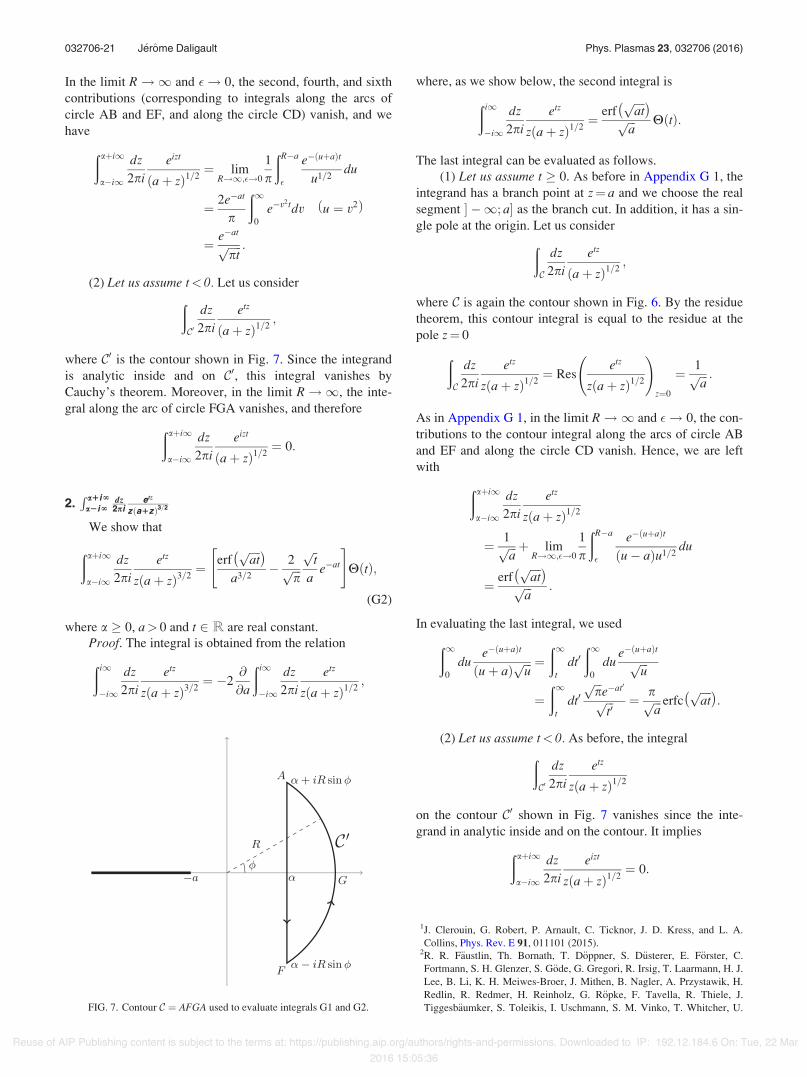
In the limit R!1 and !! 0, the second, fourth, and sixthcontributions (corresponding to integrals along the arcs ofcircle AB and EF, and along the circle CD) vanish, and wehave

"a$i1

a)i1

dz

2pi

eizt

a$ z" #1=2! lim

R!1;!!0

1

p

"R)a

!

e) u$a" #t

u1=2du

! 2e)at

p

"1

0

e)v2tdv u ! v2" #

! e)at

,,,,,ptp :

(2) Let us assume t< 0. Let us consider

"

C0

dz

2pi

etz

a$ z" #1=2;

where C0 is the contour shown in Fig. 7. Since the integrandis analytic inside and on C0, this integral vanishes byCauchy’s theorem. Moreover, in the limit R!1, the inte-gral along the arc of circle FGA vanishes, and therefore

"a$i1

a)i1

dz

2pi

eizt

a$ z" #1=2! 0:

2.R a1i‘a2i‘

dz2pi

etz

z"a1z#3=2

We show that

"a$i1

a)i1

dz

2pi

etz

z a$ z" #3=2! erf

,,,,atp* +

a3=2) 2,,,

pp

,,tp

ae)at

" #

H t" #;

(G2)

where a + 0, a> 0 and t 2 R are real constant.Proof. The integral is obtained from the relation

"i1

)i1

dz

2pi

etz

z a$ z" #3=2! )2

@

@a

"i1

)i1

dz

2pi

etz

z a$ z" #1=2;

where, as we show below, the second integral is

"i1

)i1

dz

2pi

etz

z a$ z" #1=2! erf

,,,,atp* +,,,ap H t" #:

The last integral can be evaluated as follows.(1) Let us assume t + 0. As before in Appendix G 1, the

integrand has a branch point at z! a and we choose the realsegment ' )1; a' as the branch cut. In addition, it has a sin-gle pole at the origin. Let us consider

"

C

dz

2pi

etz

a$ z" #1=2;

where C is again the contour shown in Fig. 6. By the residuetheorem, this contour integral is equal to the residue at thepole z! 0

"

C

dz

2pi

etz

z a$ z" #1=2! Res

etz

z a$ z" #1=2

!

z!0

! 1,,,ap :

As in Appendix G 1, in the limit R!1 and !! 0, the con-tributions to the contour integral along the arcs of circle ABand EF and along the circle CD vanish. Hence, we are leftwith

"a$i1

a)i1

dz

2pi

etz

z a$ z" #1=2

! 1,,,ap $ lim

R!1;!!0

1

p

"R)a

!

e) u$a" #t

u) a" #u1=2du

! erf,,,,atp* +,,,ap :

In evaluating the last integral, we used

"1

0

due) u$a" #t

u$ a" #,,,up !

"1

tdt0"1

0

due) u$a" #t

,,,up

!"1

tdt0

,,,pp

e)at0

,,,t0p ! p,,,

ap erfc

,,,,atp* +

:

(2) Let us assume t< 0. As before, the integral

"

C0

dz

2pi

etz

z a$ z" #1=2

on the contour C0 shown in Fig. 7 vanishes since the inte-grand in analytic inside and on the contour. It implies

"a$i1

a)i1

dz

2pi

eizt

z a$ z" #1=2! 0:

1J. Clerouin, G. Robert, P. Arnault, C. Ticknor, J. D. Kress, and L. A.Collins, Phys. Rev. E 91, 011101 (2015).

2R. R. F#austlin, Th. Bornath, T. D#oppner, S. D#usterer, E. F#orster, C.Fortmann, S. H. Glenzer, S. G#ode, G. Gregori, R. Irsig, T. Laarmann, H. J.Lee, B. Li, K. H. Meiwes-Broer, J. Mithen, B. Nagler, A. Przystawik, H.Redlin, R. Redmer, H. Reinholz, G. R#opke, F. Tavella, R. Thiele, J.Tiggesb#aumker, S. Toleikis, I. Uschmann, S. M. Vinko, T. Whitcher, U.FIG. 7. Contour C ! AFGA used to evaluate integrals G1 and G2.



http://dx.doi.org/10.1103/PhysRevE.91.011101

Zastrau, B. Ziaja, and Th. Tschentscher, Phys. Rev. Lett. 104, 125002(2010).

3Z. Chen, V. Sametoglu, Y. Y. Tsui, T. Ao, and A. Ng, Phys. Rev. Lett.108, 165001 (2012).

4F. Dorchies, V. Recoules, J. Bouchet, C. Fourment, P. M. Leguay, B. I.Cho, K. Engelhorn, M. Nakatsutsumi, C. Ozkan, T. Tschentscher, M.Harmand, S. Toleikis, M. St#ormer, E. Galtier, H. J. Lee, B. Nagler, P. A.Heimann, and J. Gaudin, Phys. Rev. B 92, 144201 (2015).

5A. C. Hayes, G. Jungman, A. E. Schulz, M. Boswell, M. M. Fowler, G.Grim, A. Klein, R. S. Rundberg, J. B. Wilhelmy, D. Wilson, C. Cerjan, D.Schneider, S. M. Sepke, A. Tonchev, and C. Yeamans, Phys. Plasmas 22,082703 (2015).

6A. B. Zylstra, J. A. Frenje, P. E. Grabowski, C. K. Li, G. W. Collins, P.Fitzsimmons, S. Glenzer, F. Graziani, S. B. Hansen, S. X. Hu, M. GatuJohnson, P. Keiter, H. Reynolds, J. R. Rygg, F. H. Sguin, and R. D.Petrasso, Phys. Rev. Lett. 114, 215002 (2015).

7J. A. Frenje, P. E. Grabowski, C. K. Li, F. H. Sguin, A. B. Zylstra, M.Gatu Johnson, R. D. Petrasso, V. Yu Glebov, and T. C. Sangster, Phys.Rev. Lett. 115, 205001 (2015).

8J. C. Fernndez, J. J. Honrubia, B. J. Albright, K. A. Flippo, D. C. Gautier,B. M. Hegelich, M. J. Schmitt, M. Temporal, and L. Yin, Nucl. Fusion 49,065004 (2009).

9Frontiers and Challenges in Warm Dense Matter, Lecture Notes inComputational Science and Engineering Vol. 96, edited by F. Graziani, M.P. Desjarlais, R. Redmer, and S. B. Trickey (Springer, New York, 2014).

10C. A. Ulrich, Time-Dependent Density-Functional Theory, Concepts andApplications (Oxford Graduate Text, 2012).

11F. R. Graziani, V. S. Batista, L. X. Benedict, J. I. Castor, H. Chen, S. N.Chen, C. A. Fichtl, J. N. Glosli, P. E. Grabowski, A. T. Graf, S. P. Hau-Riege, A. U. Hazi, S. A. Khairalla, L. Krauss, A. B. Langdon, R. A.London, A. Markmann, M. S. Murillo, D. F. Richards, H. A. Scott, R.Shepherd, L. G. Stanton, F. H. Streitz, M. P. Surh, J. C. Weisheit, and H.D. Whitley, High Energy Density Physics 8, 105 (2012), and referencestherein.

12H. D. Whitley, Ch. R. Scullard, L. X. Benedict1, J. I. Castor, A. Randles,J. N. Glosli, D. F. Richards, M. P. Desjarlais, and F. R. Graziani, Contrib.Plasma Phys. 55, 192 (2015).

13M. Bonitz, Quantum Kinetic Theory, 2nd ed. (Springer, 2016).14D. Kremp, M. Schlanges, and W.-D. Kraeft, Quantum Statistics of

Nonideal Plasmas (Springer, Heidelberg, 2005).15M. Lampe, Phys. Rev. 170, 306 (1968).16D. R. Nicholson, Introduction to Plasma Theory (John Wiley & Sons, Inc.,

1983).17F. L. Hinton, “Collisional transport in plasma,” in Handbook of Plasma

Physics, Basic Plasma Physics Vol. 1, edited by A. A. Galeev and R. N.Sudan (North-Holland Publishing Co., Amsterdam, 1983), p. 148.

18M. Lemou, Math. Methods Appl. Sci. 23, 1093 (2000).19J. Hu, S. Jin, and B. Yan, Commun. Comput. Phys. 12, 1541 (2012).20J. H. Ferziger and H. G. Kaper, Mathematical Theory of Transport

Processes in Gases (Elsevier, New York, 1972).21S. Brunner, E. Valeo, and J. A. Krommes, Phys. Plasmas 6, 4504 (1999).22P. Danielewicz, Physica 100A, 167 (1980).23E. A. Uehling and G. E. Uhlenbeck, Phys. Rev. 43, 552 (1933).24S. D. Baalrud and J. Daligault, Phys. Plasmas 21, 055707 (2014).25S. D. Baalrud and J. Daligault, Phys. Rev. E 91, 063107 (2015).26J. Daligault, S. D. Baalrud, C. E. Starrett, D. Saumon, and T. Sjostrom,

Phys. Rev. Lett. 116, 075002 (2016).

27F. R. Graziani, J. D. Bauer, and M. S. Murillo, Phys. Rev. E 90, 033104(2014).

28In a dense plasma near equilibrium, an electron with momentumjp1j * pF, where pF is the Fermi momentum, can collide only with anotherelectron whose momenta before and after collision, p2 and p02, both lie onthe thermally “smeared-out” Fermi surface, i.e., "1)H#pF!jp2j;jp2j

0!"1$H#pF, where H ! kBT=EF is the degeneracy parameter.29H. W. Wyld and D. Pines, Phys. Rev. 127, 1851 (1962).30H. Brysk, P. M. Campbell, and P. Hammerling, Plasma Phys. 17, 473

(1975).31W. B. Hubbard and M. Lampe, Astrophys. J. Suppl. 18, 297 (1969).32A. Decoster, P. A. Markowich, and B. Perthame, Modeling of Collisions

(Elsevier, Paris, 1998).33E. E. Salpeter, Aust. J. Phys. 7, 373 (1954).34This is readily shown performing an integration by parts on the second

term in Eq. (3) and writing the first integral as

"dpb V

$

ab %@fa

@pafb 1$ dbhbfb& ' ! @

@pa%"

dpb V$

abfafb 1$ dbhbfb& '

)"

dpb@

@pa% V$

abfafb 1$ dbhbfb& ':

35M. N. Rosenbluth, W. M. MacDonald, and D. L. Judd, Phys. Rev. 107, 1(1957).

36M. Goano, ACM Trans. Math. Software 21, 221 (1995).37We extend the discussion in Ref. 17 to the quantum case.38S. Ichimaru, Statistical Plasma Physics, Basic Principles Vol. I (Westview

Press, 2004), see Sec. 3–5.39In classical plasma physics textbook,17 the assumption on ui ) ue is gener-

ally expressed in terms of the electronic thermal speed ve !,,,,,,,,,,,,,,2=mibi

p, i.e.,

jui ) uej. ve. In many applications, jui ) uej. vi < ve is also satisfied.In general, as previously seen in Sec. II E, the reference electron velocityis max"ve; vF#, and typically vi < ve . vF when electrons are degenerate.The formulas (14) and (17) are obtained assuming jui ) uej. vi, insteadof jui ) uej. vF, as one could wrongly assume from a direct extension ofusual results.

40L. Spitzer, Physics of Fully Ionized Gases (Interscience, New York, 1956).41J. Daligault and G. Dimonte, Phys. Rev. E 79, 056403 (2009), and referen-

ces therein.42A. M. Dimits and B. I. Cohen, Phys. Rev. E 49, 709 (1994).43Z. Lin, W. M. Tang, and W. W. Lee, Phys. Plasmas 2, 2975 (1995).44P. J. Catto and K. T. Tsang, Phys. Fluids 20, 396 (1977).45X. Q. Xu and M. N. Rosenbluth, Phys. Fluids B 3, 627 (1991); see

Appendix A.46H. Grad, Commun. Pure Appl. Math. 2, 325 (1949).47Additional information on orthogonal polynomials with respect to f0"1)

hf0# and their relation to the usual Hermite tensor polynomials can befound in Ref. 49.

48J. Daligault, “Trivariate orthogonal polynomials for quantum kinetictheory,” J. Stat. Phys. (submitted).

49This property can be readily shows by combining the self-adjointnessproperty (28) and the collisional invariants property (29). Indeed, with a !c0 $ c1 % p$ c2p2 and b ! df=f0"1) hf0#, (29) writes as

!dpaC !

&a; b'~0 ! 0 for all b, which is equivalent to &b; a'~0 !!

dpbf0"1)hf0# ~O&af0"1) hf0#' ! 0 8b, and ~O&af0"1) hf0#' ! 0. Here, &a; b'~0 !&a; b'1 $ &a; b'~2.



Documents

On the quantum Landau collision operator and electron ... · On the quantum Landau collision operator and electron collisions in dense plasmas Jer! ^ome Daligaulta) Theoretical Division,