On the Relationship between Decadal Buoyancy Anomalies and Variabilityof the Atlantic Meridional Overturning Circulation

MARTHA W. BUCKLEY,* DAVID FERREIRA, JEAN-MICHEL CAMPIN, JOHN MARSHALL,AND ROSS TULLOCH

Massachusetts Institute of Technology, Cambridge, Massachusetts

(Manuscript received 8 September 2011, in final form 29 February 2012)

ABSTRACT

Owing to the role of the Atlantic meridional overturning circulation (AMOC) in ocean heat transport, AMOC

variability is thought to play a role in climate variability on a wide range of time scales. This paper focuses on the

potential role of the AMOC in climate variability on decadal time scales. Coupled and ocean-only general

circulation models run in idealized geometries are utilized to study the relationships between decadal AMOC

and buoyancy variability and determine whether the AMOC plays an active role in setting sea surface tem-

perature on decadal time scales. Decadal AMOC variability is related to changes in the buoyancy field along the

western boundary according to the thermal wind relation. Buoyancy anomalies originate in the upper ocean of

the subpolar gyre and travel westward as baroclinic Rossby waves. When the buoyancy anomalies strike the

western boundary, they are advected southward by the deep western boundary current, leading to latitudinally

coherent AMOC variability. The AMOC is observed to respond passively to decadal buoyancy anomalies:

although variability of the AMOC leads to meridional ocean heat transport anomalies, these transports are not

responsible for creating the buoyancy anomalies in the subpolar gyre that drive AMOC variability.

1. Introduction

In a recent review paper, Lozier (2010) concluded that

the most significant question concerning variability of the

Atlantic meridional overturning circulation (AMOC) is

the role of the AMOC in creating decadal SST anomalies.

Furthermore, she noted that no observational study to date

has successfully linked SST changes to AMOC variability.

The hypothesis that the AMOC plays an active role in

decadal climate variability is rooted in the role of the

AMOC in the mean meridional ocean heat transport

(OHT). Due to the deep, interhemispheric overturning

circulation in the Atlantic, commonly referred to as the

AMOC, the Atlantic Ocean transports heat northward

in both hemispheres. The Atlantic OHT peaks at a value

of about 1 PW at 208N (Trenberth and Caron 2001;

Ganachaud and Wunsch 2003), and observational (Talley

2003) and modeling (Boccaletti et al. 2005; Ferrari and

Ferreira 2011) studies suggest about 60% of the peak

OHT can be attributed to the AMOC. Thus, the AMOC

plays a role in maintaining the current mean climate, and

it has been suggested that its variability may play a role in

climate variability on a wide range of time scales.

Observations of decadal SST variability from the in-

strumental record (Bjerknes 1964; Kushnir 1994; Knight

et al. 2005; Ting et al. 2009) and climate proxy data (Mann

et al. 1995, 1998) are a second piece of evidence that the

ocean may play an active role in decadal climate vari-

ability. The basin-scale nature of observed decadal SST

anomalies led Bjerknes (1964) and Kushnir (1994) to

hypothesize that these anomalies are due to changes in

meridional OHT. A number of studies have attempted

to test this hypothesis by analyzing the relationships be-

tween decadal SST anomalies and the state of the over-

lying atmosphere. While it is well established that on

interannual time scales SST variability is primarily forced

by local atmospheric variability (Hasselman 1976; Cayan

1992a,b), the relative roles of atmospheric forcing and

ocean dynamics in setting SST on decadal time scales are

not known. Deser and Blackmon (1993) and Seager et al.

(2000) argue that the majority of wintertime SST vari-

ability observed during the last four decades can be ex-

plained as a local passive response to atmospheric forcing.

* Current affiliation: Atmospheric and Environmental Research,

Lexington, Massachusetts.

Corresponding author address: Martha Buckley, 131 Hartwell

Avenue #4, Lexington, MA 02421.

E-mail: marthab@alum.mit.edu

VOLUME 25 J O U R N A L O F C L I M A T E 1 DECEMBER 2012

DOI: 10.1175/JCLI-D-11-00505.1

� 2012 American Meteorological Society 8009

On the other hand, Bjerknes (1964) and Kushnir (1994)

conclude that decadal SST anomalies are not forced by

local atmospheric forcing, and thus the ocean must play

an active role in setting SST on decadal time scales.

Kushnir (1994) suggests that variability of the AMOC is

a likely mechanism for creating the observed decadal

SST anomalies.

The hypothesis that the AMOC may play a role in

climate variability has prompted observational cam-

paigns to monitor the AMOC and meridional OHT

in the Atlantic. Data from the Rapid Climate Change

(RAPID) and Meridional Overturning and Heatflux

Array (MOCHA) observing systems, combined with

wind stress estimates from satellites, has enabled the es-

timation of the AMOC and meridional OHT at 26.58N

since April 2004 (Cunningham et al. 2007; Johns et al.

2010). The success of the RAPID array and studies in-

dicating that the AMOC is not coherent between the

subtropical and subpolar gyres on interannual time scales

(Bingham et al. 2007) have led to proposals for array-

based observing systems at other latitudes, including the

subpolar North Atlantic (OSNAP) and the South Atlantic

at 348S (SAMOC) (Lozier 2010). Additionally, several

arrays in the western basin monitor the deep western

boundary current (DWBC), including Line W off the

coast of New England (Toole et al. 2011) and the Merid-

ional Overturning Experiment (MOVE) array at 168N

(Kanzow et al. 2006). Unfortunately, time series of the

AMOC at 26.58N from the RAPID array are too short to

estimate decadal AMOC variability and observations to

access the meridional coherence of the AMOC are cur-

rently lacking.

The potential role of the AMOC in climate variability

on decadal time scales and the inability of observations

to firmly establish a connection owing to the paucity of

long-term ocean observations have prompted numerous

modeling studies. A plethora of models exhibit AMOC

variability on decadal time scales and find decadal upper-

ocean heat content (UOHC) anomalies associated

with AMOC variability. Many of these studies argue

that the UOHC anomalies are the result of OHT con-

vergence anomalies associated with AMOC variability

(Delworth et al. 1993; Delworth and Mann 2000; Knight

et al. 2005; Zhang et al. 2007; Msadek and Frankignoul

2009). However, correlation does not imply causation, and,

to our knowledge, none of these studies has explicitly

shown that the observed UOHC anomalies are due to

convergence of OHT anomalies resulting from changes

in the AMOC. The observed correlations between

UOHC anomalies and AMOC variability could simply

be due to the thermal wind relation, which relates buoy-

ancy anomalies on the boundaries to AMOC anomalies.

Whether AMOC variability itself plays a role in creating

buoyancy anomalies on the boundaries or these anoma-

lies are the result of other processes is not known.

In this paper we use coupled and ocean-only general

circulation models (GCMs) run in idealized geometries to

study the relationships between decadal AMOC and

buoyancy variability. The models are slight modifications

of the ‘‘Double Drake’’ setup described in Ferreira et al.

(2010, hereafter FMC). As shown in FMC, the mean state

of Double Drake bears an uncanny resemblance to the

current climate, and we will show that the decadal vari-

ability seen in our models has features that resemble more

complex models and the limited observations available.

However, we do not intend to suggest that the models

described here are realistic representations of the real

ocean. Instead, our goal is to carefully examine the rela-

tionships between decadal buoyancy and AMOC vari-

ability, and determine if the AMOC plays an active role in

setting SST on decadal time scales. To our knowledge no

modeling study has unequivocally demonstrated the role of

the AMOC (or the lack thereof) in setting SST on decadal

time scales, despite the obvious importance of this question

and the unique ability of model experiments to answer such

a question. We are, of course, aware that our results may be

model dependent, as is the case with all modeling experi-

ments. As such, we present two different model setups.

We find that despite the different character of MOC and

buoyancy variability in the two models, the relationships

between MOC variability and buoyancy anomalies are

the same, suggesting the robustness of our main results.

In section 2 we describe the models used and their

mean states. In section 3 we explore decadal MOC and

buoyancy variability in our models. Decadal MOC

variability is found to be related to changes in the buoy-

ancy field along the western boundary according to the

thermal wind relation. Buoyancy anomalies originate in

the upper ocean of the subpolar gyre and upon reach-

ing the western boundary, they are advected southward

by the deep western boundary current, leading to latitudi-

nally coherent MOC variability. In section 4, we address

the origin of the decadal buoyancy anomalies, specifically

the role of the MOC, atmospheric forcing, and baroclinic

Rossby waves in creating the buoyancy anomalies. In

section 5 we summarize the results of our modeling

studies and hypothesize how our simple models might be

used as a prism for understanding AMOC variability in

more complex models and in nature.

2. Coupled aquaplanet model

a. Model setup

The model used in this study is the Massachusetts In-

stitute of Technology general circulation model (Marshall

et al. 1997) run in a coupled atmosphere–ocean–sea ice

8010 J O U R N A L O F C L I M A T E VOLUME 25

setup. The model has realistic three-dimensional atmo-

sphere and ocean dynamics, but it is run in idealized ge-

ometry. The planet is covered entirely by water except for

two ridges that extend from the north pole to 348S, di-

viding the ocean into a small basin (almost 908 wide), a

large basin (almost 2708 wide), and a zonally unblocked

southern ocean. As described in FMC, this idealized

Double Drake setup captures the gross features of the

present-day ocean: a meridional asymmetry (circum-

polar flow in the Southern Hemisphere and blocked flow

in the Northern Hemisphere) and a zonal asymmetry (a

small basin and a large basin).

The model setup is the same as is described in FMC.

The atmosphere and ocean are integrated forward on

the same cubed-sphere horizontal grid (Adcroft et al.

2004) at C24 (each face of the cube has 24 3 24 grid

points), yielding a resolution of 3.78 at the equator. The

model uses the following (isomorphic) vertical co-

ordinates: the rescaled pressure coordinate p* for the

atmosphere and the rescaled height coordinate z* for

the Boussinesq ocean (Adcroft and Campin 2004). The

atmosphere is of ‘‘intermediate’’ complexity, employing

the Simplified Parameterization, Primitive Equation

Dynamics (SPEEDY) physics package described in

Molteni (2003). The atmospheric model includes a four-

band radiation scheme, a parameterization of moist

convection, diagnostic clouds, and a boundary layer

scheme. The atmospheric model has low vertical reso-

lution and is composed of five vertical levels.

The ocean has a maximum depth of 3 km and has 15

vertical levels, increasing from a thickness of 30 m at the

surface to 400 m at depth. As eddies are not resolved by

the low-resolution model, the effects of mesoscale

eddies are parameterized as an advective process (Gent

and McWilliams 1990) and an isopynal diffusion (Redi

1982) with a transfer coefficient of 1200 m2 s21 for both

processes. Convective adjustment, implemented as an

enhanced vertical mixing of temperature and salinity, is

used to represent ocean convection (Klinger et al. 1996).

The background vertical diffusivity is uniform and set to

3 3 1025 m2 s21.

Orbital forcing and CO2 levels are prescribed at

present day values. The seasonal cycle is represented,

but there is no diurnal cycle. Fluxes of momentum, heat,

and freshwater are exchanged every hour (the ocean

model time step). The model achieves perfect (machine

accuracy) conservation of freshwater, heat, and salt

during extended integrations, as discussed in Campin

et al. (2008).

Motivated by the work of Winton (1997), who found

that the presence of bottom topography substantially

alters decadal variability in idealized, buoyancy-forced

ocean-only models, we consider two types of bathyme-

try. In one setup, identical to the Double Drake model

analyzed in FMC, the ocean has a uniform depth of 3 km

(henceforth Flat). In the second setup bowl bathymetry

is added to the small basin (henceforth Bowl) so that the

ocean depth varies from 3 km at the center of the basin

to 2.5 km next to the meridional boundaries (see Fig. 1).

Each setup is initialized from rest with temperature and

salinity from a January climatology of the equilibrium

state discussed in FMC and run for 1000 years. To avoid

the (short) adjustment period to the addition of ba-

thymetry, only the last 800 years of these 1000-yr runs

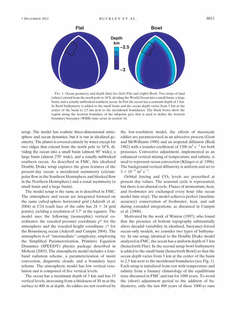
FIG. 1. Ocean geometry and depth (km) for (left) Flat and (right) Bowl. Two strips of land

(white) extend from the north pole to 348S, dividing the World Ocean into a small basin, a large

basin, and a zonally unblocked southern ocean. In Flat the ocean has a constant depth of 3 km.

In Bowl bathymetry is added to the small basin and the ocean depth varies from 3 km at the

center of the basin to 2.5 km next to the meridional boundaries. The black boxes show the

region along the western boundary of the subpolar gyre that is used to define the western

boundary buoyancy (WBB) time series in section 3d.

1 DECEMBER 2012 B U C K L E Y E T A L . 8011

are analyzed. Since our interest is decadal variability,

annual average outputs are analyzed.

b. Mean state

Here we briefly describe the very similar mean states of

Flat and Bowl (see FMC for a detailed analysis of Flat,

i.e., Double Drake). As discussed in FMC, the small basin

is saltier than the large basin, similar to the higher salinity

of the Atlantic relative to the Pacific. Although the higher

sea surface salinity (SSS) in the small basin is partially

compensated by warmer SST, the surface density is

higher in the small basin than in the large basin. As a re-

sult, deep convection is restricted to the small basin (see

Fig. 10 in FMC).

The zonal-mean zonal surface wind stress, shown in the

left panels of Fig. 2, is easterly in the tropics, westerly in

midlatitudes, and easterly near the poles. This large-scale

pattern of wind stress forces the ocean’s gyre circulations

and subtropical overturning cells. In steady state, neglect-

ing friction, the vertically integrated vorticity equation is

bV 51

ro

curlzt 11

ro

curlz( pb$h), (1)

where h(x, y) is the depth of the ocean, pb is the bottom

pressure, and b is the meridional gradient of the Cori-

olis parameter. The vertically integrated meridional

velocity V is determined by two terms: the vertical com-

ponent of the wind stress curl (first term on the right) and

the bottom pressure torque (second term on the right).

The colored contours in Fig. 2 show the windstress curl

(middle panels) and bottom pressure torque (bottom-

right panel) in the small basin. In Flat V is determined

solely by the wind stress curl, leading to a barotropic

streamfunction that is cyclonic in the subpolar gyre and

anticyclonic in the subtropical gyres and ‘‘polar’’ gyre, the

FIG. 2. (left) Average zonal-mean zonal wind stress in (top) Flat and (bottom) Bowl. (middle) Mean wind stress

curl (colors) and horizontal currents at the surface (vectors) in the small basin for (top) Flat and (bottom) Bowl.

(right) Mean bottom pressure torque (colors) and horizontal currents at a depth of 1735 m (vectors) for (top) Flat and

(bottom) Bowl.

8012 J O U R N A L O F C L I M A T E VOLUME 25

region of negative wind stress curl north of 648N. In Bowl

the bottom pressure torque term is significant on the

western boundary of the subpolar gyre and in the polar

gyre. In the polar gyre the positive bottom pressure

torque term is larger than the negative windstress curl,

leading to a cyclonic barotropic streamfuction.

The vectors in Fig. 2 show the mean currents in the

small basin at the surface (middle panels) and at a depth of

1735 m (right panels). The surface circulation is anticy-

clonic in the subtropical gyres and cyclonic in the subpolar

gyre. At the surface the cyclonic subpolar gyre extends

to the north pole in both Flat and Bowl. The strongest

surface currents are found along the western boundary,

except in the subpolar gyre where the strongest currents

are along the eastern boundary. Deep-water formation in

the small basin feeds a DWBC, which flows southward

from 648N to the exit of the small basin.

As a result of deep-water formation, a deep meridional

overturning circulation develops in the small basin, similar

to the overturning circulation in the present-day Atlantic

Ocean. The residual-mean overturning streamfunction

(the sum of the Eulerian and parameterized eddy-induced

streamfunctions) in the small basin (henceforth called

the MOC) in Flat and Bowl are plotted in the left panels

of Fig. 3.1 The majority of the water that sinks in the

small basin is still at depth when it exits the small basin,

indicating that deep water upwells primarily in the

southern ocean (and to a lesser extent in the large basin).

In contrast, the MOC in the large basin (see Fig. 6 in

FMC) is dominated by shallow wind-driven cells.

The meridional OHTs in the small and large basins of

the model bear a striking similarity to those observed in

the Atlantic and Indo-Pacific basins of the modern cli-

mate (see Fig. 2 in FMC). Like in the Indo-Pacific basin,

the OHT in the large basin is due to the gyre circulations

and Ekman transports and is poleward in both hemi-

spheres. Similar to the Atlantic, the OHT transport in the

small basin is northward in both hemispheres (see Fig. 4)

because of the presence of a deep overturning cell.

In summary, the mean states of Flat and Bowl have

many similarities to the present climate. Specifically, the

small basin is saltier than the large basin and a deep,

FIG. 3. (left) The residual mean MOC in the small basin (colors) and the MOC diagnosed from Eq. (5) (black/white contours) for (top)

Flat and (bottom) Bowl. White (black) contours correspond to a positive (negative) MOC and the contour interval for both colors and

black/white contours is 4 Sv. The black box shows the latitude and depth range (88–608N, 460–1890-m depth) used to define the MOC time

series. (middle) A 100-yr segment of anomalies of the yearly MOC time series (black) and reconstructed MOC time series [diagnosed from

Eq. (5), blue] for (top) Flat and (bottom) Bowl. (right) The spatial patterns of MOC variability obtained by projecting MOC anomalies

onto the MOC index (colors) and projecting MOC anomalies diagnosed from Eq. (5) onto the reconstructed MOC index (black/white

contours) for (top) Flat and (bottom) Bowl. White (black) contours correspond to positive (negative) MOC anomalies and the contour

interval for both the colors and black/white contours is 0.1 Sv.

1 In Bowl bottom pressure torques potentially play a role in

setting the pathways of the mean MOC, as discussed in a recent

paper by Spence et al. (2012), although they found the effects to be

largest in high-resolution models.

1 DECEMBER 2012 B U C K L E Y E T A L . 8013

interhemispheric MOC develops in the small basin. Our

focus is on the small basin, which can be thought of as an

idealized Atlantic Ocean.

3. Decadal MOC and buoyancy variability

a. Decadal MOC variability

The MOC in the box from 88 to 608N, 460 to 1890-m

depth (box shown in black in left panels of Fig. 3) is used

as a measure of the large-scale MOC variability. At each

latitude, a yearly time series of the MOC is computed by

taking the value of the MOC at the depth of the maxi-

mum of the mean MOC within the box. These time se-

ries are then averaged over all the latitudes in the box to

create a MOC time series. The middle panels of Fig. 3

show 100-yr segments of yearly anomalies of the MOC

time series for Flat (top) and the Bowl (bottom).

This definition of the MOC time series is chosen to

focus our attention on large-scale (latitudinally coherent)

MOC variability, and the analysis presented here is not

sensitive to the box chosen. If instead a subtropical box

spanning the equator (88S–408N) is chosen, variability of

the resulting MOC time series (henceforth the subtropical

MOC time series) is almost identical (correlation at

lag 0 is 0.94 for Flat and 0.90 for Bowl). Thus, the low-

frequency MOC variability seen in our model is coherent

between the subtropical and subpolar gyres and across the

equator. On shorter (intraannual) time scales the MOC

variability in the model does not exhibit such strong lat-

itudinal coherence, as was noted by Bingham et al. (2007).

The right panels of Fig. 3 show the spatial patterns of

MOC variability obtained by projecting MOC anoma-

lies onto the normalized MOC time series (henceforth

called the MOC index).2,3 Each spatial pattern is in-

terhemispheric and strongly resembles the first empiri-

cal orthogonal function (EOF) of the MOC (calculated

over the latitude range 208S to 608N, not shown), which

explains 54% of the variance for Flat and 40% of the

variance for Bowl. The MOC time series is highly cor-

related with the first principle component (PC) time

series of the MOC (correlation is 0.96 for Flat and 0.85

for Bowl), further confirming that the MOC time series

captures the large-scale MOC variability.

The power spectrum of the MOC index in Flat (top-

left panel of Fig. 5) is red at high frequencies, has a large

peak at a period of about 34 yr, and flattens out at low

frequencies. The power spectrum of the MOC index in

Bowl (bottom-left panel of Fig. 5) is red at high fre-

quencies and flattens out at low frequencies. The tran-

sition from a red spectrum to a flat spectrum occurs at

a time scale of approximately 24 yr.

To examine the spatial and temporal variability of the

MOC anomalies, the MOC index is projected onto MOC

anomalies at various lags (see right panels of Figs. 6 and 7).

Figure 8 (colors) shows MOC anomalies at the depth of

the maximum of the mean MOC as a function of latitude

and lag. In both Flat and Bowl, MOC anomalies originate

in the subpolar gyre and travel southward with time.

Figure 4 shows the OHT anomalies that are associated

with a positive MOC anomaly. OHT anomalies of 0.04

PW are associated with MOC anomalies with a standard

deviation of 1 Sv (Sv [ 106 m3 s21). These OHT anom-

alies are in accord with decadal OHT anomalies observed

in more realistic climate models. In the Hadley Centre

Coupled Model, version 3 (HadCM3) decadal OHT

anomalies of 0.04 PW are associated with MOC anomalies

O(1 Sv) (Dong and Sutton 2001, 2003; Shaffrey and Sut-

ton 2006). In the National Center for Atmospheric Re-

search Community Climate System Model, version 3

(CCSM3) decadal OHT anomalies (amplitude of 0.12

PW) are associated with MOC anomalies with an ampli-

tude of 4.5 Sv (Danabasoglu 2008).

FIG. 4. Mean meridional ocean heat transport (OHT, black lines,

left ordinate) and OHT anomalies associated with a positive MOC

anomaly (gray lines, right ordinate) for (top) Flat and (bottom) Bowl.

OHT anomalies associated with decadal MOC variability are com-

puted by projecting OHT anomalies onto the MOC index at lag 0.

2 Projecting a data field onto a time series is equivalent to

computing the covariance between the time series and the data

field at each spatial location.3 A normalized time series has a mean of zero and standard

deviation of one.

8014 J O U R N A L O F C L I M A T E VOLUME 25

b. Diagnosis of MOC variability from thermal windrelation and Ekman transports

To examine the origin of the MOC variability observed

in the model, we decompose the meridional velocity y into

geostrophic and Ekman components (Lee and Marotzke

1998; Hirschi and Marotzke 2007): y 5 yg 1 yEk. The

geostrophic velocity yg is calculated from the buoyancy

field b using the vertically integrated thermal wind relation:

yg(z) 51

f

ðz

2h

›b

›xdz 1 yb, (2)

in which f is the Coriolis parameter, h(x, y) is the

ocean depth, and yb is the unknown meridional bottom

velocity. The Ekman velocity yEk is related to the zonal

surface windstress tx as

yEk 5 2tx

ro f dz(3)

in which ro is a reference density and dz is the thickness

of the Ekman layer (or top model layer). The mass

conservation constraint can be used to solve for the

zonal-average bottom velocity yb. We find

yb 5 21

A

ðxe

xw

dx

ð0

2h

1

f

ðz

2h

›b

›xdz 1 yEk

� �dz, (4)

FIG. 5. (left) Power spectra P( f ) of the MOC index (gray) and the WBB index (black) for (top) Flat and (bottom)

Bowl. Dashed vertical lines indicate the time scale of the peak in Flat and the time scale at which the transition from

a red spectrum to a flat spectrum occurs in Bowl. Dashed diagonal lines show a fit to the red portion (1/f , 24 yr) of

the spectrum of the WBB index: P( f ) 5 Cf 2a. We find a 5 2.21 for Flat and a 5 2.24 for Bowl. (right) Lagged

correlation between MOC index and WBB index for (top) Flat and (bottom) Bowl. Lag 5 0 corresponds to the

maximum MOC index. Open circles indicate the lags for which spatial fields are plotted in Figs. 6 and 7.

1 DECEMBER 2012 B U C K L E Y E T A L . 8015

where A is the area of the longitude–depth section. A

streamfunction can then be computed by integrating y

zonally and vertically:

~C(z) 5

ðxe

xw

dx

ðz

2hy dz. (5)

The left panels of Fig. 3 (contours) show the mean

MOC diagnosed according to Eq. (5). The spatial cor-

relation between the mean Eulerian4 MOC and the

MOC estimate is 0.81 for Flat and 0.82 for Bowl. Errors

are largely due to errors in determining the barotropic

flow, but the neglect of friction and nonlinearity also

play a role.5 The center panels of Fig. 3 compare the

variability of the actual MOC time series (MOC in the box

from 88 to 608N, 460 to 1890-m depth) to the variability of

the reconstructed MOC time series [MOC in same box,

but when the MOC is calculated from Eq. (5)]. Despite

the errors in diagnosing the mean MOC, MOC vari-

ability in the reconstruction matches the actual MOC

variability almost exactly (correlation is 0.95 for Flat

and 0.90 for Bowl).

The right panels of Fig. 3 (contours) show the spatial

patterns of MOC variability obtained by projecting the

reconstructed MOC anomalies onto the normalized

FIG. 6. Flat: (left) east–west sections of buoyancy and air–sea buoyancy flux anomalies at 608N, (middle) buoyancy anomalies along the

western and eastern boundaries of the small basin, and (right) MOC anomalies projected onto the MOC index at at various lags. Buoyancy and

MOC anomalies are shown for (top) lag 5 28 yr, (middle) lag 5 24 yr, and (bottom) lag 5 0 yr. Air–sea buoyancy flux anomalies are shown

one year earlier to demonstrate that air–sea buoyancy fluxes damp the decadal buoyancy anomalies. Only covariances significant at the 95%

confidence level are plotted. The thin black lines in the middle panels show the mean isopynals along the western and eastern boundaries.

4 When computing spatial correlations, we compare the re-

constructed MOC to the Eulerian MOC rather than the residual

MOC since the bolus part cannot be estimated from the thermal

wind relation. However, in the small basin, the mean Eulerian and

residual MOC are very similar (spatial correlation is 0.98 for Flat

and 0.97 for Bowl).

5 If we instead diagnose the MOC from the pressure field, which

does not require us to estimate the barotropic flow from mass

conservation, the MOC estimate improves markedly. The spatial

correlation between the mean MOC and the MOC estimate im-

proves to 0.96 for both Flat and Bowl. Additionally, the vertical

structure of the MOC, including the subtropical cells, is properly

represented.

8016 J O U R N A L O F C L I M A T E VOLUME 25

reconstructed MOC time series (henceforth called the

reconstructed MOC index). The spatial correlation be-

tween the reconstructed MOC variability and the actual

MOC variability is 0.97 for Flat and 0.92 for Bowl. The

spatial and temporal variability of the MOC and the

reconstructed MOC are compared in Fig. 8, which shows

MOC anomalies at the depth of the maximum of the

mean MOC as a function of latitude and lag. The re-

constructed MOC variability (contours) matches the ac-

tual decadal MOC anomalies (colors) almost exactly

except in the high northern latitudes. The calculation is

less accurate in the high northern latitudes owing to the

small number of grid points in the northern apex of the

small basin. Additionally, the flow may not be geostrophic

near the boundaries due to the friction and inertial effects.

In summary, while there are substantial errors in esti-

mating the mean MOC from Eq. (5), it is an extremely

accurate method for diagnosing MOC variability, a fact

which has been noted by other studies (Hirschi and

Marotzke 2007). The primary reason for the errors in

the mean MOC is that the barotropic flow is difficult to

estimate in regions where bottom velocities are not small

(Baehr et al. 2004). However, although bottom velocities

are often not small, their variability on decadal time scales

tends to be quite small, so errors in estimating the baro-

tropic flow do not affect our estimates of MOC variability.

1) ROLE OF GEOSTROPHIC AND EKMAN

TRANSPORTS

To examine the relative contributions of geostrophic

and ageostrophic (Ekman) velocities to decadal MOC

variability, we calculate C9tw

, the decadal MOC anomalies

expected from the thermal wind contribution alone (set-

ting y9Ek 5 0). The streamfunction C9tw

is indistinguishable

from ~C9 (not shown), demonstrating that decadal MOC

anomalies are related to buoyancy anomalies on the

boundaries according to the thermal wind relation, and

ageostrophic MOC anomalies due to Ekman transport

variability are negligible on decadal time scales. Our

results are in accord with previous modeling studies (Sime

et al. 2006; Hirschi and Marotzke 2007; Hirschi et al. 2007)

and analyses of ocean state estimates (Cabanes et al.

2008), which found that Ekman transport variability

plays a role in AMOC variability on short time scales,

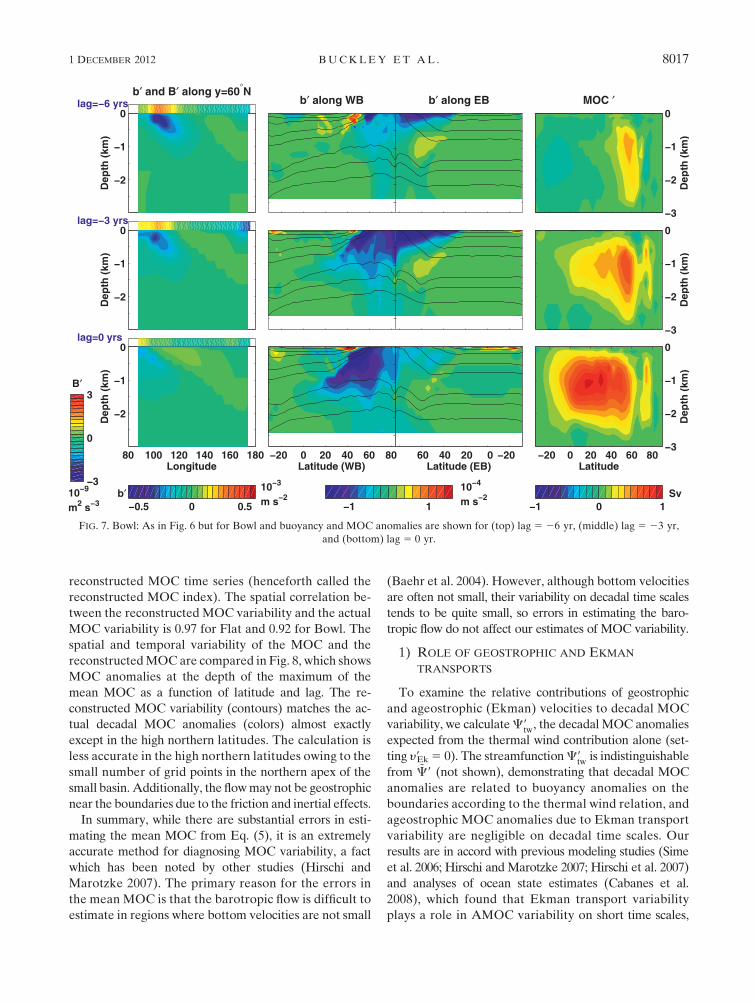
FIG. 7. Bowl: As in Fig. 6 but for Bowl and buoyancy and MOC anomalies are shown for (top) lag 5 26 yr, (middle) lag 5 23 yr,

and (bottom) lag 5 0 yr.

1 DECEMBER 2012 B U C K L E Y E T A L . 8017

while AMOC variability on longer (interannual to

decadal) time scales is primarily related to changes in

the density field.

2) ROLE OF WESTERN AND EASTERN

BOUNDARIES

To examine the relative roles of buoyancy anomalies

at the western and eastern boundaries in contributing to

MOC variability, we project buoyancy anomalies on the

western and eastern boundaries onto the MOC index at

various lags (see middle panels of Figs. 6 and 7). In the

subpolar gyre both the eastern and western boundaries

play a role in MOC variability in Flat, whereas only the

contribution of the western boundary is important in

Bowl. Outside the subpolar gyre MOC anomalies in

both Flat and Bowl are due to buoyancy anomalies on

the western boundary. Prior to the maximum MOC

anomaly, a negative buoyancy anomaly reaches the

western boundary of the subpolar gyre. The buoyancy

anomaly travels southward following the mean isopynals,

leading to latitudinally coherent MOC variability. Be-

cause of the slow travel of the buoyancy anomalies down

the western boundary (approximately 2 cm s21) and their

path along the mean isopynals, we hypothesize that the

anomalies are advected southward by the DWBC. The

advective nature of the travel of buoyancy anomalies is in

accord with observational results tracking potential vortic-

ity anomalies (Curry et al. 1998; Pena-Molino et al. 2011)

and several modeling studies (Marotzke and Klinger 2000;

Zhang 2010), but in contrast to numerous theoretical

studies that implicate Kelvin waves in the southward com-

munication of AMOC variability (Kawase 1987; Johnson

and Marshall 2002a,b; Deshayes and Frankignoul 2005).

c. Summary

In summary, our model exhibits large-scale, latitudi-

nally coherent MOC variability on decadal time scales.

Decadal MOC anomalies are related to buoyancy

anomalies on the boundaries in accord with the thermal

wind relation. Outside the subpolar gyre anomalies on

the eastern boundary are negligible, and thus MOC

variability is determined solely by buoyancy anomalies

on the western boundary. Western boundary buoyancy

anomalies are first seen in the subpolar gyre and sub-

sequently travel southward along the western boundary,

following the mean isopynals.

d. Decadal buoyancy anomalies

Projecting subsurface buoyancy anomalies onto the

MOC index at various lags demonstrates that upper-

ocean buoyancy anomalies in the subpolar gyre are as-

sociated with decadal MOC variability. The left panels

of Figs. 6 and 7 show buoyancy and air–sea buoyancy

flux anomalies through 608N (the latitude of the maxi-

mum buoyancy anomalies) projected onto the MOC

index at various lags. The buoyancy anomalies, which

are O(1023 m s22) near the surface and decay with depth,

are dominated by temperature anomalies (0.88C in Flat,

0.58C in Bowl) and associated with smaller compensating

salinity anomalies (0.065 psu in Flat, 0.036 psu in Bowl). In

Flat buoyancy anomalies originate along the eastern

boundary and propagate westward. In Bowl buoyancy

anomalies appear to originate in the interior of the

gyre near the western boundary. When these buoyancy

anomalies strike the western boundary, they are ad-

vected southward by the DWBC, resulting in MOC

variability in thermal wind balance with the buoyancy

anomalies on the boundary, as described in section 3b.

The importance of buoyancy anomalies on the west-

ern boundary to MOC variability led us to define a time

series of western boundary buoyancy. Annual-mean

buoyancy anomalies are averaged over a box along the

western boundary between 408 and 658N latitude (box

shown in black in Fig. 1) from 130- to 320-m depth to

compute a western boundary buoyancy (WBB) time

series. One-hundred-year segments of the WBB time

FIG. 8. MOC anomalies at the depth of the maximum of the

mean MOC (below 460 m) as a function of latitude and lag for

(top) Flat and (bottom) Bowl. Colors show the actual MOC

anomalies and contours show MOC anomalies calculated from

buoyancy and windstress fields according to Eq. (5). Black (white)

contours indicate positive (negative) MOC anomalies. The contour

interval is 0.1 Sv for Flat and 0.05 Sv for Bowl for both the colors

and black/white contours.

8018 J O U R N A L O F C L I M A T E VOLUME 25

series are plotted in black in Fig. 9. The power spectra of

the normalized WBB time series (henceforth the WBB

index) are plotted in the left panels Fig. 5. In both Flat

and Bowl, the power spectrum of the WBB index is very

similar to the power spectrum of the MOC index. The

right panels of Fig. 5 show the lagged correlation between

the MOC index and the WBB index. Negative buoyancy

anomalies on the western boundary precede the maxi-

mum MOC anomaly by 4 yr in Flat and 6 yr in Bowl.

4. Origin of buoyancy anomalies

Our analysis thus far has demonstrated that decadal

MOC anomalies are related to buoyancy anomalies that

originate in the subpolar gyre. In this section we explain

the origin of the buoyancy anomalies in the subpolar

gyre.

a. Role of air–sea heat fluxes

The left panels of Figs. 6 and 7 show buoyancy and air–

sea buoyancy flux anomalies through 608N (the latitude

of the maximum buoyancy anomalies) projected onto the

MOC index at various lags. Air–sea buoyancy fluxes

O(4 3 1029 m2 s23) are associated with decadal buoyancy

anomalies O(1023 m s22). The buoyancy fluxes are domi-

nated by heat fluxes, which have a maximum magnitude of

8 W m22 in Flat and 6 W m22 in Bowl. Air–sea buoyancy

fluxes damp the buoyancy anomalies at all stages of the

evolution of the buoyancy anomalies. Previous observa-

tional (Deser and Blackmon 1993; Kushnir 1994; Dong

and Kelly 2004; Dong et al. 2007) and modeling (Dong and

Sutton 2003; Shaffrey and Sutton 2006; Grist et al. 2010)

studies also found that on short time scales upper-ocean

temperature anomalies are forced by air–sea heat fluxes,

while on long time scales the ocean circulation plays a role

in creating temperature anomalies, which are then damped

by air–sea heat fluxes.

b. Role of the MOC in creating decadal buoyancyanomalies

In this section we will address whether the MOC plays

an active role in creating decadal buoyancy anomalies in

FIG. 9. Plot of the WBB time series (black curves) and Hovmoller plot of subsurface (depth 265 m) buoy-

ancy anomalies averaged over the latitude range 558–658N (colors) for (left) Flat and (right) Bowl. Black lines on

Hovmoller plot for Flat show an estimate of the westward phase velocity of the buoyancy anomalies.

1 DECEMBER 2012 B U C K L E Y E T A L . 8019

the subpolar gyre. We conduct an ocean-only experi-

ment in which we suppress variability of the large-scale

MOC and determine if buoyancy anomalies in the sub-

polar gyre are altered. The ocean model is initialized

with a state from the spunup coupled model and forced

with 5-day mean time series of heat, freshwater, and

momentum fluxes from the coupled model as well as

restoring of SST and SSS to that of the coupled run on

time scales of 71 days and 1 year, respectively.6 Along

the western boundary south of 508N temperature and

salinity are restored to climatology throughout the water

column with a restoring time scale of two months. This

restoring at depth suppresses the large-scale MOC var-

iability since the MOC is concentrated on the western

boundary but does not directly alter temperature and

salinity in the subpolar gyre where the buoyancy anom-

alies originate. This experiment will be referred to as

RESTORE-WB.

The top panels of Fig. 10 show the subtropical MOC

time series for the coupled run and the RESTORE-WB

experiment. We chose a box (88S–408N, 460–1890-m

depth) that excludes the subpolar gyre to define our

MOC time series since we are interested in understanding

if MOC anomalies outside the subpolar gyre play a role

in creating the buoyancy anomalies in the subpolar gyre.

Restoring temperature and salinity along the western

boundary greatly reduces the amplitude of subtropical

MOC variability in both Flat and Bowl. The modest

MOC variability observed in the RESTORE-WB

FIG. 10. (top) Yearly subtropical MOC time series in the coupled model (black curve) and ocean-only model

experiment RESTORE-WB (gray curve) and (bottom) WBB time series in the coupled model (black curve) and

RESTORE-WB (gray curve): (left) Flat and (right) Bowl.

6 Restoring of SST and SSS is needed for the ocean-only model

to accurately reproduce the coupled model trajectory since

a number of nonlinear processes, such as convective events, are not

well represented when the ocean model is forced with 5-day av-

eraged forcing. If no restoring is included, the ocean-only model

trajectory slowly diverges from that of the coupled model. These

differences substantially affect the MOC and WBB time series

after approximately 70 years.

8020 J O U R N A L O F C L I M A T E VOLUME 25

experiment is primarily due to variability in Ekman

transport forced by wind variability (not shown). The

bottom panels of Fig. 10 show buoyancy anomalies av-

eraged over a box near the western boundary of the

subpolar gyre.7 Although MOC variability has been

suppressed substantially, the buoyancy anomalies near

the western boundary of the subpolar gyre remain vir-

tually unchanged.

From this experiment we conclude that although

large-scale MOC variability does lead to OHT anoma-

lies (see Fig. 4), these transports are not responsible for

creating the buoyancy anomalies in the subpolar gyre

that drive the MOC variability. In both Flat and Bowl

the large-scale MOC responds passively to buoyancy

anomalies that originate in the subpolar gyre. Of course

variability of the velocity field (and hence the MOC) and

buoyancy field in the subpolar gyre are tightly coupled

according to the thermal wind relation. The point here is

that variability of the large-scale MOC (outside the

subpolar gyre) and the resulting OHT anomalies do not

play a role in creating the buoyancy anomalies seen in

the subpolar gyre. These anomalies are formed by pro-

cesses local to the subpolar gyre. Thus, if we can explain

the origin of these buoyancy anomalies, we will suc-

cessfully explain the mode of MOC variability.

c. Role of atmospheric forcing

To determine if stochastic atmospheric forcing is

needed to excite buoyancy and MOC variability, we

conduct an ocean-only experiment in which the ocean is

forced with climatological forcing. In the experiment,

which we will refer to as CLIM-DAMP, the ocean model

is forced with 5-day climatological (100-yr average from

coupled model) forcing of heat, momentum, and fresh-

water and damping of SST to climatology with the ca-

nonical value of 20 W m22 K21 (Frankignoul et al. 1998).

The MOC time series from CLIM-DAMP is compared

to the MOC time series from the coupled run in Fig. 11.

For Flat CLIM-DAMP reproduces the low-frequency

MOC variability of the coupled model amazingly well.

If realistic damping is not included in the ocean-only

experiment, the decadal MOC variability is much larger

than in the coupled model (not shown). Thus, the decadal

mode of variability observed in Flat is a self-sustained

ocean-only mode damped by air–sea heat fluxes. For

Bowl MOC variability rapidly decays in CLIM-DAMP.

In the presence of realistic damping by air–sea heat

fluxes, decadal MOC and buoyancy variability does not

exist without continuous excitation by stochastic atmo-

spheric forcing.

An additional experiment CLIM-WEAK-DAMP in

which damping of SST anomalies was set to be only

4 W m22 K21 demonstrates that if damping of SST

anomalies is weak enough, MOC variability persists in

Bowl even in the absence of stochastic atmospheric

forcing. Although the MOC variability observed in Bowl

in the CLIM-WEAK-DAMP experiment is quite regular,

like that of the experiment CLIM-DAMP in Flat, the

spatial pattern of the buoyancy variability in CLIM-

WEAK-DAMP is very different to that observed in

Flat. The buoyancy variability in Bowl in both CLIM-

WEAK-DAMP and the coupled model is maximal

near the western boundary of the subpolar gyre. In con-

trast, in Flat buoyancy anomalies originate near the

eastern boundary and propagate westward in both

the CLIM-DAMP experiment and the coupled model.

Thus, adding bathymetry has not merely increased dis-

sipation, leading to damped rather than self-sustained

modes, it has fundamentally altered the character of the

variability.

FIG. 11. Yearly subtropical MOC time series in the coupled

model (solid black curve) and ocean-only model experiment

CLIM-DAMP (dashed black curve) for (top) Flat and (bottom)

Bowl. For Bowl an additional experiment, CLIM-WEAK-DAMP

is shown (gray curve). CLIM-WEAK-DAMP is the same as CLIM-

DAMP, but the damping of SST anomalies is set to be 4 W m22 K21

rather than the canonical value of 20 W m22 K21.

7 The box is the same as shown in Fig. 1 (408N and 658N, 130–320-m

depth), but the points immediately adjacent to the western boundary

have been removed since temperature and salinity are restored to

climatology along the western boundary.

1 DECEMBER 2012 B U C K L E Y E T A L . 8021

Additional ocean-only experiments (not shown) dem-

onstrate that in Bowl both stochastic wind and buoyancy

forcing are capable of exciting the mode of buoyancy and

MOC variability. Thus, we conclude that the decadal

buoyancy and MOC variability in Bowl is due to damped

ocean-only mode(s) excited by stochastic atmospheric

forcing.

d. Creation of buoyancy variance

In this section we will show that decadal buoyancy

anomalies extract energy out of the mean flow, which

allows them to grow. Taking the time mean (denoted by

overbars) of the linearized buoyancy variance equation,

one can show that, in order for a mode to grow against

mixing and damping by air–sea buoyancy fluxes, the

term 2u9b9 � $b must be positive averaged over the

domain (Colin de Verdiere and Huck 1999). Here u

and b are the mean velocity and buoyancy fields and u9

and b9 are the deviations from the time mean fields.8

In Flat 2u9b9 � $b . 0 in a broad region near the

eastern boundary and also along the western bound-

ary of the subpolar gyre (see left panel of Fig. 12). In

Bowl 2u9b9 � $b . 0 only along the western boundary

of the subpolar gyre (see right panel of Fig. 12). In

both models the domain average of 2u9b9 � $b . 0,

indicating that perturbations can grow by extracting

energy from the mean flow. Unfortunately, it is more

difficult to conclude where in the domain the pertur-

bations are actually extracting energy from the mean

flow. Locally, 2u9b9 � $b . 0 can mean either that

perturbations are extracting energy from the mean

flow locally or that waves are transporting variance to

that location.

e. Propagation of buoyancy anomalies

Hovmoller plots of yearly subsurface buoyancy

anomalies averaged over the latitude range 558–658N, the

latitude range of the maximum buoyancy anomalies, are

shown as a function of longitude and time in Fig. 9. In Flat

buoyancy anomalies originate near the eastern boundary

and propagate westward, taking approximately 34 years

to cross the basin (average velocity of 20.47 cm s21).

Buoyancy anomalies move slower c ’ 20.35 cm s21

in the eastern part of the basin and speed up to c ’

20.87 cm s21 as they approach the western boundary.

While there is some evidence of westward propagation

in Bowl, the largest buoyancy anomalies are confined to

the region near the western boundary. The ubiquity of

westward propagation led us to ask if the buoyancy

variability in the model can be explained by a Rossby

wave model. A number of studies have previously shown

that Rossby wave models forced by windstress anomalies

successfully capture much of the observed sea surface

height and thermocline depth variability measured by

tide gauges (Sturges and Hong 1995), hydrographic data

(Sturges et al. 1998; Schneider and Miller 2001), and sat-

ellite altimetry (Fu and Qui 2002; Qiu 2002; Qiu and Chen

2006). Details of the Rossby wave model are described in

the appendix.

The left panels of Fig. 13 show baroclinic pressure

potential anomalies p9bc (pressure potential anomalies

FIG. 12. The production of buoyancy variance 2u9b9 � $b in (left) Flat and (right) Bowl.

Thick black line is at the equator and thin black lines show the lines of zero windstress curl in

the Northern Hemisphere (208, 408, and 648N).

8 We avoid the terminology ‘‘eddy’’ creation of buoyancy vari-

ance, used by Colin de Verdiere and Huck (1999), since in our

coarse resolution model eddies are not resolved. In parameterizing

the eddies it is assumed that the eddy buoyancy flux (u*b*) is down

the mean buoyancy gradient: 2u*b* 5 2Ke$b, where Ke is the

eddy diffusivity. Therefore, the effect of the parameterized eddies

(which was not included in our calculation) 2u*b* � $b . 0 ev-

erywhere.

8022 J O U R N A L O F C L I M A T E VOLUME 25

projected onto the first baroclinic mode) in the model

averaged over the latitude range 558–658N as a function

of longitude and time. Note the similarity between the

p9bc

and the buoyancy anomalies at a depth of 265 m

(see Fig. 9). Positive (negative) buoyancy anomalies are

associated with a thicker (thinner) thermocline and high

(low) sea surface heights, and thus a positive (negative)

value of p9bc. The right panels of Fig. 13 show p9r, the

baroclinic pressure potential anomalies calculated from

the Rossby wave model. The Rossby wave model suc-

cessfully captures the basic character of p9bc

in both Flat

and Bowl. In Flat westward-propagating pressure (and

buoyancy) anomalies are found over the entire width

of the basin. In Bowl the largest baroclinic pressure

anomalies are restricted to the western part of the basin.

Furthermore, the Rossby wave model can be used to

determine if pbc anomalies originate on the eastern

boundary or are the result of windstress forcing in-

tegrated along Rossby wave characteristics. In Flat p9r

is dominated by the eastern boundary contribution. In

contrast, in Bowl the eastern boundary contribution is

negligible and p9r is dominated by windstress forcing in-

tegrated along Rossby wave characteristics (not shown).

Application of Rossby wave models to observations gen-

erally shows that in mid to high latitudes the influence of

the eastern boundary only propagates a few hundred ki-

lometers from the boundary, and most of the variability in

the interior is due to stochastic wind forcing integrated

along Rossby wave characteristics (Qiu and Muller 1997;

Fu and Qui 2002; Qiu and Chen 2006).

FIG. 13. Hovmoller plot of baroclinic pressure anomalies (m2 s22) averaged within the latitude range 558–608N

from (left) the model (p9bc) and (right) predicted from the Rossby wave model (p9r) for (top) Flat and (bottom)

Bowl.

1 DECEMBER 2012 B U C K L E Y E T A L . 8023

We can also use the Rossby wave model to understand

the shape of the spectra of the WBB index (and hence

the MOC index). Frankignoul et al. (1997) demonstrate

that if the forcing is white, in the absence of dissipation

the power spectrum of the baroclinic response is red

with a 22 slope at high frequencies and flattens out to

a constant level at frequencies longer than the time it

takes for a baroclinic Rossby wave to propagate across

the basin. Sirven et al. (2002) consider how the spec-

trum of the baroclinic response is modified by dissipa-

tion.9 They find that dissipation does not alter the low

frequency response, but it leads to a spectral decay at

high frequencies that is faster than v22. In both Flat

and Bowl, the spectrum of the WBB index is red with

a slope slightly steeper than v22 (22.21 for Flat and

22.24 for Bowl) at high frequencies and flattens out to

a constant value at low frequencies. The transition from

a red spectrum to a flat spectrum occurs at approxi-

mately the time it takes for a baroclinic Rossby wave to

propagate across the basin. The presence of the peak in

the power spectrum in Flat is due to very regular Rossby

waves that originate from the eastern boundary.

f. Relationship between upper-ocean and deepanomalies

A central question regarding variability of the AMOC

is the mechanism by which buoyancy anomalies make

their way from the upper ocean, where numerous pro-

cesses can lead to buoyancy variability, to the deep

ocean where they can influence the strength of the

MOC. Oftentimes, convection is implicated for com-

municating anomalies from the surface to depth or for

leading to vertical velocity anomalies (despite the con-

nection between convection and vertical velocities being

very tenuous). Our explanation for how upper-ocean

buoyancy anomalies lead to changes in the MOC is

much simpler (and we believe more compelling). Upper-

ocean buoyancy anomalies travel westward as baro-

clinic Rossby waves. Although their signal is larger near

the surface, they have an expression at depth. (Note the

different color scales for the buoyancy section at 608N

and the buoyancy anomalies along the boundaries in Figs.

6 and 7: the anomalies in the upper ocean are about 5

times larger.) The vertical structure of the first baroclinic

mode (zonally averaged over the latitude range 558–

658N) is plotted in the top-left panel of Fig. 14. Note that

the baroclinic depth scale h/f1(0) (Frankignoul et al.

1997, see appendix) is O(1.5 km) in the subpolar gyre.

Thus, no complex mechanism is needed for buoyancy

anomalies to reach the deep ocean. The buoyancy

anomalies merely travel southward along the western

boundary following the mean isopynals.

g. Discussion

The essential result of this section is that the MOC

does not play an active role in creating the decadal

buoyancy anomalies in the model. The observed (lag-

ged) correlation between decadal buoyancy and MOC

anomalies is due to the thermal wind relation. Buoyancy

anomalies originate in the upper ocean of the subpolar

gyre. Upon reaching the western boundary, they are

advected southward by the deep western boundary

current, leading to latitudinally coherent AMOC vari-

ability. While the origin of the buoyancy anomalies in

the subpolar gyre differs between Flat and Bowl, in both

cases they are linked to baroclinic Rossby waves.

Rossby waves originating on the eastern boundary,

which grow by extracting energy from the mean flow as

they travel westward, are the dominant source of buoy-

ancy variability in Flat. These waves do not require sto-

chastic atmospheric variability to exist. A standard linear

stability analysis (not shown) indicates that the eastern

boundary current is unstable. In Flat the instability of the

eastern boundary current is able to radiate into the in-

terior (Walker and Pedlosky 2002; Hristova et al. 2008;

Wang 2011) and excites the least damped basin mode,

which has wavelength one across the basin (Cessi and

Primeau 2001; Spydell and Cessi 2003). The dominance of

this mode explains the large peak in the spectra of the

MOC and WBB at a time scale of 34 yr. It is a well known

result that basin modes are attenuated when bathymetry

is added to models (Ripa 1978), which can explain the

lack of regular waves emanating from the eastern bound-

ary in Bowl.

The buoyancy variability in Bowl is explained to a

large degree by stochastic wind forcing integrated along

Rossby wave characteristics. However, ocean-only ex-

periments suggest that both buoyancy and wind forcing

are capable of exciting buoyancy and MOC variability in

Bowl. Therefore, we could likely improve the baroclinic

Rossby wave model discussed in section 4e by including

buoyancy as well as wind forcing. Buoyancy forcing is

likely to play a larger role in the subpolar gyre than in

the subtropics since deep mixed layers may allow buoy-

ancy forcing to penetrate deep enough to force the first

baroclinic mode. Furthermore, as discussed in section 4d,

internal ocean instabilities likely play a role in creating

buoyancy anomalies near the western boundary. Thus,

buoyancy anomalies in Bowl are due to a mixture of

processes, including wind (and perhaps buoyancy)

forced Rossby waves and baroclinic instability of western

boundary currents.

9 They consider Laplacian dissipation rather than linear dissi-

pation.

8024 J O U R N A L O F C L I M A T E VOLUME 25

While we think it is likely that the real ocean looks

more like Bowl, we would like to stress that we are not

suggesting that the buoyancy variability in either Flat

or Bowl is particularly realistic. However, we believe

that the processes that lead to the decadal buoyancy

anomalies in our models, including wind (and perhaps

buoyancy) forced Rossby waves and baroclinic in-

stability of western boundary currents, likely play

a role in decadal buoyancy variability in the real ocean.

Additionally, both more realistic models (Danabasoglu

2008; Zhang 2008; Tulloch and Marshall 2012) and

data (Kwon et al. 2010) show that decadal buoyancy

anomalies are largest along the western boundary of

the subpolar gyre and along the boundary between the

subtropical and subpolar gyres, which is exactly the

region where the largest buoyancy anomalies are found

in our models.

5. Conclusions

Coupled and ocean-only GCMs run in idealized ge-

ometries are used to study the relationships between

decadal MOC and buoyancy variability. Our main re-

sults are as follows:

(i) Decadal MOC variability in the subtropical oceans

is related to buoyancy anomalies on the western

boundary according to the thermal wind relation.

Ageostrophic (Ekman) MOC anomalies are negli-

gible on decadal time scales.

FIG. 14. (top) (left) Vertical structure f1 and (right) deformation radius R1 of the first baroclinic mode, zonally

averaged over the small basin for Flat (grey lines) and Bowl (black lines). (bottom) Predicted westward phase speeds

of first baroclinic long Rossby waves zonally averaged over the small basin for (left) Flat and (right) Bowl. Two

different estimates of the phase speed are included: the predicted phase speed for a resting ocean (black lines) and the

predicted phase speed when the mean flow and PV gradients are included (gray lines). The black error bars in the

bottom-left panel show the observed phase speed of the waves in Flat. These phase speeds were calculated for

buoyancy anomalies averaged over the latitude range 558–608N.

1 DECEMBER 2012 B U C K L E Y E T A L . 8025

(ii) The upper ocean of the subpolar gyre is identified

as a key region for monitoring the MOC. Buoyancy

anomalies originate in the upper ocean of the

subpolar gyre, travel to the western boundary as

baroclinic Rossby waves, and are advected south-

ward by the DWBC, leading to latitudinally co-

herent MOC variability.

(iii) The MOC does not play an active role in setting

upper-ocean buoyancy (or SST) on decadal time

scales. Although changes in the MOC do lead to

changes in OHT, these OHT anomalies are not

responsible for creating decadal buoyancy anoma-

lies in the subpolar gyre.

An obvious question is whether our results are robust.

Can decadal AMOC variability in nature be explained

simply as the thermal wind response to buoyancy

anomalies which originate in the subpolar gyre and

travel southward along the western boundary? In na-

ture, is the AMOC also passive on decadal time scales or

does it play an active role in creating decadal buoyancy

anomalies?

One piece of evidence that our results are robust is a

comparison between our two model setups. Despite the

different origin and spatial/temporal patterns of buoyancy

variability in Flat and Bowl, the relationship between

MOC and buoyancy variability is virtually identical. In

both cases, MOC variability is associated with upper-

ocean buoyancy anomalies in the subpolar gyre. When

these buoyancy anomalies reach the western boundary,

they travel southward in the DWBC, leading to latitu-

dinally coherent MOC variability. Most importantly, in

both models the MOC is passive.

Comparisons of our results to other models, both

idealized models and more complex GCMs, also suggest

that our results are robust. Several idealized (Zanna

et al. 2011b) and complex (Danabasoglu 2008; Zhang

2008; Tziperman et al. 2008; Hawkins and Sutton 2009)

GCMs have linked MOC variability to upper-ocean

buoyancy anomalies in the subpolar gyre. Idealized

model studies (te Raa and Dijkstra 2002) and GCM

studies (te Raa et al. 2004; Hirschi et al. 2007; Frankcombe

and Dijkstra 2009; Zanna et al. 2011a,b) have previously

linked MOC variability to baroclinic Rossby waves and

suggested that the dominant time scale of MOC vari-

ability is related to the time it takes for baroclinic Rossby

waves to propagate across the basin. Furthermore, in

a study inspired by this work, Tulloch and Marshall (2012)

find that in CCSM3 and the Geophysical Fluid Dynamics

Laboratory Coupled Model (CM2.1), buoyancy anoma-

lies on the western boundary near the Grand Banks are

related to AMOC variability in accord with the thermal

wind relation, in direct parallel with our idealized model

studies.

Despite the prevalence of the ‘‘active’’ MOC hy-

pothesis in the literature, several other modeling studies

have suggested that the AMOC does not play a significant

role in the creation of decadal buoyancy anomalies.

Danabasoglu (2008) shows that decadal buoyancy anom-

alies in CCSM3 are due to fluctuations in the boundary

between the subtropical and subpolar gyres due to wind

stress curl variability associated with the North Atlantic

Oscillation (NAO). He hypothesizes that the observed

(lagged) correlation between these buoyancy anomalies

and the AMOC is due to changes in deep-water formation

that result when these anomalies enter the Labrador Sea.

In an idealized model study Zanna et al. (2011b) found

that large amplification of upper-ocean temperature

anomalies can occur due to nonnormal dynamics

without active participation of the AMOC.

Determining whether our results are applicable to the

real ocean is, of course, more difficult, but a number

ocean observations support our results. In nature, sig-

nificant decadal buoyancy anomalies are found near the

western boundary of the subpolar gyre and along the

boundary between the subtropical and subpolar gyres

(Kwon et al. 2010). This location is exactly where we find

buoyancy anomalies to be important in changing the

strength of the MOC in our idealized models. Thus, we

expect that in nature decadal AMOC variability is likely

related to buoyancy anomalies that originate in the sub-

polar gyre and travel southward along the western bound-

ary. Furthermore, tracking of temperature and potential

vorticity anomalies in the DWBC (Curry et al. 1998; Pena-

Molino et al. 2011) suggests that these anomalies travel

at advective speeds, just like in our idealized models.

Determining whether the AMOC plays an active role

in setting SST on decadal time scales in nature is ex-

tremely difficult. However, a number of studies suggest

that low-frequency upper-ocean buoyancy and sea sur-

face height variability in the Atlantic may be fully

explained by processes such as wind/buoyancy forced

Rossby waves (Sturges et al. 1998) and internal ocean

instability. If these well understood processes can ex-

plain most of the observed decadal SST variability, there

may be no need to invoke the AMOC as an active player

in the climate system on decadal time scales.

Finally, our model study highlights the need for

studies that examine the role (or lack thereof) that

meridional OHT anomalies associated with the AMOC

play in creating decadal buoyancy anomalies. The sim-

plicity and robustness of our result suggests that a ‘‘pas-

sive AMOC view’’ could be used as a null hypothesis

when exploring SST and AMOC variability in obser-

vations and more complex GCMs.

8026 J O U R N A L O F C L I M A T E VOLUME 25

Our results, if robust, carry significant implications for

decadal observations and predictions.

(i) If the AMOC is truly passive, knowledge of

AMOC variability in the subtropical gyre will not

enable the prediction of decadal SST anomalies.

Instead, predictability may be related to the evo-

lution of upper-ocean temperature anomalies, per-

haps due to wind/buoyancy forced Rossby waves

(Sturges et al. 1998; Schneider and Miller 2001), in-

ternal instability, or nonnormal growth (Tziperman

et al. 2008; Hawkins and Sutton 2009; Zanna et al.

2011a,b).

(ii) Since decadal buoyancy anomalies originate in the

subpolar gyre, observing systems for making de-

cadal predictions should monitor upper-ocean

buoyancy anomalies in the subpolar gyre. The

importance of monitoring the subpolar gyre was

previously pointed out by Tziperman et al. (2008),

Hawkins and Sutton (2009), and Zanna et al.

(2011b), who found that nonnormal growth of

upper-ocean buoyancy anomalies in the far North

Atlantic led to basinwide AMOC and buoyancy

variability. Bingham et al. (2007) also pointed out

the importance of monitoring the subpolar gyre,

albeit for a different reason: in their models

AMOC anomalies on interannual time scales were

not coherent between the subtropical and subpolar

gyres. Our results further confirm the importance of

the subpolar gyre by unequivocally demonstrating

that growth of buoyancy anomalies in the subpolar

gyre can occur without active participation of the

large-scale AMOC.

Acknowledgments. We thank Jim Todd at NOAA for

providing funding for this research at MIT through the

U.S. Climate Variability and Predictability (CLIVAR)

Program. Funding for the portion of the work done at

AER was provided by NOAA Grant NA10OAR4310199

(Climate Variability and Predictability). We would also

like to thank three anonymous reviewers for their com-

ments, which certainly helped sharpen the content of the

manuscript.

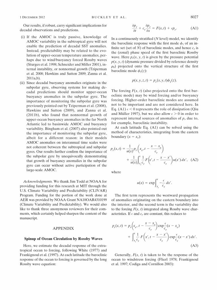
APPENDIX

Spinup of Ocean Circulation by Rossby Waves

Here, we estimate the decadal response of the extra-

tropical ocean to forcing, following White (1977) and

Frankignoul et al. (1997). At each latitude the baroclinic

response of the ocean to forcing is governed by the long

Rossby wave equation:

›pr

›t1 cr

›pr

›x5 F(x, t) 1 �pr. (A1)

In a continuously stratified (N level) model, we identify

the baroclinic response with the first mode f1 of an in-

finite set (set of N) of baroclinic modes, and hence cr is

the (zonal) phase speed of the first baroclinic Rossby

wave. Here pr(x, y, t) is given by the pressure potential

p(x, y, t) (dynamic pressure divided by reference density

r0) projected onto the vertical structure of the first

baroclinic mode f1(z):

p(x, y, z, t) 5 pr(x, y, t)f1(z).

The forcing F(x, t) (also projected onto the first bar-

oclinic mode) may be wind forcing and/or buoyancy

forcing. Higher-order baroclinic modes are assumed

not to be important and are not considered here. In

Eq. (A1) � , 0 represents the role of dissipation (Qiu

and Muller 1997), but we also allow � . 0 in order to

represent internal sources of anomalies of pr due to,

for example, baroclinic instability.

At each latitude Eq. (A1) can be solved using the

method of characteristics, integrating from the eastern

boundary (x 5 xe):

pr(x, t) 51

u(x)pr xe, t 2

x 2 xe

cr

� �

11

u(x)

ðx

xe

1

cr

F x9, t 2x 2 x9

cr

� �u(x9) dx9, (A2)

where

u(x) 5 exp

ðx

xe

2�

cr

dx9.

The first term represents the westward propagation

of anomalies originating on the eastern boundary into

the interior, and the second term is the variability due

to the forcing F(x, t) integrated along Rossby wave char-

acteristics. If � and cr are constant, this reduces to

pr(x, t) 5 pr xe, t 2x 2 xe

cr

� �exp

�

cr

(x 2 xe)

1

ðx

xe

1

cr

F x9, t 2x 2 x9

cr

� �exp

�

cr

(x 2 x9) dx9.

(A3)

Generally, F(x, t) is taken to be the response of the

ocean to windstress forcing (Flierl 1978; Frankignoul

et al. 1997; Codiga and Cornillon 2003):

1 DECEMBER 2012 B U C K L E Y E T A L . 8027

F(x, t) 5 2f 2

hf1(0)R2

bcwe, (A4)

where f is the Coriolis parameter, h is the ocean depth,

and Rbc is the deformation radius. The Ekman velocity

we is given by

we 51

ro

curlzt

f

� �,

where t is the wind stress.

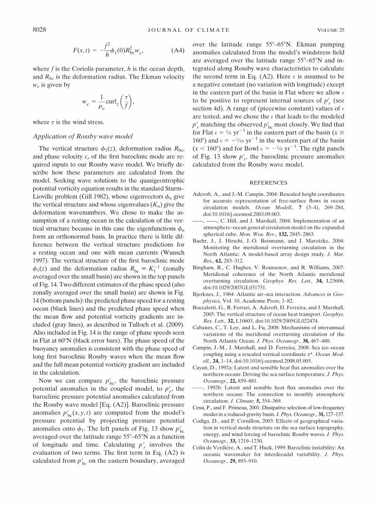
Application of Rossby wave model

The vertical structure f1(z), deformation radius Rbc,

and phase velocity cr of the first baroclinic mode are re-

quired inputs to our Rossby wave model. We briefly de-

scribe how these parameters are calculated from the

model. Seeking wave solutions to the quasigeostrophic

potential vorticity equation results in the standard Sturm–

Lioville problem (Gill 1982), whose eigenvectors fn give

the vertical structure and whose eigenvalues (Kn) give the

deformation wavenumbers. We chose to make the as-

sumption of a resting ocean in the calculation of the ver-

tical structure because in this case the eigenfunctions fn

form an orthonormal basis. In practice there is little dif-

ference between the vertical structure predictions for

a resting ocean and one with mean currents (Wunsch

1997). The vertical structure of the first baroclinic mode

f1(z) and the deformation radius Rbc

[ K211 (zonally

averaged over the small basin) are shown in the top panels

of Fig. 14. Two different estimates of the phase speed (also

zonally averaged over the small basin) are shown in Fig.

14 (bottom panels): the predicted phase speed for a resting

ocean (black lines) and the predicted phase speed when

the mean flow and potential vorticity gradients are in-

cluded (gray lines), as described in Tulloch et al. (2009).

Also included in Fig. 14 is the range of phase speeds seen

in Flat at 608N (black error bars). The phase speed of the

buoyancy anomalies is consistent with the phase speed of

long first baroclinic Rossby waves when the mean flow

and the full mean potential vorticity gradient are included

in the calculation.

Now we can compare p9bc, the baroclinic pressure

potential anomalies in the coupled model, to p9r, the

baroclinic pressure potential anomalies calculated from

the Rossby wave model [Eq. (A2)]. Baroclinic pressure

anomalies p9bc

(x, y, t) are computed from the model’s

pressure potential by projecting pressure potential

anomalies onto f1. The left panels of Fig. 13 show p9bc

averaged over the latitude range 558–658N as a function

of longitude and time. Calculating p9r involves the

evaluation of two terms. The first term in Eq. (A2) is

calculated from p9bc

on the eastern boundary, averaged

over the latitude range 558–658N. Ekman pumping

anomalies calculated from the model’s windstress field

are averaged over the latitude range 558–658N and in-

tegrated along Rossby wave characteristics to calculate

the second term in Eq. (A2). Here � is assumed to be

a negative constant (no variation with longitude) except

in the eastern part of the basin in Flat where we allow �

to be positive to represent internal sources of p9r (see

section 4d). A range of (piecewise constant) values of �

are tested, and we chose the � that leads to the modeled

p9r

matching the observed p9bc

most closely. We find that

for Flat � 5 1/6 yr21 in the eastern part of the basin (x $

1608) and � 5 21/10 yr21 in the western part of the basin

(x , 1608) and for Bowl � 5 21/8 yr21. The right panels

of Fig. 13 show p9r, the baroclinic pressure anomalies

calculated from the Rossby wave model.

REFERENCES

Adcroft, A., and J.-M. Campin, 2004: Rescaled height coordinates

for accurate representation of free-surface flows in ocean

circulation models. Ocean Modell., 7 (3–4), 269–284,

doi:10.1016/j.ocemod.2003.09.003.

——, ——, C. Hill, and J. Marshall, 2004: Implementation of an

atmosphere–ocean general circulation model on the expanded

spherical cube. Mon. Wea. Rev., 132, 2845–2863.

Baehr, J., J. Hirschi, J.-O. Beismann, and J. Marotzke, 2004:

Monitoring the meridional overturning circulation in the

North Atlantic: A model-based array design study. J. Mar.

Res., 62, 283–312.

Bingham, R., C. Hughes, V. Roussenov, and R. Williams, 2007:

Meridional coherence of the North Atlantic meridional

overturning circulation. Geophys. Res. Lett., 34, L23606,

doi:10.1029/2007GL031731.

Bjerknes, J., 1964: Atlantic air–sea interaction. Advances in Geo-

physics, Vol. 10, Academic Press, 1–82.

Boccaletti, G., R. Ferrari, A. Adcroft, D. Ferreira, and J. Marshall,

2005: The vertical structure of ocean heat transport. Geophys.

Res. Lett., 32, L10603, doi:10.1029/2005GL022474.

Cabanes, C., T. Lee, and L. Fu, 2008: Mechanisms of interannual

variations of the meridional overturning circulation of the

North Atlantic Ocean. J. Phys. Oceanogr., 38, 467–480.

Campin, J.-M., J. Marshall, and D. Ferreira, 2008: Sea ice–ocean

coupling using a rescaled vertical coordinate z*. Ocean Mod-

ell., 24, 1–14, doi:10.1016/j.ocemod.2008.05.005.

Cayan, D., 1992a: Latent and sensible heat flux anomalies over the

northern oceans: Driving the sea surface temperature. J. Phys.

Oceanogr., 22, 859–881.

——, 1992b: Latent and sensible heat flux anomalies over the

northern oceans: The connection to monthly atmospheric

circulation. J. Climate, 5, 354–369.

Cessi, P., and F. Primeau, 2001: Dissipative selection of low-frequency

modes in a reduced-gravity basin. J. Phys. Oceanogr., 31, 127–137.

Codiga, D., and P. Cornillon, 2003: Effects of geographical varia-

tion in vertical mode structure on the sea surface topography,

energy, and wind forcing of baroclinic Rossby waves. J. Phys.

Oceanogr., 33, 1219–1230.

Colin de Verdiere, A., and T. Huck, 1999: Baroclinic instability: An

oceanic wavemaker for interdecadal variability. J. Phys.

Oceanogr., 29, 893–910.

8028 J O U R N A L O F C L I M A T E VOLUME 25

Cunningham, S., and Coauthors, 2007: Temporal variability of the

Atlantic meridional overturning circulation at 26.58N. Science,

317, 935–937.

Curry, R. G., M. S. McCartney, and T. M. Joyce, 1998: Oceanic

transport of subpolar climate signals to mid-depth subtropical

waters. Nature, 391, 575–577.

Danabasoglu, G., 2008: On multidecadal variability of the Atlantic

meridional overturning circulation in the Community Climate

System Model, version 3. J. Climate, 21, 5524–5544.

Delworth, T., and M. Mann, 2000: Observed and simulated multi-

decadal variability in the Northern Hemisphere. Climate Dyn.,

16, 661–676.

——, S. Manabe, and R. Stouffer, 1993: Interdecadal variations in

the thermohaline circulation in a coupled ocean–atmosphere

model. J. Climate, 6, 1993–2011.

Deser, C., and M. L. Blackmon, 1993: Surface climate variations

over the North Atlantic Ocean during winter: 1900–1989.

J. Climate, 6, 1743–1753.

Deshayes, J., and C. Frankignoul, 2005: Spectral characteristics of

the response of the meridional overturning circulation to

deep-water formation. J. Phys. Oceanogr., 35, 1813–1825.

Dong, B., and R. Sutton, 2001: The dominant mechanisms of var-

iability in Atlantic Ocean heat transport in a coupled ocean–

atmospheric GCM. Geophys. Res. Lett., 28, 2445–2448.

——, and ——, 2003: Variability of Atlantic Ocean heat transport

and its effects on the atmosphere. Ann. Geophys., 46, 87–97.

Dong, S., and K. A. Kelly, 2004: Heat budget in the Gulf Stream

region: The importance of heat storage and advection. J. Phys.

Oceanogr., 34, 1214–1231.

——, S. L. Hautala, and K. A. Kelly, 2007: Interannual variations in

upper-ocean heat content and heat transport convergence in

the western North Atlantic. J. Phys. Oceanogr., 37, 2682–2697.

Ferrari, R., and D. Ferreira, 2011: What processes drive the ocean

heat transport? Ocean Modell., 38 (3–4), 171–186, doi:10.1016/

j.ocemod.2011.02.013.

Ferreira, D., J. Marshall, and J.-M. Campin, 2010: Localization of

deep-water formation: Role of atmospheric moisture trans-

port and geometrical constraints on ocean circulation. J. Cli-

mate, 23, 1456–1476.

Flierl, G. R., 1978: Models of vertical structure and the calibration

of two-layer models. Dyn. Atmos. Oceans, 2, 341–381,

doi:10.1016/0377-0265(78)90002-7.

Frankcombe, L. M., and H. A. Dijkstra, 2009: Coherent multi-

decadal variability in North Atlantic sea level. Geophys. Res.

Lett., 36, L15604, doi:10.1029/2009GL039455.

Frankignoul, C., P. Muller, and E. Zorita, 1997: A simple model of

the decadal response of the ocean to stochastic wind forcing.

J. Phys. Oceanogr., 27, 1533–1546.

——, A. Czaja, and B. L’Heveder, 1998: Air–sea feedback in the

North Atlantic and surface boundary conditions for ocean

models. J. Climate, 11, 2310–2324.

Fu, L., and B. Qui, 2002: Low-frequency variability of the North

Pacific Ocean the roles of boundary- and wind-driven baro-

clinic rossby waves. J. Geophys. Res., 107 (C12), 3220,

doi:10.1029/2001JC001131.

Ganachaud, A., and C. Wunsch, 2003: Large-scale ocean heat and

freshwater transports during the World Ocean Circulation

Experiment. J. Climate, 16, 696–705.

Gent, P. R., and J. C. McWilliams, 1990: Isopycnal mixing in ocean

circulation models. J. Phys. Oceanogr., 20, 150–155.

Gill, A., 1982: Atmosphere–Ocean Dynamics. Academic Press, 662 pp.

Grist, J., and Coauthors, 2010: The roles of surface heat flux and

ocean heat transport convergence in determining Atlantic

Ocean temperature variability. Ocean Dyn., 60, 771–790,

doi:10.1007/s10236-010-0292-4.

Hasselman, K., 1976: Stochastic climate models. Part I: Theory.

Tellus, 28, 289–305.

Hawkins, E., and R. Sutton, 2009: Decadal predictability of the

Atlantic Ocean in a coupled GCM: Forecast skill and optimal

perturbations using linear inverse modeling. J. Climate, 22,

3960–3978.

Hirschi, J., and J. Marotzke, 2007: Reconstructing the meridional

overturning circulation from boundary densities and the zonal

wind stress. J. Phys. Oceanogr., 37, 743–763, doi:10.1175/

JPO3019.1.

——, P. Killworth, and J. Blundel, 2007: Subannual, seasonal, and

interannual variability of the North Atlantic meridional

overturning circulation. J. Phys. Oceanogr., 37, 1246–1265.

Hristova, H. G., J. Pedlosky, and M. A. Spall, 2008: Radiating in-

stability of a meridional boundary current. J. Phys. Oceanogr.,

38, 2294–2307.

Johns, W. E., and Coauthors, 2010: Continuous, array-based esti-

mates of Atlantic Ocean heat transport at 26.58N. J. Climate,

24, 2429–2449.

Johnson, H. L., and D. P. Marshall, 2002a: A theory for the durface

Atlantic response to thermohaline variability. J. Phys. Oce-

anogr., 32, 1121–1132.

——, and ——, 2002b: Localization of abrupt change in the North

Atlantic thermohaline circulation. Geophys. Res. Lett., 29,

1083, doi:10.1029/2001GL014140.

Kanzow, T., U. Send, W. Zenk, A. Chave, and M. Rhein, 2006:

Monitoring the integrated deep meridional flow in the tropical

North Atlantic: Long-term performance of a geostrophic ar-

ray. Deep-Sea Res. I, 53, 528–546.

Kawase, M., 1987: Establishment of deep ocean circulation driven

by deep-water production. J. Phys. Oceanogr., 17, 2294–2317.

Klinger, B., J. Marshall, and U. Send, 1996: Representation of

convective plumes by vertical adjustment. J. Geophys. Res.,

101 (C8), 18 175–18 182.

Knight, J., R. Allan, C. Follard, and M. Vellinga, 2005: A signature

of persistent natural thermohaline circulation cycles in ob-

served climate. Geophys. Res. Lett., 32, L20708, doi:10.1029/

2005GL024233.

Kushnir, Y., 1994: Interdecadal variations in North Atlantic sea

surface temperatures and associated atmospheric conditions.

J. Climate, 9, 1208–1220.

Kwon, Y.-O., M. Alexander, N. Bond, C. Frankignoul, H. Nakamura,

B. Qiu, and L. A. Thompson, 2010: Role of the Gulf Stream

and Kuroshio–Oyashio systems in large-scale atmosphere–

ocean interaction: A review. J. Climate, 23, 3249–3281.

Lee, T., and J. Marotzke, 1998: Seasonal cycles of meridional

overturning and heat transport of the Indian Ocean. J. Phys.

Oceanogr., 28, 923–943.

Lozier, M. S., 2010: Deconstructing the conveyor belt. Science, 328,

1507–1511, doi:10.1126/science.1189250.

Mann, M., J. Park, and R. Bradley, 1995: Global interdecadal and

century-scale oscillations during the past five centuries. Na-

ture, 378, 266–270.

——, R. Bradley, and M. Hughes, 1998: Global-scale temperature

patterns and climate forcing over the past six centuries. Na-

ture, 392, 779–787.

Marotzke, J., and B. A. Klinger, 2000: The dynamics of equatorially

asymmetric thermohaline circulations. J. Phys. Oceanogr., 30,

955–970.

Marshall, J., A. Adcroft, C. Hill, L. Perelman, and C. Heisey, 1997:

A finite-volume, incompressible Navier Stokes model for

1 DECEMBER 2012 B U C K L E Y E T A L . 8029

studies of the ocean on parallel computers. J. Geophys. Res.,

102 (C2), 5753–5766.

Molteni, F., 2003: Atmospheric simulations using a GCM with

simplified physical parameterizations. I: Model climatology

and variability in multidecadal experiments. Climate Dyn., 20,

175–191.

Msadek, R., and C. Frankignoul, 2009: Atlantic multidecadal

oceanic variability and its influence on the atmosphere in

a climate model. Climate Dyn., 33, 45–62.

Pena-Molino, B., T. Joyce, and J. Toole, 2011: Recent changes in

the Labrador Sea Water within the deep western boundary

current southeast of Cape Cod. Deep-Sea Res. I, 58, 1019–

1030.

Qiu, B., 2002: Large-scale variability in the midlatitude subtropical

and subpolar ocean: Observations and causes. J. Phys. Oce-

anogr., 32, 353–375.

——, and P. Muller, 1997: Propagation and decay of forced and free

baroclinic Rossby waves in off-equatorial oceans. J. Phys.

Oceanogr., 27, 2405–2417.

——, and S. Chen, 2006: Decadal variability in the large-scale sea

surface height field of the South Pacific Ocean: Observations

and causes. J. Phys. Oceanogr., 36, 1751–1762.

Redi, M. H., 1982: Oceanic isopycnal mixing by coordinate rota-

tion. J. Phys. Oceanogr., 12, 1154–1158.

Ripa, P., 1978: Normal Rossby basin modes of a closed basin with

topography. J. Geophys. Res., 83 (C4), 1947–1957.

Schneider, N., and A. Miller, 2001: Predicting western North Pa-

cific Ocean climate. J. Climate, 14, 3997–4002.

Seager, R., Y. Kushnir, P. Chang, N. Naik, J. Miller, and W. Hazeleger,

2000: Causes of Atlantic Ocean climate variability between

1958 and 1998. J. Climate, 13, 2845–2862.

Shaffrey, L., and R. Sutton, 2006: Bjerknes compensation and

the decadal variability of the energy transports in a cou-

pled climate model. J. Climate, 19, 1167–1181, doi:10.1175/

JCLI3652.1.

Sime, L., D. Stevens, K. Heywood, and K. Oliver, 2006: A de-

composition of the Atlantic meridional overturning. J. Phys.

Oceanogr., 36, 2253–2270.

Sirven, J., C. Frankignoul, D. DeCoetlogon, and V. Tailandier,

2002: Spectrum of wind-driven baroclinic fluctuations of the

ocean in the midlatitudes. J. Phys. Oceanogr., 32, 2405–2417.

Spence, P., O. Saenko, W. Sijp, and M. England, 2012: The role of

bottom pressure torques in the interior pathways of North

Atlantic Deep Water. J. Phys. Oceanogr., 42, 110–125.

Spydell, M., and P. Cessi, 2003: Baroclinic modes in a two-layer

basin. J. Phys. Oceanogr., 33, 610–622.

Sturges, W., and B. Hong, 1995: Wind forcing of the Atlantic

thermocline along 328N at low frequency. J. Phys. Oceanogr.,

25, 1706–1715.

——, ——, and A. Clark, 1998: Decadal wind forcing of the North

Atlantic subtropical gyre. J. Phys. Oceanogr., 28, 659–698.

Talley, L., 2003: Shallow, intermediate, and deep overturning

components of the global heat budget. J. Phys. Oceanogr., 33,

530–560.

te Raa, L. A., and H. A. Dijkstra, 2002: Instability of the thermo-

haline ocean circulation on interdecadal timescales. J. Phys.

Oceanogr., 32, 138–160.

——, J. Gerrits, and H. A. Dijkstra, 2004: Identification of the

mechanism of interdecadal variability in the North Atlantic

Ocean. J. Phys. Oceanogr., 34, 2792–2807.

Ting, M., Y. Kushnir, R. Seager, and C. Li, 2009: Forced and in-

ternal twentieth-century SST trends in the North Atlantic.

J. Climate, 22, 1469–1481.

Toole, J., R. Curry, T. Joyce, M. McCartney, and B. Pena-Molino, 2011:

Transport of the North Atlantic deep western boundary current

about 398N, 708W: 2004–2008. Deep-Sea Res. II, 58, 1768–1780.

Trenberth, K. E., and J. M. Caron, 2001: Estimates of meridional

atmosphere and ocean heat transports. J. Climate, 14, 3433–3443.

Tulloch, R., and J. Marshall, 2012: Exploring mechanisms of vari-

ability and predictability of Atlantic meridional overturning

circulation in two coupled climate models. J. Climate, 25,

4067–4080.

——, ——, and K. S. Smith, 2009: Interpretation of the propagation

of surface altimetric observations in terms of planetary waves

and gesotrophic turbulence. J. Geophys. Res., 114, C02005,

doi:10.1029/2008JC005055.

Tziperman, E., L. Zanna, and C. Penland, 2008: Nonnormal ther-

mohaline circulation dynamics in a coupled ocean–atmosphere

GCM. J. Phys. Oceanogr., 38, 588–604.

Walker, A., and J. Pedlosky, 2002: Instability of meridional baro-

clinic currents. J. Phys. Oceanogr., 32, 1075–1093.

Wang, J., 2011: Instabilities of an eastern boundary current with

and without large-scale flow influence. Ph.D. thesis, Massa-

chusetts Institute of Technology, 227 pp.

White, W., 1977: Annual forcing of baroclinic long waves in the

tropical North Pacific Ocean. J. Phys. Oceanogr., 7, 50–61.

Winton, M., 1997: The damping effect of bottom topography on

internal decadal-scale oscillations of the thermohaline circu-

lation. J. Phys. Oceanogr., 27, 203–208.

Wunsch, C., 1997: The vertical partition of oceanic horizontal ki-

netic energy. J. Phys. Oceanogr., 27, 1770–1794.

Zanna, L., P. Heimbach, A. Moore, and E. Tziperman, 2011a:

Upper ocean singular vectors of the North Atlantic climate

with implications for linear predictability and variability.

Quart. J. Roy. Meteor. Soc., 138, 500–513, doi:10.1002/qj.937.

——, ——, ——, and ——, 2011b: Optimal excitation of in-

terannual atlantic meridional overturning circulation vari-

ability. J. Climate, 24, 413–427.

Zhang, R., 2008: Coherent surface-subsurface fingerprint of the

Atlantic meridional overturning circulation. Geophys. Res.

Lett., 35, L20705, doi:10.1029/2008GL035463.

——, 2010: Latitudinal dependence of Atlantic Meridional over-

turning circulation (AMOC) variations. Geophys. Res. Lett.,

37, L16703, doi:10.1029/2010GL044474.

——, T. Delworth, and I. Held, 2007: Can the Atlantic Ocean drive

the observed mulidecadal variability in the Northern Hemi-

sphere mean temperature? Geophys. Res. Lett., 34, L02709,

doi:10.1029/2006GL028683.

8030 J O U R N A L O F C L I M A T E VOLUME 25