On the risk spillover across the oil market, financial …meea.sites.luc.edu/volume18/pdfs/212-On the Risk.pdfmodel, and (2) to discern how major global events affect the volatility

Topics in Middle Eastern and African Economies Vol. 18, Issue No. 2, September 2016

211

On the risk spillover across the oil market, financial markets, and the oil-related

CDS sectors: A Volatility impulse response approach

Mehmet Balcılar1, Shawkat Hammoudeh2, Elif Akay Toparlı3

Abstract In contrast to previous CDS literature, this study focuses on the magnitude of volatility transmission and the risk spillover mechanism across the oil market, financial market risks, and the oil-related Credit Default Swap (CDS) sectors. Our dataset includes futures prices of West Texas Intermediate (WTI) in addition to seven different measures of markets and credit risks. Four of the vast risk measures are the oil-related sector CDSs for auto, chemicals, natural gas, and utility sector CDSs. Two measures of the financial market risk are further included in the study, which include the one-month expected equity volatility measured by the volatility index (VIX) and the one-month bond option volatility estimate (MOVE) or swaption move expected volatility (SMOVE). The daily dataset covers the period from January 6, 2004 to February 2, 2016. The volatility transmission mechanism across the oil and financial markets and CDS sectors is examined, using the volatility impulse responses. In addition to showing the magnitude of the volatility transmission, the volatility impulse responses have the advantage of providing valuable information on the speed of risk transmission among different markets. The shape and sign of the volatility impulse responses also provide significant information on the transmission mechanism. We evaluate the risk transmission due to several recent crisis shocks. The results show complicated transmission mechanisms that spread over long periods. Keywords: Risk; Sectoral CDS; VIX; SMOVE; MOVE; Volatility impulse response JEL Classification: C13, C22, G1, G12, Q40

1 Eastern Mediterranean University, Famagusta, T. R. North Cyprus, University of Pretoria, Pretoria 0002, South Africa; AND , IPAG Business School, Paris, France, e-mail: [email protected] 2, Drexel University, Philadelphia, PA 19104, USA. IPAG, IPAG Business School, Paris, France 3 Department of Economics, Eastern Mediterranean University, Famagusta, T. R. North Cyprus, [email protected]


212

1. Introduction

Oil can be considered as the most prominent and volatile commodity in the world economy and

financial markets. Oil and oil-based products are not only used directly as raw materials by many

economic sectors but also are used in many service sectors and traded on exchange markets. Because

of high and growing demand (and constraints on supply), oil has become very valuable and volatile.

Therefore, any fluctuations in oil prices have significant worldwide and regional effects on the world’s

economies. Many factors including supply-demand, global economic developments and political

issues have profound effects on oil prices which are connected to other markets. The study of the

transmission of risk shocks across oil and financial markets has recently gained more attention from

researchers, oil industry and policymakers, particularly in the wake of recent major global crises. The

Asian Financial Crisis in 1997, the Iraq War in 2003 the US subprime crisis at the end of 2007, the

European sovereign debt crisis since the end of 2009 have been the catalysts for more research on

volatility and the risk transmission mechanism among oil and financial markets. After Iraq War, WTI

(West Texas Intermediate) future price declined to $31.21 on February 6, 2004.

The WTI oil price of oil was $146.12/barrel in July 2008, then nose-dived to $39.72/barrel in

the middle of February 2009, as a result of the 2008 global economic crisis. Recently, it dropped more

than 70% since June 2014. It reached $29.694 in January 2016 because of the supply glut. The ten year

nominal bond rates in the United States have declined from 275 basis points to 225 basis points in

October 2015 to about 180 basis points in January 2016. The financial market also decline by half over

the same period.

The major events that have affected the oil and financial markets have associated shocks also

have a negative effect on the credit default swap (CDS) spreads which reflect the health of the economy

and increases and decreases in the risk level of oil-related sectors. Due to mortgage crisis in 2007, the

CDS market reached a record level of $60 trillion up from two trillion dollars in 2002. This market in

4 http://www.bloomberg.com/quote/CL1:COM


213

December 2010 was 29.9 trillion and finished the 2012 with the value of 25.1 trillion according to a

survey of ISDA5. The Energy producer-weighted CDS risk is now over 2009 levels. Defaults are rising

across smaller oil and gas producers and risks are rising for larger ones as well.

The fear index, CBOE volatility index (VIX) which measures one-month expected equity

volatility of the S&P 500. The expected risk in the bond market is represented by the Merrill Lynch

Option Volatility Estimate (MOVE) Index and the expected risk in the swap market is measured by

the Swaption Move Expected Volatility (SMOVE) index. In other words, VIX is correlated with the

equity market, MOVE is with US Treasury securities market and SMOVE can be considered as a kind

of VIX for US non-Treasury in swaption markets.

The daily closing future prices of WTI and seven different measures of risk are used in the

analysis of this paper. Four of the vast risk measures are oil and oil-related sector CDSs, which include

auto (AUTO), chemicals (CHE), natural gas (OILGAS), and utility (UTIL) sectors. Others are the one-

month expected equity volatility measured by VIX, one-month MOVE and SMOVE indices. The

seven variables investigated in this paper were not only used as risk measurement tools but also used

to represent the volatilities in different markets and sectors.

This study has the following objectives: (1) to examine the volatility transmission mechanism

across the oil, oil-related CDS sectors and financial markets, using a multivariate conditional volatility

model, and (2) to discern how major global events affect the volatility of the oil, oil-related and CDS

markets by employing the newly introduced volatility impulse response function analysis. To examine

the risk spillover mechanism within and across the oil market, financial market, and the oil related

CDS sectors; eight variables (WTI, four oil and oil-related sector CDSs, VIX, MOVE and SMOVE)

were employed in the multivariate conditional volatility model, known as BEKK model, by Engle and

Kroner, 1995. In addition, the Volatility Impulse Response Function (VIRF) model developed by

5http://www2.isda.org/attachment/NTY4MQ==/ISDA%20YearEnd%202012%20Market%20Analysis%20FINAL.pdf


214

Hafner and Herwartz (2006) is applied to our dataset to assess the magnitude of the volatility

transmission. We evaluate the risk transmission on oil and oil-related market volatilities due to

following events: US Mortgage Crisis; Lehman Brothers Bankruptcy on September 17, 2008; the

Greece Debt Crisis on December 8, 2009; the Fear of Greece's Default on April 23, 2010; the Egyptian

Political Unrest (Second Revolution) on May 27, 2011; the European Sovereign Debt Crisis on August

18, 2011; and the US Government Shutdown on September 30, 2013. The volatility impulse responses

have the advantage of providing valuable information on the speed of risk transmission, and the shape

and sign of the volatility impulse responses also provide significant information on the transmission

mechanism. Therefore, the study of volatility transmissions within and across the oil and oil-related

sectors and also determining the dynamic relationships between the oil prices, oil-related CDS sector

indices, VIX, MOVE/SMOVE are valuable to oil companies, market investors, creditors of these

sectors, energy regulators and Government for future decisions and actions.

The remainder of this paper is organized as follows. Section 2 presents a brief literature review.

Section 3 describes the data and descriptive statistics. Section 4 presents econometric methodology of

the volatility impulse response function, while Section 5 discusses the empirical results including the

conclusion part and giving some remarks for the future studies.

2. Literature review

2.1. Volatility impulse response function (VIRF) method The Error Shock Methodology named also as Impulse Response Analysis is employed to understand

the effects of a shock on the behavior of time series. Most of the early papers on Impulse Response

Analysis in the literature employed linear equations. The first paper about this concept was written by

Sims, 1980 and improved by Doan et al., 1983. Sims, 1980 studied the analysis of shocks on volatility

in linear models. Sims, 1980 identified the impulse response analysis providing dynamic effects of an

error shock in the system on future economic variables. Single linear equations or Vector


215

Autoregressive (VAR) model were used to show the links between international equity returns. The

initial studies of the international finance on spillover effect were conducted by Eun and Shim, 1989

and Becker et al., 1990. Blanchard and Quah, 1989 investigated the persistence of shocks on linear

multivariate time series. Engle et al., 1990 introduced two important concepts known as “meteor

showers” and “heat waves”. “Meteor showers” showed the transmission of volatility from one market

to another and “heat waves” indicated the increased persistence in market volatility using linear

equations. Koch and Koch, 1991 studied on the regional interdependence by using lead/lag

relationships among eight financial markets. Their findings showed regional interdependence between

markets growing over time and the influence of the Japanese market increases at the expense of the

US market. They focused only on the return series and correlations, in other words, focused only on

interdependence through the mean of the processes.

Linear time series models studied in the past were mainly using basic linear models. However,

Beaudry and Koop, 1993, Potter, 1995, Pesaran and Potter, 1997 demonstrated that linear models are

not adequate for studying on persistence effect of shocks on time series because of symmetry. Since,

it is very difficult to distinguish differences between the effect of shocks occurring in an expansion

period and a recession period in linear models. The early basic models using univariate linear equations

were initially improved by models employing linear multivariate equations, offered by Pesaran et al.,

1993 and Lee and Pesaran, 1993.

Further improvements were also conducted by employing models using nonlinear equations,

which were able to demonstrate more complexities compared to linear models. Two different

definitions of Impulse Response Analysis using nonlinear models were offered by Gallant et al., 1993

and Koop et al., 1996. Gallant et al., 1993 made use of a semi-nonparametric methodology for

nonlinear system in their Impulse Response Analysis. Two concepts were defined: the “baseline” and

the “shocked”. In their paper, the difference between the baseline approach and the shocked was

approved as the conditional moment profile. And this shock should be either observable or estimated.


216

Koop et al., 1996 offered a new method. The difference between mean of the response vector

conditioned on both history and present shock and the mean that only conditioned on history was found

so that a new concept of generalized nonlinear impulse response functions for the conditional

expectation was introduced and named as the Generalized Impulse Response Function (GIRF). Lin,

1997 contributed the idea of Gallant et al., 1993 by filling the gap in the generalized autoregressive

conditional heteroscedasticity (GARCH) literature by tracing the dynamics of the conditional variance

from past squared innovations for the Impulse Response Function. In the paper, the Impulse Response

Function for conditional volatility in GARCH model’s standard error was found. Then, first-order

derivatives of the function and the covariance matrix of the estimated parameters were traced. Monte

Carlo analysis was employed to find the finite sample properties of the standard errors. It was also

concluded that despite the process itself being nonlinear, the conditional variance was linear. In 1990s,

Hamao et al., 1990, Engle and Ng, 1993, Lin et al., 1994, Karolyi, 1995, Koutmos and Booth, 1995

and Booth et al., 1997 traced the effects of shocks over time using Impulse Response Analysis and

investigated whether the volatility was transferred from one market to another. Ewing et al., 2002

studied volatility transmission in energy markets on stock indices of oil and gas companies. Serletis

and Shahmoradi, 2006 examined volatility spillovers between gas and electricity prices in Canada.

Compared to earlier studies, Hafner and Herwartz, 2006 looked at the conditional variance rather

than the conditional mean. According to their paper, it was considered that two news appearing in

different series at the same time are independent. Owing to this assumption of news, it can be assumed

as independent both over time and across the series. Whenever its distribution is not normal, the

method helps to identify shocks. News is claimed as independent and identically distributed in other

words, inherently independent over time. Hafner and Herwartz, 2006 created volatility impulse

response function (VIRF) which is an application of Koop et al., 1996 definition to the multivariate

generalized autoregressive conditional heteroscedasticity (MGARCH) models. The VIRF was used


217

for checking the effects of independent shocks of a market on volatility of another market and also the

persistence of these spillover effects in multivariate nonlinear models.

The effects of central bank decisions on the foreign exchange market volatility were checked for

the effects of independent shocks on volatility through time by ignoring orthogonality and ordering

problems. In order to avoid these problems, Jordan decomposition was applied to retrieve an

independent and realistic shock from the conditionally heteroskedastic error terms. Hafner and

Herwartz, 2006 proved that news is inherently uncorrelated over time because of being a risk source

that is independent and unpredictable which first introduced by Gallant et al., 1993. This assumption

is directive in future studies. Panopoulou and Pantelidis, 2009 investigated the connection between the

US and the rest of the G-7 countries and international information flow between these countries by

using daily financial market return data based on VIRF analysis for 20 years. According to their

findings for post-1995 period, connections between markets were changed significantly, in other

words, interdependence in the volatility of the markets increased. Panopoulou and Pantelidis, 2009

argued that the VIRF method developed by Hafner and Herwartz, 2006 is well suited for the analysis

on volatility spillover. First of all, it helps to show how a shock in one market could affect the other

market’s dynamic adjustment of volatility to another market and the persistence of these spillover

effects. Another reason is that, when shocks occur, VIRF depends on both the state of actual system’s

volatility and the unexpected returns vector. This shows a given shock will not always increase

expected conditional volatility. The asymmetric response of volatility can be negative and positive.

Finally, owing to the application of Jordan decomposition, VIRF approach avoids typical

orthogonalization and also ordering problems which is hardly feasible in the presence of highly

interrelated and at high frequency financial time series. Diebold and Yilmaz, 2009 examined

interdependence between asset returns and/or volatilities by measuring return spillovers and volatility

spillovers.


218

From the early 1990s to the present, daily nominal local-currency financial market indices of

nineteen global equity markets (seven developed financial markets and twelve emerging markets) were

analyzed. According to results, a divergent behavior in the dynamics of return spillovers vs. volatility

spillovers was observed. Spillover intensity was time varying and it was different for returns vs.

volatilities as the nature of the time-variation. Return spillovers had no bursts but increasing trend,

also increasing financial market integration for the last fifteen years. However, volatility spillovers

displayed no trend but clear bursts because of the relevance of crisis. Le Pen and Sévi, 2010 quantified

the effect of shocks on return volatilities in three electricity forward markets: British, Dutch and

German. For the analysis of forward OTC (Over-the-Counter) electricity daily price data, they used

MGARCH model and VIRF methodology. Limited numbers of papers investigated the volatility

spillovers in energy markets. And most of them use the mean of the processes for transmissions than

moments. Grobys, 2010 investigated the cointegration of European financial markets and studied the

volatility spillover effects. A new concept was introduced, the advance of VIRF, to capture the overall

impacts of volatility spillovers from one market on to another market named as Volatility Impulse

Response Density Function (VIRDF). The sample data was divided into two parts: 1990-2000 and

2000-2010. Grobys, 2010 focused on the asset return series and how returns were correlated across

different economies.

The financial markets’ mean processes and a method determining changes concerning second-

order moments over time were investigated in the model consisting of VAR and MGARCH models.

Grobys, 2010 suggested that VIRDF presented a precise estimation of the overall volatility spillover

effects considering within a certain time window since volatility shocks were continuous random

variables. In addition, the probability of shocks was included in this study. Increasing or decreasing

volatility spillover effects could be embraced as the difference of the volatility spillover effects

between different time windows founded by VIRDF. Consequently, according to the findings of

Grobys, 2010, there was an increasing volatility spillover impact among countries. Adams et al., 2015


219

created a state-dependent sensitivity value-at-risk (SDSVaR) model for quantifying risk spillover

among 74 U.S. Real Estate Investment Trusts (REITs). They checked the direction of risk spillover

effects from one REIT to another. For risk spillover size, estimation of the link between geographic

distance and risk spillover was conducted. Therefore, these estimates were not only quantifying the

size but also the direction. Their findings showed that vulnerability to risk in other REITs was

significantly increased by high leverage, size, and market beta by increasing the probability of

contagion during a financial crisis.

2.2. Volatility Impulse Response Function (VIRF) Method using CDS Credit Default Swaps (CDS) index spread is a newly introduced concept; therefore, the number of

studies is very limited. In addition, the limited availability of data on CDS also affects the study of

economic analysis. As far as we know, there is no paper related to CDS especially studying on our

selected shocks in VIRF analyses. The following studies use cross sectional data while analyzing on

CDS spreads (equity and credit markets). Longstaff et al., 2005 examined the difference between

corporate bond-implied CDS spreads and the actual market CDS spreads and found the former being

higher than the latter. Das and Hanouna, 2006 investigated the change between cash/asset market CDS

spread and credit market CDS.

CDS spread was considered as a measure of credit risk in the following papers. Bharath and

Shumway, 2004 is another example on credit risk study. Ericsson et al., 2009 investigated the links

between theory-based determinants of default risk and default swap spreads.

A significant portion of the variation in the data was explained by the theory-based variables.

Berndt et al., 2008 examined the degree of variations in the credit risk premium of CDS spread in

broadcasting and entertainment, health care, oil and gas sectors over time. According to the results,

variations in the credit risk premium were significantly different. Zhang et al., 2009 studied the CDS

premium, the volatility and jump risks of individual firms because of high frequency stock prices. The

jump risk and volatility risk predicted 19% and 48% of the variation in CDS spread levels, respectively.


220

By controlling the internal and external influences, they predicted 6% more variation than before. As

a result, the credit spreads could be explained by the high frequency-based volatility measures.

CDS was examined by time series as in the following studies. Byström, 2006 investigated Dow

Jones iTraxx CDS indices, i.e. indices of CDS securities of the seven sectors (industrials, autos, energy,

technology-media- telecommunications, consumers, senior financials and sub-ordinated financials)

covering the European market. Byström, 2006 found a connection between iTraxx CDS index market

and the financial market. The stock price volatility was highly correlated with CDS spreads and there

was a significant positive autocorrelation in the iTraxx market. Zhu, 2006 showed the high response

of CDS premium to credit conditions by using vector error correction model (VECM) and found a

long-run relationship between credit risk in the corporate bond market and CDS market. Fung et al.,

2008 discovered the links between stock and CDS markets in US and it was shown that the lead/lag

relationships between those markets depended on the credit quality. Forte and Lovreta, 2008 found the

stronger relationship at lower credit quality levels after examining the link between financial market

and company level CDS. Norden and Weber, 2009 was also examined the relation between CDS, bond

and financial markets.

Monthly, weekly and daily lead-lag relationships in VAR models for period from 2000 to 2002

were investigated. According to their findings, stock returns led a change in CDS and bond spread. In

addition, the CDS market was found more sensitive to the financial market than the bond market and

this tendency increased for lower credit quality and larger bond issues. Finally, it was shown that the

CDS market contributed more to price discovery than the bond market and this was stronger for US

firms than for European firms. Becker et al., 2009 evaluated two issues related to volatility index

(VIX). First issue was on how historical jump activity made contribution to the price volatility. The

other issue was to check whether VIX reflected any incremental information to future jump activity.

Their findings showed that VIX carried information about both related to past jump contributions on

total volatility and incremental information relevant to future jumps. It is an important study showing


221

how option markets form volatility forecasts. By using a general VECM representation with a sample

of North American and European firms, Forte and Peña, 2009 studied the dynamic relationship

between financial market implied credit spreads, CDS spreads, and bond spreads. The empirical results

on price discovery indicated the leading role of CDS with respect to bonds. Figuerola-Ferretti and

Paraskevopoulos, (2011) argued the nature of the relation between credit risk and market risk. It was

claimed that there were long-term relationships in VIX and CDS markets for most companies.

Figuerola-Ferretti and Paraskevopoulos, 2011 revealed the cointegration in VIX and iTraxx/CDS

markets. In addition, VIX had a clear lead over the CDS market in the price discovery process. When

there was a temporary mispricing from the long-run equilibrium, CDS could adjust to market risk. Luo

and Zhang, 2012 extended the use of VIX to other maturities. Daily VIX term structure data from 2009

was offered by using a simple two-factor stochastic volatility framework for the VIXs. It was shown

that VIX contained more information than historical volatility. According to the results, both the time

series dynamics of VIXs and the rich cross-sectional shape of the term structure were captured by the

framework. Luo and Zhang, 2012 made analysis on WTI, Dubai and Brent crude oil markets futures

contracts and these market integrations on second moment with VAR-BEKK model. The range of the

daily data was from 2005 to 2011. VIRF analysis revealed two historical shocks; the 2008 Financial

Crisis and the BP Deepwater Horizon oil spill, and also quantified the size and persistence. The

observations showed that Brent and Dubai crude oil markets were highly responsive to market shocks.

The probability of observing a large impact of a shock was also lower while the probability of a smaller

impact was opposite. Only a large shock, which was derived from small probability, was able to show

an increase in expected conditional volatilities.

In contrast to the previous studies, Hammoudeh et al., 2013 focused on variable relationships

at the sector level, not the firm level. Risk transmission and migration among six US measures of credit

and market risk were examined. The data used in the series of analysis were from 2004 to 2011.

However a sub-period of 2009 to 2011 was also used to analyze the effects of shocks in 2007–2008


222

Great Recession. Four oil exploration and production sectors namely the natural gas, utility, chemicals

and auto sectors were investigated. According to the study, there were more long-run equilibrium risk

relationships and short-run causal relationships among the four oil-related CDS spreads, the VIX index

and the swaption expected volatility (SMOVE) index for the full period and the sub-period. In addition,

the four oil-related CDS spreads were responsive to VIX in the short and long-run, whereas none of

the indices were sensitive to SMOVE. The auto sector’s CDS spread was the most error correcting in

the long run and in the short run. It was pioneering in the risk discovery process. Furthermore, the

2007–2008 Great Recession showed “localization” and less migration of credit and market risk in the

oil-related sectors.

Fernandes et al., 2014 examined the time series properties of the daily market VIX from the

Chicago Board Options Exchange (CBOE). According to results, there was a negative relationship

between the VIX and the S&P 500 index returns as well as a positive contemporaneous relationship

with the volume of the S&P 500 index and VIX displayed long-range dependence. In addition, it was

found that VIX tended to decline as the long-run oil price increased, reflecting the high demand from

oil in recent years.

In this paper, we employ VIRF method for MGARCH model introduced by Hafner and

Herwartz, 2006, which enable to examine our data for any unbiased transmission flow patterns. We

focus on sector level for oil and oil related sectors as discussed in Hammoudeh et al., 2013. Focusing

on the sector level is important because of the arising interest of energy regulators, policy-makers and

investors in the energy and energy-related sectors. We use CDS spreads for all 4 sectors; auto (AUTO),

chemicals (CHE), natural gas (OILGAS), utility (UTIL); and indices of VIX, MOVE and SMOVE as

variables. Our daily dataset covers the period from the beginning of January 2004 to February 2016.

We examine the risk spillover mechanism across the oil market, financial market, and the oil related

sectors’ CDSs. Different than Hammoudeh et al., 2013, the volatility transmission mechanism across

the oil and financial markets and sector CDS is examined by using the Volatility Impulse Response


223

Function, having the advantage of providing valuable information on the speed of risk transmission.

The shape and sign of the Volatility Impulse Response also provides significant information on the

transmission mechanism of historical shocks. The effects of six specific events on residuals are

researched. This study enables the migration of risk in the markets and four oil exploration and

production sectors at a time of volatile oil prices.

3. DATA and DESCRIPTIVE STATISTICS

3.1. Data Our data includes the daily closing future prices of West Texas Intermediate (WTI), Credit

Default Swap (CDS) indices for four sectors (AUTO, CHE, OILGAS and UTIL), Volatility Index

(VIX), one-month Merrill Lynch Option Volatility Estimate (MOVE) Index and Swaption Move

Expected Volatility (SMOVE) Index. The daily dataset covers the period from 6 January 2004 to 2

February 2016 for five working days. Prices are quoted in US dollars per barrel and the data is obtained

from Datastream.

CDS is a type of swap insured by the swap seller to remove the risk of non-payment on the

security’s premium and also interest payments at the end of the maturity date of a contract. Therefore,

swap buyer makes payments to seller until the maturity date of a contract. In other words, the credit

exposure of fixed income products is transferred between two parties, i.e. buyer of the swap and the

seller. The risk is transferred in the way of paying CDS pre mia determined by current estimated

calculations depending on the country risk. CDS spread is smaller for developed countries compared

to developing ones. In our study, CDS spread represents the risk, fear, present and future economic

health of four oil and oil-related sectors including auto, chemicals, natural gas, and utility sectors. The

one-month expected equity volatility of the S&P 500 index measured by the VIX. Known also as

uncertainty or fear index, VIX is used to understand whether there is fear or enthusiasm on the asset

and gives an idea about the risk level by showing the volatility of the price of an asset. When the price


224

of a good increases, VIX also increases meaning that the risk becomes higher. The value of VIX greater

than 30% is a sign of devolving in the course of the economy and leads to an increase in the risk

perception of investors expecting the value of the S&P 500 index fluctuate in next 30 days. However,

the value of 20% in VIX represents opposite that diminution in the risk perception and positive future

expectations for the course of economy. MOVE index represents expected risk in the bond market and

is a yield curve weighted index of the normalized implied volatility on one-month US Treasury

maturities, which are weighted on the 2, 5, 10, and 30 years contracts. MOVE is 40% on the 10-year

Treasury and 20% on the other Treasury options. VIX is correlated with equity; MOVE is with US

Treasury options. On the other hand, expected risk in the swap market is measured by the SMOVE

index. It is a kind of VIX for US non-Treasury in swaption markets and measures volatility on one to

ten years US non-Treasury options depending on inflation, deflation, massive rolling of Government

debts and interest rate movements. MOVE/SMOVE movements are dramatic and responses are in

opposite compared to VIX.

We employ the first logarithmic differences for all eight variables in time series analysis. All

daily prices converted into a daily nominal return series:

𝑋𝑋 = ln�(𝑋𝑋𝑡𝑡 𝑋𝑋𝑡𝑡−1⁄ )� for t=1,2,…,T Eq.1

where 𝑋𝑋 𝑖𝑖𝑖𝑖 the returns for all variables used in the study, 𝑋𝑋𝑡𝑡is the current level at time t and 𝑋𝑋𝑡𝑡−1is

previous day’s value.


225

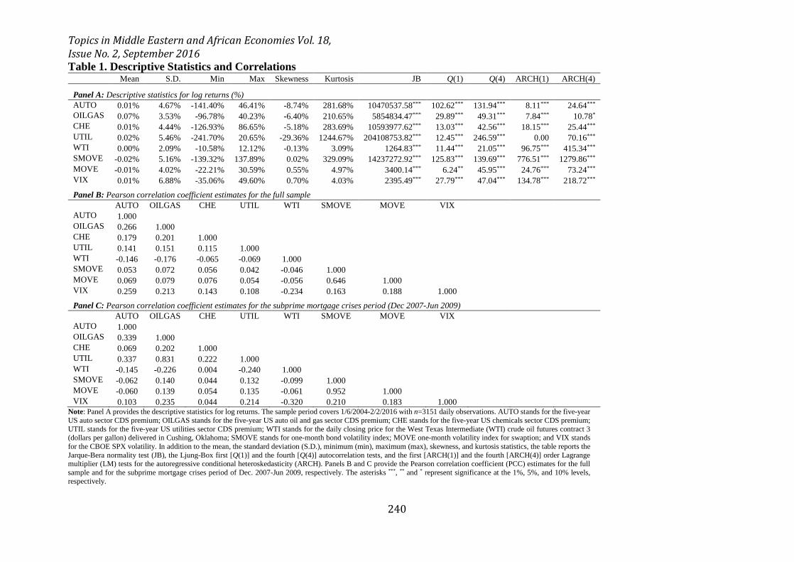
3.2. Descriptive Statistics and Correlations

The descriptive statistics are given in Table 1 (Panel A, B and C). All variables are in first natural

logarithmic differences. For full period, the number of observations is 3151 and same for all the series.

The mean of all the variables are very close to zero. The standard deviation, measure of volatility,

varies between 2.09-6.88%. The most volatile measure is VIX, despite the low peak-to-valley

difference, i.e. the range of the data obtained from Min and Max. The lowest volatility observed for

WTI. Considering the peak-to-valley difference, UTIL and SMOVE have the highest, correlating with

high standard deviations. MOVE, SMOVE and VIX return series are skewed to the right, i.e. positive

skewed and the data for the rest of the variables show negative skewness. The skewness values of

WTI, SMOVE, MOVE and VIX are very close to zero. This means that the distributions of the data

for these variables are close to normal distribution. The kurtosis values of oil and oil-related sectors

are very high particularly UTIL. Therefore, it can be concluded that there are high leptokurtic

distributions for oil and oil-related sectors. SMOVE index also has high value on kurtosis.

All variables were checked by Jarque and Bera, 1980 (JB) Langrange multiplier test whether

series show normal distribution or not. According to the test results, all variables rejected the null

hypothesis of not having normal distribution with zero probabilities of the test, which could be also

observed from the skewness and kurtosis values. Because of the finding, we employed Student’s t-

distribution for our analyses. The Box–Pierce Portmanteau Q statistics for lagged 1 and lagged 4 orders

were also calculated. All residual series were found to be independently distributed at 5% significance

level. According to statistical results presented in Table 1 Panel A, it was concluded that

implementation of Student’s t distribution to the series’ error terms were more suitable instead of

normal distribution.

All residuals were tested by the first [ARCH(1)] and the fourth [ARCH(4)] order Lagrange

multiplier (LM) tests for the autoregressive conditional heteroskedasticity (ARCH). The tests rejected


226

the homoscedasticity hypothesis at the significance level of 1% up to 4 lagged orders except UTIL in

1 lagged order.

For full period, the sample was checked for the Pearson Correlation Coefficient (PCC). As can be

seen in Table 1 Panel B, MOVE is highly interdependent with SMOVE compared to other PCCs, as

observed by Hammoudeh et al., 2013. Table 1 Panel C represents the PCC estimates for the subprime

mortgage crisis period. The correlation coefficient of MOVE and SMOVE is very close to 1 suggesting

a high interdependency as found for the full period. However, UTIL and OILGAS have also high PCC,

which is not observed for the full period. It can be concluded from Table 1 that the correlations between

WTI and risk measures are low excluding the correlation between MOVE-SMOVE for both periods.

Therefore, we can conclude that risk measures used in this study for the full period give information

about different risks.

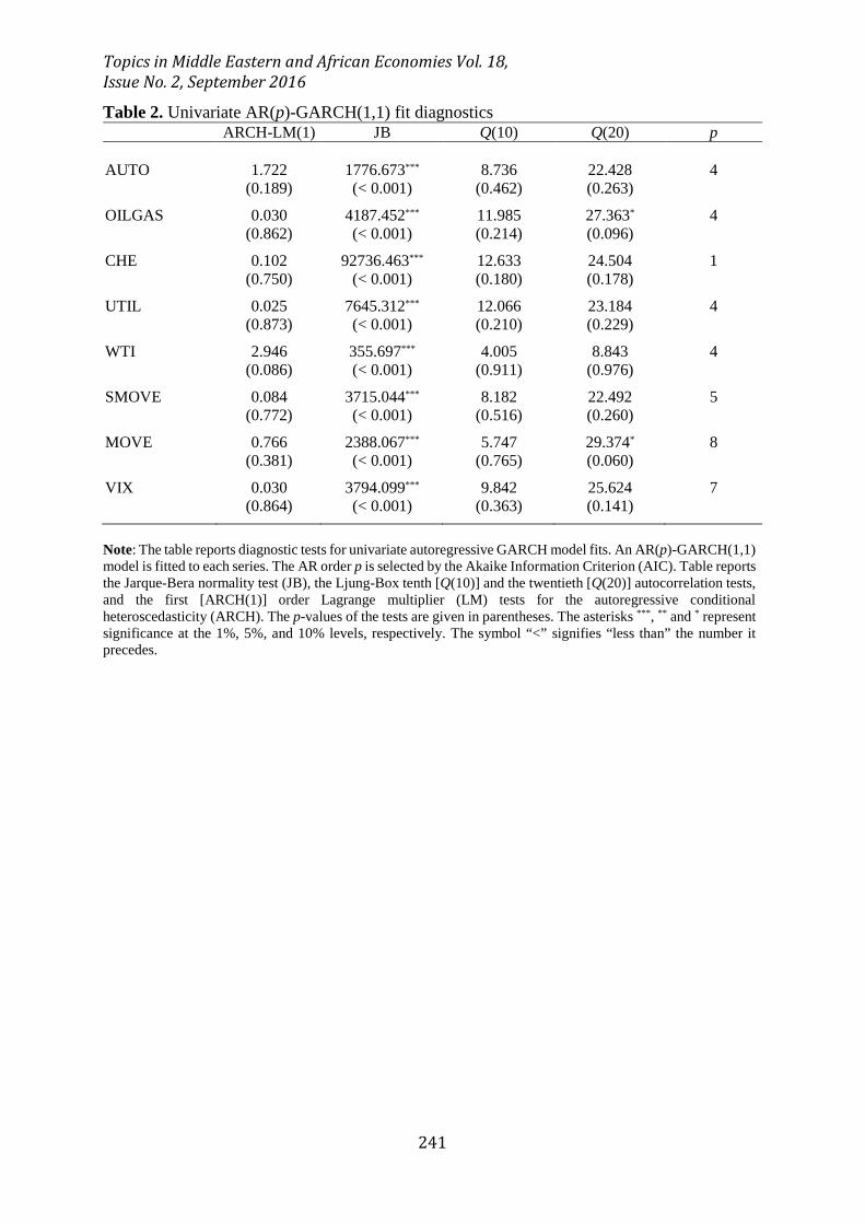
3.3. Dynamic Interdependencies in Returns: VAR Model

We employed a VAR model to have an idea about the return behavior for each of the four

sectors’ CDS indices: WTI, MOVE, SMOVE and VIX. The residuals of the VAR model were used

for the following pursuits about volatility. In our model, we estimated the lags via information selection

criteria. As shown in Table 2, lags are representing for each as p. Diagnostic tests are also shown in

Table 2 for univariate GARCH(1,1) model. All residuals of time series were tested by ARCH-LM(1)

and checked for Jarque-Bera. According to results, ARCH-LM(1) test rejected the null hypothesis

because none of the tests was significant. As a result, we can conclude that there is ARCH effect in all

series. Jarque-Bera tests were checked for normality assumption and was found that is violated at 1%

significance level. The Box–Pierce Portmanteau Q statistics for lagged 10 and lagged 20 orders were

also calculated. Only OILGAS and MOVE are independently distributed for lagged 20. In sum,

according to statistical results, tests and VAR model demonstration that are more suitable to implement


227

Student’s t distribution to the series’ error terms instead of normal distribution.

3.4. Dynamic Interdependencies in Volatilities: BEKK Model

For modelling vectors of residuals, BEKK Engle and Kroner, 1995 GARCH model was used

in analyses. In the VAR model, for return behavior of variables we identified error terms, 𝜀𝜀𝑡𝑡 as:

𝜀𝜀𝑡𝑡 = 𝐻𝐻𝑡𝑡1/2𝑧𝑧𝑡𝑡 Eq. 2

where 𝑧𝑧𝑡𝑡is the 8*1 random vector: 𝑧𝑧𝑡𝑡∼ (0, 𝐼𝐼𝑁𝑁). 𝐼𝐼𝑁𝑁 is the identity matrix of order 8. 𝐻𝐻𝑡𝑡is 8*8 positive

definite symmetric matrix and identified in the BEKK(1, 1) model as:

𝐻𝐻𝑡𝑡 = 𝐶𝐶 𝐶𝐶′ + 𝐴𝐴𝜀𝜀𝑡𝑡−1𝜀𝜀𝑡𝑡−1′ 𝐴𝐴′ + 𝐵𝐵𝐻𝐻𝑡𝑡−1𝐵𝐵′ Eq. 3

where C is upper triangular matrix; A, B are all 8*8 parameter matrices in the model.

Matrix A in Eq. 3 measures the correlation between conditional variances and past squared one-

lag unexpected returns. In other words, Matrix A shows the effects of the selected shocks on volatilities.

On the other hand, Matrix B measures whether the current levels of the conditional variance-covariance

matrix are correlated to past one-lag conditional variance-covariance matrices.

As we discussed earlier, all return series are distributed non-normal as can be seen in Table 1

and 2. Therefore, we checked the distribution of error terms, 𝜀𝜀𝑡𝑡, by using Student’s t distribution.

Figure 1 provides the daily levels of the CDS Premiums, oil price and volatility indices for the

period 1/6/2004-2/2/2016. CDS Premium levels of AUTO and CHE have the peak values in 2009

particularly AUTO reaching the highest CDS level. They also show very similar profile over time,

suggesting they are affected from the similar events and their responses are similar. On the other hand,

OILGAS and UTIL are highly affected from different shocks compared to AUTO and CHE. WTI has

the peak value in mid-2008. The rate of change in WTI is very high between 2007 and 2009. After the


228

peak value for the selected time, WTI decreases rapidly from about $145/gallon to $40/gallon in

approximately six months. After the effects observed in mid-2008, WTI increases with a rate of change

similar to the pre-shocks period until mid-2014. The volatility indices SMOVE and MOVE have very

similar profiles during the chosen time period. The effects of the shocks and the responses of MOVE

and SMOVE are very similar to each other. The interdependency of MOVE and SMOVE are also

observed considering the Pearson Correlation Coefficient (PCC), as observed in Table 1. VIX is also

affected from the similar shocks i.e. reaching the peak value in 2009, as for the other risk measures.

Considering the CDS premiums, WTI and volatility indices; the effects of the different shocks can be

clearly seen. However, the effects of the dominant shocks such as observed around 2009 are temporary

for the selected time period except for the CDS of OILGAS so that the values of the risk measures

become very similar to pre-shock period, after the shocks.

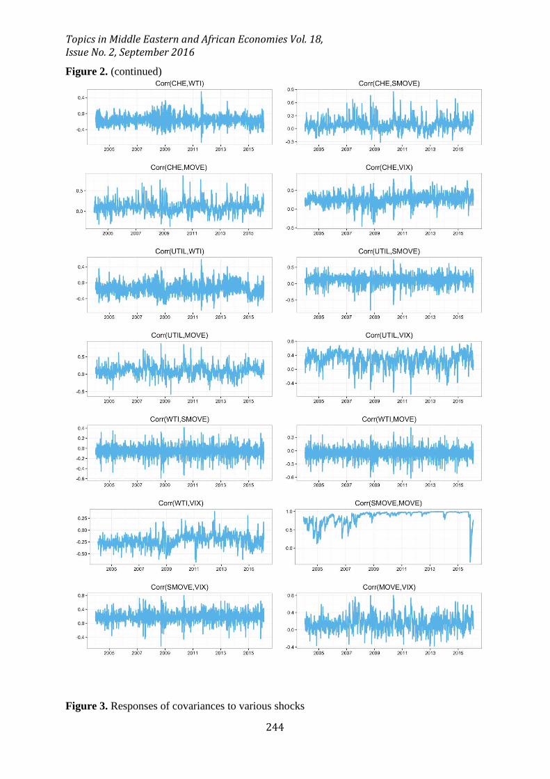
Figure 2 shows the estimated conditional correlations obtained from the BEKK-GARCH

model with a Student's t-distribution. All eight variables that we use in our study show signs of

volatility clustering. They all have upwards and downwards during the time depending on the different

shocks. As can be observed from Figure 2, conditional correlation between MOVE and SMOVE is

generally close to 1 during the chosen time period and volatility is very low compared to other

conditional correlations, which can be expected owing to high interdependency between these two risk

measures as observed in Table 1 and Figure 1.

Highest volatility can be seen between AUTO-CHE in 2007 and 2009 and CHE-UTIL in 2013.

Therefore, it can be concluded that high volatilities of AUTO-CHE and CHE-UTIL are due to different

shocks, i.e. they have low interdependency. On the other hand, lowest volatilities are observed between

WTI-SMOVE/MOVE and WTI-VIX, considering the peak-to-valley differences of the conditional

correlations.


229

General conditional correlation trend between four CDS Premiums are positive and their

profiles suggest volatility between these measures. Conditional correlations between AUTO and the

other CDS Premiums (CHE, OILGAS and UTIL) have high downward peak around 2009, which can

be correlated with Lehman Brothers Bankruptcy shock. However, same trend between each four CDS

Premiums and WTI are negative but close to zero whereas the trend between each four CDS Premiums

and VIX is positive, except the steep upwards and downwards due to different responses of the risk

measures against different shocks. Conditional correlations between each four CDS Premiums and

MOVE/SMOVE are generally close to zero except the responses against the shocks encountered

during the time period. Slight positive conditional correlation can be observed between

MOVE/SMOVE and VIX having similar volatility levels.

4. METHODOLOGY of VIRF and EMPIRICAL RESULTS

4.1. Independent Shocks

In this section, we defined our model used to examine the risk spillover mechanism across the

oil market, financial market, and the oil related Credit Default Swap (CDS) sectors. In addition to

showing the magnitude of the volatility transmission, we described the methodology of the volatility

impulse responses. This method has the advantage of providing valuable information on the speed of

risk transmission. The shape and sign of the volatility impulse responses also provide significant

information.

News or shocks are inherently independent over time as introduced as a new concept by Hafner

and Herwartz, 2006. A shock is a risk source that is independent and unpredictable. It is also shown

that two shocks appearing in different series at the same time are independent. The residuals include

the effects of the shocks coming from independent sources. However, in order to obtain the pure impact

of the shock, the orthogonality conditions of the error terms should be investigated. Otherwise, total

effect of one shock on all the components of the residual would be observed. In order to avoid


230

orthogonality problem, Hafner and Herwartz, 2006 applied Jordan decomposition to retrieve an

independent and realistic shock from the conditionally heteroskedastic error terms.

The component of our model that shows the effect of a shock is named as 𝑧𝑧𝑡𝑡 in 𝜀𝜀𝑡𝑡 by Choleski

decomposition. Independent news could be identified via Jordan decomposition of 𝐻𝐻𝑡𝑡 . Let Λit =

diag (λ1t, … , λNt)is the diagonal matrix whose components λit, 𝑖𝑖 = 1, … ,𝑁𝑁denote the eigenvalues of

𝐻𝐻𝑡𝑡.Γ𝑖𝑖𝑡𝑡 = (𝛾𝛾1𝑡𝑡, … , 𝛾𝛾𝑁𝑁𝑡𝑡) is the matrix N*N whose components Γ𝑖𝑖𝑡𝑡, 𝑖𝑖 = 1, … ,𝑁𝑁 denote the corresponding

eigenvectors. The symmetric matrix of 𝐻𝐻𝑡𝑡1/2can be decomposed as;

𝐻𝐻𝑡𝑡1/2 = 𝛤𝛤𝑡𝑡Λt1/2𝛤𝛤𝑡𝑡′ Eq. 4

As Hafner and Herwartz, 2006 identified 𝑧𝑧𝑡𝑡 as shocks from the past that were able to affect the markets

in the future. Therefore, the independent shocks are defined as;

𝑧𝑧𝑡𝑡 = 𝐻𝐻𝑡𝑡−1/2𝜀𝜀𝑡𝑡 Eq. 5

4.2. Volatility Impulse Response Function (VIRF)

According to Bollerslev et al., 1988 the BEKK (1,1) model for multivariate GARCH models

can be written by using Vector Error Correction (VEC) model representation as follows:

𝑣𝑣𝑣𝑣𝑣𝑣ℎ(𝐻𝐻𝑡𝑡) = 𝑣𝑣𝑣𝑣𝑣𝑣ℎ(𝐶𝐶) + 𝐴𝐴 𝑣𝑣𝑣𝑣𝑣𝑣ℎ(𝜀𝜀𝑡𝑡−1𝜀𝜀𝑡𝑡−1′ ) + 𝐵𝐵 𝑣𝑣𝑣𝑣𝑣𝑣ℎ(𝐻𝐻𝑡𝑡−1) Eq. 6

in which 𝐻𝐻𝑡𝑡 is the conditional covariance matrix at time t and 𝑣𝑣𝑣𝑣𝑣𝑣ℎ(𝐻𝐻𝑡𝑡) indicates the operator that

stacks the lower fraction of an 8*8 matrix into an N*=(N(N+1)/2) dimensional vector. 𝑣𝑣𝑣𝑣𝑣𝑣ℎ(𝐶𝐶) is a

vector which contains N* coefficients, A and B are the parameter matrices containing (N*)2

parameters. This VEC model is used to eliminate the variables of the conditional covariance matrix

that appear twice in the model.


231

According to Hafner and Herwartz, 2006, VIRF is the expectation of volatility conditional on

an initial shock and history subtracted by the baseline expectation that only conditional on history,

which can be written as follows;

𝑉𝑉ℎ(𝑧𝑧𝑡𝑡) = 𝐸𝐸��𝑣𝑣𝑣𝑣𝑣𝑣ℎ(𝐻𝐻𝑡𝑡)�𝜓𝜓𝑡𝑡−1,𝑧𝑧𝑡𝑡�� − 𝐸𝐸[(𝑣𝑣𝑣𝑣𝑣𝑣ℎ(𝐻𝐻𝑡𝑡)|𝜓𝜓𝑡𝑡−1 )] Eq. 7

where 𝑧𝑧𝑡𝑡 is the specific shock affecting the system at time t and 𝜓𝜓𝑡𝑡−1 is the observed history up to time

t – 1. 𝑉𝑉ℎ(𝑧𝑧𝑡𝑡) is the N* = (N (N + 1)/2) vector of the impact of the identical and independent shock

components of 𝑧𝑧𝑡𝑡on the h-step ahead expected conditional variance-covariance matrix components.

Therefore, to find the Eq. 7, the expectation matrix influenced by only history is subtracted from the

h-step ahead expected conditional covariance matrix of a given shock and history. As a result, the

model of 𝑉𝑉ℎ(𝑧𝑧𝑡𝑡) shows the reaction of the conditional variance of the eight variables respectively to

the shock, 𝑧𝑧𝑡𝑡 that occurred h period ago. One-step ahead VIRF applied to a BEKK(1,1) model is,

𝑉𝑉1(𝑧𝑧𝑡𝑡) = 𝐴𝐴 �𝑣𝑣𝑣𝑣𝑣𝑣ℎ �𝐻𝐻𝑡𝑡1/2𝑧𝑧𝑡𝑡𝑧𝑧𝑡𝑡′𝐻𝐻𝑡𝑡

1/2� − 𝑣𝑣𝑣𝑣𝑣𝑣ℎ(𝐻𝐻𝑡𝑡)� = 𝐴𝐴 𝐷𝐷𝑁𝑁+�𝐻𝐻𝑡𝑡1/2 ⊗ 𝐻𝐻𝑡𝑡

1/2�𝐷𝐷𝑁𝑁 𝑣𝑣𝑣𝑣𝑣𝑣ℎ(𝑧𝑧𝑡𝑡𝑧𝑧𝑡𝑡′ − 𝐼𝐼𝑁𝑁)

Eq. 8

where 𝐷𝐷𝑁𝑁 is the duplication matrix defined from the property as:

𝑣𝑣𝑣𝑣𝑣𝑣ℎ (𝑍𝑍) = 𝐷𝐷𝑁𝑁 𝑣𝑣𝑣𝑣𝑣𝑣ℎ(𝑍𝑍) Eq. 9

for any symmetric N*N matrix 𝑍𝑍and 𝐷𝐷𝑁𝑁+ is its Moore-Penrose inverse. 𝐼𝐼𝑁𝑁 is the identity matrix

and 𝐻𝐻𝑡𝑡 is the conditional variance-covariance matrix representation at time t.⊗ represents the

Kronecker product. For h>1, the new VIRF is;

𝑉𝑉ℎ(𝑧𝑧𝑡𝑡) = (𝐴𝐴 + 𝐵𝐵)ℎ−1 𝐴𝐴 𝐷𝐷𝑁𝑁+�𝐻𝐻𝑡𝑡1/2 ⊗ 𝐻𝐻𝑡𝑡

1/2�𝐷𝐷𝑁𝑁𝑣𝑣𝑣𝑣𝑣𝑣ℎ(𝑧𝑧𝑡𝑡𝑧𝑧𝑡𝑡′ − 𝐼𝐼𝑁𝑁) = (𝐴𝐴 + 𝐵𝐵)𝑉𝑉ℎ−1(𝑧𝑧𝑡𝑡) Eq. 10

Compared to the traditional Choleski decomposition impulse response function of the conditional

mean in linear models, VIRF model defined by Hafner and Herwartz, 2006 has the following important


232

properties:

1) The VIRF is an even, symmetric function of the shock with the property of 𝑉𝑉ℎ(𝑧𝑧𝑡𝑡) =

𝑉𝑉ℎ(−𝑧𝑧𝑡𝑡). The impulse responses are odd functions in traditional linear analysis.

2) The VIRF is not homogenous function of any degree while the traditional linear analyses are.

3) The VIRF depends on the history through the volatility state 𝐻𝐻𝑡𝑡 at the time of the initial shock

occurs. However, the traditional analysis on linear systems does not depend on the historic

shocks.

4) The persistence of shocks is calculated in moving average part same in the traditional,

(𝐴𝐴 + 𝐵𝐵)ℎ−1 𝐴𝐴.

In our application, 𝑧𝑧𝑡𝑡 was chosen as a shock with an independent and identically distributed random

variable. The impact of a historical random shock was calculated by the observed volatility when a

shock occurs. However, we are interested in the past events that have an impact on today and future.

In the next part, the impact of observed historical shocks with observed volatilities will give

information about past events.

4.3. Impacts of Historical Shocks on Volatilities

In the sample period, several shocks and effects were witnessed owing to our VIRF analysis.

We focused on specific historical shocks: the US Mortgage Crisis: Lehman Brothers Bankruptcy,

Greece Debt Crises, Fear Of Greece's Default, Egyptian Political Unrest (Second Revolution),

European Sovereign Debt Crisis and US Government Shutdown that have significant effects on our

variables. According to our best knowledge, the impacts of the listed six shocks within and across the

oil related markets and financial market risks have not been considered in VIRF analyses in the

literature. These events are explained below.


233

Lehman Brothers, one of the financial services firms in US, declared bankruptcy on September

15, 2008. This was the largest bankruptcy announcement in US history. The main reason for the

bankruptcy can be associated with large decline of home prices after the collapse in mortgage market.

The starting point of US Mortgage Crisis was accepted as the announcement of the bankruptcy of

Lehman Brothers. This event influenced all the markets significantly not in the US but also worldwide.

In our analysis, September 17, 2008 was accepted as the base point and we investigated the effects of

this event, named also as shock, on our risk transmission and correlation analysis after this date.

Greece was accepted to the European Union on January 1, 1981. Gross Domestic Product

(GDP) per capita reached the highest values in 2008, as around $31,700 after adapting to the currency

of Euro in 2001. The second shock we selected is “Greece Debt Crisis” started officially on December

8, 2009 when country’s credit rating was downgraded by Fitch from A− to BBB+. On March 4, 2010,

Government announced austerity plan. In April 23, 2010 third shock in our analysis, “Fear of Greece’s

Default” was assumed to be started after George Papandreou, Prime Minister of that time, called for a

EU/IMF rescue package of €500bn for 3 years. This rescue package was not enough and second Greek

crisis began because of Greek budget deficit was declared as higher than expected in April 2011. After

that, credit rating of Greece was decreased from B to CCC. Second bailout loan was confirmed for

€130bn. Therefore, interest rate increased and bond prices decreased. Banks and Greek Stock

Exchanged Market closed for a month in June 2015. Unemployment rate was rising to 24.5% in

November 2015. As a result, confidence in Government services was at a low point and the crisis is

still continuing.

In Egypt, thousands of people protested for the step down of Husni Mubarak, the President for

30 years, and for changing the regime to democracy. Police used violence to stop protestors on the

streets, resulting injuries and deaths. First revolution of Egypt named the Arab Spring was on January

25, 2011 where Muslim Brotherhood was a large part of the protests. Demonstrators filled Gharbeya,

Alexandria, Suez, Ismailia and also Tahrir Square in Cairo on May 27, 2011, which was accepted as


234

the base point in our analysis. The demands of the crowd were for civilians not to be judged in military

trials, all members of the Mubarak regime and those who killed protestors to be put on trial. And before

parliament elections, demonstrators wanted the restoration of the Egyptian Constitution.

European Sovereign Debt Crisis started at the end of 2009 around European Union because of

having difficulties in refinancing government debts or repayments of loans to Eurozone countries,

European Central Bank (ECB) and International Monetary Fund (IMF). Increase in Government

expenditures and investments, troubles in housing market therefore in banking system, small economic

growth and also low productivity were main reasons for crisis especially around these Eurozone

member countries; i.e. Greece, Portugal, Ireland, Spain and Cyprus. The effect of Sovereign Debt

Crisis was not only on the entire Eurozone but also on European Union countries and worldwide.

The two chambers of US Congress could not be agree on the offer of increasing the Federal

Government’s debt ceiling or called extra fund to finance Patient Protection and Affordable Care Act

known as Obamacare signed in 2010. As a result, US Government was shutdown on 1st of October

until October 16, 2013. Non-compulsory expenditures were stopped and government postponed

payments. Approximately 800,000 federal employees were forced for an unpaid leave. This event

influenced financial agents and markets negatively, as can be expected. The base shock date chosen

for our analyses was a day ago from the beginning of shutdown.

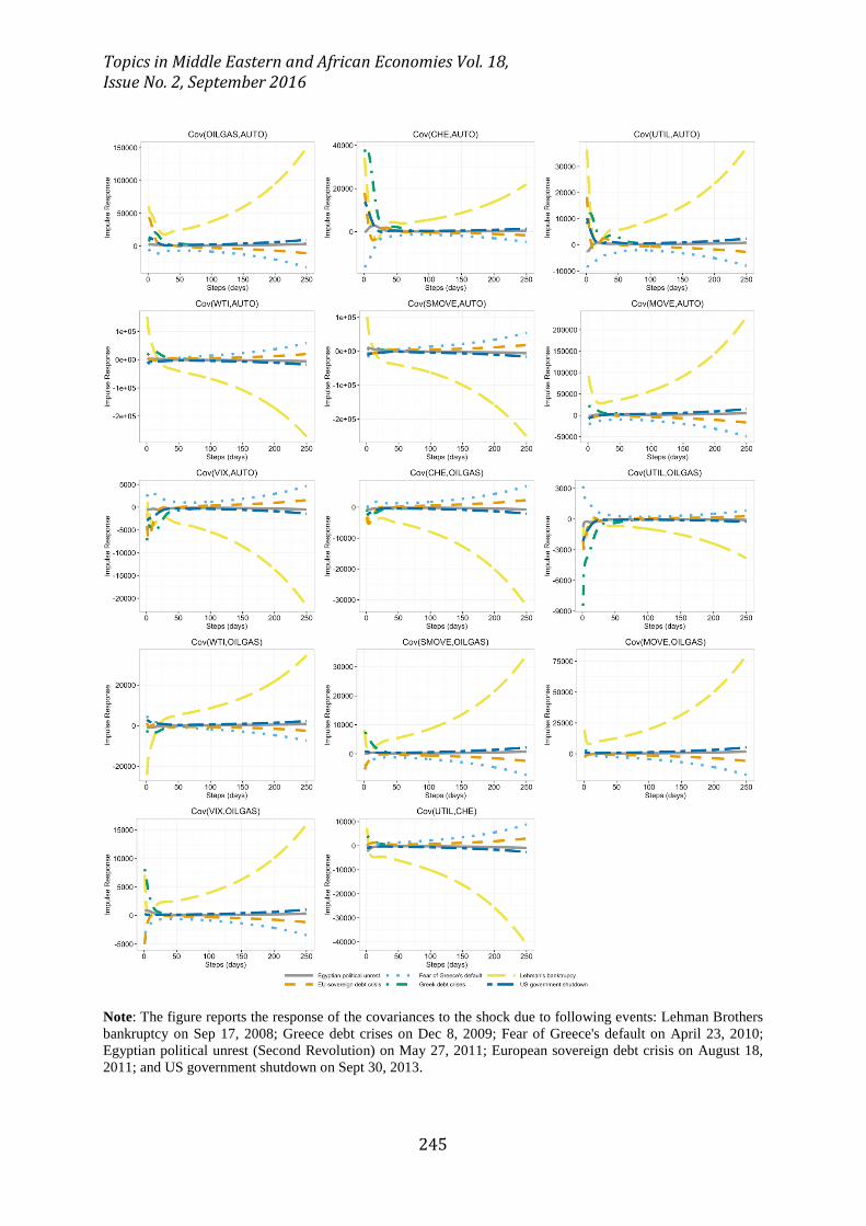
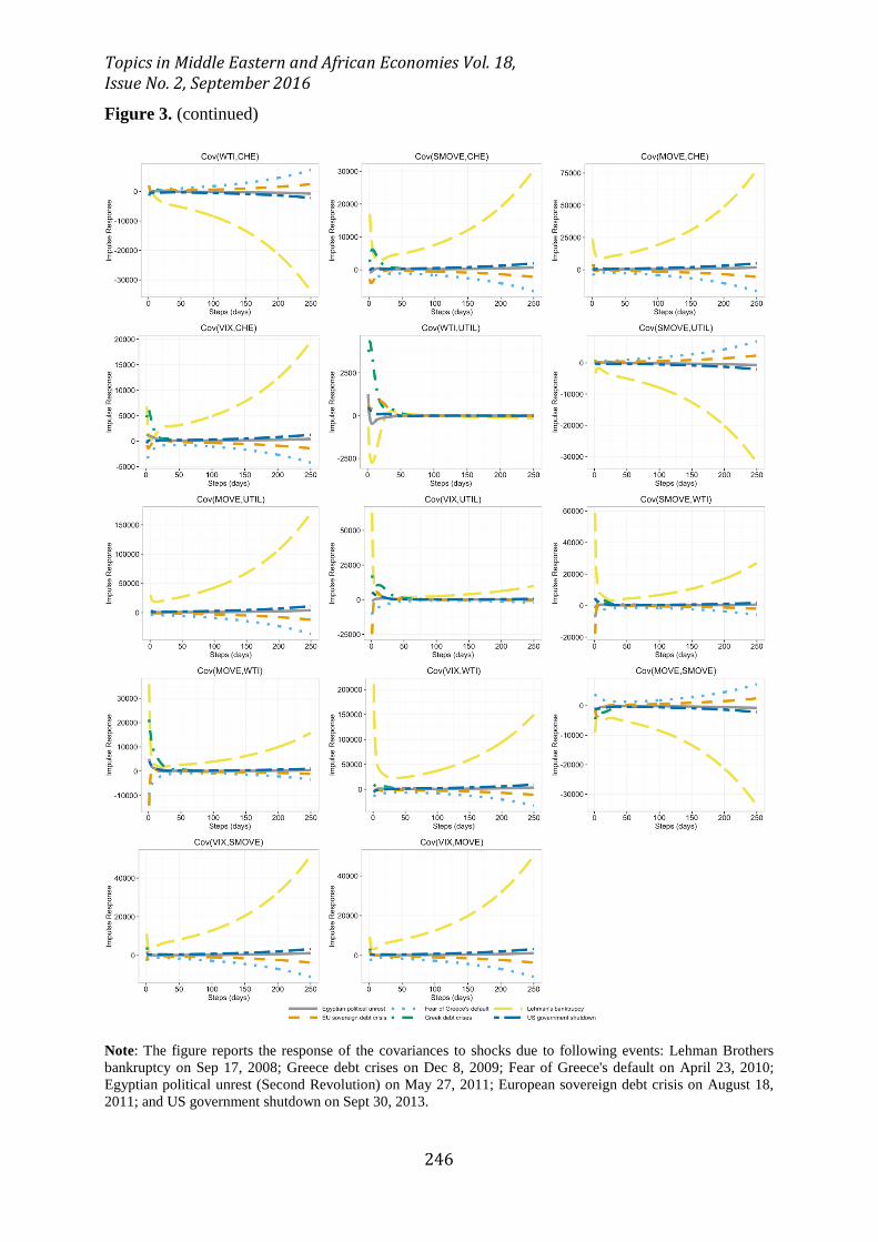
Figure 3 reports the responses to the above listed shocks as Impulse Response to covariances

of eight variables used in this study. Nonzero positive impulse responses imply risk transmission. We

note that some of the shocks might be negative at the date shock and the impulse response might

negative. However, negative impulse responses still imply risk transmission. This is due the fact that

the shocks are not normalized in terms of sign and the size. As can be seen, significant but various

types of responses can be observed for all the covariances due to Lehman Brothers Bankruptcy. This

https://en.wikipedia.org/wiki/Eurozone


235

event or shock has the highest influence on the reported covariances compared to other five events.

Since all the variables used in this study are US-based, higher influence of Lehman Brothers

Bankruptcy to response of covariances can be expected.

Our findings show that covariances of VIX-AUTO, CHE-OILGAS, UTIL-OILGAS, WTI-

CHE, SMOVE-UTIL and MOVE-SMOVE have negative responses to Lehman Brothers Bankruptcy

shock and negative responses tend to be higher in the long run. Covariances of WTI-AUTO, SMOVE-

AUTO and UTIL-CHE shift their response from positive to negative whereas the change of covariance

of WTI-OILGAS is vice-versa. The change in response occurs after a very short time from Lehman

Brothers Bankruptcy. The rest of the covariances show positive response to this shock, however, their

profiles are different. In addition, right after the shock, the covariances have slight positive response,

which tend to become zero in the short run and have increase in the long run except CHE-AUTO,

UTIL-AUTO, VIX-UTIL, SMOVE-WTI, MOVE-WTI and VIX-WTI.

After Lehman Brothers Bankruptcy, the second highest influential shock is the Greece Debt

Crisis. Substantial positive responses of covariances of OILGAS-AUTO, CHE-AUTO, WTI-AUTO,

MOVE-AUTO, VIX-UTIL and MOVE-WTI as well as slight negative response of covariance UTIL-

OILGAS can be observed right after the shock. However, all the responses diminish in the long run.

The other shocks namely Fear of Greece’s Default, European Sovereign Debt Crisis and US

Government Shutdown have very similar effect on the covariances. They have slight effect on

covariances in the short-run, which tends to become zero in the medium term. However, the responses

of the covariances of the risk measures slightly increase as time passes. Another remarkable feature is

that covariances tend to show higher response to Fear of Greece’s Default compared to European

Sovereign Debt Crisis and US Government Shutdown in the long term. In this respect, the lowest

response is to US Government Shutdown.

Covariances of the all the risk measures are almost insensitive to Egyptian Political Unrest.


236

Furthermore, the covariance of WTI-UTIL has no significant response to all reported shocks since

utilities are a local monopoly that are regulated by policymakers. Moreover, utilities do not use oil as

a fuel.

5. Conclusion

The study examines the volatility transmission mechanism across the oil and financial markets and

sector CDSs, using eight different measures of risks during the period January 6, 2004 –February 2,

2016. In addition to assessing the magnitude of the volatility transmission, the volatility impulse

responses have the advantage of providing valuable information on the speed of risk transmission. The

shape and sign of the volatility impulse responses also provide significant information on the

transmission mechanism. We also evaluate the risk transmission due to global shocks related to the

US Mortgage Crisis, Lehman Brothers Bankruptcy, Greece Debt Crisis, Fear of Greece's Default,

Egyptian Political Unrest (Second Revolution), European Sovereign Debt Crisis and US Government

Shutdown and observe that most of these events lead to significant risk transmission. Among these

events, the Lehman Brothers Bankruptcy has destabilizing effects on all the oil-related sectors. We

also find that all oil market related shocks have significant risk transmission effects. Finally, the results

show complicated transmission mechanisms that spread over long periods.


237

References

Adams Z, Füss R, Schindler F. The Sources of Risk Spillovers among U.S. REITs: Financial

Characteristics and Regional Proximity. Real Estate Economics 2015;43; 67-100.

Beaudry P, Koop G. Do recessions permanently change output? Journal of Monetary Economics

1993;31; 149-163.

Becker KG, Finnerty JE, Gupta M. The Intertemporal Relation Between the U. S. and Japanese

Stock Markets. The Journal of Finance 1990;45; 1297-1306.

Becker R, Clements AE, McClelland A. The jump component of S&P 500 volatility and the

VIX index. Journal of Banking & Finance 2009;33; 1033-1038.

Berndt A, Douglas R, Duffie D, Ferguson M, Schranz D. Measuring Default Risk Premia from

Default Swap Rates and EDFs. BIS Working Paper No. 173; EFA 2004 Maastricht Meetings

Paper No. 5121. . Available at SSRN: http://ssrn.com/abstract=556080 2008.

Bharath ST, Shumway T. Forecasting Default with the KMV-Merton Model. Available at SSRN:

http://ssrn.com/abstract=637342 2004.

Blanchard OJ, Quah D. The Dynamic Effects of Aggregate Demand and Supply Disturbances. The

American Economic Review 1989;79; 655-673.

Bollerslev T, Engle R, Wooldridge J. A Capital Asset Pricing Model with Time-Varying

Covariances. Journal of Political Economy 1988;96; 116-131.

Booth GG, Chowdhury M, Martikainen T, Tse Y. Intraday Volatility in International Stock Index

Futures Markets: Meteor Showers or Heat Waves? Management Science 1997;43; 1564-

1576.

Byström H. Credit Default Swaps and Equity Prices: The iTraxx CDS Index Market. Financial

Analysts Journal 2006;62; 65-76.

Das SR, Hanouna P. Credit default swap spreads. Journal of Investment Management 2006;4; 93-

105.

Diebold FX, Yilmaz K. Measuring Financial Asset Return and Volatility Spillovers, with

Application to Global Equity Markets*. The Economic Journal 2009;119; 158-171.

Doan T, Litterman RB, Sims CA. Forecasting and Conditional Projection Using Realistic Prior

Distributions. National Bureau of Economic Research Working Paper Series 1983;No. 1202.

Engle RF, Ito T, Lin W-L. Meteor Showers or Heat Waves? Heteroskedastic Intra-Daily Volatility in

the Foreign Exchange Market. Econometrica 1990;58; 525-542.

Engle RF, Kroner KF. Multivariate Simultaneous Generalized Arch. Econometric Theory 1995;11;

122-150.

http://ssrn.com/abstract=556080



238

Engle RF, Ng VK. Measuring and Testing the Impact of News on Volatility. The Journal of Finance

1993;48; 1749-1778.

Ericsson J, Jacobs K, Oviedo R. The Determinants of Credit Default Swap Premia. Journal of

Financial and Quantitative Analysis 2009;44; 109-132.

Eun CS, Shim S. International Transmission of Stock Market Movements. The Journal of Financial

and Quantitative Analysis 1989;24; 241-256.

Ewing BT, Malik F, Ozfidan O. Volatility transmission in the oil and natural gas markets. Energy

Economics 2002;24; 525-538.

Fernandes M, Medeiros MC, Scharth M. Modeling and predicting the CBOE market volatility index.

Journal of Banking & Finance 2014;40; 1-10.

Figuerola-Ferretti I, Paraskevopoulos I, 2011. Pairing market risk with credit risk. Universidad

Carlos III, Departamento de Economía de la Empresa.

Forte S, Lovreta L. Credit Risk Discovery in the Stock and CDS Markets: Who Leads, When, and

Why. Available at SSRN: http://ssrn.com/abstract=1183202 2008.

Forte S, Peña JI. Credit spreads: An empirical analysis on the informational content of stocks, bonds,

and CDS. Journal of Banking & Finance 2009;33; 2013-2025.

Fung H-G, Sierra GE, Yau J, Zhang G. Are the U.S. Stock Market and Credit Default Swap Market

Related? Evidence from the CDX Indices. Journal of Alternative Investments 2008;11; 43-61.

Gallant A, Rossi P, Tauchen G. Nonlinear Dynamic Structures. Econometrica 1993;61; 871-907.

Grobys K. Have volatility spillover effects of cointegrated European stock markets increased over

time? . The Review of Finance and Banking 2010;02; 83-94.

Hafner CM, Herwartz H. Volatility impulse responses for multivariate GARCH models: An

exchange rate illustration. Journal of International Money and Finance 2006;25; 719-740.

Hamao Y, Masulis RW, Ng V. Correlations in Price Changes and Volatility across International

Stock markets. Review of Financial Studies 1990;3; 281-307.

Hammoudeh S, Liu T, Chang C-L, McAleer M. Risk spillovers in oil-related CDS, stock and credit

markets. Energy Economics 2013;36; 526-535.

Jarque CM, Bera AK. Efficient tests for normality, homoscedasticity and serial independence of

regression residuals. Economics Letters 1980;6; 255-259.

Karolyi GA. A Multivariate GARCH Model of International Transmissions of Stock Returns and

Volatility: The Case of the United States and Canada. Journal of Business & Economic

Statistics 1995;13; 11-25.

Koch PD, Koch TW. Evolution in dynamic linkages across daily national stock indexes. Journal of

International Money and Finance 1991;10; 231-251.



239

Koop G, Pesaran MH, Potter SM. Impulse response analysis in nonlinear multivariate models.

Journal of Econometrics 1996;74; 119-147.

Koutmos G, Booth GG. Asymmetric volatility transmission in international stock markets. Journal of

International Money and Finance 1995;14; 747-762.

Le Pen Y, Sévi B. Volatility transmission and volatility impulse response functions in European

electricity forward markets. Energy Economics 2010;32; 758-770.

Lee KC, Pesaran MH. Persistence profiles and business cycle fluctuations in a disaggregated model

of U.K. output growth. Ricerche Economiche 1993;47; 293-322.

Lin W-L. Impulse Response Function for Conditional Volatility in GARCH Models. Journal of

Business & Economic Statistics 1997;15; 15-25.

Lin W-L, Engle RF, Ito T. Do Bulls and Bears Move Across Borders? International Transmission of

Stock Returns and Volatility. Review of Financial Studies 1994;7; 507-538.

Longstaff FA, Mithal S, Neis E. Corporate Yield Spreads: Default Risk or Liquidity? New Evidence

from the Credit Default Swap Market. The Journal of Finance 2005;60; 2213-2253.

Luo X, Zhang JE. The Term Structure of VIX. Journal of Futures Markets 2012;32; 1092-1123.

Norden L, Weber M. The Co-movement of Credit Default Swap, Bond and Stock markets: an

Empirical Analysis. European Financial Management 2009;15; 529-562.

Panopoulou E, Pantelidis T. Integration at a cost: evidence from volatility impulse response

functions. Applied Financial Economics 2009;19; 917-933.

Pesaran MH, Pierse RG, Lee KC. Persistence, cointegration, and aggregation. Journal of

Econometrics 1993;56; 57-88.

Pesaran MH, Potter SM. A floor and ceiling model of US output. Journal of Economic Dynamics

and Control 1997;21; 661-695.

Potter SM. A nonlinear approach to US GNP. Journal of Applied Econometrics 1995;10; 109-125.

Serletis A, Shahmoradi A. Measuring and Testing Natural Gas and Electricity Markets Volatility:

Evidence from Alberta's Deregulated Markets. Studies in Nonlinear Dynamics &

Econometrics 2006;10; 1-20.

Sims CA. Macroeconomics and Reality. Econometrica 1980;48; 1-48.

Zhang BY, Zhou H, Zhu H. Explaining Credit Default Swap Spreads with the Equity Volatility and

Jump Risks of Individual Firms. Review of Financial Studies 2009;22; 5099-5131.

Zhu H. An Empirical Comparison of Credit Spreads between the Bond Market and the Credit

Default Swap Market. Journal of Financial Services Research 2006;29; 211-235.


240

Table 1. Descriptive Statistics and Correlations Mean S.D. Min Max Skewness Kurtosis JB Q(1) Q(4) ARCH(1) ARCH(4) Panel A: Descriptive statistics for log returns (%) AUTO 0.01% 4.67% -141.40% 46.41% -8.74% 281.68% 10470537.58*** 102.62*** 131.94*** 8.11*** 24.64*** OILGAS 0.07% 3.53% -96.78% 40.23% -6.40% 210.65% 5854834.47*** 29.89*** 49.31*** 7.84*** 10.78* CHE 0.01% 4.44% -126.93% 86.65% -5.18% 283.69% 10593977.62*** 13.03*** 42.56*** 18.15*** 25.44*** UTIL 0.02% 5.46% -241.70% 20.65% -29.36% 1244.67% 204108753.82*** 12.45*** 246.59*** 0.00 70.16*** WTI 0.00% 2.09% -10.58% 12.12% -0.13% 3.09% 1264.83*** 11.44*** 21.05*** 96.75*** 415.34*** SMOVE -0.02% 5.16% -139.32% 137.89% 0.02% 329.09% 14237272.92*** 125.83*** 139.69*** 776.51*** 1279.86*** MOVE -0.01% 4.02% -22.21% 30.59% 0.55% 4.97% 3400.14*** 6.24** 45.95*** 24.76*** 73.24*** VIX 0.01% 6.88% -35.06% 49.60% 0.70% 4.03% 2395.49*** 27.79*** 47.04*** 134.78*** 218.72***

Panel B: Pearson correlation coefficient estimates for the full sample AUTO OILGAS CHE UTIL WTI SMOVE MOVE VIX AUTO 1.000 OILGAS 0.266 1.000 CHE 0.179 0.201 1.000 UTIL 0.141 0.151 0.115 1.000 WTI -0.146 -0.176 -0.065 -0.069 1.000 SMOVE 0.053 0.072 0.056 0.042 -0.046 1.000 MOVE 0.069 0.079 0.076 0.054 -0.056 0.646 1.000 VIX 0.259 0.213 0.143 0.108 -0.234 0.163 0.188 1.000

Panel C: Pearson correlation coefficient estimates for the subprime mortgage crises period (Dec 2007-Jun 2009) AUTO OILGAS CHE UTIL WTI SMOVE MOVE VIX AUTO 1.000 OILGAS 0.339 1.000 CHE 0.069 0.202 1.000 UTIL 0.337 0.831 0.222 1.000 WTI -0.145 -0.226 0.004 -0.240 1.000 SMOVE -0.062 0.140 0.044 0.132 -0.099 1.000 MOVE -0.060 0.139 0.054 0.135 -0.061 0.952 1.000 VIX 0.103 0.235 0.044 0.214 -0.320 0.210 0.183 1.000

Note: Panel A provides the descriptive statistics for log returns. The sample period covers 1/6/2004-2/2/2016 with n=3151 daily observations. AUTO stands for the five-year US auto sector CDS premium; OILGAS stands for the five-year US auto oil and gas sector CDS premium; CHE stands for the five-year US chemicals sector CDS premium; UTIL stands for the five-year US utilities sector CDS premium; WTI stands for the daily closing price for the West Texas Intermediate (WTI) crude oil futures contract 3 (dollars per gallon) delivered in Cushing, Oklahoma; SMOVE stands for one-month bond volatility index; MOVE one-month volatility index for swaption; and VIX stands for the CBOE SPX volatility. In addition to the mean, the standard deviation (S.D.), minimum (min), maximum (max), skewness, and kurtosis statistics, the table reports the Jarque-Bera normality test (JB), the Ljung-Box first [Q(1)] and the fourth [Q(4)] autocorrelation tests, and the first [ARCH(1)] and the fourth [ARCH(4)] order Lagrange multiplier (LM) tests for the autoregressive conditional heteroskedasticity (ARCH). Panels B and C provide the Pearson correlation coefficient (PCC) estimates for the full sample and for the subprime mortgage crises period of Dec. 2007-Jun 2009, respectively. The asterisks ***, ** and * represent significance at the 1%, 5%, and 10% levels, respectively.


241

Table 2. Univariate AR(p)-GARCH(1,1) fit diagnostics ARCH-LM(1) JB Q(10) Q(20) p AUTO 1.722

(0.189) 1776.673*** (< 0.001)

8.736 (0.462)

22.428 (0.263)

4

OILGAS 0.030 (0.862)

4187.452*** (< 0.001)

11.985 (0.214)

27.363* (0.096)

4

CHE 0.102 (0.750)

92736.463*** (< 0.001)

12.633 (0.180)

24.504 (0.178)

1

UTIL 0.025 (0.873)

7645.312*** (< 0.001)

12.066 (0.210)

23.184 (0.229)

4

WTI 2.946 (0.086)

355.697*** (< 0.001)

4.005 (0.911)

8.843 (0.976)

4

SMOVE 0.084 (0.772)

3715.044*** (< 0.001)

8.182 (0.516)

22.492 (0.260)

5

MOVE 0.766 (0.381)

2388.067*** (< 0.001)

5.747 (0.765)

29.374* (0.060)

8

VIX 0.030 (0.864)

3794.099*** (< 0.001)

9.842 (0.363)

25.624 (0.141)

7

Note: The table reports diagnostic tests for univariate autoregressive GARCH model fits. An AR(p)-GARCH(1,1) model is fitted to each series. The AR order p is selected by the Akaike Information Criterion (AIC). Table reports the Jarque-Bera normality test (JB), the Ljung-Box tenth [Q(10)] and the twentieth [Q(20)] autocorrelation tests, and the first [ARCH(1)] order Lagrange multiplier (LM) tests for the autoregressive conditional heteroscedasticity (ARCH). The p-values of the tests are given in parentheses. The asterisks ***, ** and * represent significance at the 1%, 5%, and 10% levels, respectively. The symbol “<” signifies “less than” the number it precedes.


242

Figure 1. Time-series plots of level of the CDS premium, oil price, and volatility indices

Note: This figure provides the plots of the daily levels of the indices for the period 1/6/2004-2/2/2016. AUTO stands for the five-year US auto sector CDS premium; OILGAS stands for the five-year US auto oil and gas sector CDS premium; CHE stands for the five-year US chemicals sector CDS premium; UTIL stands for the five-year US utilities sector CDS premium; WTI stands for the daily closing price for the West Texas Intermediate (WTI) crude oil futures contract 3 (dollars per gallon) delivered in Cushing, Oklahoma; SMOVE stands for one-month bond volatility index; MOVE one-month volatility index for swaption; and VIX stands for the CBOE SPX volatility.


243

Figure 2. Conditional correlations from the BEKK-GARCH model


244

Figure 2. (continued)

Figure 3. Responses of covariances to various shocks


245

Note: The figure reports the response of the covariances to the shock due to following events: Lehman Brothers bankruptcy on Sep 17, 2008; Greece debt crises on Dec 8, 2009; Fear of Greece's default on April 23, 2010; Egyptian political unrest (Second Revolution) on May 27, 2011; European sovereign debt crisis on August 18, 2011; and US government shutdown on Sept 30, 2013.


246

Figure 3. (continued)

Note: The figure reports the response of the covariances to shocks due to following events: Lehman Brothers bankruptcy on Sep 17, 2008; Greece debt crises on Dec 8, 2009; Fear of Greece's default on April 23, 2010; Egyptian political unrest (Second Revolution) on May 27, 2011; European sovereign debt crisis on August 18, 2011; and US government shutdown on Sept 30, 2013.

Documents

On the risk spillover across the oil market, financial …meea.sites.luc.edu/volume18/pdfs/212-On the Risk.pdfmodel, and (2) to discern how major global events affect the volatility