Embed Size (px)
Citation preview

© 2004 SFoCMDOI: 10.1007/s10208-004-0119-0
Found. Comput. Math. 125–144 (2005)
The Journal of the Society for the Foundations of Computational Mathematics
FOUNDATIONS OFCOMPUTATIONALMATHEMATICS
On the Roots of a Random System of Equations. The Theoremof Shub and Smale and Some Extensions
Jean-Marc Azaıs1 and Mario Wschebor2
1Laboratoire de Statistique et ProbabilitesUMR-CNRS C5583 Universite Paul Sabatier118, route de Narbonne31062 Toulouse Cedex 4, [email protected]
2Centro de MatematicaFacultad de CienciasUniversidad de la RepublicaCalle Igua 422511400 Montevideo, [email protected]
Abstract. We give a new proof of a theorem of Shub and Smale [9] on the expec-tation of the number of roots of a system of m random polynomial equations in mreal variables, having a special isotropic Gaussian distribution. Further, we presenta certain number of extensions, including the behavior as m →+∞ of the varianceof the number of roots, when the system of equations is also stationary.
1. Introduction
Let us consider m polynomials in m variables with real coefficients
Xi (t) = Xi (t1, ..., tm), i = 1, ...,m.
Date received: January 8, 2004. Final version received: June 11, 2004. Date accepted: August 4, 2004.Communicated by Steve Smale. Online publication: December 6, 2004.AMS classification: Primary: 60G60, 14Q99. Secondary: 30C15.Key words and phrases: Random polynomials, System of random equations, Rice formula.

126 J.-M. Azaıs and M. Wschebor
We use the notation
Xi (t) :=∑‖ j‖≤di
a(i)j t j , (1)
where j := ( j1, . . . , jm) is a multi-index of nonnegative integers, ‖ j‖ := j1 +· · · + jm , j! := j1! . . . jm!, t j := t j1
1 . . . tjm
m , a(i)j := a(i)j1,..., jm. The degree of the i th
polynomial is di and we assume that di ≥ 1 for all i .Let N X (V ) be the number of roots lying in the subset V of Rm , of the system
of equations
Xi (t) = 0, i = 1, . . . ,m. (2)
We will assume throughout that V is a Borel set with the regularity property thatits boundary has zero Lebesgue measure. We denote N X = N X (Rm).
We will be interested in random real-valued functions Xi (i = 1, . . . ,m),in which case we will call “random fields” the Xi ’s, as well as the Rm-valuedrandom function X (t) = (X1(t), . . . , Xm(t))
T , t ∈ Rm . Whenever the Xi ’s arepolynomials we will say that the Xi ’s and X are “polynomial random fields.”
Generally speaking, little is known on the distribution of N X (V ), even forsimple choices of the law on the coefficients. In the case of one equation in onevariable, a certain number of results have been known for a long time, startingwith the work of Marc Kac [6]. See, for example, the book by Bharucha-Reid andSambandham [2].
Shub and Smale [9] computed the expectation of N X when the coefficients areGaussian, centered independent random variables with certain specified variances(see Theorem 3 below and also the book by Blum et al. [3]). Extensions of theirwork, including new results for one polynomial in one variable, can be found inthe review paper by Edelman and Kostlan [5], see also Kostlan [7].
The primary aim of the present paper is to give a new proof of Shub and Smale’stheorem, based upon the so-called Rice formula to compute the moments of thenumber of roots of random fields. At the same time, this permits certain extensions(some of which are already present in the cited papers by Edelman and Kostlan) toclasses of Gaussian polynomials not considered before, and for which some newbehavior of the number of roots can be observed.
Additionally, in Section 6 we consider nonpolynomial systems such that thelines are independent and the law of each line is centered Gaussian, invariantunder isometries as well as translations. Under general conditions, we are able toestimate a lower bound for the variance of the number of roots and show that, forvery general sets, the ratio of the standard deviation over the mean tends to infinityas the number m of variables tends to infinity.
2. Rice Formulas
In this section we give a brief account without proofs of Rice formulas, containedin the statements of the following two theorems (Azaıs and Wschebor [1]):

Random Systems 127
Theorem 1. Let V be a compact subset of Rm , let Z : V → Rm be a random
field, and let u ∈ Rm be a fixed point.Assume that:
(1) Z is Gaussian.(2) x � Z(x) is almost surely of class C1.(3) For each x ∈ V , Z(x) has a nondegenerate distribution and denote by
pZ(x) its density.(4) P{∃x ∈ V , Z(x) = u, det(Z ′(x)) = 0} = 0. Here, V is the interior of V
and Z ′ denotes the derivative of the field Z(·).(5) λm(∂V ) = 0, where ∂V is the boundary of V and λm is the Lebesgue
measure on Rm (we will also use dx instead of λm(dx)). Then, denotingN Z
u (V ) := �{x ∈ V : Z(x) = u}, one has
E(N Zu (V )) =
∫I
E(| det(Z ′(x))|/Z(x) = u
)pZ(x)(u) dx, (3)
and both members are finite. E(X/·) denotes conditional expectation.
Theorem 2. Let k, k ≥ 2, be an integer. Assume the same hypotheses as inTheorem 1, except for (3) that is replaced by the stronger one:
(3′) for x1, . . . , xk ∈ V pairwise different values of the parameter, the distri-bution of the random vector (Z(x1), . . . , Z(xk)) does not degenerate in(Rm)k and we denote by pZ(x1),...,Z(xk ) its density. Then
E[(N Zu (V ))(N
Zu (V )− 1) . . . (N Z
u (V )− k + 1)]
=∫
V k
E
(k∏
j=1
| det(Z ′(xj ))|/Z(x1) = · · · = Z(xk) = u
)
pZ(x1),...,Z(xk )(u, . . . , u)dx1 . . . dxk, (4)
where both members may be infinite.
If one wants to prove Theorem 1, a direct approach is as follows. Assume that uis not a critical value of Z (this holds true with probability 1 under the hypothesesof Theorem 1). Put n := N Z
u (V ). Since V is compact, n is finite, and if n �= 0,let x (1), . . . , x (n) be the roots of Z(x) = u belonging to V . One can prove thatalmost surely x (i) /∈ ∂V for all i = 1, . . . , n. Hence, applying the inverse functiontheorem, if δ is small enough, one can find in V open neighborhoods U1, . . . ,Un
of x (1), . . . , x (n), respectively, so that:
(1) Z is a C1 diffeomorphism Ui → Bm(u, δ), the open ball centered in u withradius δ, for each i = 1, . . . , n.
(2) U1, . . . ,Un are pairwise disjoint.(3) If x /∈⋃n
i=1 Ui , then Z(x) /∈ Bm(u, δ).

128 J.-M. Azaıs and M. Wschebor
Using the change of variable formula, we have
∫V| det(Z ′(x))|1I{‖Z(x)−u‖<δ} dx =
i=1∑n
∫Ui
| det(Z ′(x))| dx = λm(Bm(u, δ))n.
Hence,
N Zu (V ) = n = lim
δ↓0
1
λm(Bm(u, δ))
∫V| det(Z ′(x))|1I{‖Z(x)−u‖<δ} dx . (5)
If n = 0, (5) is obvious. Now an informal computation of E(N Zu (V )) can be
performed in the following way:
E(N Z
u (V )) = lim
δ↓0
∫Vdx
1
λm(Bm(u, δ))
∫Bm (u,δ)
E(| det(Z ′(x))|/Z(x)= y)pZ(x)(y) dy
=∫
VE(| det(Z ′(x))|/Z(x) = u)pZ(x)(u) dx . (6)
Instead of formally justifying these equalities, the proof in Azaıs and Wschebor[1] goes in fact through a different path. The proof of Theorem 2 is similar.
For Gaussian fields, an essential simplification in the application of Theorem1 comes from the fact that, in this case, orthogonality implies independence andthis is helpful in simplifying the conditional expectation in the integrand.
3. Main Results
We begin with the statement of the Shub and Smale theorem.
Theorem 3 ([9]). Let
Xi (t) =∑‖ j‖≤di
a(i)j t j , i = 1, . . . ,m.
Assume that the real-valued random variables a(i)j are independent Gaussian cen-tered, and
Var(a(i)j
) = ( di
j1 . . . jm
)= di !
j1! . . . jm!(di −∑h=m
h=1 jh)!.
Then,
E(N X ) =√
d, (7)
where d = d1 . . . dm is the Bezout number of the polynomial system X (t).

Random Systems 129
A direct computation shows that under the Shub and Smale hypothesis, theXi ’s are centered independent Gaussian fields, and the covariance function of Xi
is given by
r Xi (s, t) = E(Xi (s)Xi (t)) = (1+ 〈s, t〉)di ,
where 〈s, t〉 denotes the usual scalar product in Rm .More generally, assume that we only require that the polynomial random
fields Xi are independent and that their covariances r Xi (s, t) are invariant un-der isometries of Rm, i.e., r Xi (Us,Ut) = r Xi (s, t) for any isometry U and anypair (s, t). This implies, in particular, that the coefficients a(i)j remain independentfor different i’s but can now be correlated from one j to another for the same valueof i . It is easy to check that this implies that, for each i = 1, . . . ,m, the covariancer Xi (s, t) is a function of the triple
(〈s, t〉, ‖s‖2, ‖t‖2)
(‖·‖ is the Euclidean norm inR
m). It can also be proved (Spivak [10]) that this function is in fact a polynomialwith real coefficients, say Q(i),
r Xi (s, t) = Q(i)(〈s, t〉, ‖s‖2, ‖t‖2), (8)
satisfying the symmetry condition
Q(i)(u, v, w) = Q(i)(u, w, v). (9)
A simple way to construct a class of covariances of this type is to take
Q(i)(u, v, w) = P(u, vw), (10)
where P is a polynomial in two variables with nonnegative coefficients. In fact,consider the two functions defined on Rm × Rm by means of (s, t) � 〈s, t〉and (s, t) � ‖s‖2‖t‖2. It is easy to see that both are covariances of polynomialrandom fields. On the other hand, the set of covariances of polynomial randomfields is closed under linear combinations with nonnegative coefficients as wellas under multiplication, so that P(〈s, t〉, ‖s‖2‖t‖2) is also the covariance of somepolynomial random field.
One can check that using this recipe one cannot construct all the possiblecovariances of polynomial random fields. For example, the following polynomialis a covariance (of some polynomial random field):
r(s, t) = 1+ m + 1
m〈s, t〉2 − 1
m(‖s‖2‖t‖2),
but, if m ≥ 2, it cannot be obtained from the construction of (10).The situation becomes simpler if one considers only functions of the scalar
product, i.e.,
Q(i)(u, v, w) =di∑
k=0
ckuk .
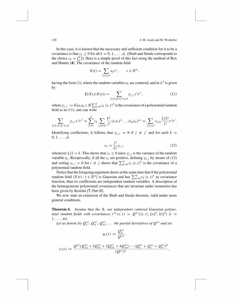
130 J.-M. Azaıs and M. Wschebor
In this case, it is known that the necessary and sufficient condition for it to be acovariance is that ck ≥ 0 for all k = 0, 1, . . . , di . [Shub and Smale corresponds tothe choice ck =
(di
k
)]. Here is a simple proof of this fact using the method of Box
and Hunter [4]. The covariance of the random field
X (t) =∑‖ j‖≤d
aj tj , t ∈ Rm,
having the form (1), where the random variables aj are centered, and in L2 is givenby
E(X (s)X (t)) =∑
‖ j‖≤d,‖ j ′‖≤d
γj, j ′sj t j ′ , (11)
where γj, j ′ := E(aj aj ′). If∑d
k=0 ck 〈s, t〉k is the covariance of a polynomial randomfield as in (11), one can write
∑‖ j‖≤d,‖ j ′‖≤d
γj, j ′sj t j ′ =
d∑k=0
ck
∑‖ j‖=k
k!
j!(s1t1)
j1 . . . (smtm)jm =
∑‖ j‖≤d
c‖ j‖‖ j‖!
j!s j t j .
Identifying coefficients, it follows that γj, j ′ = 0 if j �= j ′ and for each k =0, 1, . . . , d ,
ck = j!
k!γj, j , (12)
whenever ‖ j‖ = k. This shows that ck ≥ 0 since γj, j is the variance of the randomvariable aj . Reciprocally, if all the ck are positive, defining γj, j by means of (12)and setting γi, j = 0 for i �= j shows that
∑dk=0 ck 〈s, t〉k is the covariance of a
polynomial random field.Notice that the foregoing argument shows at the same time that if the polynomial
random field {X (t) : t ∈ Rm} is Gaussian and has∑di
k=0 ck 〈s, t〉k as covariancefunction, then its coefficients are independent random variables. A description ofthe homogeneous polynomial covariances that are invariant under isometries hasbeen given by Kostlan [7, Part II].
We now state an extension of the Shub and Smale theorem, valid under moregeneral conditions.
Theorem 4. Assume that the Xi are independent centered Gaussian polyno-mial random fields with covariances r Xi (s, t) = Q(i)(〈s, t〉, ‖s‖2, ‖t‖2) (i =1, . . . ,m).
Let us denote by Q(i)u , Q(i)
w , Q(i)uv , . . . the partial derivatives of Q(i) and set
qi (x) := Q(i)u
Q(i),
ri (x) := Q(i)(Q(i)uu + 2Q(i)
uv + 2Q(i)uw + 4Q(i)
vw)− (Q(i)u + Q(i)
v + Q(i)w )
2
(Q(i))2,

Random Systems 131
where the functions on the right-hand sides are always computed at the triplet(x, x, x).
Put
hi (x) := 1+ xri (x)
qi (x).
Then, for all Borel sets V with boundary having zero Lebesgue measure, we have
E(N X (V )) = (2π)−m/2Lm−1
∫V
(m∏
i=1
qi (‖t‖2)
)1/2
Eh(‖t‖2) dt. (13)
Here
Eh(x) := E
( m∑
i=1
hi (x)ξ2i
)1/2
where ξ1, . . . , ξm are independent and identically distributed standard normal inR and
Ln :=n∏
j=1
Kj
with Kj = E(‖ηj‖) with ηj standard normal in R j .
Elementary computations give the identities
Km =√
2�((m + 1)/2)
�(m/2),
Lm = 1√2π
2(m+1)/2�
(m + 1
2
).
We define the integral
Jm :=∫ +∞
0
ρm−1
(1+ ρ2)(m+1)/2dρ =
√π/2
1
Km
that will appear later on. We also need the surface area σm−1 of the unit sphereSm−1 in Rm , σm−1 = 2πm/2/�(m/2).
Remark on formula (13). Note that formula (13) takes simpler forms in somespecial cases. For example, when the functions hi (x) do not depend on i , denotingby h(x) their common value, we have
Eh(x) =√
h(x)Km .
Under the hypothesis that Q(i)(u, v, w) = Qdi (u), we have
qi (x) = di q(x) = diQ′(x)Q(x)
, hi (x) = h(x) = 1− xQ′2(x)− Q(x)Q′′(x)
Q(x)Q′(x).

132 J.-M. Azaıs and M. Wschebor
Then, for the expectation of the total number of roots, i.e., in the case V = Rm ,using polar coordinates, we get from the last theorem the formula
E(N X ) = (2π)−m/2√
d1 . . . dm Lmσm−1
∫ ∞0ρm−1q(ρ2)m/2
√h(ρ2) dρ
=√
2/πKm
√d1 . . . dm
∫ ∞0ρm−1q(ρ2)m/2
√h(ρ2) dρ. (14)
4. Proof of Theorem 4
Consider the normalized Gaussian fields
Zi (t) := Xi (t)
(Q(i)(‖t‖2, ‖t‖2, ‖t‖2))1/2
which have variance 1. Denote Z(t) = (Z1(t) , . . . , Zm(t))T . Applying the Riceformula for the expectation of the number of zeros of Z (Theorem 1):
E(N X (V )) = E(N Z (V )) =∫
VE(∣∣det(Z ′(t)
∣∣/Z(t) = 0) 1
(2π)m/2dt,
where Z ′(t) := [Z ′1(t)......... Z ′m(t)] is the matrix obtained by concatenation of
the vectors Z ′1(t), . . . , Z ′m(t). Note that since E(Z2
i (t))
is constant, it follows thatE(Zi (t)∂Zi/∂tj (t)) = 0 for all i, j = 1, . . . ,m. Since the field is Gaussian thisimplies that Zi (t) and Z ′i (t) are independent and, given that the coordinate fieldsZ1, . . . , Zm are independent, one can conclude that for each t , Z(t) and Z ′(t) areindependent. So
E(N X (V )) = E(N Z (V )) = 1
(2π)m/2
∫V
E(∣∣det(Z ′(t)
∣∣) dt. (15)
A straightforward computation shows that the (α, β)-entry, α, β = 1, . . . ,m, inthe covariance matrix of Z ′i (t) is
E
(∂Zi
∂tα(t)∂Zi
∂tβ(t)
)= ∂2
∂sα ∂tβr Zi (s, t) |s=t = ri (‖t‖2)tαtβ + qi (‖t‖2)δαβ,
where δα,β denotes the Kronecker symbol. This can be rewritten as
Var(Z ′i (t)) = qi Im + ri t tT ,
where the functions on the right-hand side are to be computed at the point ‖t‖2.Let U be the orthogonal transformation of Rm that gives the coordinates in a basiswith first vector t/‖t‖, we get
Var(U Z ′i (t)) = Diag((ri · ‖t‖2 + qi ), qi , . . . , qi )
Random Systems 133
so that
Var
(U Z ′i (t)√
qi) = Diag(hi , 1, . . . , 1
).
Now put
Ti := U Z ′i (t)√qi
and set
T := [T1......... Tm].
We have
| det(Z ′(t))| = | det(T )|m∏
i=1
q1/2i . (16)
Now, we write
T =
W1
· · ·· · ·· · ·Wm
,
where the Wi are random row vectors. Because of the properties of independenceof all the entries of T , we know that:
• W2, . . . ,Wm are independent standard Gaussian vectors in Rm .
• W1 is independent from the other Wi , i ≥ 2, with distributionN (0,Diag(h1, . . . , hm)).
Now E(| det(T )|) is calculated as the expectation of the volume of the paral-lelotope generated by W1, . . . ,Wm in Rm . That is,
|det(T )| = ‖W1‖m∏
j=2
d(Wj , Sj−1),
where Sj−1 denotes the subspace ofRm generated by W1, . . . ,Wj−1 and d denotesthe Euclidean distance. Using the invariance under isometries of the standard nor-mal distribution ofRm we know that, conditioning on W1, . . . ,Wj−1, the projectionPS⊥j−1
(Wj ) of Wj on the orthogonal S⊥j−1 of Sj−1 has a distribution which is standard
normal on the space S⊥j−1 which is of dimension m − j + 1 with probability 1.Thus E(d(Wj , Sj−1)/W1, . . . ,Wj−1) = Km− j+1. By successive conditionings onW1, W1,W2 etc.,. . . , we get
E(| det(T )|) = E
( m∑
i=1
hi (x)ξ2i )
)1/2× m−1∏
j=1
Kj ,
where ξ1, . . . , ξm are independent and identically distributed standard normal inR. Using (16) and (15) we obtain (13).

134 J.-M. Azaıs and M. Wschebor
5. Examples
5.1. Shub and Smale
In this case we have Q(i) = Qdi with Q(u, v, w) = 1+ u. We get
h(x) = q(x) = 1
1+ x,
and (7) follows from formula (14).A simple variant of the Shub and Smale theorem corresponds to taking Q(i)(u) =
1+ ud for all i = 1, . . . ,m (here all the Xi ’s have the same law), which yields
q(x) = qi (x) = dud−1
1+ ud, h(x) = hi (x) = d
1+ ud,
E(N X ) =√
2
πKm
∫ +∞0
ρmd−1
(1+ ρ2d)(m+1)/2dρ = d(m−1)/2,
which differs by a constant factor from the analogous Shub and Smale result for(1+ u)d which is dm/2.
5.2. Linear Systems with a Quadratic Perturbation
Consider linear systems with a quadratic perturbation
Xi (s) = ξi + 〈ηi , s〉 + ζi‖s‖2,
where the ξi , ζi , ηi , i = 1, . . . ,m, are independent and standard normal in R,R,and Rm , respectively. This corresponds to the covariance
r Xi (s, t) = 1+ 〈s, t〉 + ‖s‖2‖t‖2.
If there is no quadratic perturbation, it is obvious that the number of roots isalmost surely equal to 1.
For the perturbed system, applying Theorem 4 and performing the computationsrequired in this case, we obtain
q(x)= 1
1+x+x2, r(x)= 4
1+x+x2− (1+2x)2
(1+x+x2)2, h(x)= 1+4x+x2
1+x+x2,
and
E(N X ) = Hm
Jmwith Hm =
∫ +∞0
ρm−1(1+ 4ρ2 + ρ4)1/2
(1+ ρ2 + ρ4)m/2+1dρ.
An elementary computation shows that E(N X ) = o(1) as m → +∞ (see thenext example for a more precise behavior). In other words, the probability that theperturbed system has no solution tends to 1 as m →+∞.

Random Systems 135
5.3. More General Perturbed Systems
Let us consider the covariances given by the polynomials
Qi (u, v, w) = Q(u, v, w) = 1+ 2ud + (vw)d .This corresponds to adding a perturbation depending on the product of the normsof s, t to the modified Shub and Smale systems considered in our first example.We know that for the unperturbed system, one has E(N X ) = d(m−1)/2. Note thatthe factor 2 in Q has only been added for computational convenience and doesnot modify the random variable N X of the unperturbed system. For the perturbedsystem, we get
q(x) = 2dxd−1
(1+ xd)2, r(x) = 2d(d − 1)xd−2
(1+ xd)2, h(x) = d.
Therefore,
E(N X ) =√
2
πKm
∫ +∞0
ρm−1
(2dρ2(d−1)
(1+ ρ2d)2
)m/2√d dρ
=√
2
πKm2m/2d(m+1)/2
∫ +∞0
ρmd−1
(1+ ρ2d)mdρ. (17)
The integral can be evaluated by an elementary computation and we obtain
E(N X ) = 2−(m−2)/2d(m−1)/2,
which shows that the mean number of zeros is reduced by the perturbation at ageometrical rate as m grows.
5.4. Polynomial in the Scalar Product, Real Roots
Consider again the case in which the polynomials Q(i)are all equal and the covari-ances depend only on the scalar product, i.e., Q(i)(u, v, w) = Q(u). We assumefurther that the roots of Q, that we denote−α1, · · ·−αd , are real (0 < α1 ≤ · · · ≤αd). We get
q(x) =d∑
h=1
1
x + αh, r(x) =
d∑h=1
1
(x + αh)2, h(x) = 1
q(x)
d∑h=1
αh
(x + αh)2.
It is easy now to write an upper bound for the integrand in (13) and compute theremaining integral, thus obtaining the inequality
E(N X ) ≤√αd
α1dm/2,
which is sharp if α1 = · · · = αd .

136 J.-M. Azaıs and M. Wschebor
If we further assume that d = 2, with no loss of generality Q(u) has the formQ(u) = (u+ 1)(u+α) with α ∈ [0, 1]. Replacing q by1/(x + 1)+ 1/(x + α) informula (14) we get
E(N X ) =√
2/πKm (18)
×∫ ∞
0ρm−1
(1
1+ρ2+ 1
α+ρ2
)(m−1)/2 ( 1
(1+ρ2)2+ α
(α+ρ2)2
)1/2
dρ.
One can compute the limit of the right-hand side as α → 0. For this purpose,notice that the function α → α/(α + ρ2)2 attains its maximum at α = ρ2 and isdominated by 1/4ρ2. We divide the integral on the right-hand side of (18) into twoparts, setting, for some δ > 0,
Iδ,α :=∫ δ
0ρm−1
(1
1+ρ2+ 1
α+ρ2
)(m−1)/2 ( 1
(1+ρ2)2+ α
(α+ρ2)2
)1/2
dρ,
and
Jδ,α :=∫ +∞δ
ρm−1
(1
1+ρ2+ 1
α+ρ2
)(m−1)/2 ( 1
(1+ρ2)2+ α
(α+xρ2)2
)1/2
dρ.
By dominated convergence,
Jδ,α →∫ +∞δ
(2ρ2 + 1
ρ2 + 1
)(m−1)/2dρ
1+ ρ2,
as α→ 0. On the other hand,
I−δ,α ≤ Iδ,α ≤ I+δ,α,
where
I−δ,α :=∫ δ
0
(ρ2
1+ ρ2+ ρ2
α + ρ2
)(m−1)/2 √α
ρ2 + α dρ
=∫ δ/α
0
(αz2
1+ αz2+ αz2
α(z2 + 1)
)(m−1)/2dz
z2 + 1→ Jm, (19)
as α→ 0, and
I+δ,α :=∫ δ
0
(ρ2
1+ ρ2+ ρ2
α + ρ2
)(m−1)/2 (1
1+ ρ2+√α
ρ2 + α)
dρ
→∫ δ
0
(2ρ2 + 1
ρ2 + 1
)(m−1)/2dρ
1+ ρ2+ Jm, (20)
as α → 0. Since δ is arbitrary, the integral on the right-hand size of (20) can bechosen arbitrarily small. Using the identity Km Jm =
√π/2, we get
E(N X )→ υ := 1+ 1
Jm
∫ +∞0
(2ρ2 + 1
ρ2 + 1
)(m−1)/2dρ
1+ ρ2

Random Systems 137
as α→ 0. Since 2ρ2/(ρ2 + 1) < (2ρ2 + 1)/(ρ2 + 1) < 2:
1+ 2(m−1)/2 < υ < 1+ 2(m−1)/2
Jm
π
2.
5.5. An Analytic Example
Our main result can be extended to random analytic functions in an obvious manner.Consider the case
Q(i)(u, v, w) = exp(di (u + βvw)), di > 0, β ≥ 0. (21)
The case di = 1 for all i = 1, . . . ,m, β = 0, has been treated by Edelman andKostlan [5]. We have E(N X ) = +∞ but it is possible to get a closed expressionfor E(N X (V )). We have
qi (x) = di , r(x) = 4diβ, h(x) = 1+ 4βx .
Hence
E(N X (V )) =∫
Vgm(t) dt,
with
gm(t) = �(m + 1)
�(m/2+ 1)
1
(4π)m/2√
d1 . . . dm(1+ 4β‖t‖2)1/2
= Lm
(2π)m/2√
d1 . . . dm(1+ 4β‖t‖2)1/2.
Notice that if β = 0, the integrand is constant.
6. Systems of Equations Having a Probability Law Invariant underIsometries and Translations
In this section we assume that Xi : Rm → R, i = 1, . . . ,m, are independentGaussian centered random fields with covariance of the form
r Xi (s, t) = γi (‖t − s‖2) (i = 1, . . . ,m). (22)
We will assume that γi is of class C2 and, with no loss of generality, that γi (0) = 1.In what follows, V is a Borel subset of Rm with positive Lebesgue measure
and the regularity property that its boundary has zero Lebesgue measure. For thecomputation of the expectation of the number of roots of the system of equations
Xi (t) = 0 (i = 1, . . . ,m)

138 J.-M. Azaıs and M. Wschebor
that belong to the set V , we may use the same procedure as in Theorem 4, obtaining
E(N X (V )) = (2π)−m/2E(| det(X ′(0))|)λm(V ), (23)
where we have used that the law of the random field {X (t) : t ∈ Rm} is invariantunder translation and that X (t) and X ′(t) are independent. One easily computes,for i, α, β = 1, . . . ,m,
E
(∂Xi
∂tα(0)∂Xi
∂tβ(0)
)= ∂2r Xi
∂sα ∂tβ
∣∣∣∣t=s
= −2γ ′i (0)δαβ,
which implies, again using the same method as in the proof of Theorem 4:
E(| det(X ′(0))|) = 2m/2Lm
m∏i=1
|γ ′i (0)|1/2
and replacing in (23),
E(N X (V )) = π−m/2
[m∏
i=1
|γ ′i (0)|1/2]
Lmλm(V ). (24)
Our next task is to give a formula for the variance of N X (V ) and use it to provethat—under certain additional conditions—the variance of
nX (V ) = N X (V )
E(N X (V )
)—which obviously has a mean value equal to 1—grows exponentially when thedimension m tends to infinity. In other words, one should expect to have largefluctuations of nX (V ) around its mean for systems having large m. Moreover, thisexponential growth implies that an exact expression of the variance would notimprove bounds on the probabilities of the kind P{N X (V ) > A} that follow from(24) and the Markov inequality.
Our additional requirements are the following:
(1) All the γi coincide: r Xi (s, t) = r(s, t) = γi (‖t − s‖2) = γ (‖t − s‖2)
i = 1, . . . ,m;(2) the function γ is such that (s, t) ❀ γ (‖t − s‖2) is a covariance for all
dimensions m.
It is well known [8] that γ satisfies (2) and γ (0) = 1 if and only if there exists aprobability measure G on [0,+∞) such that
γ (x) =∫ +∞
0e−xwG(dw) for all x ≥ 0. (25)
Theorem 5. Let r Xi (s, t) = γ (‖t − s‖2) for i = 1, . . . ,m where γ is of the

Random Systems 139
form (25). We assume further that:
(1) G is not concentrated at a single point and∫ +∞0
x2G(dx) <∞.
(2) {Vm}m=1,2,... is a sequence of Borel sets, Vm ⊂ Rm , λm(∂Vm) = 0, andthere exist two positive constants δ, � such that, for each m, Vm containsa ball with radius δ and is contained in a ball with radius �.
Then,
Var(nX (Vm))→+∞, (26)
exponentially fast as m →+∞.
Proof. To compute the variance of N X (V ) note first that
Var(N X (V )) = E(N X (V )(N X (V )− 1))+ E(N X (V ))− [E(N X (V ))]2, (27)
so that to prove (26), it suffices to show that
E(N X (V )(N X (V )− 1))
[E(N X (V ))]2→+∞ (28)
exponentially fast as m →+∞. The denominator in (28) is given by formula (24).For the numerator, we can apply Theorem 2 with k = 2 to obtain
E(N X (V )(N X (V )− 1))
=∫∫
V×VE(∣∣det(X ′(s)) det(X ′(t))
∣∣ /X (s) = X (t) = 0)
×pX (s),X (t)(0, 0) ds dt, (29)
where pX (s),X (t)(·, ·) denotes the joint density of the random vectors X (s), X (t).Next we compute the ingredients of the integrand in (29). Because of invariance
under translations, the integrand is a function of τ = t − s. We denote withτ1, . . . , τm the coordinates of τ .
The Gaussian density is immediate:
pX (s),X (t)(0, 0) = 1
(2π)m1[
1− γ 2(‖τ‖2)]m/2 . (30)
Let us turn to the conditional expectation in (29). We put
E(∣∣det(X ′(s)) det(X ′(t))
∣∣ /X (s) = X (t) = 0) = E(| det(As) det(At )|),where As = ((As
iα)), At = ((Atiα)) are m ×m random matrices having as joint—
Gaussian—distribution the conditional distribution of the pair X ′(s), X ′(t) given

140 J.-M. Azaıs and M. Wschebor
that X (s) = X (t) = 0. So, to describe this joint distribution we must compute theconditional covariances of the elements of the matrices X ′(s) and X ′(t) given thecondition C : {X (s) = X (t) = 0}. This is easily done using standard regressionformulas:
E
(∂Xi
∂sα(s)∂Xi
∂sβ(s)/C
)= ∂2r
∂sα ∂tβ
∣∣∣∣t=s
− 1
1− (r(s, t))2∂r
∂sα(s, t)
∂r
∂sβ(s, t),
E
(∂Xi
∂sα(s)∂Xi
∂tβ(t)/C
)= ∂2r
∂sα ∂tβ(s, t)+ 1
1− (r(s, t))2∂r
∂sα(s, t)
∂r
∂tβ(s, t)r(s, t).
Replacing in our case, we obtain
E(
AsiαAs
iβ
) = E(
AtiαAt
iβ
) = −2γ ′(0)δαβ − 4γ ′2τατβ1− γ 2
, (31)
E(
AsiαAt
iβ
) = −4γ ′′τατβ − 2γ ′δαβ − 4γ γ ′2τατβ1− γ 2
, (32)
and, for every i �= j ,
E(AsiαAs
jβ) = E(AtiαAt
jβ) = E(AsiαAt
jβ) = 0,
where γ = γ (‖τ 2‖), γ ′ = γ ′(‖τ 2‖), γ ′′ = γ ′′(‖τ 2‖).Take now an orthonormal basis of Rm having the unit vector τ/‖τ‖ as first
element. Then the variance (2m)× (2m) matrix of the pair Asi , At
i —the i th rowsof As and At , respectively—takes the following form:
T =
U0 · · · . . | U1 · · · . .
. V0 · · · . | . V1 · · · .
. .. . . . | . .
. . . .
. . · · · V0 | . . · · · V1
U1 · · · . . | U0 · · · . .
. V1 · · · . | . V0 · · · .
. .. . . . | . .
. . . .
. . · · · V1 | . . · · · V0
,
where
U0 = U0(‖τ‖2) = −2γ ′(0)− 4γ ′2 ‖τ‖2
1− γ 2,
V0 = −2γ ′(0),
U1 = U1(‖τ‖2) = −4γ ′′ ‖τ‖2 − 2γ ′ − 4γ γ ′2‖τ‖2
1− γ 2,
V1 = V1(‖τ‖2) = −2γ ′,

Random Systems 141
and there are zeros outside the diagonals of each one of the four blocks. Let usperform a second regression of At
iα on Asiα , that is, write the orthogonal decom-
positions
Atiα = Bt,s
iα + CαAsiα (i, α = 1,m),
where Bt,siα is centered Gaussian independent of the matrix As , and
for α = 1, C1 = U1
U0, Var(Bt,s
i1 ) = U0
(1− U 2
1
U 20
),
for α > 1, Cα = V1
V0, Var(Bt,s
iα ) = V0(1− V 21
V 20
).
Conditioning we have
E(| det(As)|| det(At )|) = E[| det(As)|E(| det((Bt,siα + CαAs
iα)i,α=1,..,m)|/As)]
with obvious notations. For the inner conditional expectation, we can proceed inthe same way as we did in the proof of Theorem 4 to compute the determinant,obtaining a product of expectations of Euclidean norms of noncentered Gaussianvectors in Rk for k = 1, . . . ,m. Now we use the well-known inequality
E(‖ξ + v‖) ≥ E(‖ξ‖)valid for ξ standard Gaussian in Rk and v any vector in Rk , and it follows that
E(| det(As)|| det(At )|) ≥ E(| det(As)|)E(| det(Bt,s)|).Since the elements of As (resp., Bt,s) are independent, centered Gaussian withknown variance, we obtain
E| det(As) det(At )| ≥ U0V m−10
(1− U 2
1
U 20
)1/2 (1− V 2
1
V 20
)(m−1)/2
L2m .
Going back to (28), and on account of (24) and (29), we have
E(N X (V )(N X (V )− 1))
E(N X (V )
)2 ≥(λm(V ))−2∫∫
V×V
[1− V 2
1 V−20
1− γ 2
]m/2
H(‖τ‖2) ds dt.
(33)Let us put V = Vm in (33) and study the integrand on the right-hand side. Thefunction
H(x) =(
U 20 (x)−U 2
1 (x)
V 20 − V 2
1 (x)
)1/2
is continuous for x > 0. Let us show that it does not vanish if x > 0.It is clear that U 2
1 ≤ U 20 on applying the Cauchy–Schwarz inequality to the pair
of variables Asi1, At
i1. The equality holds if and only if the variables Asi1, At
i1 are

142 J.-M. Azaıs and M. Wschebor
linearly dependent. This would imply that the distribution—inR4—of the randomvector
ζ := (X (s), X (t), ∂1 X (s), ∂1 X (t))
would degenerate for s �= t (we have denoted ∂1 differentiation with respect to thefirst coordinate). We will show that this is not possible. Notice first that, for eachw > 0, the function
(s, t)❀ e−‖t−s‖2w
is positive definite, hence the covariance of a centered Gaussian stationary fielddefined onRm , say {Zw(t) : t ∈ Rm}, whose spectral measure has the nonvanishingdensity:
f w(x) = (2π)−m/2(2w)−m/2 exp(−‖x‖2
4w) (x ∈ Rm).
The field {Zw(t) : t ∈ Rm} satisfies the conditions of Proposition 3.1 of Azaıs andWschebor [1] so that the distribution of the 4-tuple
ζw := (Zw(s), Zw(t), ∂1 Zw(s), ∂1 Zw(t))
does not degenerate for s �= t . On account of (25) we have
Var(ζ ) =∫ +∞
0Var(ζw)G(dw),
where integration of the matrix is integration term by term. This implies that thedistribution of ζ does not degenerate for s �= t and that H(x) > 0 for x > 0.
We now show that, for τ �= 0,
1− V 21 (‖τ‖2)V−2
0
1− γ 2(‖τ‖2)> 1
which is equivalent to
− γ ′(x) < −γ ′(0)γ (x), ∀x > 0. (34)
The left-hand side of (34) can be written as
−γ ′(x) = 1
2
∫∫ +∞0
(w1 exp(−xw1)+ w2 exp(−xw2))G(dw1)G(dw2),
and the right-hand side as
−γ ′(0)γ (x) = 1
2
∫∫ +∞0
(w1 exp(−xw2)+ w2 exp(−xw1))G(dw1)G(dw2),

Random Systems 143
so that
−γ ′(0)γ (x)+ γ ′(x)= 1
2
∫∫ +∞0
(w2 − w1)(exp(−xw1)− exp(−xw2))G(dw1)G(dw2),
which is ≥ 0 and is equal to zero only if G is concentrated at a point, which isnot the case. This proves (34). Now, using the hypotheses on the inner and outerdiameters of Vm , the result follows by a compactness argument.
Remark On studying the behavior of the function H(x), as well as the ratio
1− V 21 (x)V
−20
1− γ 2(x)
at zero, one can show that the result holds true if we let the radius δ of the ballcontained in Vm tend to zero not too fast as m →+∞.
Similarly, one can let � tend to +∞ in a controlled way and use the samecalculations to get asymptotic lower bounds for the variance as m →+∞.
Acknowledgments
This work was supported by ECOS action U03E01. The authors thank two anony-mous referees for their remarks that have contributed to improve the final versionand for drawing our attention to the paper by Kostlan [7].
References
[1] J.-M. Azaıs and M. Wschebor, On the distribution of the maximum of a Gaussian field withd parameters, Ann. Appl. Probab., to appear, 2004. See also preprint http://www.lsp.ups-tlse.fr/Azais/publi/ds1.pdf.
[2] A. T. Bharucha-Reid and M. Sambandham, Random Polynomials, Probability and MathematicalStatistics, Academic Press, Orlando, FL, 1986.
[3] L. Blum, F. Cucker, M. Shub, and S. Smale, Complexity and Real Computation, Springer-Verlag,New York, 1998. With a foreword by Richard M. Karp.
[4] G. Box and J. Hunter, Multi-factor experimental designs for exploring response surfaces, Ann.Math. Statist. 28 (1957), 195–241.
[5] A. Edelman and E. Kostlan, How many zeros of a random polynomial are real? Bull. Amer. Math.Soc. (N.S.) 32(1) (1995), 1–37.
[6] M. Kac, On the average number of real roots of a random algebraic equation, Bull. Amer. Math.Soc. 49 (1943), 314–320.
[7] E. Kostlan, On the expected number of real roots of a system of random polynomial equations,in Foundations of Computational Mathematics (Hong Kong, 2000), World Scientific, River Edge,NJ, 2002, pp. 149–188.

144 J.-M. Azaıs and M. Wschebor
[8] I. J. Schoenberg, Metric spaces and completely monotone functions, Ann. of Math. (2) 39(4)(1938), 811–841.
[9] M. Shub and S. Smale, Complexity of Bezout’s theorem, II, Volumes and Probabilities, inComputational Algebraic Geometry (Nice, 1992), Progr. Math., vol. 109, pp 267–285, BirkhauserBoston, Boston, MA, 1993.
[10] M. Spivak, A Comprehensive Introduction to Differential Geometry, Vol. V, 2nd ed., Publish orPerish, Wilmington, DE, 1979.


![Smale’s Fundamental Theorem of Algebra Reconsidered€¦ · papers Shub and Smale [15–18], made some further changes and achieved enough results for Smale’s 17thproblemto emerge](https://img.pdfslide.net/doc/110x75/5ffc29b777b199415816a6ca/smaleas-fundamental-theorem-of-algebra-reconsidered-papers-shub-and-smale-15a18.jpg)