Embed Size (px)
Citation preview

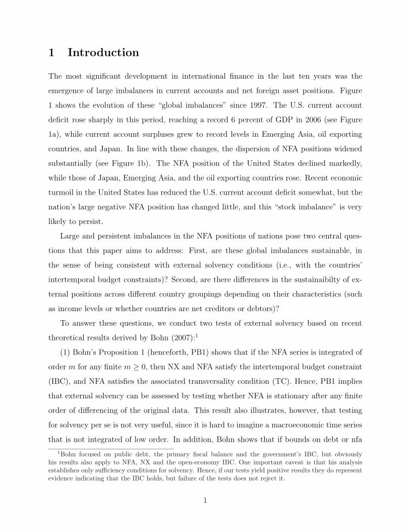
Board of Governors of the Federal Reserve System
International Finance Discussion Papers
Number 975
June 2009
On the Solvency of Nations: Are Global Imbalances Consistent with Intertemporal
Budget Constraints?
Ceyhun Bora Durdu
Enrique G. Mendoza
Marco E. Terrones
NOTE: International Finance Discussion Papers are preliminary materials circulated to stimulate discussion and critical comment. References in publications to International Finance Discussion Papers (other than an acknowledgment that the writer has had access to unpublished material) should be cleared with the author or authors. Recent IFDPs are available on the Web at www.federalreserve.gov/pubs/ifdp/. This paper can be downloaded without charge from Social Science Research Network electronic library at http://www.ssrn.com/.

On the Solvency of Nations: Are Global Imbalances Consistent with Intertemporal
Budget Constraints?
Ceyhun Bora Durdu Federal Reserve Board
Enrique G. Mendoza
University of Maryland and NBER
Marco E. Terrones International Monetary Fund
Abstract: Theory predicts that a nation's stochastic intertemporal budget constraint is satisfied if net foreign assets (NFA) are integrated of any finite order, or if net exports (NX) and NFA satisfy an error-correction specification with a residual integrated of any finite order. We test these conditions using data for 21 industrial and 29 emerging economies for the 1970-2004 period. The results show that, despite the large global imbalances of recent years, NFA and NX positions are consistent with external solvency. Country-specific unit root tests on NFA-GDP ratios suggest that nearly all of them are integrated of order 1. Pooled Mean Group error-correction estimation yields evidence of a statistically significant, negative response of the NX-GDP ratio to the NFA-GDP ratio that is largely homogeneous across countries. Keywords: global imbalances, external solvency, debt sustainability, Pooled Mean Group estimation JEL Codes: F41, F32, E66
* Author notes: We thank Shaghil Ahmed, Daniel Beltran, Betty Daniel, Linda Goldberg, David Romer, Barbara Rossi, participants of the Global Imbalances workshop at the Federal Reserve Board for comments and suggestions; Stephanie Curcuru, John Rogers for kindly sharing their data sets; Paul Eitelman, Justin Vitanza and George Zhu Yi for excellent research assistance. We also thank Gian Maria Milesi-Ferretti and Philip Lane for the data on net foreign asset positions (posted at http://www.imf.org/external/pubs/ft/wp/2006/data/wp0669.zip). The analysis undertaken in this paper would not have been possible without their efforts. All remaining errors are exclusively our responsibility. The views in this paper are solely the responsibility of the authors and should not be interpreted as reflecting the views of the International Monetary Fund, the Board of Governors of the Federal Reserve System or of any other person associated with the Federal Reserve System. Correspondence: [email protected], [email protected], [email protected].
1 Introduction
The most significant development in international finance in the last ten years was the
emergence of large imbalances in current accounts and net foreign asset positions. Figure
1 shows the evolution of these “global imbalances” since 1997. The U.S. current account
deficit rose sharply in this period, reaching a record 6 percent of GDP in 2006 (see Figure
1a), while current account surpluses grew to record levels in Emerging Asia, oil exporting
countries, and Japan. In line with these changes, the dispersion of NFA positions widened
substantially (see Figure 1b). The NFA position of the United States declined markedly,
while those of Japan, Emerging Asia, and the oil exporting countries rose. Recent economic
turmoil in the United States has reduced the U.S. current account deficit somewhat, but the
nation’s large negative NFA position has changed little, and this “stock imbalance” is very
likely to persist.
Large and persistent imbalances in the NFA positions of nations pose two central ques-
tions that this paper aims to address: First, are these global imbalances sustainable, in
the sense of being consistent with external solvency conditions (i.e., with the countries’
intertemporal budget constraints)? Second, are there differences in the sustainaibilty of ex-
ternal positions across different country groupings depending on their characteristics (such
as income levels or whether countries are net creditors or debtors)?
To answer these questions, we conduct two tests of external solvency based on recent
theoretical results derived by Bohn (2007):1
(1) Bohn’s Proposition 1 (henceforth, PB1) shows that if the NFA series is integrated of
order m for any finite m ≥ 0, then NX and NFA satisfy the intertemporal budget constraint
(IBC), and NFA satisfies the associated transversality condition (TC). Hence, PB1 implies
that external solvency can be assessed by testing whether NFA is stationary after any finite
order of differencing of the original data. This result also illustrates, however, that testing
for solvency per se is not very useful, since it is hard to imagine a macroeconomic time series
that is not integrated of low order. In addition, Bohn shows that if bounds on debt or nfa
1Bohn focused on public debt, the primary fiscal balance and the government’s IBC, but obviouslyhis results also apply to NFA, NX and the open-economy IBC. One important caveat is that his analysisestablishes only sufficiency conditions for solvency. Hence, if our tests yield positive results they do representevidence indicating that the IBC holds, but failure of the tests does not reject it.
1

exist, testing the null hypothesis of difference-stationarity seems economically uninteresting.
Because, with debt limits, m = 1 is not sufficient for sustainability. Hence, sheding light
on the characteristics of the adjustment process that sustains solvency is a more important
task, which Bohn tackled with the following result.
(2) Bohn’s Proposition 3 (henceforth, PB3) proves that if NX and NFA satisfy an error-
correction specification of the form NXt + ρNFAt−1 = zt, and zt is integrated of order m
for some ρ < 0,such that |ρ| ∈ (0, 1 + r], where r is a constant real interest rate, then the
IBC holds. This proposition implies that we can assess external solvency by estimating an
error-correction “reaction function” between NX and NFA testing for a negative, statistically
significant relationship between the two. Evidence that this reaction function exists indicates
that NX reacts in the long run to changes in NFA in such a way that NFA grows slower
than what a Ponzi scheme implies. Moreover, the magnitude of ρ drives the speed of the
adjustment process by which trade surpluses or deficits adjust to larger or smaller NFA
positions, and it becomes a key determinant of the long-run average of NFA.
We test PB1 and PB3 using a large dataset covering 51 countries during the period 1970-
2004. We test PB1 by performing standard Augmented Dickey-Fuller (ADF) and Phillips-
Perron (PP) unit root tests of the NFA-GDP ratio (nfa) using data for each individual
country separately. Then, we test PB3 by estimating an error-correction model of nfa and
the NX-GDP ratio (nx ) taking advantage of the panel dimension of the dataset. We estimate
Pesaran et. al.’s (1998) Pooled Mean Group (PMG) and Mean Group (MG) estimators, and
find strong evidence in favor of the former vis-a-vis the latter. PMG is particularly useful
in our analysis because it models the nx -nfa relationship as a long-run relationship common
to all countries in the sample, with homogeneity tests to validate this assumption (v. the
MG estimator that uses country-specific long-run relationships). Moreover, PMG allows for
country-specific short-run deviations from the long-run relationship.
The results of the unit root tests show that the hypothesis that a unit root is present in
nfa data in levels cannot be rejected for all countries in the sample. The same hypothesis
is rejected, however, for the first-difference of nfa in almost all the countries. Hence, these
results provide strong evidence in favor of the result derived in PB1. In particular, nfa is
integrated of order 1 in most countries in our sample, and therefore the IBC and TC hold.
2

Our finding that in most countries nfa ∼ I(1) implies that both IBC and TC are satisfied,
but it does not show how nx adjusts over time so that its expected present value matches the
initial nfa position, and it does not let us identify whether there are differences in the nature
of this adjustment across countries with different characteristics. The PMG estimation aims
to fill these gaps.
The PMG results show that there is a statistically significant error-correction relation
between nx and nfa both for the full sample of countries and for sub-samples separating
emerging from industrial countries, and creditor from debtor countries. The systematic long-
run component of nx responds negatively to movements in nfa, in line with Bohn’s PB3,
and homogeneity tests cannot reject the hypothesis that this component is similar across
countries (v. the null of country-specific components produced by MG estimation).
The long-run response coefficient is estimated at −0.07, which indicates that a one per-
centage point drop in nfa leads to a 0.07 percentage points increase in nx in the long run.
This result also implies that, assuming realistic growth-adjusted real interest rates (below
7 percent), both nx and nfa are stationary processes.2 The error correction coefficient is
estimated at 0.31, which implies that the adjustment of nx to a given change in nfa has an
average half-life of over 1.5 years.
The PMG results also show that nx is more responsive to movements in nfa in emerging
markets than in industrial countries. The response coefficient is 1.6 times larger in the former
than in the latter. Keeping other factors constant (i.e. country-specific fixed effects), this
difference implies that industrial countries converge to lower long-run averages of nfa that
are consistent with external solvency.
Our work is related to the large empirical literature on tests of fiscal and external solvency.
Studies include Mendoza and Ostry (2008), Trehan and Walsh (1991), Wickens and Uctum
(1993), Ahmed and Rogers (1995), Liu and Tanner (1996), Wu (2000), Wu, Show-Lin and Lee
(2001), Engel and Rogers (2006), and Nason and Rogers (2006). The tests we conduct differ
from several of the tests conducted in this literature, and in the related literature testing
2This evidence is contrary to the country-specific unit root tests that suggested that nx and nfa are notstationary. The difference in results is due to the small-sample problems of unit root tests, and to the factthat the unit root tests are country specific, while PMG estimation uses the full panel dataset to identifythe error-correction relationship.
3

for fiscal solvency, which (with the exception of Mendoza and Ostry) generally test for unit
roots in the foreign debt-GDP (or public debt-GDP) and NX-GDP (or primary balance-
GDP) ratios; for cointegration between exports and imports (or between fiscal revenues and
outlays); or for specific orders of integration in debt (public or external). Bohn (1998, 2005,
2007) showed that failure of these tests cannot be relied on to evaluate solvency because the
tests consider only sufficiency conditions that are not necessary for the IBC to hold, and
hence can indicate that observed debt dynamics violate solvency, when in fact they do not.
Our tests are in line with the literature on fiscal reaction functions pioneered by Bohn
(1998) with an application to U.S. data, and extended to a cross-country fiscal panel by
Mendoza and Ostry (2008).3 However, these reaction functions were estimated using fiscal
datasets in which public debt and fiscal balances are stationary as shares of GDP. In contrast,
the hypothesis of unit roots cannot be rejected in our external accounts data (in levels
or in shares of GDP), and hence we cannot implement Bohn’s (1998) reaction function
specification for stationary variables. Instead, we use the more general error-correction
formulation characterized in PB3, which applies even when the relevant debt stock and
net revenue flow variables are not stationary, and we also conduct the mth -order-difference
stationarity tests implied by PB1.
Our work is also related to the large and growing literature on global imbalances. This
literature presents opposing views about the sustainability of the global imbalances, along
with explanations of why the observed NFA dynamics may be consistent or inconsistent
with solvency considerations.4 In this context, the results of our work suggest that global
imbalances are consistent with external solvency. In fact, this can be the case even if nfa is
3Engel and Rogers (2006) tested for external solvency in the United States using Bohn’s (1998) test.They estimated a conditional linear reaction function for nx and the negative of the net external financialposition-to-GDP ratio over the 1791-2004 period. They obtained a negative and statistically significantresponse coefficient, which indicates failure of the sufficiency condition for external solvency.
4One group of studies (e.g., Summers(2004), Obstfeld and Rogoff (2004), Roubini and Setser (2005),Blanchard, Giavazzi and Sa (2005), Krugman (2006)) argues that these imbalances are not sustainable. Onthe other hand, other studies (e.g., Backus, Henriksen, Lambert and Telmer (2005), Bernanke (2005), Croke,Kamin and Leduc (2005), Durdu, Mendoza and Terrones (2008), Gourinchas and Rey (2005), Hausmann andSturzenegger (2005), Henriksen (2005), Mendoza, Quadrini and Rios-Rull (2007), Lane and Milesi-Ferretti(2005), Caballero, Farhi and Gourinchas (2006), Cavallo and Tille (2006), Engel and Rogers (2006), Fogliand Perri (2006), Ghironi, Lee and Rebucci (2006)), argue that the imbalances are an equilibrium outcomeof various developments such as differences in business cycle volatility, financial development, demographicdynamics, a ‘global savings glut,’ self insurance against financial crises, or valuation effects.
4

not stationary, but as long as the growth of nfa and the predicted response of nx is such
that net foreign liabilities grow at a slower pace than the one implied by a Ponzi scheme.
The rest of the paper is organized as follows: Section 2 describes the analytical foun-
dations of our empirical methodology. Section 3 presents the results of the empirical tests.
Section 4 concludes.
2 Methodology
Our methodology for testing external solvency adapts Bohn’s (2007) theoretical findings
to an open-economy environment. Consider an open economy with the following standard
period-by-period resource constraint:
NFAt = Xt −Mt + (1 + rt)NFAt−1, (1)
where M denotes imports, X exports, and r the interest rate on external assets and liabilities.
These variables could be expressed in nominal terms, real terms, or as a ratio to GDP as
long as r is adjusted accordingly (i.e., if the variables are in nominal terms, r is the nominal
interest rate; if the variables are in real terms, r is the real interest rate; if the variables are
ratios to GDP, 1 + r is the growth-adjusted real interest rate that follows from dividing the
gross real interest rate by the gross rate of output growth).
Under alternative standard simplifying assumptions about the nature of the rt process,
the resource constraint implies:5
NFAt = −ψEt[Xt+1 −Mt+1 −NFAt+1], (2)
where ψ = 1/(1 + r) < 1, and r = E[rt+1]. The above expectational difference equation,
together with this TC,
limn→∞
ψnEt[NFAt+n] = 0, (3)
5Three of these assumptions reviewed in Bohn (2007) are: (1) r positive and constant, (2) r i.i.d with apositive and constant conditional expectation, or (3) r is any stationary stochastic process with mean r > 0,and subject to implicit restrictions that may be required so that the process of “interest adjusted imports”(M∗
t = Mt − (rt − r)NFAt−1) has similar statistical properties as Mt.
5
implies the following IBC:
NFAt = −∞∑
t=1
ψiEt(Xt+i −Mt+i). (4)
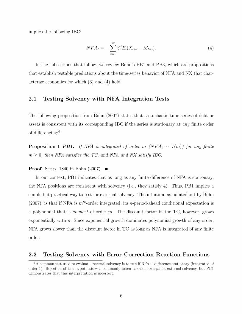
In the subsections that follow, we review Bohn’s PB1 and PB3, which are propositions
that establish testable predictions about the time-series behavior of NFA and NX that char-
acterize economies for which (3) and (4) hold.
2.1 Testing Solvency with NFA Integration Tests
The following proposition from Bohn (2007) states that a stochastic time series of debt or
assets is consistent with its corresponding IBC if the series is stationary at any finite order
of differencing:6
Proposition 1 PB1. If NFA is integrated of order m (NFAt ∼ I(m)) for any finite
m ≥ 0, then NFA satisfies the TC, and NFA and NX satisfy IBC.
Proof. See p. 1840 in Bohn (2007).
In our context, PB1 indicates that as long as any finite difference of NFA is stationary,
the NFA positions are consistent with solvency (i.e., they satisfy 4). Thus, PB1 implies a
simple but practical way to test for external solvency. The intuition, as pointed out by Bohn
(2007), is that if NFA is mth-order integrated, its n-period-ahead conditional expectation is
a polynomial that is at most of order m. The discount factor in the TC, however, grows
exponentially with n. Since exponential growth dominates polynomial growth of any order,
NFA grows slower than the discount factor in TC as long as NFA is integrated of any finite
order.
2.2 Testing Solvency with Error-Correction Reaction Functions
6A common test used to evaluate external solvency is to test if NFA is difference-stationary (integrated oforder 1). Rejection of this hypothesis was commonly taken as evidence against external solvency, but PB1demonstrates that this interpretation is incorrect.
6

Our second test of external solvency looks for a systematic negative response of NX to NFA
in the form of an error-correction specification. In particular, Bohn (2007) established the
following result:
Proposition 2 PB3. If NXt − ρNFAt−1 = zt ∼ I(m) for some ρ < 0,such that |ρ| ∈(0, 1 + r], and rt = r is constant, then NFA satisfies TC.
Proof. See p. 1844 in Bohn (2007).
This proposition states that if a country’s NX and NFA positions are linked through an
error-correction relationship with a ρ coefficient that satisfies the stated conditions, then TC
and IBC hold. Existence of such reaction function implies that, implicitly, households, firms
and the government adjust their savings and investment plans over time in a manner that is
in line with the financing requirements implied by changes in the economy’s NFA position.
With this response in place, the economy’s external liabilities grow at a slower pace than
what a Ponzi scheme implies, so that external positions are consistent with the IBC. For
countries with more negative ρ, the response of net exports to changes in net foreign assets
is stronger. In turn, more negative ρ’s are likely to reflect limitations affecting the financial
markets that those countries can access, in terms of the level of financial development and/or
the presence of financial frictions.
Efficient estimation of country-specific error-correction reaction functions linking NFA
and NX requires large data sets that are generally not available for a large number of coun-
tries. The best data available for NFA positions, which is the dataset constructed by Lane
and Milesi-Ferretti (2006), covers only the 1970-2004 period. The alternative, therefore, is
to exploit the cross-sectional, time-series structure of the data to estimate a panel error-
correction specification of the following form:
nxit − ρnfait−1 = ηit, (5)
where η is an I(0) process. This is an error-correction specification in the class of those
allowed by PB3.
Following Pesaran et al. (1999), we can nest the above relationship in an auto-regressive
distributed lag (ARDL) model in which dependent and independent variables enter the
7

right-hand-side of the model with lags of order p and q, respectively:
nxi,t = µi +
p∑j=1
λi,jnxi,t−j +
q∑
l=0
δ′i,lnfai,t−l + εi,t, (6)
where nxi,t and nfai,t denote the net exports-GDP and NFA-GDP ratios in country i at time
t respectively, and µi denotes country-specific fixed effects. ε is a set of normally distributed
error terms with country-specific variances, var(εit) = σ2i .
The above equation can be expressed in terms of a linear combination of variables in
levels and first differences, as follows:
∆nxi,t = µi + φinxi,t−1 + ϕinfai,t +
p−1∑j=1
λ∗i,j∆nxi,t−j +
q−1∑
l=0
δ∗i,l∆nfai,t−l + εi,t,
where φi = −(1 − ∑pj=1 λi,h), ϕi =
∑pj=0 δi,j, λ∗i,j = −∑p
m=j+1 λi,m, δ∗i,l = −∑qm=l+1 δi,m,
with j = 1, 2, ..., p− 1, and l = 1, 2, ..., q − 1.
To highlight the long-run relationship, the above equation can be rearranged as:
∆nxi,t = µi + φi[nxi,t−1 − ρinfai,t] +
p−1∑j=1
λ∗i,j∆nxi,t−j +
q−1∑
l=0
δ∗i,l∆nfai,t−l + εi,t, (7)
where ρi = −φ−1i ϕi denotes the long-run relationship between nx and nfa, and φi denotes
the speed at which NX adjusts towards the long-run relationship following a change in NFA.
A negative and statistically significant ρ is sufficient to guarantee that IBC in eq. (4) holds.
We estimate the dynamic panel equation (7) using MG and PMG estimators. MG es-
timates independent error-correction equations for each country and computes the mean of
the country-specific error-correction coefficients and its relevant statistics (see Pesaran and
Smith (1995)). This approach produces consistent estimates of the average of the coefficients
as long as the country-specific coefficients are independently distributed and the regressors
are exogenous. If some of the coefficients are the same for all countries, however, the MG
estimates are inefficient. In this case, PMG is efficient (see, Pesaran, et al (1999)). The
PMG estimator imposes the restriction that the long-run coefficients are the same across
countries, but the intercept, short-term coefficients and error variances can differ. The crite-
8

rion for choosing whether the PMG estimator is preferred to the MG estimator is a standard
Hausman test on the homogeneity restriction that the long-run coefficient is the same for all
countries (see Pesaran et al. (1999)).
Using the results from PMG or MG estimation, we can derive estimates of the long-run
average nfa positions to which each country converges. For the long-run average of nfa
to exist, nfa must be stationary, and this requires that the estimation results satisfy three
conditions: φ < 0, ρ < 0 and |ρ| > r. The first condition is required for the error-correction
specification to be well-defined, and the last two follow from PB3. Note that if ρ < 0 but
|ρ| ≤ r, PB3 still holds, but nfa and nx are not stationary (see Bohn (2007)).
If nfa is stationary, equation (7) and the resource constraint imply that each country’s
nfa position converges to the following long-run average:
E[nfai] =µi
φi (ρi + r). (8)
Using our PMG results, ρi is the same for all countries in the estimation panel, but there
can still be significant heterogeneity in the predicted values of E[nfai] because the estimator
still allows for country-specific estimates of φi and µi.
Since the stationarity conditions imply φi < 0 and (ρi + r) < 0, the denominator of the
right-hand-side of the above expression is positive, and therefore sign(E[nfai]) = sign(µi).
The intuition for this result is straightforward: if µi is positive (negative), the country’s
long-run trade balance converges to a deficit (surplus), and the resource constraint dictates
that in the long run E[nfai] = −E[nxi]/r (i.e., net foreign assets are equal to the negative
of the annuity value of the trade balance).
It is important to note that sign(µi) also determines whether E[nfai] is a positive or neg-
ative function of the parameters that determine it. E[nfai] is a positive (negative) function
of ρi, φi or r if µi is positive (negative). This result has an important implication: everything
else constant, countries with lower ρ converge to higher (lower) mean nfa positions if µi is
negative (positive). This result is also intuitive. Comparing two net debtor countries (each
with µi < 0), the one with a stronger response coefficient responds to temporary declines in
its nfa by adjusting its trade surplus relatively more, vis-a-vis the alternative of widening
9

more the current account deficit, and the larger surpluses imply a higher (less negative)
long-run average of nfa. A similar intuition applies to a comparison of two creditor coun-
tries. This suggests that stronger response coefficients can be viewed as evidence that the
corresponding countries have more limited access to financial markets, either to borrow or
to save, than those that display weaker response coefficients.
2.3 General Equilibrium Representation
The derivation of the IBC eq. (4) followed from a generic setup that applies to a variety
of intertemporal open-economy models, as long as TC, and the assumptions about the r
process that support the expectational difference equation for NFAt hold. The latter can
be particularly restrictive, however, because they effectively imply that the expected future
stream of trade balances in the right-hand-side of (4) can be discounted at a time- and
state-invariant average interest rate. This simplification is very useful for the proofs of PB1
and PB3, but it is important to note that the key implications of these propositions still
hold in more general environments that do not restrict discount rates in the same way. In
particular, we show below that this the case in a canonical general equilibrium model of a
small open economy with complete markets of state contingent claims traded at exogenous
world-determined prices.
Domestic output (y) in this economy is an exogenous random process, and there are
similar processes driving the output of a large number of identical countries. The world-
wide state of nature s (i.e., the vector of all country output realizations) follows a stochastic
process with the Markov transition density function f(st+1, st). Since agents have access to
complete international markets of state-contingent claims bt(st+1), the small open economy’s
period-by-period budget constraint is:
∫Q1(st+1|st)bt(st+1)dst+1 = bt−1(st) + y(st)− c(st), (9)
where Q1(st+1|st) is the period-t world-determined price of a state-contingent claim that
pays one unit of good in state st+1 at period t + 1. At equilibrium, these prices are equal
to the corresponding stochastic marginal rates of substitution in consumption across time
10

and states of nature. Given these prices, and if the appropriate TC holds, the above budget
constraint implies the following IBC:
bt−1(st) = NXt +∞∑
j=1
Et
[βju′(yt+j −NXt+j)
u′(yt −NXt)NXt+j
], (10)
where u′(·) denotes the marginal utility of consumption, β denotes the subjective discount
factor, andβju′(yt+j−NXt+j)
u′(yt−NXt)is the stochastic discount factor. If we denote by Rjt the rate of
return of a j-period-ahead risk-free asset, we can rewrite the IBC as follows:7
bt−1(st) = NXt +∞∑
j=1
{[Rjt]
−1Et(NXt+j) + covt
[βju′(yt+j −NXt+j)
u′(yt −NXt), NXt+j
]}. (11)
If the economy’s output process represents purely diversifiable country-specific risk (e.g.,
if the country-specific output processes are i.i.d. and aggregate into a non-stochastic world-
wide income), domestic agents would attain a perfectly smooth consumption path constant
across time and states, and the compounded risk-free rate would be [Rjt]−1 = βj. In this
case, the small open economy’s IBC simplifies to the same expression in (4), and propositions
PB1 and PB3 obviously apply.
If domestic agents cannot attain perfectly smooth consumption (which could happen for
a variety of reasons, such as a global component in country output fluctuations, the existence
of nontradable goods, country-specific government purchases, incomplete markets, etc.), the
expressions of the IBC in (4) and (11) are not equivalent. In particular, the co-variance
terms in the right-hand side of (11) are not zero, and as a result a constant discount factor
equal to the unconditional expectation of the interest rate, as assumed in (4), is not the
appropriate discount factor that is consistent with the true solvency condition (11). The
correct discount factor is given by the equilibrium asset pricing kernel.
The intuition for why the risk-free rate is not the appropriate discount factor is that,
depending on the shocks hitting the economy, the NFA stocks that result from the resource
7At equilibrium, this interest rate satisfies [Rjt]−1 = βjEt
[u′(yt+j−NXt+j)
u′(yt−NXt)
]
11

constraint can vary over a wide range and be correlated with sources of risk such as terms-
of-trade shocks, foreign demand shocks, etc. As a result, NFA, NX, and asset prices and
returns implied by the equilibrium pricing kernel are likely to follow very different stochastic
processes, and therefore risk-free interest rates are not appropriate discount rates for the
relevant TC. As Bohn (2005) puts it: “not just technically wrong, but also providing a
misleading economic intuition.”
Eq. (11) also implies an interesting relationship between the economy’s initial NFA
position and the sequence of conditional covariances of stochastic discount factors and NX.
In particular, given the same expected present discounted value of net exports, a Country
A with lower covariances than a Country B should display a lower initial NFA position. In
turn, assuming a standard isoelastic utility function, the covariances can be re-interpreted
as covariances between inverse consumption growth rates and net exports, which can then
be related to observed co-movements between these variables (see Section 3.2 below).
A second important implication of eq. (11) is that, as Bohn (1995 and 2005) showed,
it again implies that a reaction function with a negative, linear response of NX to NFA
is sufficient to guarantee that external solvency holds. Thus, this sufficiency condition for
solvency holds here even with an interest rate that is generally not time- and state-invariant
as assumed in PB3.
3 Estimation Results
3.1 Data
Our analysis is based on annual data for the period 1970-2004 covering 21 industrial countries
(IC) and 29 emerging markets (EM). The IC mainly comprise the core OECD countries while
the EM are those listed in Appendix 1. NFA data in U.S. dollars are from Lane and Milessi-
Feretti (2006). Data for NX and GDP in U.S. dollars are from the International Monetary
Fund’s International Financial Statistics.8 Our sample selection is simply based on data
quality and availability. The sample includes all the countries for which NFA and NX data
8Summary statistics are provided in Table 1.
12
start on or before 1990. Overall, the sample consists of 1742 observations for both the NX
and NFA positions–of which 733 observations correspond to IC group and 1009 observations
to EM group.
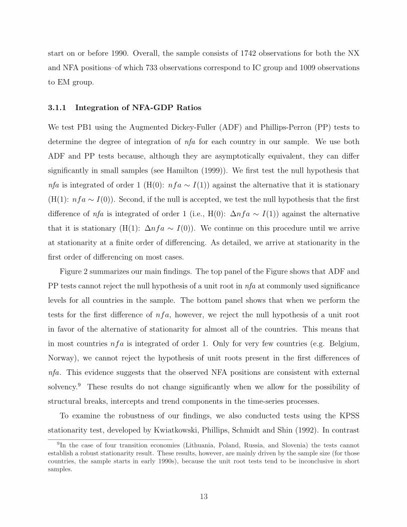
3.1.1 Integration of NFA-GDP Ratios
We test PB1 using the Augmented Dickey-Fuller (ADF) and Phillips-Perron (PP) tests to
determine the degree of integration of nfa for each country in our sample. We use both
ADF and PP tests because, although they are asymptotically equivalent, they can differ
significantly in small samples (see Hamilton (1999)). We first test the null hypothesis that
nfa is integrated of order 1 (H(0): nfa ∼ I(1)) against the alternative that it is stationary
(H(1): nfa ∼ I(0)). Second, if the null is accepted, we test the null hypothesis that the first
difference of nfa is integrated of order 1 (i.e., H(0): ∆nfa ∼ I(1)) against the alternative
that it is stationary (H(1): ∆nfa ∼ I(0)). We continue on this procedure until we arrive
at stationarity at a finite order of differencing. As detailed, we arrive at stationarity in the
first order of differencing on most cases.
Figure 2 summarizes our main findings. The top panel of the Figure shows that ADF and
PP tests cannot reject the null hypothesis of a unit root in nfa at commonly used significance
levels for all countries in the sample. The bottom panel shows that when we perform the
tests for the first difference of nfa, however, we reject the null hypothesis of a unit root
in favor of the alternative of stationarity for almost all of the countries. This means that
in most countries nfa is integrated of order 1. Only for very few countries (e.g. Belgium,
Norway), we cannot reject the hypothesis of unit roots present in the first differences of
nfa. This evidence suggests that the observed NFA positions are consistent with external
solvency.9 These results do not change significantly when we allow for the possibility of
structural breaks, intercepts and trend components in the time-series processes.
To examine the robustness of our findings, we also conducted tests using the KPSS
stationarity test, developed by Kwiatkowski, Phillips, Schmidt and Shin (1992). In contrast
9In the case of four transition economies (Lithuania, Poland, Russia, and Slovenia) the tests cannotestablish a robust stationarity result. These results, however, are mainly driven by the sample size (for thosecountries, the sample starts in early 1990s), because the unit root tests tend to be inconclusive in shortsamples.
13

with the ADF and PP unit root tests, KPSS tests the null that nfa is stationary (H(0):
nfa ∼ I(0))) against the alternative that it is integrated of order 1 (H(1): nfa ∼ I(1))). In
the event the null hypothesis is rejected, we next proceed to check if the first difference of
nfa is stationary (i.e., H(0): ∆nfa ∼ I(0)) against the alternative that it is integrated of
order 1 (H(1): ∆nfa ∼ I(1)). As in the case of the ADF and PP tests, the results of the
KPPS test indicate that nfa is integrated of finite order.10
We also performed additional robustness tests particularly for the U.S. The U.S. has
a large weight in our analysis because of its large share of global imbalances. For this
exercise, we performed the aforementioned unit root tests using a long time series data of
nfa covering 1790-2004 from Engel and Rogers (2005), and data from Curcuru et al. (2008),
which is corrected for valuation changes.11 We find that our main findings are preserved in
both datasets, i.e., nfa is nonstationary in levels but stationary in first differences.
It is important to keep in mind that the usual caveats about inference problems in short
samples due to limited power of the tests are relevant for the remainder of our sample. In
particular, it is well known that the ADF and PP tests do not have the power to distinguish
between a unit root or a near unit root process or between a drifting or trend stationary
process. In fact, when we examine the individual AR(1) coefficients for each country (see
Figure 3), we find that they span a wide range from 0.59 to 1.06, and that their standard
errors are relatively large (ranging from 0.065 to 0.146). Thus, although we could not reject
the hypothesis of unit roots in nfa, the possibility remains that due to the low power of the
tests the true data generating process is in fact stationary in levels. This, however, would
not affect our finding that the data support the hypothesis that the solvency condition holds,
since stationarity in levels is also consistent with PB1.
3.1.2 Panel Error-Correction Estimation
We test PB3 by estimating the dynamic panel equation derived in the previous Section using
PMG and MG estimators. Table 2 reports results for the full sample combining ICs and
EMs and subsamples separating ICs from EMs. The table is divided in two blocks. Block
10The results for KPSS tests are available upon requests.11We thank corresponding authors for kindly sharing their dataset.
14

1 shows our baseline results, and Block 2 shows results obtained with the data expressed
as ratios of world gdp.12 The ARDL lag structure for each country was selected using
the Schwartz Bayesian criterion. For the majority of countries, specifications without lagged
dependent variables are rejected at conventional levels of statistical significance. Throughout
this section, we examine the null hypothesis that there is no error-correction relation between
nfa and nx under both the PMG and MG estimators, and use t-statistics to test this
hypothesis.
The Full Sample panel in Block 1 of Table 2 shows the main results combining all the
countries in our sample. The Hausmann h-statistic test cannot reject the slope homogeneity
restriction, indicating that the PMG estimator is preferred to the MG estimator. The PMG
estimates of the long-run response coefficient show a negative and statistically signficant
response of nx to nfa. A reduction (increase) of one percentage point in nfa rises (lowers)
nx by 0.07 percentage points. The estimated error correction coefficient of 0.31 (in absolute
value) indicates that the adjustment of nx to a given change in nfa has an average half-life
of just over 1.75 years. Overall, these results for the full sample indicate that PB3 and the
external solvency conditions hold.
The IC and EM panels of Block 1 in Table 2 show that the results of MG and PMG
estimation splitting the sample according to whether countries are industrialized or emerging
economies also support the hypothesis that PB3 holds. The null hypothesis of no error-
correction relation between nx and nfa is rejected in both the IC and EM groups. The h-test
indicates that PMG dominates MG for both the IC and EM groups. Comparing across the
two groups, we find that the long-run response coefficient is higher in EMs than in ICs (-0.085
v. -0.053). Both of these estimates are statistically significant at a 5 percent significance
level. The error-correction coefficients imply that the adjustment of nx to changes in nfa
is more protracted in ICs, for which the average half-life is about 2.8 years, than in EM, for
which the average half-life is 112
years.13
The result indicating that the long-run response coefficient of EMs is about 1.6 times
12We also studied the results where only those countries with statistically significant EC coefficients, andintercept terms (as reported in Table 3) are kept in the sample. We found that the results are robust to thesample selection.
13The half-life is calculated as log(0.5)/ log(1− |EC|), where EC denotes the error correction coefficient.The higher is the |EC|, the lower is the half-life and the faster is the adjustment.
15

larger than that for ICs implies that net exports in EMs need to respond more to changes in
net foreign assets in order to support external solvency. As suggested earlier, this difference
can be attributed to the underdevelopment of financial markets or the severity of the financial
frictions that EMs face compared to ICs.
Table 3 shows the long-run nfa positions that each country converges to. In this table,
we report the estimates for only those countries with statistically significant EC coefficient
(phi) and intercept (mu). The nfa estimates reported in column 5 are calculated using the
formula in (8). The column labeled “nfa for constant mu” calculates the implied estimate for
nfa in the formula where the intercept term (mu) is set to the value estimated for the whole
sample (All). The purpose of this exercise is to illustrate the potential changes in estimated
nfa driven solely by the changes in the EC term (phi). Likewise, the last column shows the
estimates for nfa when the EC coefficient is fixed at the estimate for the whole sample to
illustrate the importance of the intercept term (mu). The main lesson we derive from this
exercise is that although the long-run coefficient (rho) is kept the same, there are marked
variations in long-run nfa estimates that each country converges to. The large changes in
these estimates are driven by differences in the EC and intercept terms, which, in turn, is
affected by the structural differences across countries.
Figures 4a-b illustrate the impulse responses functions of nfa and nx when the economy
is subject to a one-standard-deviation noise shock (figures are shown for only a selected
set of countries reported in Table 3 due to space limitations). These impulse responses are
calculated using the PMG estimates reported in Tables 4, and setting the initial nfa and nx
positions to their long-run values that they converge to. The main finding is that although
nx can converge back to its long-run equilibrium faster, the adjustment of nfa (i.e., the stock
imbalance) can persist much longer. The convergence of the nfa positions to their long-run
values in our sample takes from about 10 years up to 50 years. Our exercise also illustrate
that although the long-run coefficients are common across EMs and ICs, there is marked
variation among countries in their convergence. This exercise affirms that the framework
preserves the heterogeneity across countries on how they respond to similar shocks. This
heterogeneity arises due to structural differences among these countries as mentioned earlier.
16

3.2 Robustness
We study next the robustness of our results to the representation of the data. To do so,
we study how our results change when we use an alternative representation of the data in
which the NX and NFA series are normalized using world GDP instead of country-specific
GDPs (Block 2, Table 2). In the latter exercise, the world GDP is simply the sum of the
respective GDPs of the countries in the sample, each expressed in U.S. dollars. The purpose
of this exercise is to explore if the baseline results are altered by relative country size and
by restrictions that force global market clearing.
In Block 2, the results for the Full Sample panel show that again the Hausman h-test
indicates that the cross-country slope homogeneity restriction cannot be rejected, albeit
marginally, and that the PMG estimate of the response coefficient (−0.08) must be chosen
over the MG estimator. Moreover, the average half-life of adjustment to the long-run rela-
tionship in this scenario is 134
years. These results are very similar to those obtained using
the standard nx and nfa measures based on country GDPs.
The results for the IC panel with world gdp ratios are also similar to those obtained
with country gdp ratios, but the results for the EM panel are different. The Hausmann h-
test cannot reject the long-run homogeneity condition for ICs, which implies that the PMG
estimate of −0.057 is preferred to the MG estimator. In addition, the average half life for this
country group is 2.6 years. Both of these estimates are very similar to those reported using
country gdp ratios. For EMs, however, the Hausmann h-test suggests that the hypothesis
of long-run homogeneity should be rejected and that the MG estimate of −0.235 should be
chosen. This estimate is almost 3 times larger than the one reported earlier. In contrast,
the average half-life is estimated at 1.2 years, which is slightly lower than the one reported
earlier.
The next robustness test explores the implications of splitting the sample into creditor
countries (also called “High NFA” countries) and debtor (“Low NFA”) countries. Creditor
(debtor) countries are defined as those with above (below) median nfa using each country’s
GDP.14 The results of the dynamic panel estimation are shown in Panel 1 of Table 4. For
creditors, the Hausmann h-test cannot reject the cross-country homogeneity restriction and,
14The list of countries pertaining to each group is available on request.
17

thus, indicates that the PMG estimate of −0.095 should be preferred. The average half-life
for this group is estimated at 1.94 years. For debtors, the Hausmann h-test indicates that
the cross-country homogeneity restriction cannot be rejected and that the PMG estimate of
−0.061 is preferred. The average half-life for this group of countries is estimated at 1.6 years.
In summary, these findings suggest that in terms of its implications for sustainability, there
is no significant behavioral difference between creditor and debtor countries. However, in
terms of long-run nfa positions these countries converge to creditor countries will converge
to higher nfa positions than debtor countries in the long-run.
Next, we explore the importance of trade openness (panel 2, Table 4). Those countries
with a volume of trade as a share of GDP higher than the volume for the median country
are treated as more open economies, and the rest is treated as less open economies. For
both groups, the long-run homogeneity restriction cannot be rejected. The implied PMG
estimates are −0.070 (with half life 2.2 years) and −0.065 (with half life 1.4 years) for more
open and less open economies, respectively, suggesting that there is no significant difference
between these two groups.
We also explore the importance of institutional quality, financial sector development,
and capital account openness as shown in panels 3-5, respectively. In all these cases, Haus-
mann test cannot reject the long-run homogeneity restriction so that the PMG should be
the preferred method. These results mainly show that the countries with relatively weaker
fundamentals (i.e., less institutional quality, less financial sector development, and less open
to capital) need to respond more strongly to the changes in NFA to keep them on a sustain-
able path (notice that implied PMG estimates for the long-run coefficient is more negative
for these groups compared to their counterparts with stronger fundamentals). However, our
baseline findings regarding the sustainability of imbalances are preserved in all these cases.
4 Conclusion
This paper explored whether external solvency conditions hold in existing cross-country data
on trade balances and net foreign assets, which largely reflects the recent episode of large and
growing global imbalances. We conducted external solvency tests for a panel of 21 industrial
18

and 30 emerging market countries during the 1970-2004 period.
Our solvency tests are based on two propositions postulated by Bohn (2007). The first
proposition shows that solvency is satisfied if NFA are integrated of any finite order. When
we tested this proposition, we found that we could not reject the presence of unit roots in
nfa in levels in all of the countries in our sample, but that unit roots are rejected for the
first-differences of nfa in virtually all the countries.
Bohn’s second proposition shows that solvency holds if NFA and NX are linked by an
error-correction reaction function. Using dynamic panel estimation methods, we found that
a statistically significant error-correction relationship between those two series does exist in
the data. In particular, we found a systematic, negative long-run response of nx to changes
in nfa. Comparing industrial and emerging countries, we found that the response coefficient
of the latter is higher, and that as a result emerging economies converge to higher long-run
averages of nfa than industrial countries.
19

References
[1] Ahmed, S. and J. H. Rogers (1995). “Government Budget Deficits and Trade Deficits:
Are Present-Value Constraints Satisfied in Long-Term Data?”, Journal of Monetary
Economics, vol. 36, pp. 351-74.
[2] Backus, D., Henriksen, E., Lambert, F., and Telmer, C. (2005). “Current Account Fact
and Fiction.” Unpublished manuscript, New York University.
[3] Bernanke, B. S. (2005). “The Global Saving Glut and the U.S. Current Account Deficit.”
Speech at the Sandridge Lecture, Virginia Association of Economists, March 10, 2005.
[4] Blanchard, O., Giavazzi, F., and Sa, F. (2005). “The U.S. Current Account and the
Dollar.” NBER Working Paper No. 11137.
[5] Bohn, H. (1998). “The Behavior of U.S. Public Debt and Deficits.” Quarterly Journal
of Economics, Vol. 113, pp. 949-63.
[6] Bohn, H. (2005). “The Sustainability of Fiscal Policy in the United States.” Mimeo,
Department of Economics, University of California-Santa Barbara.
[7] Bohn, H. (2007). “Are Stationary and Cointegration Restrictions Really Necessary for
the Intertemporal Budget Constraint?.” Journal of Monetary Economics, Vol. 54, pp.
1837-1847.
[8] Caballero, R. J., Farhi, E., and Gourinchas, P. O. (2006). “An Equilibrium Model of
“Global Imbalances” and Low Interest Rates.” American Economic Review, Vol. 98(1),
pp. 358-393.
[9] Cavallo, M. and Tille, C. (2006). “Could Capital Gains Smooth a Current Account
Rebalancing?” Federal Reserve Bank of New York Staff Report 237, January.
[10] Croke, H., Kamin, S. B., and Leduc, S. (2005). “Financial Market Developments and
Economic Activity during Current Account Adjustments in Industrial Economies.” In-
ternational Finance Discussion Papers No. 827, Board of Governors of the Federal Re-
serve System.
20

[11] Curcuru, S., T. Dvorak, and F. Warnock. (2008). “Cross Border Return Differentials.”
Quarterly Journal of Economics, Vol. 124, pp. 1495-1530, November.
[12] Durdu, C. B., E. G. Mendoza and M. E. Terrones (2008). Precautionary Demand for
Foreign Assets in Sudden Stop Economies: An Assessment of the New Merchantilism.
Journal of Development Economics, forthcoming.
[13] Engel, C. and Rogers, J.H. (2008), “The U.S. Current Account Deficit and the Expected
Share of World Output,” Journal of Monetary Economics, forthcoming.
[14] Fogli, A. and Perri, F. (2006). “The great moderation and the US external imbalance,”
mimeo, Department of Economics, University of Minnesota.
[15] Ghironi, F., J. Lee and A. Rebucci (2006), “The Valuation Channel of External Adjust-
ment,” mimeo, Research Department, International Monetary Fund.
[16] Gourinchas, P. O. and Rey, H. (2005). “From World Banker to World Venture Capitalist:
US External Adjustment and the Exorbitant Privilege.” NBER Working Paper No.
11563.
[17] Hausmann, R. and Sturzenegger, F. (2005), “U.S. and Global Imbalances: Can Dark
Matter Prevent a Big Bang?.” Center for International Development, Harvard Univer-
sity, Working Paper No. 124.
[18] Lane, P. and G. M. Milesi-Ferretti (2006). “The External Wealth of Nations Mark II:
Revised and Extended Estimates of Foreign Assets and Liabilities, 1970-2004. ” IMF
Working Paper 06/69.
[19] Henriksen, E. R. (2004), “A Demographic Explanation of U.S. and Japanese Current
Account Behvaior.” mimeo, Carnegie-Mellon University.
[20] Krugman, P. (2006), “Will there be a Dollar crisis?,” mimeo.
[21] Lane, P. R. and Milesi-Ferretti, G. M. (2005). “A Global Perspective on External Posi-
tion.” NBER Working Paper No. 11589.
21

[22] Lane, P. R. and Milesi-Ferretti, G. M. (2006). “The External Wealth of Nations Mark
II: Revised and Extended Estimates of Foreign Assets and Liabilities, 1970-2004.” IMF
Working Paper 06/69.
[23] Liu, P. and E. Tanner (1996). “International Intertemporal Solvency in Industrialized
Countries: Evidence and Implications.” Southern Economic Journal, Vol. 62. Pp. 739-
49.
[24] Mendoza, E. G. and J. Ostry (2007). “International Evidence on Fiscal Solvency: Is
Fiscal Policy “Responsible”?.” NBER Working Paper, No. 12947.
[25] Obstfeld, M. and Rogoff, K. (2004). “The Unsustainable US Current Account Position
Revisited.” NBER Working Paper No. 10869, November.
[26] Roubini, N. and Setser, B. (2005). “Will the Bretton Woods 2 Regime Unravel Soon?
The Risk of a Hard Landing in 2005-2006,” Unpublished manuscript, New York Uni-
versity and Oxford University.
[27] Summers, L. H. (2004). “The United States and the Global Adjustment Process.” Speech
at the Third Annual Stravos S. Niarchos Lecture, Institute for International Economics,
March 23, 2004.
[28] Terrones, M. E. and R. Cardarelli (2005). “Global Imbalances: A Saving and Investment
Perspective.” WEO, Building Institutions, September.
[29] Trehan, B. and Walsh, C. E. (1991). “Testing Intertemporal Budget Constraints: Theory
and Applications to U.S. Federal Budget and Current Account Deficits,” Journal of
Money, Credit and Banking, vol. 23(2), pp. 206-23, May.
22

Appendix I: Derivation of the PMG equation
Following Pesaran et al. (1999), we can nest the relationship in eq. 5 in an auto-regressive
distributed lag (ARDL) model in which dependent and independent variables enter the
right-hand-side of the model with lags of order p and q, respectively:
nxi,t = µi +
p∑j=1
λi,jnxi,t−j +
q∑
l=0
δ′i,lnfai,t−l + εi,t,
where nxi,t and nfai,t denote the net exports-GDP and NFA-GDP ratios in country i at time
t respectively, and µi denotes country-specific fixed effects. ε is a set of normally distributed
error terms with country-specific variances, var(εit) = σ2i .
Using the following identity in the left-hand side of the equation nxi,t = nxi,t−1 + ∆nxi,t;
and the following identities in the right-hand side of the equation nxi,t−1 = nxi,t − ∆nxi,t
and nfai,t−1 = nfai,t −∆nfai,t; the above equation can be rewriten as follows:
nxi,t−1 + ∆nxi,t = µi + λi,1nxi,t−1 + δi,0nfai,t +
p∑j=2
λi,j[nxi,t−j+1 −∆nxi,t−j+1]
+
q∑
l=1
δi,l[nfai,t−l+1 −∆nfai,t−l+1] + εi,t,
or
∆nxi,t = µi − (1− λi,1 − λi,2...)nxi,t−1 + (δi,0 + δi,1 + ...)nfai,t − (λi,2
+λi,3 + ...)∆nxi,t−1 − (λi,3 + λi,4 + ...)∆nxi,t−2 − ...
−(δi,2 + δi,3 + ...)∆nfai,t−1 − (δi,3 + δi,4 + ...)∆nfai,t−2 − ... + εi,t,
or
23

∆nxi,t = µi + φinxi,t−1 + ϕinfai,t +
p−1∑j=1
λ∗i,j∆nxi,t−j +
q−1∑
l=0
δ∗i,l∆nfai,t−l + εi,t,
where φi = −(1−∑pj=1 λi,h), ϕi =
∑pj=0 δi,j, λ∗i,j = −∑p
m=j+1 λi,m, δ∗i,l = −∑qm=l+1 δi,m,
with j = 1, 2, ..., p− 1, and l = 1, 2, ..., q − 1.
To highlight the long-run relationship, the above equation can be rearranged as:
∆nxi,t = µi + φi[nxi,t−1 − ρinfai,t] +
p−1∑j=1
λ∗i,j∆nxi,t−j +
q−1∑
l=0
δ∗i,l∆nfai,t−l + εi,t,
where ρi = −φ−1i ϕi denotes the long-run equilibrium relationship between nx and nfa,
and φi denotes the speed at which NX adjust toward their long-run equilibrium following a
change in NFA.
Appendix II: Sample of Countries
The sample comprises 21 industrial countries and 30 emerging markets.
Industrial Countries: Australia (AUS), Austria (AUT), Belgium (BEL), Canada (CAN),
Denmark (DNK), Finland (FIN), France (FRA), Germany (DEU), Greece (GRC), Ireland
(IRL), Italy (ITA), Japan (JPN), Netherlands (NLD), New Zealand (NZL), Norway (NOR),
Portugal (PRT), Spain (ESP), Sweden (SWE), Switzerland (CHE), United Kingdom (GBR),
United States (USA).
Emerging Markets: Argentina (ARG), Brazil (BRA), Chile (CHL), China (CHN),
Colombia (COL), Costa Rica (CRI), Ecuador (ECU), Egypt (EGY), El Salvador (SLV),
Hong Kong (HKG), Hungary (HUN), India (IND), Indonesia (IDN), Israel (ISR), Jordan
(JOR), Korea (KOR), Malaysia (MYS), Mexico (MEX), Morocco (MAR), Pakistan (PAK),
Peru (PER), Philippines (PHL), Saudi Arab (SAU), Singapore (SGP), South Africa (ZAF),
Thailand (THA), Turkey (TUR), Uruguay (URY), Venezuela (VEN).
24

* China, Hong Kong, Indonesia, Korea, Malaysia, Philippines, Singapore, Taiwan and Thailand.** Algeria, Angola, Azerbaijan, Bahrain, Rep. of Congo, Ecuador, Equatorial Guinea, Gabon, Iran, Kuwait, Libya, Nigeria, Norway, Oman, Qatar, Russia, Saudi Arabia, Syria, Turkmenistan, UAE, Venezuela and Yemen
Figure 1a. Current Account Balances
Figure 1b. Net Foreign Assets
-10
-5
0
5
10
15
20
1997 1998 1999 2000 2001 2002 2003 2004 2005 2006 2007
Pe
rce
nt
of
GD
P
U.S. Euro Area Japan Emerging Asia* Oil Exporters**
-30
-20
-10
0
10
20
30
40
50
60
1997 1998 1999 2000 2001 2002 2003 2004 2005 2006 2007
Pe
rce
nt
of
GD
P
U.S. Euro Area Japan Emerging Asia* Oil Exporters**

Figure 2. The Order of Intergration of Net Foreign Assets Positions
0.0
0.1
0.2
0.3
0.4
0.5
0.6
0.7
0.8
0.9
1.0
Au
stri
alia
Au
stri
aB
elgi
um
Can
ada
Den
mar
kFi
nla
nd
Fran
ceG
erm
any
Gre
ece
Irel
and
Ital
yJa
pan
Net
her
lan
ds
New
Zea
lan
dN
orw
ayP
ort
uga
lSp
ain
Swed
enSw
itze
rlan
dU
KU
S
Arg
enti
na
Bra
zil
Ch
ileC
hin
aC
olo
mb
iaC
ost
a R
ica
Ecu
ado
rEg
ypt
El S
alva
do
rH
on
g K
on
gH
un
gary
Ind
iaIn
do
nes
iaIs
rael
Jord
anK
ore
aM
alay
sia
Mex
ico
Mo
rocc
oP
akis
tan
Per
uP
hili
pp
ines
Sau
di A
rab
iaSi
nga
po
reSo
uth
Afr
ica
Thai
lan
dTu
rkey
Uru
guay
Ven
ezu
ela
p-s
tat
Lag = 1
Dickey-Fuller
Phillips-Perron
Critical Value
0
0.1
0.2
0.3
0.4
0.5
0.6
0.7
0.8
0.9
1
Au
stri
alia
Au
stri
aB
elgi
um
Can
ada
Den
mar
kFi
nla
nd
Fran
ceG
erm
any
Gre
ece
Irel
and
Ital
yJa
pan
Net
her
lan
ds
New
Zea
lan
dN
orw
ayP
ort
uga
lSp
ain
Swed
enSw
itze
rlan
dU
KU
S
Arg
enti
na
Bra
zil
Ch
ileC
hin
aC
olo
mb
iaC
ost
a R
ica
Ecu
ado
rEg
ypt
El S
alva
do
rH
on
g K
on
gH
un
gary
Ind
iaIn
do
nes
iaIs
rael
Jord
anK
ore
aM
alay
sia
Mex
ico
Mo
rocc
oP
akis
tan
Per
uP
hili
pp
ines
Sau
di A
rab
iaSi
nga
po
reSo
uth
Afr
ica
Thai
lan
dTu
rkey
Uru
guay
Ven
ezu
ela
p-s
tat
Lag = 0
Dickey-Fuller
Phillips-Perron
Critical Value

Figure 3. The Estimated AR(1) Coefficients
0
0.2
0.4
0.6
0.8
1
1.2
Au
stri
a
Be
lgiu
m
Fin
lan
d
Ge
rman
y
Gre
ece
Ne
w Z
eal
and
Swe
de
n
Swit
zerl
and
UK
US
Bra
zil
Ch
ile
Ch
ina
Co
lom
bia
Co
sta
Ric
a
Ecu
ado
r
Ho
ng
Ko
ng
Hu
nga
ry
Ind
ia
Ko
rea
Me
xico
Mo
rocc
o
Pak
ista
n
Pe
ru
Sin
gap
ore
Thai
lan
d
Turk
ey
Ve
ne
zue
la
Net Foreign Assets
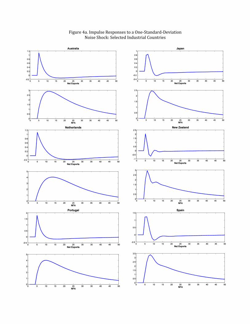
Figure 4a. Impulse Responses to a One-Standard-Deviation Noise Shock: Selected Industrial Countries

Figure 4b. Impulse Responses to a One-Standard-Deviation Noise Shock: Selected Emerging Markets

Table 1. Sample StatisticsPeriod 1970-2004
All Industrial EmergingCountries Market
Economies
1. Net exports (% of GDP)
Mean -0.872 0.182 -1.637Median -0.518 0.196 -1.380Bottom quartile -3.640 -1.910 -5.290Top quartile 2.410 2.430 2.410Standard deviation 8.367 4.640 10.192Number of observations 1742 733 1009Number of countries 50 21 29
2. Net foreign assets (% of GDP)
Mean -17.922 -9.195 -24.429Median -20.831 -10.021 -31.037Bottom quartile -40.105 -25.303 -47.638Top quartile -3.997 4.775 -13.497Standard deviation 43.021 35.082 47.071Number of observations 1716 733 983Number of countries 50 21 29

Full Sample Industrial Countries Emerging MarketsMG PMG MG PMG MG PMG
1. As a Percent of Country GDP
LR Coefficient -0.186** -0.068*** -0.243 -0.053*** -0.144*** -0.085***[0.084] [0.008] [0.194] [0.011] [0.039] [0.012]
EC Coefficient -0.357*** -0.311*** -0.284*** -0.219*** -0.409*** -0.383***[0.035] [0.037] [0.045] [0.043] [0.050] [0.052]
Hausman Statistics 1.99 0.97 2.61p-value [0.33] [0.33] [0.11]
Number of countries 50 50 21 21 29 29
2. As a Percent of World GDP^
LR Coefficient -0.491 -0.078*** -0.871 -0.056*** -0.225*** -0.093***[0.336] [0.009] [0.813] [0.013] [0.068] [0.012]
EC Coefficient -0.377*** -0.329*** -0.290*** -0.299*** -0.438*** -0.406***[0.039] [0.041] [0.048] [0.046] [0.056] [0.058]
Hausman Statistics 1.52 1.00 3.95p-value [0.22] [0.32] [0.05]
Number of countries 51 51 21 21 30 30
(1970-2004 period)Table 2. Dynamic Panel Estimates of Net Exports on Net Foreign Assets
Note: The symbols *, ** and *** indicate statistical significance at the 10%, 5% and 1%, levels, respectively. Standard errors are reported in brackets. The Hausman statistic refers to the test statistic on the long-run homogeneity restriction. The maximum number of lags considered in the estimation is 2.^Includes the Rest of the World, which is created as the negative of the global external imbalances. The World Output is the sum of the outputs of industrial and emerging market countries in our sample.

Countries rho phi mu nfanfa for
constant munfa for
constant phi
Industrial CountriesAustralia -0.053 -0.322*** -1.080** -45.961 -10.462 -67.599Japan -0.053 -0.337*** 0.685*** 27.840 -9.997 42.854Netherlands -0.053 -0.216** 1.109** 70.324 -15.587 69.425New Zealand -0.053 -0.889*** -3.386*** -52.150 -3.788 -211.816Portugal -0.053 -0.380*** -3.919*** -141.020 -8.852 -245.143Spain -0.053 -0.395*** -0.89*** -31.114 -8.529 -56.133All -0.053 -0.219*** -0.246** -15.388 -15.388 -15.388
Emerging MarketsBrazil -0.085 -0.313*** -0.748* -22.746 -33.762 -18.612Chile -0.085 -0.499*** -1.582* -30.159 -21.179 -39.341Costa Rica -0.085 -0.409*** -3.428*** -79.728 -25.839 -85.244Hong Kong -0.085 -0.117** 1.682* 136.972 -90.435 41.843Hungary -0.085 -0.324** -1.991** -58.494 -32.637 -49.514India -0.085 -0.468*** -1.320*** -26.836 -22.580 -32.834Jordan -0.085 -0.209* -6.936* -315.912 -50.602 -172.473Mexico -0.085 -0.315** -1.117* -33.747 -33.548 -27.791Morocco -0.085 -0.275*** -3.317*** -114.531 -38.351 -82.504Peru -0.085 -0.349*** -2.271** -61.974 -30.309 -56.489Philippines -0.085 -0.282** -2.456** -82.851 -37.468 -61.089All -0.085 -0.383*** -1.111** -27.627 -27.627 -27.627Note: The table shows the long-run NFA positions that the PMG model converges to for thecountries with significant phi an mu. The last two columns illustrate the respective implied NFApositions if the EC coefficient and intercept terms were kept constant at the value estimated for the whole sample.
Table 3. Long-run NFA

MG PMG MG PMG MG PMG MG PMG MG PMG MG PMG
LR Coefficient -0.285* -0.061*** -0.087** -0.095*** -0.104** -0.065*** -0.267 -0.070*** -0.224 -0.055*** -0.147*** -0.083***[0.162] [0.010] [0.039] [0.016] [0.041] [0.012] [0.163] [0.012] [0.164] [0.011] [0.041] [0.012]
EC Coefficient -0.349*** -0.315*** -0.364*** -0.300*** -0.488*** -0.404*** -0.266*** -0.218*** -0.287*** -0.226*** -0.427*** -0.403***[0.046] [0.046] [0.055] [0.059] [0.056] [0.061] [0.036] [0.033] [0.040] [0.039] [0.056] [0.058]
Hausman Statistics 1.91 0.05 0.99 1.48 1.06 2.79p-value [0.17] [0.82] [0.32] [0.22] [0.30] [0.09]
Number of countries 25 25 25 25 25 25 25 25 25 25 25 25
MG PMG MG PMG MG PMG MG PMG
LR Coefficient -0.235 -0.063*** -0.137*** -0.074*** -0.230 -0.054*** -0.141*** -0.085***[0.164] [0.011] [0.041] [0.012] [0.164] [0.011] [0.040] [0.013]
EC Coefficient -0.280*** -0.226*** -0.434*** -0.397*** -0.299*** -0.240*** -0.414*** -0.386***[0.036] [0.037] [0.058] [0.060] [0.049] [0.049] [0.049] [0.052]
Hausman Statistics 1.11 2.56 1.16 2.16p-value [0.29] [0.11] [0.28] [0.14]
Number of countries 25 25 25 25 25 25 25 25
Less Open to Capital
Note: The symbols *, ** and *** indicate statistical significance at the 10%, 5% and 1%, levels, respectively. Standard errors are reported in brackets. The Hausman statistic refers to the test statistic on the long-run homogeneity restriction. The maximum number of lags considered in the estimation is 2.
Table 4. Dynamic Panel Estimates of Net Exports on Net Foreign Assets(As percent of GDP, 1970-2004 period)
Less Institutional Quality
More Financial Sector Dev. Less Financial Sector Dev. More Open to Capital
Less Open Economies More Open Economies
4. Financial Sector Development 5. Capital Account Openness
More Institutional QualityDebtor Economies Creditor Economies1. Debtor vs. Creditor 2. Trade Openness 3. Institutional Quality