Embed Size (px)
Citation preview
arX
iv:m
ath/
0405
330v
3 [
mat
h.Q
A]
29
Oct
200
4
ON THE STRUCTURE OF COFREE HOPF ALGEBRAS 1
On the structure of cofree Hopf algebras
By Jean-Louis Loday and Marıa Ronco
Abstract
We prove an analogue of the Poincare-Birkhoff-Witt theorem and of theCartier-Milnor-Moore theorem for non-cocommutative Hopf algebras. The prim-itive part of a cofree Hopf algebra is a B∞-algebra. We construct a universalenveloping functor U2 from B∞-algebras to 2-associative algebras, i.e. algebrasequipped with two associative operations. We show that any cofree Hopf algebraH is of the form U2(PrimH). Taking advantage of the description of the free2as-algebra in terms of planar trees to unravel the structure of the operad B∞.
1. Introduction
In their celebrated paper [16] John Milnor and John Moore proved that,
over a field of characteristic zero, any connected cocommutative Hopf algebra
H is of the form U(PrimH), where the primitive part PrimH is viewed as a
Lie algebra, and U is the universal enveloping functor (See also the work of
Pierre Cartier in [4]). Combined with the Poincare-Birkhoff-Witt theorem, it
gives an equivalence between the cofree cocommutative Hopf algebras and the
Hopf algebras of the form U(g), where g is a Lie algebra.
Our aim is to prove a similar result without the assumption “cocommu-
tative” and to get a structure theorem for cofree Hopf algebras. In order to
achieve this goal we need to consider PrimH as a B∞-algebra (cf. 1.4) instead
of a Lie algebra. A B∞-algebra is defined by (p + q)-ary operations for any
pair of positive integers (p, q) satisfying some relations. This structure ap-
pears naturally in algebraic topology. The universal enveloping functor U is
replaced by a functor U2 from B∞-algebras to 2-associative algebras, which are
vector spaces equipped with two associative operations. We prove the following
Theorem. If H is a bialgebra over a field K, then the following are equivalent:
(a) H is a connected 2-associative bialgebra,
(b) H is isomorphic to U2(PrimH) as a 2-associative bialgebra,
(c) H is cofree among the connected coalgebras.
ON THE STRUCTURE OF COFREE HOPF ALGEBRAS 2
Hence, as a consequence, we get a structure theorem for cofree Hopf alge-
bras: any cofree Hopf algebra is of the form U2(R) where R is a B∞-algebra.
The notion of 2-associative bialgebra occuring in the theorem is as follows.
A 2-associative bialgebra H is a vector space equipped with two associative
operations denoted ∗ and · and a cooperation ∆. We suppose that (H, ∗,∆) is
a bialgebra (in the classical sense), and that (H, ·,∆) is a unital infinitesimal
bialgebra. The difference with the classical notion is in the compatibility rela-
tion between the product and the coproduct which, in the unital infinitesimal
case, is
∆(x · y) = (x⊗ 1) ·∆(y) + ∆(x) · (1⊗ y)− x⊗ y .
The following structure theorem for unital infinitesimal bialgebras is the key
result in the proof of the main theorem.
Theorem. Any connected unital infinitesimal bialgebra is isomorphic to the
tensor algebra (i.e. non-commutative polynomials) equipped with the deconcate-
nation coproduct.
Observe that, in our main theorem, (a) ⇒ (b) is the analogue of the
Cartier-Milnor-Moore theorem (cf. [4], [16]), that (b) ⇒ (c) is the analogue of
the Poincare-Birkhoff-Witt theorem, and that (a) ⇒ (c) is the analogue of a
theorem of Leray in the cocommutative case.
The universal enveloping 2as-algebra U2(R), where R is a B∞-algebra, is
a quotient of the free 2as-algebra 2as(V ) for V = R. So it is important to know
an explicit description of 2as(V ) for any vector space V . We show that, as an
associative algebra for the product ∗, 2as(V ) is the non-commutative polyno-
mial algebra (i.e. tensor algebra) over the planar rooted trees. We describe the
other product · and the coproduct ∆ in terms of trees. This description is very
similar to the description of the Hopf algebra of (non-planar) rooted trees given
by Connes and Kreimer (cf. [5]). Here the rooted trees are replaced by the
planar rooted trees, and the polynomials by the non-commutative polynomials.
The free Lie algebra is a complicated object which is mainly studied
through its embedding in the free associative algebra, that is its identifica-
tion with the primitive part of the tensor algebra. The free B∞-algebra is, a
priori, an even more complicated object (it is generated by k-ary operations
for all k). Our main theorem permits us to identify it with the primitive part
of the free 2-associative algebra. Since we can describe explicitly the free 2-
associative algebra in terms of trees, we can prove the following
Corollary. The operad B∞ of B∞-algebras is such that B∞(n) = K[TTn] ⊗
K[Sn], where TTn is the set of planar rooted trees with n leaves, and Sn is the
symmetric group.
ON THE STRUCTURE OF COFREE HOPF ALGEBRAS 3
The content of this paper is as follows. In section 2 we recall the classical
notion of bialgebras and B∞-algebras. In section 3, which can be read indepen-
dently of section 2, we recall the notion of unital infinitesimal bialgebra and we
prove the key result which says that there is only one kind of connected unital
infinitesimal bialgebra. In section 4 we introduce the notion of 2-associative
algebra and 2-associative bialgebra, and we construct the universal enveloping
functor U2. In section 5 we state and prove the main theorem. Our proof
is based on the study of the free objects and minimizes combinatorics com-
putation. In section 6 we give an explicit description of the free 2-associative
algebra in terms of planar trees. Then we prove that the operad of 2-associative
algebras is a Koszul operad in the sense of Ginzburg and Kapranov, and we
describe the chain complex which computes the homology of a 2-associative
algebra (a Hochschild type complex). In section 7 we unravel the structure of
bialgebra of the free 2as-algebra. We show that it has a description analogous
to the Connes-Kreimer Hopf algebra. We prove that it is self-dual. We deduce
from our main theorem and the previous section an explicit description of the
free B∞-algebra. In section 8 we state without proofs a variation of our main
result in terms of “dipterous” algebras. It has the advantage of taking care of
the cofree Hopf algebras whose primitive part is in fact a brace algebra. Then,
in section 9, we compare several results of the same kind.
The main result of this paper was announced without proof in [15].
Notation. In this paper K is a field and all vector spaces are over K. Its unit
is denoted 1K or just 1. The vector space spanned by the elements of a set X
is denoted K[X]. The tensor product of vector spaces over K is denoted by ⊗.
The tensor product of n copies of the space V is denoted V ⊗n. For vi ∈ V the
element v1 ⊗ · · · ⊗ vn of V ⊗n is denoted by (v1, . . . , vn) or simply by v1 . . . vn.
A linear map V ⊗n → V is called an n-ary operation on V and a linear map
V → V ⊗n is called an n-ary cooperation on V .
2. Hopf algebra and B∞-algebra
We recall the definition of Hopf algebra, tensor algebra, tensor coalgebra
and the definition of B∞-algebra together with their relationship.
2.1. Hopf algebra
By definition a bialgebra (H, ∗,∆, u, c) is a vector space H equipped with an
associative product ∗ : H ⊗ H → H, a unit u : K → H, and a coassociative
coproduct ∆ : H → H ⊗ H, a counit c : H → K such that ∗ and u are
morphisms of coalgebras or, equivalently, ∆ and c are morphisms of algebras.
ON THE STRUCTURE OF COFREE HOPF ALGEBRAS 4
We will use the notation H := Ker c, so that H = K1 ⊕ H, and the
notation ∆(x) = x ⊗ 1 + 1 ⊗ x + ∆(x) for x ∈ H. In general we will omit u
and c in the notation, the unit of H, that is u(1K), being denoted by 1.
Given two linear maps f, g : H → H their convolution is, by definition,
the composite f ⋆ g := ∗ ◦ (f ⊗ g) ◦∆. The convolution is associative with unit
the map u ◦ c. By definition an antipode for H is a linear map S : H → H such
that S ⋆ Id = u ◦ c = Id ⋆ S.
By definition a Hopf algebra is a bialgebra equipped with an antipode. It
is well-known that for a conilpotent bialgebra such an antipode automatically
exists (see below).
An element x of H is said to be primitive if ∆(x) = x ⊗ 1 + 1 ⊗ x or,
equivalently, ∆(x) = 0. The space of primitive elements of H is denoted
PrimH. It is known to be a sub-Lie algebra of H for the Lie structure given
by [x, y] := x ∗ y − y ∗ x.
2.2. n-ary (co)-operations, connectedness
For an associative algebra there is (essentially) only one (n+1)-ary operation.
It is given by ∗n(x0 · · · xn) = x0 ∗ · · · ∗ xn.
Dually ∆ determines an (n + 1)-ary cooperation ∆n: H → H⊗n+1 given
by ∆0= Id, ∆
1= ∆, and ∆
n= (∆⊗ Id⊗ · · · ⊗ Id) ◦∆
n−1.
Following Quillen (cf. [18], p. 282) we say that a bialgebra H is connected
if H =⋃
r≥0 FrH where FrH is the coradical filtration of H defined recursively
by the formulas
F0H :=K1,
FrH := {x ∈ H | ∆(x) ∈ Fr−1H⊗ Fr−1H} .
Observe that we use only ∆ and 1 to define connectedness.
If H is connected, then H is conilpotent, that is for any element x ∈ H
there exists n such that ∆n(x) = 0. In this case the antipode S is given by
S(x) :=∑
n≥0
(−1)n+1 ∗n ◦∆n(x) .
Therefore a connected bialgebra is equivalent to a connected Hopf algebra.
In this paper we will mainly work with connected bialgebras.
2.3. Tensor algebra and tensor coalgebra
By definition the tensor algebra T (V ) over the vector space V is the tensor
module
T (V ) = K ⊕ V ⊕ V ⊗2 ⊕ · · · ⊕ V ⊗n ⊕ · · ·
equipped with the associative product called concatenation:
v1 · · · vi ⊗ vi+1 · · · vn 7→ v1 · · · vivi+1 · · · vn .
ON THE STRUCTURE OF COFREE HOPF ALGEBRAS 5
It is known to be the free associative algebra over V . It is an augmented
algebra, whose augmentation ideal is denoted by T (V ). It is well-known that
T (V ) is a connected Hopf algebra for the coproduct defined by the shuffles. Its
primitive part is the free Lie algebra on V .
Dually the tensor coalgebra T c(V ) over the vector space V is the tensor
module (as above) equipped with the coassociative coproduct ∆ called decon-
catenation:
∆(v1 · · · vn) =
i=n∑
i=0
v1 · · · vi ⊗ vi+1 · · · vn .
Observe that it is a connected coalgebra and that its primitive part is V . It
satisfies the following universal condition. Given a connected coalgebra C and
a linear map φ : C → V , there exists a unique coalgebra map φ : C → T c(V )
which extends φ. Explicitly the kth component of φ(c) is given by φ⊗k◦∆k−1
(c)
for k ≥ 2. Therefore T c(V ) is cofree (among connected coalgebras).
We will say that a bialgebra H is cofree if, as a coalgebra, it is isomor-
phic to T c(PrimH). Such an isomorphism is completely determined by a
projection H → PrimH inducing the identity on PrimH and sending 1 to
0. Indeed, since H is cofree, this projection extends uniquely as coalgebra
morphism H → T c(PrimH). A bialgebra which is cofree is, by definition,
connected and therefore is a Hopf algebra.
The tensor coalgebra is known to be a Hopf algebra for the product in-
duced by the shuffles:
v1 · · · vp ⊔⊔ vp+1 · · · vp+q :=∑
vi1 · · · vip+q
where the sum is extended to all permutations (i1, · · · , ip+q) of (1, · · · , p + q)
which are (p, q)-shuffles, i.e. such that (1, · · · , p) appear in this order and (p+
1, · · · , p+q) appear in this order. We will call it the shuffle algebra and denote
it by T sh(V ).
2.4. B∞-algebra
Let H be a cofree bialgebra and put V := PrimH, so we have H ∼= T c(V ) as
a coalgebra. Transporting the algebra structure of H under this isomorphism
gives a coalgebra homomorphism
∗ : T c(V )⊗ T c(V ) → T c(V ) .
Since T c(V ) is cofree the map ∗ is completely determined by its value in V
(degree one component of T c(V )), that is by maps
Mpq : V⊗p ⊗ V ⊗q → V , p ≥ 0, q ≥ 0.
From the unitality and counitality property of H we deduce that
M00 = 0, M10 = IdV =M01, and Mn0 = 0 =M0n for n ≥ 2.

ON THE STRUCTURE OF COFREE HOPF ALGEBRAS 6
For any set of indices (i, j) := (i1, . . . , ik; j1, . . . , jk) such that i1 + · · ·+ ik = p
and j1 + · · · + jk = q we denote by
Mi1j1Mi2j2 . . .Mikjk : V ⊗p ⊗ V ⊗q → V ⊗k
the map which sends (u1u2 . . . up, v1v2 . . . vq) ∈ V⊗p ⊗ V ⊗q to
Mi1j1(u1 . . . ui1 , v1 . . . vj1)Mi2j2(ui1+1 . . . ui1+i2 , vj1+1 . . . vj1+j2) . . .
. . .Mikjk(. . . up, . . . vq) ∈ V⊗k .
The associative operation on T c(V ) is recovered from the (p+q)-ary operations
Mpq by the formula
u1 · · · up ∗ v1 · · · vq =∑
k≥1
(∑
(i,j)
Mi1j1 . . .Mikjk(u1 . . . up, v1 . . . vq)), (1)
where the sum is extended over all sets of indices (i, j) := (i1, . . . , ik; j1, . . . , jk)
such that i1 + · · ·+ ik = p and j1 + · · ·+ jk = q. Of course the kth component
is in V ⊗k. We adopt the notation
Mk(i,j) :=Mi1j1 . . .Mikjk . (2)
Observe that the component in V , i.e. for k = 1, is Mpq(u1 · · · up, v1 · · · vq).
The last non-trivial component is in V ⊗p+q and is made of all the (p, q)-shuffles
of u1 · · · upv1 · · · vq. For instance in low dimension one gets
u ∗ v=M11(u, v) + uv + vu ,
uv ∗ w=M21(uv,w) + uM11(v,w) +M11(u,w)v + uvw + uwv + wuv ,
=M21(uv,w) + (u ∗ w)v + u(v ∗ w)− uwv ,
u ∗ vw=M12(u, vw) +M11(u, v)w + vM11(u,w) + uvw + vuw + vwu ,
=M12(u, vw) + (u ∗ v)w + v(u ∗ w)− vuw .
Associativity of ∗ implies some relations among the operations Mpq. In fact
we can write one such relation Rijk for any triple (i, j, k) of positive integers
by writing
(u1 · · · ui ∗ v1 · · · vj) ∗ w1 · · ·wk = u1 · · · ui ∗ (v1 · · · vj ∗ w1 · · ·wk)
in terms of Mpq and equating the components in V . It comes:∑
1≤l≤i+j
Mlk ◦ (Ml(i,j) ⊗ Id⊗k) =
∑
1≤m≤j+k
Mim ◦ (Id⊗i ⊗Mm(j,k)) . (Rijk)
The first nontrivial relation, obtained by writing (u∗v)∗w = u∗ (v ∗w), reads:
M21(uv+ vu,w)+M11(M11(u, v), w) =M12(u, vw+wv)+M11(u,M11(v,w)) .
(R111)
ON THE STRUCTURE OF COFREE HOPF ALGEBRAS 7
Definition 2.5. A B∞-algebra (cf. [2], [7], [21]) is a vector space R
equipped with operations
Mpq : R⊗p ⊗R⊗q → R , p ≥ 0, q ≥ 0
satisfying
M00 = 0, M10 = IdR =M01, and Mn0 = 0 =M0n for n ≥ 2,
and the relations Rijk for any triple (i, j, k) of positive integers.
There are obvious notion of morphism, ideal and free object for B∞-
algebras. The free B∞-algebra over the vector space V is denoted B∞(V ).
In the literature a B∞-algebra is often equipped by definition with a
grading and a differential satisfying some relations with the other operations
(cf. [7],[11], [21]). Here we mainly consider non-graded objects with 0 differen-
tial, whence our terminology. When a grading and a differential will be needed
we will say differential graded B∞-algebra, cf. 5.5.
From the previous discussion it is clear that we have the following result.
Proposition 2.6. Any B∞-algebra R defines a cofree Hopf algebra
(T c(R), ∗,∆), where ∆ is the deconcatenation and ∗ is given by formula (1).�
Examples 2.7. (a) IfMpq = 0 for all (p, q) different from (0, 1) and (1, 0),
then R is just a vector space V and (T c(R), ∗,∆) is the shuffle algebra T sh(V ).
(b) If Mpq = 0 for all (p, q) different from (0, 1), (1, 0) and (1, 1), then M11
is an associative operation by R111. Hence R is simply an associative algebra
(possibly without unit). The Hopf algebra (T c(R), ∗,∆) is called the quasi-
shuffle algebra over R. The product ∗ is completely determined by the inductive
relation
aω ∗ bθ =M11(a, b)(ω ∗ θ) + a(ω ∗ bθ) + b(aω ∗ θ) ,
where a, b ∈ R and ω, θ are tensors.
(c) If Mpq = 0 for all (p, q) such that p ≥ 2, then we get a brace algebra, cf. for
instance [6], [11], [20], [21].
(d) A prop is a family of Sn×Sopm -modules P(n,m) equipped with a composition
P(n1,m1)⊗· · ·⊗P(np,mp)⊗P(r1, s1)⊗· · ·⊗P(rq, sq)γ→ P(n1+· · ·np, s1+· · · sq)
for m1 + · · · +mp = r1 + · · · + rq, which is compatible with the action of the
symmetric groups and is associative in an obvious sense. It gives rise to a
B∞-algebra structure on R =⊕
n,mP(n,m) as follows. The map Mp,q is γ on
P(n1,m1)⊗· · ·⊗P(np,mp)⊗P(r1, s1)⊗· · ·⊗P(rq, sq) ifm1+· · ·mp = r1+· · · rqand 0 otherwise.
ON THE STRUCTURE OF COFREE HOPF ALGEBRAS 8
Remark 2.8. Since R is the primitive part of the Hopf algebra T c(R), it
is a Lie algebra. Using formula R111 one sees that the Lie bracket on R is given
by [r, s] = r ∗ s− s ∗ r = M11(r, s) −M11(s, r). Hence M11 is a Lie-admissible
operation. If R is a brace algebra, then M11 is a pre-Lie operation since the
associator of M11 is symmetric in the last two variables.
2.9. Relationship with deformation theory
A B∞-structure on the vector space V is equivalent to a deformation of the
shuffle algebra T sh(V ): make the product ∗ into a product in T sh(V )[[h]] by
taking the element in V ⊗p+q−i as coefficient of hi.
3. Unital infinitesimal bialgebra
We recall from [13] the notion of unital infinitesimal bialgebra and we
prove a structure theorem.
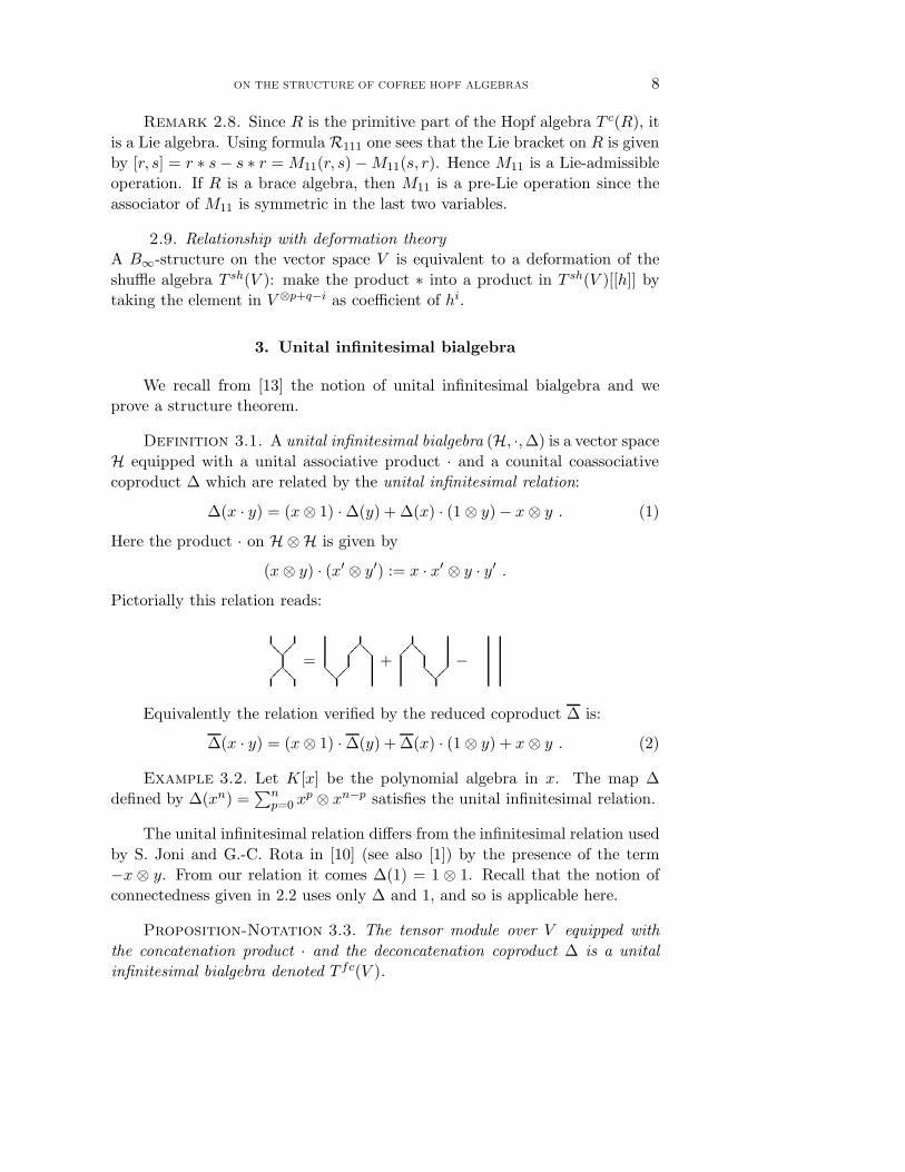
Definition 3.1. A unital infinitesimal bialgebra (H, ·,∆) is a vector space
H equipped with a unital associative product · and a counital coassociative
coproduct ∆ which are related by the unital infinitesimal relation:
∆(x · y) = (x⊗ 1) ·∆(y) + ∆(x) · (1⊗ y)− x⊗ y . (1)
Here the product · on H⊗H is given by
(x⊗ y) · (x′ ⊗ y′) := x · x′ ⊗ y · y′ .
Pictorially this relation reads:
??? ���
��� ???=
��� ???
??? ���+
��� ???
??? ���−
Equivalently the relation verified by the reduced coproduct ∆ is:
∆(x · y) = (x⊗ 1) ·∆(y) + ∆(x) · (1⊗ y) + x⊗ y . (2)
Example 3.2. Let K[x] be the polynomial algebra in x. The map ∆
defined by ∆(xn) =∑n
p=0 xp ⊗ xn−p satisfies the unital infinitesimal relation.
The unital infinitesimal relation differs from the infinitesimal relation used
by S. Joni and G.-C. Rota in [10] (see also [1]) by the presence of the term
−x ⊗ y. From our relation it comes ∆(1) = 1 ⊗ 1. Recall that the notion of
connectedness given in 2.2 uses only ∆ and 1, and so is applicable here.
Proposition-Notation 3.3. The tensor module over V equipped with
the concatenation product · and the deconcatenation coproduct ∆ is a unital
infinitesimal bialgebra denoted T fc(V ).
ON THE STRUCTURE OF COFREE HOPF ALGEBRAS 9
Proof. Let us compute ∆(x · y) for x = u1 . . . up and y = up+1 . . . un :
∆(x · y)=∆(u1 . . . un)
=n∑
i=0
u1 . . . ui ⊗ ui+1 . . . un
=
p∑
i=0
u1 . . . ui ⊗ ui+1 . . . un − u1 . . . up ⊗ up+1 . . . un
+n∑
i=p
u1 . . . ui ⊗ ui+1 . . . un
=∆(u1 . . . up) · (1⊗ up+1 . . . un)− u1 . . . up ⊗ up+1 . . . un
+(u1 . . . up ⊗ 1) ·∆(up+1 . . . un)
=∆(x) · (1⊗ y)− x⊗ y + (x⊗ 1) ·∆(y) .
3.4. Convolution product
For any bialgebra (H, ν,∆) (either classical or unitary infinitesimal) the con-
volution product ⋆ on HomK(H,H) is defined as follows. For f and g ∈
HomK(H,H) one puts
f ⋆ g := ν ◦ (f ⊗ g) ◦∆ .
From the associativity of ν and the coassociativity of ∆ it follows that ⋆ is
associative. It is also easy to check that uc is a unit for ⋆.
Proposition 3.5. Let (H, ν,∆) be a connected unital infinitesimal bial-
gebra. The linear operator e : H → H defined by
e := J − J ⋆ J + · · ·+ (−1)n−1J⋆n + · · ·
where J := Id− uc, has the following properties:
a) Im e = PrimH,
b) for any x, y ∈ H one has e(ν(x, y)) = 0,
c) e is an idempotent,
d) for H = (T (V ), ·,∆), where · is the concatenation and ∆ the decon-
catenation, e is the identity on V and 0 on the other components.
Proof. We adopt the following notation for this proof: ν(x, y) := x · y,
Id = IdH, and, for any x ∈ H,
∆(x) := x(1) ⊗ x(2) . (3)
So we omit the summation symbol in the formula for the reduced comul-
tiplication.
ON THE STRUCTURE OF COFREE HOPF ALGEBRAS 10
First, we observe that, on H, e can be written
e :=∑
r≥0
(−1)rνr ◦∆r= Id− ν ◦∆+ ν2 ◦∆
2+ · · · (4)
and so satisfies the following equality:
e = Id− ν ◦ (Id⊗ e) ◦∆ . (5)
which can be written
e(x) = x− x(1) · e(x(2)) . (6)
a) We proceed by induction on the filtration-degree of x ∈ H. Recall that if
x ∈ FnH, then x(1) and x(2) are in Fn−1H.
If x ∈ F1H = PrimH, then ∆(x) = 0 and therefore e(x) = x by (6). Let
us now suppose that e(y) ∈ PrimH for any y ∈ Fn−1H, and let x ∈ FnH. We
compute
∆(e(x))=∆(x)−∆ ◦ ν ◦ (Id⊗ e) ◦∆(x) by (5)
=x⊗ 1 + 1⊗ x+ x(1) ⊗ x(2) −∆(x(1) · e(x(2))) by (3)
=x⊗ 1 + 1⊗ x+ x(1) ⊗ x(2) −∆(x(1)) · (1⊗ e(x(2)))− x(1) · e(x(2))⊗ 1
by (1) and induction
= e(x)⊗ 1 + 1⊗ x+ x(1) ⊗ x(2) − x(1) ⊗ e(x(2))− 1⊗ x(1) · e(x(2))
−(Id⊗ ν) ◦ (Id⊗ Id⊗ e) ◦∆2(x) by (6)
= e(x)⊗ 1 + 1⊗ e(x) + (Id⊗ (Id− e)) ◦∆(x)− (Id⊗ (Id− e)) ◦∆(x)
by (5)
= e(x)⊗ 1 + 1⊗ e(x) ,
which proves that e(x) is primitive. If x ∈ PrimH, then ∆(x) = 0 and there-
fore e(x) = x by (5).
b) We proceed by induction on the sum of the filtration-degrees of x and y. If
x and y are both primitive, then
∆(x · y) = x⊗ y and ∆r(x · y) = 0 for r ≥ 2.
Therefore we get
e(x · y) = x · y − ν ◦∆(x · y) = x · y − x · y = 0.
We now suppose that the formula holds when the sum of the filtration-degrees
is strictly less than the sum of the filtration-degrees of x and y. We have
e(x · y)=x · y − ν ◦ (Id⊗ e) ◦∆(x · y) by (6)
=x · y − x · y(1) · e(y(2))− x(1) · e(x(2) · y)− x · e(y) by (1) and (3)
=x · y − x · y(1) · e(y(2))− x · e(y) by induction
=x · e(y)− x · e(y) = 0 by (5)
ON THE STRUCTURE OF COFREE HOPF ALGEBRAS 11
and the proof is completed.
(c) Follows immediately from (a), since ∆(x) = 0 when x is primitive.
(d) This assertion is immediate by direct inspection.
Theorem 3.6. Any connected unital infinitesimal bialgebra H is isomor-
phic to T fc(PrimH) := (T (PrimH), ν,∆), where ν = concatenation and ∆ =
deconcatenation.
Proof. Let V := PrimH. Define a bialgebra morphism G : H → T (V ) by
the formula
G(x) :=∑
n≥1
e⊗n ◦∆n−1
(x).
Define F : T (V ) → H by F (v1 . . . vn) := v1 · . . . · vn for n ≥ 1. The composite
F ◦G is equal to∑
n≥1 e⋆n since
F ◦G =∑
n≥1
νn−1 ◦ e⊗n ◦∆n−1
=∑
n≥1
e⋆n.
The two series g(t) := t−t2+t3−. . . = t1+t
and f(t) := t+t2+t3+. . . = t1−t
are
inverse to each other for composition: (f ◦g)(t) = t. We can apply these series
to elements of HomK(H,H) which send 1 to 0 by using ⋆ for multiplication.
We get e = g⋆(J) (cf. Proposition 3.5) and
F ◦G =∑
n≥1
e⋆n = f⋆(e) = f⋆ ◦ g⋆(J) = (f ◦ g)⋆(J) = Id⋆(J) = J.
On the other hand one has
G ◦ F (v1 . . . vn)=G(v1 · . . . · vn)
= e⊗n ◦∆n−1
(v1 · . . . · vn)
= e(v1)⊗ . . .⊗ e(vn)
= v1 ⊗ . . .⊗ vn .
We have used 3.5.b in this computation. We have shown that H and T (V ) are
isomorphic.
Remark 3.7. The idempotent e is the geometric series (for convolution)
applied to the map J = Id − uc. It is the analogue of the first Eulerian
idempotent, which, in the classical case, is defined as the logarithm series
applied to J . The geometric series was already used in a similar context in
[19]. Observe that in our case the characteristic zero hypothesis is not needed
since the geometric series has no denominators.
ON THE STRUCTURE OF COFREE HOPF ALGEBRAS 12
Theorem 3.6 is similar to the Hopf-Borel theorem, cf. [3], which states,
in the non-graded case, that any connected commutative cocommutative Hopf
algebra H is isomorphic to the symmetric algebra S(PrimH) (in characteristic
zero).
4. 2-associative algebra and 2-associative bialgebra
In this section we introduce the algebras with two associative operations,
that we call 2-associative algebras. Then we study the 2-associative algebras
equipped with a cooperation.
Definition 4.1. A 2-associative algebra overK is a vector space A equipped
with two associative operations (x, y) 7→ x∗y and (x, y) 7→ x·y. A 2-associative
algebra is said to be unital if there is an element 1 which is a unit for both
operations. Unless otherwise stated we suppose that the 2-associative algebras
are unital.
Observe that the definition of a 2-associative object makes sense in any
monoidal category. So we can define a notion of 2-associative monoid, of 2-
associative group, of 2-associative monoidal category, of 2-associative operad,
etc.
The free 2-associative algebra over the vector space V is the 2-associative
algebra 2as(V ) such that any map from V to a 2-associative algebra A has a
natural extension as a 2-associative morphism 2as(V ) → A. In other words
the functor 2as(−) is left adjoint to the forgetful functor from 2-associative
algebras to vector spaces. It is clear that 2as(V ) is graded and of the form
2as(V ) = ⊕n≥02asn ⊗ V ⊗n. More information on the explicit structure of
2as(V ), that is on 2asn, is given in section 6.
4.2. Tensor product of 2-associative algebrasGiven two 2-associative algebras A and B we define their tensor product as the
2-associative algebra A⊗B equipped with the two products
(a⊗ b) ∗ (a′ ⊗ b′) := a ∗ a′ ⊗ b ∗ b′,
(a⊗ b) · (a′ ⊗ b′) := a · a′ ⊗ b · b′ .
The unit of A⊗B is 1⊗ 1.
If fi : Ai → A′i (for i = 1, 2) is a morphism of 2-associative algebras, then
obviously f1⊗ f2 : A1⊗A2 → A′1⊗A
′2 is a morphism of 2-associative algebras.
4.3. On 2-associative algebras and B∞-algebras
Let (A, ∗, ·) be a 2-associative algebra. We define (p+ q)-ary operations Mpq :
A⊗p+q → A, for p ≥ 0, q ≥ 0 by induction as follows:
M00 = 0, M10 = IdA =M01, and Mn0 = 0 =M0n for n ≥ 2,
ON THE STRUCTURE OF COFREE HOPF ALGEBRAS 13
and
Mpq(u1 . . . up, v1 . . . vq) :=(u1 · u2 · . . . · up
)∗(v1 · v2 · . . . · vq
)
−∑
k≥2
∑
(i,j)
(Mi1j1 · . . . ·Mikjk(u1 . . . up, v1 . . . vq)
)(1)
where the second sum (for which k ≥ 2 is fixed) is extended to all the sets of
indices (i, j) such that i1 + · · · + ik = p and j1 + · · ·+ jk = q.
For instance (cf. 2.4):
M11(u, v)=u ∗ v − u · v − v · u ,
M21(uv,w) = (u · v) ∗ w − u ·M11(v,w) −M11(u,w) · v
−u · v · w − u · w · v − w · u · v
=(u · v) ∗ w − u · (v ∗ w) − (u ∗ w) · v + u · w · v ,
M12(u, vw) =u ∗ (v · w)−M11(u, v) · w − v ·M11(u,w)
−u · v · w − v · u · w − v · w · u
=u ∗ (v · w)− (u ∗ v) · w − v · (u ∗ w) + v · u · w .
Proposition 4.4. The family of (p + q)-ary operations Mpq constructed
above defines a functor
(−)B∞: {2as−algebras} −→ {B∞−algebras}.
Proof. Let us write Idi for Id⊗i. We want to prove that, for any integers
p, q, r ≥ 1, the following formula (denoted Rpqr in 2.4) holds:
∑
(p,q)
Mlr ◦ (Mp1q1 · · ·Mplql ⊗ Idr) =∑
(q,r)
Mps ◦ (Idp ⊗Mq1r1 · · ·Mqsrs),
where the left sum is taken over all the partitions
(p, q) = (p1, · · · , pl; q1, · · · , ql)
with 1 ≤ l ≤ p + q, 0 ≤ pi ≤ p, 0 ≤ qi ≤ q,∑
i pi = p and∑
i qi = q, and
the right sum is taken over all partitions (q, r) = (q1, · · · , qs; r1, · · · , rs) with
1 ≤ s ≤ q + r, 0 ≤ qj ≤ q, 0 ≤ rj ≤ r,∑
j qj = q and∑
j rj = r.
We use the following notation: µ(x, y) := x ∗ y, ν(x, y) := x · y,
νn−1(u1 . . . un) := u1 · . . . · un and νp,q,r := νp−1 ⊗ νq−1 ⊗ νr−1 .
We will prove, by induction on h = p + q + r that the difference of the two
sums is equal to
µ ◦ (µ⊗ Idr) ◦ (νp,q,r)− µ ◦ (Idp ⊗ µ) ◦ (νp,q,r)
ON THE STRUCTURE OF COFREE HOPF ALGEBRAS 14
and so is 0 by the associativity property of µ.
Let us first check the property for p = q = r = 1, i.e. h = 3. Consider the
two sums
Sl :=M21(uv + vu,w) +M11(M11(u, v), w),
Sr :=M12(u, vw + wv) +M11(u,M11(v,w)) .
By replacing the elements by their value in terms of the operations ∗ and ·
we get, up to a permutation of variables, the following 8 different types of
elements: (− ◦1 −) ◦2 − and − ◦1 (− ◦2 −) for ◦i = ∗ or · . Collecting the
terms of type (− · −) · − (resp. − ∗ (− · −) ) in Sl gives 0 and similarly in Sr.
Collecting the terms of type (− ∗ −) · − (resp. − · (− ∗ −), resp. − · (− ∗ −),
resp. −· (−·−) ) in Sl gives the same element as in Sr. Collecting the terms of
type (−∗−) ∗− or −∗ (−∗−) in Sl gives (u ∗ v) ∗w and in Sr gives u ∗ (v ∗w).
Hence by the associativity property of ∗ we get Sl = Sr, i.e. relation R111.
For h ≥ 4, observe that the following equalities hold:
µ ◦ (µ ⊗ Idr) ◦ νp,q,r =
∑
(p,q)
Mlr ◦ (Mp1q1 · · ·Mplql ⊗ Idr)+
ν◦( ∑
k+m+n<h
µ◦(µ⊗Idr−m)◦νp−k,q−m,r−n ⊗∑
(k,m)
Mlm◦(Mk1n1· · ·Mklnl
⊗Idm)),
and
µ ◦ (Idp ⊗ µ) ◦ (νp,q,r) =∑
(q,r)
Mps ◦ (Idp ⊗Mq1r1 · · ·Mqsrs)+
ν◦( ∑
k+m+n<h
µ◦(Idp−k⊗µ)◦νp−k,q−m,r−n⊗
∑
(n,m)
Mks◦(Idk⊗Mn1m1· · ·Mnsqm)
).
The recursion hypothesis and the associativity of µ imply that
ν◦( ∑
k+m+n<h
µ◦(µ⊗Idr−m)◦νp−k,q−m,r−n ⊗∑
(k,m)
Mlm◦(Mk1n1· · ·Mklnl
⊗Idm))
= ν◦( ∑
k+m+n<h
µ◦(Idp−k⊗µ)◦νp−k,q−m,r−n⊗
∑
(n,m)
Mks◦(Idk⊗Mn1m1· · ·Mnsqm)
).
So, taking the difference, we get∑
(p,q)
Mlr ◦ (Mp1q1 · · ·Mplql ⊗ Idr)−∑
(q,r)
Mps ◦ (Idp ⊗Mq1r1 · · ·Mqsrs)
= µ ◦ (µ⊗ Idr) ◦ (νp,q,r)− µ ◦ (Idp ⊗ µ) ◦ (νp,q,r),
as expected.
Corollary 4.5. Let R be a B∞-algebra and let (T c(R), ∗,∆) be the as-
sociated bialgebra. Put on T c(R) the B∞-algebra structure induced by the 2-
associative operations ∗ and · (concatenation). Then the inclusion R→ T c(R)
ON THE STRUCTURE OF COFREE HOPF ALGEBRAS 15
is a B∞-morphism. In other words the B∞-algebra structure of R has been
extended to T c(R).
Proof. The operation ∗ is given by Proposition 2.6 and the operation · is
concatenation. Denote by Mpq the B∞-structure on R and by Mpq the B∞-
structure on T c(R) given by Proposition 4.4. Let us show that Mpq =Mpq on
R⊗p+q by induction on p + q. We use formula (1) which holds for M and M
on R. By induction M = M on the right side, therefore Mpq = Mpq for any
(p, q).
4.6. Universal enveloping 2-associative algebra
We define the universal enveloping 2-associative algebra of a B∞-algebra R,
denoted U2(R), as the quotient of the free 2-associative algebra 2as(R) over
the vector space R by the relations
Mpq(r1 · · · rp, s1 · · · sq) ≈ Mpq(r1 · · · rp, s1 · · · sq), ri, sj ∈ R
where Mpq denotes the operation in R and Mpq denotes the operation in
2as(R):
U2(R) := 2as(R)/ ≈ .
In other words we divide 2as(R) by the ideal (in the 2-associative algebra
sense) generated by the elements
Mpq(r1 · · · rp, s1 · · · sq)− Mpq(r1 · · · rp, s1 · · · sq),
thus U2(R) is a 2-associative algebra.
Lemma 4.7. The functor U2 : {B∞−alg} −→ {2as−alg} is left adjoint
to the functor (−)B∞: {2as−alg} −→ {B∞ −alg} .
Proof. Let A be a 2as-algebra and let f : R → AB∞be a morphism
of B∞-algebras. It determines uniquely a morphism of 2-associative algebras
2as(R) → A since A is a 2-associative algebra and 2as(R) is free. This mor-
phism passes to the quotient to give U2(R) → A because the image in A of
the two elements
Mpq(r1 · · · rp, s1 · · · sq) and Mpq(r1 · · · rp, s1 · · · sq),
is the same, namely Mpq(f(r1) · · · f(rp), f(s1) · · · f(sq)).
On the other hand, let g : U2(R) → A be a morphism of 2-associative
algebras. From the construction of U2(R) it follows that the map R→ U2(R)
is a B∞-morphism. Hence the composition with g gives a B∞-morphism R→
A.
Clearly these two constructions are inverse to each other, and therefore
U2 is left adjoint to (−)B∞.
ON THE STRUCTURE OF COFREE HOPF ALGEBRAS 16
Corollary 4.8. The universal enveloping 2-associative algebra of the
free B∞-algebra is canonically isomorphic to the free 2-associative algebra:
U2(B∞(V )) ∼= 2as(V ) .
Proof. First recall that AB∞has the same underlying vector space as A.
Since U2 is left adjoint to (−)B∞and since B∞ is left adjoint to the forgetful
functor, the composite is left adjoint to the forgetful functor from 2-associative
algebras to vector spaces. Hence it is the functor 2as.
Definition 4.9. A 2-associative bialgebra (resp. 2-associative Hopf alge-
bra) (H, ∗, ·,∆) is a vector space H equipped with two operations ∗ and · and
one cooperation ∆, such that
• (H, ∗,∆) is a bialgebra (resp. Hopf algebra), cf. 2.1,
• (H, ·,∆) is a unital infinitesimal bialgebra, cf. 3.1.
Proposition 4.10. For any 2-associative bialgebra (e.g. 2-associative
Hopf algebra) its primitive part is a sub-B∞-algebra.
Proof. Given elements x1, . . . , xn, y1, . . . , ym in PrimH, we need to prove
that Mnm(x1 . . . xn, y1 . . . ym) belongs to PrimH too, that is ∆ ◦Mnm = 0 on
PrimH. The proof is by induction on (n,m). Instead of giving the details we
give an alternate proof in the case where H is connected. We only need this
case in the sequel of the article.
IfH is a connected 2-associative bialgebra, thenH is isomorphic to T fc(PrimH)
by Theorem 3.6 and PrimH is a B∞-algebra. So we can apply Corollary 4.5.
Proposition 4.11. There exists a unique cooperation ∆ on the free 2-
associative algebra 2as(V ) which makes it into a 2-associative bialgebra and
for which V is primitive. As a coalgebra 2as(V ) is connected.
Proof. We define ∆ : 2as(V ) → 2as(V )⊗2as(V ) by the following require-
ments:
• ∆(1) = 1⊗ 1,
• ∆(v) = v ⊗ 1 + 1⊗ v, for v ∈ V ,
• ∆(x ∗ y) = ∆(x) ∗∆(y),
• ∆(x · y) = (x⊗ 1) ·∆(y) + ∆(x) · (1⊗ y)− x⊗ y.
Let us prove that ∆ is well-defined by induction on the degree of the
elements in 2as(V ) = ⊕n≥02as(V )n. It is already defined on 2as(V )0 = K.1
and 2as(V )1 = V . Suppose that ∆ is defined up to 2as(V )n−1. We define it
on 2as(V )n as follows. Any element of 2as(V )n is of the form x ∗ y or x · y
ON THE STRUCTURE OF COFREE HOPF ALGEBRAS 17
for elements x and y of degree strictly smaller than n. Then ∆(x ∗ y) and
∆(x · y) are given by the required formulas. Since the only relations are the
associativity of ∗, the associativity of · and the unitality of 1 for both products,
we need to verify that
∆((x ∗ y) ∗ z) = ∆(x ∗ (y ∗ z)),
∆((x · y) · z) = ∆(x · (y · z)),
∆(1 ∗ x) = ∆(x) = ∆(x ∗ 1),
∆(1 · x) = ∆(x) = ∆(x · 1).
The last two lines are straightforward to check. The first one is classical. Let
us check the second one. On the left side we get (with the notation a ·∆(b) =
(a⊗ 1) ·∆(b) and ∆(a) · b = ∆(a) · (1⊗ b) )
∆((x · y) · z)= (x · y) ·∆(z) + ∆(x · y) · z − (x · y)⊗ z,
=x · y ·∆(z) + (x ·∆(y) + ∆(x) · y − x⊗ y) · z − x · y ⊗ z,
=x · y ·∆(z) + x ·∆(y) · z +∆(x) · y · z − x⊗ y · z − x · y ⊗ z .
On the right side we get
∆(x · (y · z))=x ·∆(y · z) + ∆(x) · (y · z)− x⊗ y · z,
=x · (y ·∆(z) + ∆(y) · z − y ⊗ z) + ∆(x) · y · z − x⊗ y · z,
=x · y ·∆(z) + x ·∆(y) · z +∆(x) · y · z − x⊗ y · z − x · y ⊗ z .
We see that they are equal. Hence ∆ is well-defined. There is a unique map
2as(V ) → 2as(V ) ⊗ 2as(V ) ⊗ 2as(V ) sending 1 to 1 ⊗ 1 ⊗ 1 and v to v ⊗
1 ⊗ 1 + 1 ⊗ v ⊗ 1 + 1 ⊗ 1 ⊗ v and compatible with ∗ and ·. Since both maps
(∆⊗ Id) ◦∆ and (Id⊗∆) ◦∆ satisfy these properties, they are equal, and so
∆ is coassociative.
It follows from this computation that (2as(V ), ∗, ·,∆) is a 2-associative
bialgebra.
Proof of connectedness. It is sufficient to prove that any element in H is
conilpotent. An element in 2as(V )/K is primitive, hence conilpotent. So it
suffices to prove that, if x and y are conilpotent, then so are x ∗ y and x · y.
This fact follows from the relationship between ∆ and ∗, respectively ∆ and ·.
Corollary 4.12. For any B∞-algebra R, U2(R) is a connected 2-asso-
ciative bialgebra. �
5. The main theorem
In this section we state and prove the main results, that is the structure
theorem for cofree Hopf algebras and the main theorem from which it follows,
ON THE STRUCTURE OF COFREE HOPF ALGEBRAS 18
that is the structure theorem for connected 2-associative bialgebras. They
are analogue of the Cartier-Milnor-Moore theorem (for (a)⇒ (b)) and the
Poincare-Birkhoff-Witt theorem (for (b)⇒ (c)), which hold for cocommutative
connected bialgebras (over a characteristic zero field). Observe that in the
non-cocommutative setting we do not need the characteristic zero hypothesis.
5.1. Classification of cofree bialgebrasA connected cofree bialgebra can be equipped with a second product (by using
cofreeness) which makes it into a connected 2-associative bialgebra. Our main
result about these objects is the following.
Theorem 5.2. If H is a bialgebra over a field K, then the following are
equivalent:
(a) H is a connected 2-associative bialgebra,
(b) H is isomorphic to U2(PrimH) as a 2-associative bialgebra,
(c) H is cofree among the connected coalgebras.
Since a connected bialgebra is a Hopf algebra, one can replace connected
bialgebra by connected Hopf algebra in this theorem.
Proof. We prove the following implications (a) ⇒ (c) ⇒ (b) ⇒ (a). We
put R := PrimH.
(a) ⇒ (c). If H is a connected 2-associative bialgebra, then, by Theorem 3.6,
H is isomorphic to T fc(R) as a unital infinitesimal bialgebra. Therefore H is
cofree.
(c) ⇒ (b). If H is cofree, then it is isomorphic to T fc(R) and R is a B∞-
algebra. Observe that T fc(R) is a 2as-algebra: the product ∗ is inherated
from the associative product of H under the isomorphism and the product
· is the concatenation. By adjunction (cf. Lemma 4.7), the inclusion map
R→ T fc(R) gives rise to a 2as-morphism
φ : U2(R) → T fc(R) .
On the other hand, the inclusion R→ U2(R) admits a unique extension
ψ : T fc(R) → U2(R)
by ψ(r1 . . . rn) = ψ(r1) · . . . · ψ(rn). It is immediate to check that φ and ψ are
inverse to each other.
(b) ⇒ (a). This is Corollary 4.12.
As an immediate consequence, we obtain a structure theorem for cofree
bialgebras:
Corollary 5.3. There is an equivalence between the category of cofree
bialgebras and the category of bialgebras of the form U2(R) for some B∞-
algebra R.
ON THE STRUCTURE OF COFREE HOPF ALGEBRAS 19
�
The particular case of free algebras reads as follows:
Corollary 5.4. For any vector space V the free 2-associative algebra
2as(V ) and the free B∞-algebra B∞(V ) are related by the following isomor-
phisms:
φ : Prim (2as(V )) ∼= B∞(V ) as B∞-algebras,
φ : 2as(V ) ∼= T fc(B∞(V )) as 2-associative bialgebras.
�
5.5. The differential graded framework
So far we worked in the category of vector spaces over K. However we can,
more generally, work in the category of graded vector spaces, or differential
graded vector spaces (that is chain complexes), in which all the constructions
and results remain true. In the graded case the formulas are exactly the same
as in the non-graded case, provided we write them as equalities among maps,
that is we forget the entries. For instance the relation (R111) should be written:
M21 ◦ ((12) + 13) +M11 ◦ (M11 ⊗ 11) =M12 ◦ (13 + (23)) +M11 ◦ (11 ⊗M11) .
In this formula 13 is the identity on V ⊗3 and (12) is the map which permutes
the first two variables, so
(12)(uvw) = (−1)|u||v|vuw
where |u| is the degree of the homogeneous element u. One should also use
the Koszul sign rule, that is f ⊗ g means the map which sends u ⊗ v to
(−1)|g||u|f(u)⊗ g(v).
In the differential graded case, a B∞-algebra structure on the graded vec-
tor space V = ⊕n∈ZV⊗n is equivalent to a graded differential algebra structure
on the tensor coalgebra T (V [1]) where V [1] is the desuspension of V (cf. [7]
or [21] for details).
5.6. The dual framework
Instead of starting with a bialgebra which is cofree as a coalgebra, we
could start with a bialgebra which is free as an algebra. Then similar results
hold, but 2-associative algebras have to be replaced by 2-coassociative coalge-
bras and so forth. Observe that the notion of unital infinitesimal bialgebra is
self-dual (this is easily seen on the picture of 3.1). See 7.4 for the free case.
ON THE STRUCTURE OF COFREE HOPF ALGEBRAS 20
6. Free 2-associative algebra
In this section we give an explicit description of the free 2-associative
algebra in terms of planar trees. The free 2as-algebra on one generator can
be identified with the non-commutative polynomials over the planar (rooted)
trees. Alternatively the underlying vector space can be identified with the
vector space spanned by two copies of the set of planar trees amalgamated
over the trivial tree.
We study the operad associated to 2-associative algebras, we compute its
dual (in the operadic sense) and we show that they are Koszul operads. As
a consequence we obtain a chain complex to compute the (co)homology of
2-associative algebras.
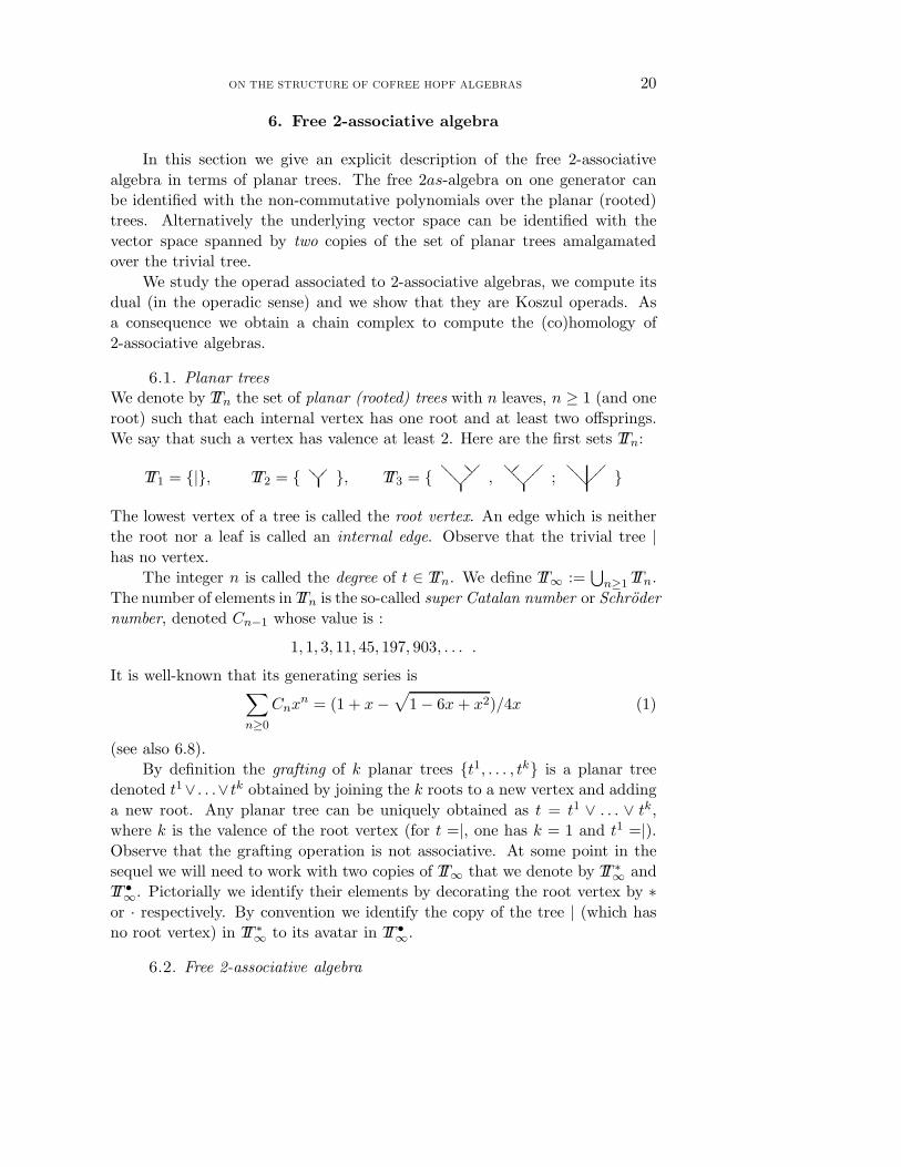
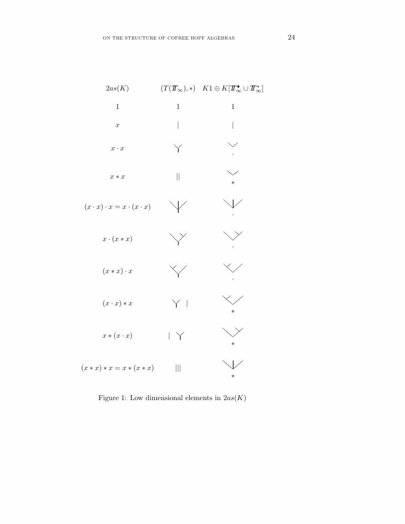
6.1. Planar treesWe denote by TTn the set of planar (rooted) trees with n leaves, n ≥ 1 (and one
root) such that each internal vertex has one root and at least two offsprings.
We say that such a vertex has valence at least 2. Here are the first sets TTn:
TT1 = {|}, TT2 = { ��??
}, TT3 = {??����
???? ,�� ����
???? ;����
???? }
The lowest vertex of a tree is called the root vertex. An edge which is neither
the root nor a leaf is called an internal edge. Observe that the trivial tree |
has no vertex.
The integer n is called the degree of t ∈ TTn. We define TT∞ :=⋃
n≥1 TTn.
The number of elements in TTn is the so-called super Catalan number or Schroder
number, denoted Cn−1 whose value is :
1, 1, 3, 11, 45, 197, 903, . . . .
It is well-known that its generating series is∑
n≥0
Cnxn = (1 + x−
√1− 6x+ x2)/4x (1)
(see also 6.8).
By definition the grafting of k planar trees {t1, . . . , tk} is a planar tree
denoted t1∨ . . .∨ tk obtained by joining the k roots to a new vertex and adding
a new root. Any planar tree can be uniquely obtained as t = t1 ∨ . . . ∨ tk,
where k is the valence of the root vertex (for t =|, one has k = 1 and t1 =|).
Observe that the grafting operation is not associative. At some point in the
sequel we will need to work with two copies of TT∞ that we denote by TT ∗∞ and
TT •∞. Pictorially we identify their elements by decorating the root vertex by ∗
or · respectively. By convention we identify the copy of the tree | (which has
no root vertex) in TT ∗∞ to its avatar in TT •
∞.
6.2. Free 2-associative algebra
ON THE STRUCTURE OF COFREE HOPF ALGEBRAS 21
Since, in the relations defining the notion of 2-associative algebra, the variables
stay in the same order, we only need to understand the free 2-associative
algebra on one generator (i.e. over K). In operadic terminology we are dealing
with a regular operad (i.e. constructed out of a non-Σ-operad).
More explicitly, if we denote by 2as(K) = ⊕n≥02asn the free 2-associative
algebra on one generator, then the free 2-associative algebra on V is
2as(V ) =⊕
n≥0
2asn ⊗ V ⊗n .
The 2-associative structure of 2as(V ) is induced by the 2-associative structure
of 2as(K) and concatenation of tensors:
(s; v1 · · · vp) ∗ (t, vp+1 · · · vn)= (s ∗ t; v1 · · · vn),
(s; v1 · · · vp) · (t, vp+1 · · · vn)= (s · t; v1 · · · vn).
Let T (TT∞) = (T (K[TT∞]), ∗) be the free unital associative algebra over the
vector spaceK[TT∞] generated by the set TT∞. So here ∗ is the concatenation. A
set of linear generators of T (TT∞) is made of the (non-commutative) monomials
t1∗t2∗· · ·∗tk where the ti’s are planar trees. We define the product · as follows:
s · t := s1 ∨ . . . ∨ sm ∨ t1 ∨ . . . ∨ tn,
(s1 ∗ . . . ∗ sk) · t := (s1 ∨ . . . ∨ sk) ∨ t1 ∨ . . . ∨ tn, for k ≥ 2,
s · (t1 ∗ . . . ∗ tl) := s1 ∨ . . . ∨ sm ∨ (t1 ∨ . . . ∨ tl), for l ≥ 2,
(s1 ∗ . . . ∗ sk) · (t1 ∗ . . . ∗ tl) := (s1 ∨ . . . ∨ sk) ∨ (t1 ∨ . . . ∨ tl), for k ≥ 2, l ≥ 2,
where s = s1 ∨ . . . ∨ sm and t = t1 ∨ . . . ∨ tn.
Observe that the dot product of two monomials is always a tree.
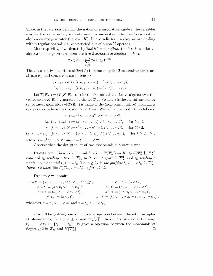
Lemma 6.3. There is a natural bijection T (TT∞) → K1 ⊕ K[TT ∗∞
⋃TT •
∞]
obtained by sending a tree in TT∞ to its counterpart in TT •∞ and by sending a
nontrivial monomial t1 ∗ · · · ∗ tn (i.e. n ≥ 2) to the grafting t1∨ . . .∨ tn in TT ∗∞.
Hence we have dimT (TT∞)n = 2Cn−1 for n ≥ 2.
Explicitly we obtain:
s∗ ∗ t∗ = (s1 ∨ . . . ∨ sn ∨ t1 ∨ . . . ∨ tm)∗, s∗ · t∗ = (s ∨ t)·,
s· ∗ t∗ = (s ∨ t1 ∨ . . . ∨ tm)∗, s· · t∗ = (s1 ∨ . . . ∨ sn ∨ t)·,
s∗ ∗ t· = (s1 ∨ . . . ∨ sn ∨ t)∗, s∗ · t· = (s ∨ t1 ∨ . . . ∨ tm)·,
s· ∗ t· = (s ∨ t)∗, s· · t· = (s1 ∨ . . . ∨ sn ∨ t1 ∨ . . . ∨ tm)·,
whenever s = s1 ∨ . . . ∨ sn and t = t1 ∨ . . . ∨ tm.
Proof. The grafting operation gives a bijection between the set of n-tuples
of planar trees, for any n ≥ 2, and TT∞\{|}. Indeed the inverse is the map
t1 ∨ · · · ∨ tn 7→ {t1, · · · , tn}. It gives a bijection between the monomials of
degree ≥ 2 in TT∞ and K[TT •∞].
ON THE STRUCTURE OF COFREE HOPF ALGEBRAS 22
Theorem 6.4. The free 2-associative algebra 2as(K) on one generator is
isomorphic to the 2-associative algebra (T (TT∞), ∗, ·) where ∗ is the concatena-
tion product in T (TT∞) and · is given by the formulas in 6.2.
Proof. First we check that the dot product is associative. There are eight
cases, which are immediate to check. For instance, if u = u1 ∨ . . . ∨ up, then
(s · t) · u = s1 ∨ . . . ∨ sm ∨ t1 ∨ . . . ∨ tn ∨ u1 ∨ . . . ∨ up = s · (t · u) .
Second we prove that, as a 2as-algebra, it is free on one generator. Let x
be the generator of the free 2-associative algebra 2as(K) = ⊕n≥02asn. Since
T (TT∞) is a 2-associative algebra, mapping x to the tree | induces a 2-associative
morphism α : 2as(K) → T (TT∞). Since any linear generator of T (TT∞) can be
obtained from | by using ∗ and ·, this map is surjective. The degree n part
of T (TT∞) is of dimension 2Cn−1 by Lemma 6.3, hence to prove that α is an
isomorphism it suffices to prove that the dimension of 2asn is less than or equal
to 2Cn−1.
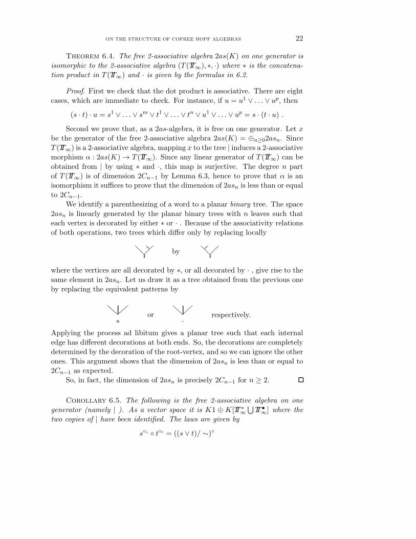
We identify a parenthesizing of a word to a planar binary tree. The space
2asn is linearly generated by the planar binary trees with n leaves such that
each vertex is decorated by either ∗ or · . Because of the associativity relations
of both operations, two trees which differ only by replacing locally
??����
???? by�� ����
????
where the vertices are all decorated by ∗, or all decorated by · , give rise to the
same element in 2asn. Let us draw it as a tree obtained from the previous one
by replacing the equivalent patterns by
zzzzz
DDDDD
∗or
||||
BBBB
·respectively.
Applying the process ad libitum gives a planar tree such that each internal
edge has different decorations at both ends. So, the decorations are completely
determined by the decoration of the root-vertex, and so we can ignore the other
ones. This argument shows that the dimension of 2asn is less than or equal to
2Cn−1 as expected.
So, in fact, the dimension of 2asn is precisely 2Cn−1 for n ≥ 2.
Corollary 6.5. The following is the free 2-associative algebra on one
generator (namely | ). As a vector space it is K1 ⊕ K[TT ∗∞
⋃TT •
∞] where the
two copies of | have been identified. The laws are given by
s◦s ◦ t◦t = ((s ∨ t)/ ∼)◦
ON THE STRUCTURE OF COFREE HOPF ALGEBRAS 23
where ◦s, ◦t and ◦ are either ∗ or ·, and the quotient ∼ is as follows: the edge
from the root of s (resp. t) to the new root is collapsed to a point if ◦s = ◦
(resp. ◦t = ◦).
�
Remark 6.6. One can switch the roles of the two products, in particular
2as(V ) is free as an associative algebra for · .
A free 2-associative set is called a duplex in [17]. Corollary 6.5 gives also
the structure of the free duplex in one generator.
Observe that for s = s1 ∨ . . . ∨ sn one has
s∗ = s·1 ∗ . . . ∗ s·n and s· = s∗1 · . . . · s
∗n .
In figure 1 we draw the elements in low dimension.
6.7. Involution
Let us define a map ι : 2as(V ) → 2as(V ) by the following requirements:
ι(1) = 1, ι(v) = v, ι(x ∗ y) = ι(y) ∗ ι(x), ι(x · y) = ι(y) · ι(x).
First, it is immediate to verify that ι2 = Id. Second, by using the compatibility
relations between ∆ and the products one can show that
∆(ι(x)) = ι(x(2))⊗ ι(x(1)),where ∆(x) = x(1) ⊗ x(2).
On the trees this involution is simply the symmetry around the root axis.
6.8. Generating series
Let C(x) :=∑
n≥0 Cnxn be the generating series for the super Catalan num-
bers. For a graded vector space V = ⊕n≥0Vn we denote by
fV (x) :=∑
n≥0
dimVn xn
its generating series. Therefore the generating series of K[TT∞] is fK[TT∞](x) =
xC(x), while the generating series of 2as(K) is f2as(x) = 1 − x + 2xC(x).
Since 2as(K) = T (K[TT∞]) one has f2as(x) = (1 − fK[TT∞](x))−1. It follows
that C(x) satisfies the algebraic relation 2xC(x)2 − (1 + x)C(x) + 1 = 0. We
deduce from it the expression given in 6.1:∑
n≥0
Cnxn = (1 + x−
√1− 6x+ x2)/4x .
6.9. Homology and Koszul duality
In [8] Ginzburg and Kapranov developed the theory of Koszul duality for binary
quadratic operads. When an operad is Koszul, its Koszul dual permits us to
construct a small chain complex to compute the homology of algebras and
ON THE STRUCTURE OF COFREE HOPF ALGEBRAS 24
2as(K) (T (TT∞), ∗) K1⊕K[TT •∞ ∪ TT ∗
∞]
1 1 1
x | |
x · x ��?? zz
DD
·
x ∗ x ||xxx
FFF
∗
(x · x) · x = x · (x · x)����
????||||
BBBB
·
x · (x ∗ x)??����
????
DD||||
BBBB
·
(x ∗ x) · x�� ����
????zz ||||
BBBB
·
(x · x) ∗ x ��??
|ww zzzzz
DDDDD
∗
x ∗ (x · x) | ��??
GGzzzzz
DDDDD
∗
(x ∗ x) ∗ x = x ∗ (x ∗ x) |||zzzzz
DDDDD
∗
Figure 1: Low dimensional elements in 2as(K)
ON THE STRUCTURE OF COFREE HOPF ALGEBRAS 25
also to construct the minimal model, hence giving rise to the algebras up to
homotopy. This theory is applicable here and we describe the outcome.
Until the end of this section we work in the nonunital framework, that is
we do not suppose that the 2-associative algebras have a unit. In particular
the degree zero component of the free 2-associative algebra is 0. Let us recall
that the Hochschild chain complex of a nonunital associative algebra A is of
the form
· · · → A⊗n b′−→A⊗n−1 → · · · → A
where b′ is given by b′(a1, · · · , an) =∑i=n−1
i=1 (−1)i(a1, · · · , aiai−1, · · · , an). Its
homology is denoted HAs∗ (A).
From the definition of the dual of an operad (cf. loc.cit. or [12] Appendix
B, for a brief introduction), the dual of the operad 2as is the operad 2as! whose
algebras have two associative operations ∗ and · verifying:
(x ∗ y) · z= 0 =x ∗ (y · z)
(x · y) ∗ z= 0 =x · (y ∗ z)
It is clear that the free 2as!-algebra over V is V in dimension 1 and the sum
of two copies of V ⊗n in dimension n ≥ 2, the first one corresponding to ∗ and
the second one to · . Hence the chain complex of a 2-associative algebra is two
copies of the Hochschild complex described above, amalgamated in dimension
1. To check the Koszulity of the operad 2as it suffices to show that the chain
complex of the free 2as-algebra is acyclic. Since 2as(V ) is free as an associative
algebra for ∗ by Theorem 6.4, and also free as an associative algebra for ·
(cf. 6.6), the corresponding Hochschild complexes are acyclic and hence we
have proved the following:
Proposition 6.10. The operad of 2-associative algebras is a Koszul op-
erad.
�
As a consequence, for a 2as-algebra (A, ∗, ·) we have, for n ≥ 3,
H2asn (A) = HAs
n (A, ∗) ⊕HAsn (A, ·) .
7. Bialgebra structure of the free 2as-algebra and free B∞-algebra
We unravel the Hopf algebra structure of the free 2-associative algebra.
From Theorem 5.2 and the explicitation of the free 2-associative algebra we
deduce the structure of the operad B∞.
7.1. The coproduct on 2as(V )
Proposition 4.11 determines a unique coproduct ∆ on 2as(V ), for which
(2as(V ), ∗,∆) is a Hopf algebra. The following Proposition gives a recursive
ON THE STRUCTURE OF COFREE HOPF ALGEBRAS 26
formula for ∆ in terms of V -decorated trees. By definition a V -decorated tree
is an element (t; v1 . . . vn) ∈ TT n× V ⊗n. It is helpful to think of the entry vi as
a decoration of the ith leaf of the tree t.
Proposition 7.2. The coproduct ∆ on the free 2-associative algebra T (TT∞)
is given recursively by the following formula
∆(t1 ∨ . . . ∨ tr) = 1⊗ t+
r∑
i=1
∨(t1, . . . , ti−1) · ti{1} ⊗ ti{2} ·
∨(ti+1, . . . , tr),
where
∨(t1, . . . , tk) :=
{t1 ∨ . . . ∨ tk if k > 1,
t1(1) . . . t1(n) if k = 1 and t1 = t1(1) ∨ . . . ∨ t1(n),
and we use the notation s{1} ⊗ s{2} := ∆(s1 · · · sk) − 1 ⊗ s1 · · · sk for s =
s1 ∨ · · · ∨ sk, and the convention 1 ∨ ω = ω.
Proof. It is straightforward (though tedious) to check by induction that
this map ∆ satisfies the four identities explicitly written at the beginning of
the proof of Proposition 4.11. For instance we have
∆(|; v) = 1⊗ (|; v) + (|; v) ⊗ 1.
Examples 7.3.
∆( ��??
;uv) = (|;u)⊗ (|; v),
∆(�� ����
???? ;uvw) = (|;u)(|; v) ⊗ (|;w) + (|;u)⊗ ( ��??
; vw) + (|; v) ⊗ ( ��??
;uw),
∆(�� ����
������
?????? ;uvwx) = ( ��??
;uv)(|;w) ⊗ (|;x) + ( ��??
;uv) ⊗ ( ��??
;wx)
+(|;w)⊗ (����
???? ;uvx) + (|;u) ⊗ (�� ����
???? ; vwx) + (|;u)(|, w) ⊗ ( ��??
; vx).
7.4. Selfduality of 2as(V )
On the 2-associative bialgebra (2as(V ), ∗, ·,∆) one can construct another coas-
sociative cooperation δ by the following requirements:
• δ(1) = 1⊗ 1,
• δ(v) = v ⊗ 1 + 1⊗ v, for v ∈ V ,
• δ(x ∗ y) = (x⊗ 1) ∗ δ(y) + δ(x) ∗ (1⊗ y)− x⊗ y,
• δ(x · y) = δ(x) · δ(y).
ON THE STRUCTURE OF COFREE HOPF ALGEBRAS 27
In other words, the compatibility relation between the products ∗, · and
the coproducts ∆, δ is either the classical one (cl) or the unitary infinitesimal
one (ui):
∗ ·
∆ cl ui
δ ui cl
Hence, (2as(V ), ∗, ·,∆, δ) is, at the same time, a free 2-associative algebra
and a cofree 2-associative coalgebra.
Observe that (2as(V ), ·, ∗, δ) is also a free 2-associative bialgebra. In fact
the identity on V induces an isomorphism
(2as(V ), ∗, ·,∆, δ) ∼= (2as(V ), ·, ∗, δ,∆).
7.5. The operad B∞
To unravel the structure of the operad B∞, that is to describe explicitly the
free B∞-algebra B∞(V ), we will use the idempotent e : 2as(V ) → 2as(V )
constructed in Proposition 3.5. Recall that, a priori, B∞(V ) = B∞(n)⊗SnV ⊗n
, where the right Sn-module B∞(n) is the space of n-ary operations. By
Corollary 6.5 2as(V ) admits the following decomposition:
2as(V ) = K1⊕ V ⊕⊕
n≥2
K[TT ∗n ]⊗ V ⊗n ⊕
⊕
n≥2
K[TT •n ]⊗ V ⊗n.
We denote by t∗, resp. t•, the image of the decorated tree t ∈ K[TTn]⊗V ⊗n in
the relevant component of 2as(V ). Under this identification, the idempotent
e has the following properties:
e(1) = 0, e(v) = v, e(t∗) = t∗ + ω(t)• , e(t•) = 0,
where t ∈ K[TTn] ⊗ V ⊗n, n ≥ 2, is a decorated tree and where ω : K[TTn] ⊗
V ⊗n → K[TTn]⊗ V ⊗n is a functorial map in V determined by e.
Let us denote by γp,q ∈ TTp+q the tree which is the grafting of the p-corolla
with the q-corolla. So γpq has p+ q leaves and 3 vertices:
??��??��
γ32 =HHHH
vvvv
Theorem 7.6. The free B∞-algebra over the vector space V is
B∞(V ) ∼=⊕
n≥1
K[TTn]⊗ V ⊗n,
where TTn is the set of planar rooted trees. Under this isomorphism the opera-
tion Mpq ∈ B∞(p + q) corresponds to (γpq ⊗ 1p+q) ∈ K[TTp+q]⊗K[Sp+q]. The
ON THE STRUCTURE OF COFREE HOPF ALGEBRAS 28
composition of operations in B∞(V ) is determined by the following equality
which holds in 2as(V ) (in fact in the ∗-component):
Mpq(t1 . . . tp, tp+1 . . . tp+q)∗ =
(e(t∗1) · . . . · e(t
∗p))∗(e(t∗p+1) · . . . · e(t
∗p+q)
)
where the ti’s are V -decorated trees.
First we prove the following Lemma.
Lemma 7.7. Let x1, . . . , xp+q be primitive elements in 2as(V ). Then we
have
Mpq(x1 . . . xp+q) = e((x1 · . . . · xp) ∗ (xp+1 · . . . · xp+q)
).
Proof. We know thatMpq of primitive elements is primitive by Proposition
4.10, hence we have e(Mpq(x1 . . . xp+q)
)=Mpq(x1 . . . xp+q). By formula (9) of
4.3 and item b) in Proposition 3.5 we have e(Mpq(x1 . . . xp+q)
)= e
((x1 · . . . ·
xp) ∗ (xp+1 · . . . · xp+q)). Whence the result.
Proof of Theorem 7.6. Let us consider the following sequence of maps:
K[TT∞(V )] = K[TT ∗∞(V )] 2as(V )
e→ Prim 2as(V )
φ→ B∞(V ).
From the properties of e recalled above, namely e(t∗) = t∗ + ω(t)•, we know
that e restricted to K[TT ∗∞(V )] is injective. Since e is surjective by Proposition
3.5 and since e(t•) = 0, the restriction of e to K[TT ∗∞(V )] is surjective too.
Finally, φ is an isomorphism by Proposition 5.4. As a consequence the above
composite is an isomorphism and we have B∞(n) ∼= K[TTn]⊗K[Sn].
Let us denote by e′ the idempotent concerning the unital infinitesimal
bialgebra T c(B∞(V )). From the functoriality of this construction we deduce
a commutative diagram:
2as(V )φ
//
e
��
T c(B∞(V ))
e′
��
Prim (2as(V ))φ
// B∞(V )
We compute:
φ ◦ e(γ∗p,q;u1 . . . upv1 . . . vq)= φ ◦ e((u1 · . . . · up) ∗ (v1 · . . . · vq))
= e′ ◦ φ((u1 · . . . · up) ∗ (v1 · . . . · vq))
= e′(u1 . . . up ∗ v1 . . . vq)
=Mpq(u1 . . . up, v1 . . . vq),
since e′ is the projection on the component B∞(V ) by Proposition 3.5 item
(d) and by Lemma 7.7. This computation shows that, under the isomorphism
B∞(n) ∼= K[TTn]⊗K[Sn], the operation Mpq corresponds to the element γpq ⊗
1p+q.
ON THE STRUCTURE OF COFREE HOPF ALGEBRAS 29
Let ti, i = 1, . . . , p+q, be V -decorated trees viewed as elements of B∞(V ).
We want to identify the element Mpq(t1 . . . tp+q) ∈ B∞(V ) as a sum of deco-
rated trees. It is sufficient to describeMpq(t1 . . . tp+q)∗. The image ofMpq(t1 . . . tp+q)
in 2as(V ) is e(Mpq(t1 . . . tp+q)
∗).
On the other hand the image of ti is e(t∗i ) and applying the operation Mpq
of 2as(V ) gives Mpq
(e(t∗1) . . . e(t
∗p+q)
). This element is equal to
e(e(t∗1) · . . . · e(t
∗p))∗(e(t∗p+1) · . . . · e(t
∗p+q)
)
by Lemma 7.7, whence the equality
e(Mpq(t1, . . . , tp+q)
∗)= e
((e(t∗1) · . . . · e(t
∗p))∗(e(t∗p+1) · . . . · e(t
∗p+q)
)).
Since both elements Mpq(t1, . . . , tp+q)∗ and
(e(t∗1) · . . . · e(t
∗p))∗(e(t∗p+1) · . . . ·
e(t∗p+q))belong to the ∗-component, we get the expected equality.
Examples 7.8. Let u, v, w, x be elements in V . Using the formula of
Theorem 7.6 we get
M11
((|;u), ( ��
??; vw)
)= (
����
???? ;uvw)− (??����
???? ;uvw + uwv),
M11
(( ��
??;uv), (|;w)
)= (
����
???? ;uvw)− (�� ����
???? ;uvw + vuw),
M11
(( ��
??;uv), ( ��
??;wx)
)= (
�������
///???? ;uvwx) − (
�� �������
???? ; (uv + vu)wx)
−(??����
///???? ;uv(wx + xw)) + (
�� ??����???? ; (uv + vu)(wx + xw)),
M12
(( ��
??;uv), (|;w)(|;x)
)= (
??����///
???? ;uvwx) − (�� ??����
???? ;uvwx + vuwx).
7.9. The operations of B∞
Any planar tree t ∈ TTn determines an n-ary operationM(t) in the B∞-operad:
M(t)(v1 . . . vn) = (t; v1 . . . vn). If t = γpq, then we know that M(γpq) = Mpq is
a generating operation. If not, then M(t) is the composite of the generating
operations. For instance
M(����
???? )(uvw) =M12(u, vw +wv) +M11(u,M11(v,w))
=M21(uv + vu,w) +M11(M11(u, v), w).
As we see immediately from this example there is no unique way of ex-
pressing M(t) in terms of the Mpq’s because of the relations Rijk. Here is a
recursive algorithm to obtain a formula. Let t = t1 ∨ . . . ∨ tr ∈ TTn be a tree
whose root vertex has valence r. The element
M1 r−1
((t1; v1 . . .), (t
2; . . .), . . . , (tr; . . .))

ON THE STRUCTURE OF COFREE HOPF ALGEBRAS 30
is of the form (t1∨. . .∨tr; v1 . . .)+other terms. One can show that all the other
terms involve trees whose valence is strictly less than r. So we can compute
M(t) recursively.
Example 7.10. the shuffle bialgebra The shuffle bialgebra is a 2-associative
bialgebra (T sh(V ), ⊔⊔, ·,∆) where ⊔⊔ is the shuffle product, · the concatenation
product and ∆ the deconcatenation coproduct. The primitive space is V . Its
B∞-structure is trivial (Mpq = 0 except for (p, q) = (1, 0) and (0, 1)). So there
are natural maps
2as(V ) ։ U2(V )∼=
−→T sh(V ) .
Let us describe explicitly the restriction of the composite θ to the multilinear
part of degree n when V = K, that is
θn : K[TT ∗n ∪ TT •
n] −→ K.
Let t = t1 ∨ . . . ∨ tk be a planar tree whose root valence is k, and let pi be the
degree of the tree ti. Since ⊔⊔ is the shuffle product and · the concatenation
product it comes
θn(t·)= θn(t
∗1) · · · θn(t
∗k)
θn(t∗)=
n!
p1! · · · pk!θp1
(t·1) · · · θpk(t·k)
For instance in low dimension θ(t) is given by:
{{CC
·
xxxFFF
∗
}}}}
AAAA
·
CC}}}}
AAAA
·
{{ }}}}
AAAA
·
xx {{{{{
CCCCC
∗
FF{{{{{
CCCCC
∗
{{{{{
CCCCC
∗
1 2 1 2 2 3 3 6
8. Dipterous algebras
The notion of dipterous algebra is a deformation of the notion of 2-
associative algebra. It is, technically, slightly more complicated to handle
because of the unit. However it has the advantage of containing the case where
B∞-algebras are replaced by brace algebras (and 2as-algebras by dendriform
algebras). The free dipterous algebra is closely related to the Connes-Kreimer
Hopf algebra of rooted trees. Since the proofs of the results in this section
(announced in [15]) are similar to the 2-associative case, we omit them.
8.1. Motivation
Let H = (T c(V ), ∗,∆) be a cofree bialgebra. We define inductively a binary
operation
≻: T c(V )⊗ Tc(V ) → T
c(V )
ON THE STRUCTURE OF COFREE HOPF ALGEBRAS 31
by the following formulas
θ ≻ v := θv ,
θ ≻ (ωv) := (θ ∗ ω)v ,
for ω ∈ V ⊗p, θ ∈ V ⊗q, v ∈ V . Observe that 1v = v, and so 1 ≻ v = v. The
product ≻ is extended to Tc(V )⊗K 1 by ω ≻ 1 := 0, but 1 ≻ 1 is not defined.
One can check that the following formula holds
(x ∗ y) ≻ z = x ≻ (y ≻ z) (dipt)
provided that y and z are not both in K 1 = T c(V )0.
8.2. Dipterous algebraBy definition a dipterous algebra is a vector space A equipped with two binary
operations denoted ∗ and ≻ satisfying the two relations
(x ∗ y) ∗ z := x ∗ (y ∗ z) ,
(x ∗ y) ≻ z := x ≻ (y ≻ z) .
So a dipterous algebra is an associative algebra equipped with an extra
left action on itself.
A unital dipterous algebra A is a vector space A = K1 ⊕ A such that A
is a dipterous algebra as above, where we have extended the two products as
follows:
1 ∗ a = a, a ∗ 1 = a, for any a ∈ A.
1 ≻ a = a, a ≻ 1 = 0 for any a ∈ A.
Observe that 1 ≻ 1 is not defined. We denote by Dipt-alg the category of
unital dipterous algebras.
If A = K1 ⊕ A and B = K1⊕ B are two unital dipterous algebras, then
we define a unital dipterous algebra structure on their tensor product A ⊗ B
as follows:
(a⊗ b) ∗ (a′ ⊗ b′) := (a ∗ a′)⊗ (b ∗ b′),
(a⊗ b) ≻ (a′ ⊗ b′) := (a ∗ a′)⊗ (b ≻ b′), if b⊗ b′ 6= 1⊗ 1,
(a⊗ 1) ≻ (a′ ⊗ 1) := (a ≻ a′)⊗ 1
for a, a′ ∈ A and b, b′ ∈ B.
8.3. Dipterous bialgebraBy definition a dipterous bialgebra H is a unital dipterous algebra (H, ∗,≻
) equipped with a counital coassociative cooperation ∆ which satisfies the
following compatibility relation:
∆ : H → H⊗H is a morphism of unital dipterous algebras.
Connectedness and primitive part are defined as in the classical case, cf. 2.2
and 2.1.
ON THE STRUCTURE OF COFREE HOPF ALGEBRAS 32
8.4. Dipterous bialgebra and B∞-algebra
By the same argument as in Proposition 4.4 we can show that there is a functor
(−)B∞: {Dipt−alg} → {B∞−alg} .
For instance, defining the operation ≺ through x ∗ y = x ≺ y+ x ≻ y , we get:
M11(u, v) :=u ≺ v − v ≻ u ,
M12(u, vw) :=u ≺ (v ≻ w)− v ≻ (u ≺ w) + (v ≺ w) ≻ u ,
M21(uv,w) := (u ≻ v) ≺ w − u ≻ (v ≺ w) .
As in the the 2as case one can show that the primitive part of a dipterous
bialgebra is a B∞-algebra.
The functor (−)B∞has a left adjoint:
UD : {B∞−alg} → {Dipt−alg}
and UD(R) is a quotient of the free unital dipterous algebra Dipt(R) over the
vector space R.
For any vector space V there is a unique dipterous homomorphism
∆ : Dipt(V ) → Dipt(V )⊗Dipt(V )
which sends 1 to 1 and v ∈ V to v ⊗ 1 + 1 ⊗ v. It is clearly counital and
coassociative, therefore Dipt(V ) is a dipterous bialgebra. As a consequence,
so is UD(R) for any B∞-algebra R.
The free dipterous algebraDipt(V ) admits a description in terms of planar
trees similar to the free 2-associative algebra.
Theorem 8.5. If H is a (classical) bialgebra over the field K, then the
following are equivalent:
(a) H is a connected dipterous bialgebra,
(b) H is isomorphic to UD(PrimH) as a dipterous bialgebra,
(c) H is cofree among connected coalgebras.
�
8.6. Dendriform and brace algebras
Let (A, ∗,≻) be a dipterous algebra, and let ≺ be the operation defined by the
identity x ∗ y = x ≺ y + x ≻ y . If the operations ≺ and ≻ satisfy the relation
(x ≻ y) ≺ z = x ≻ (y ≺ z)
then, not only M21 = 0 (cf. 8.4), but all the operations Mpq are 0 for p ≥ 2.
Hence the B∞-algebra associated to the dipterous algebra A is in fact a brace
algebra (cf. 2.7).
ON THE STRUCTURE OF COFREE HOPF ALGEBRAS 33
A dipterous algebra which satisfies the above condition is a dendriform
algebra, cf. [12]. Equivalently it can be defined as a vector space A equipped
with two operations ≺ and ≻ satisfying the relations
(x ≺ y) ≺ z = x ≺ (y ∗ z),
(x ≻ y) ≺ z = x ≻ (y ≺ z),
(x ∗ y) ≻ z = x ≻ (y ≻ z),
where x ∗ y = x ≺ y + x ≻ y .
The results of [19] and [20] can be summarized as follows.
Theorem 8.7. If H is a dendriform bialgebra over the field K, then the
following are equivalent:
(a) H is connected,
(b) H is isomorphic to Ud(PrimH) as a dendriform bialgebra,
(c) H is cofree among connected coalgebras.
Here Ud : {Brace−alg} → {Dend−alg} is the left adjoint of the restric-
tion of (−)B∞to dendriform algebras.
8.8. Comparison of Hopf algebras of trees
As an associative algebra the free dendriform algebra on one generatorDend(K)
is a tensor algebra on the planar binary trees (cf. [14]). The Connes-Kreimer
Hopf algebra HCK is the symmetric algebra on (non-planar) rooted trees.
Forgetting planarity and symmetrizing gives a surjection of Hopf algebras
Dend(K) ։ HCK (cf. for instance [9]).
Since a dendriform algebra is a particular case of dipterous algebra, there
is a morphism of dipterous algebras (hence of Hopf algebras):
Dipt(K) → Dend(K)
Since Dipt(K) is a tensor algebra over the planar trees, one can describe this
map explicitly in terms of trees. �
9. Conclusion
We compare several variations of the Cartier-Milnor-Moore theorem.
Summarizing these results, we see that in each case three operads are
involved: the first one for the coalgebra, the second one for the algebra, the
ON THE STRUCTURE OF COFREE HOPF ALGEBRAS 34
third one for the primitive elements:
coalgebra algebra primitive
Hopf-Borel Com Com V ect
Cartier-Milnor-Moore Com As Lie
Theorem 3.6 As As V ect
Theorem 5.2 As 2as B∞
M. Ronco As Dend brace
Theorem 8.5 As Dipt B∞
For each one of these triples of operads there is a Cartier-Milnor-Moore
type theorem and a Poincare-Birkhoff-Witt type theorem. They suggest the
existence of a general result that has to be formulated in terms of operads and
cooperads, or, better, in terms of props since the compatibility relation be-
tween operations and cooperations is crucial (cf. [13]). The case (As, 2as,B∞)
handled in this paper could serve as a toy-model for this generalization.
Institut de Recherche Mathematique AvanceeCNRS et Universite Louis Pasteur7 rue R. Descartes67084 Strasbourg Cedex, France E-mail address: [email protected]
Departamento de Matematica, Ciclo Basico ComunUniversidad de Buenos-AiresPab. 3 Ciudad Universitaria Nunez(1428) Buenos-Aires, Argentina E-mail address: [email protected]
References
1. Aguiar, M., Infinitesimal Hopf algebras, in New trends in Hopf algebra theory (La Falda 1999),Contemp. Math. 267 (2000) 1-29.
2. Baues, H., The double bar and cobar constructions, Compos. Math. 43 (1981), 331-341.
3. Borel, A., Sur la cohomologie des espaces fibres principaux et des espaces homogenes de groupes
de Lie compacts. Ann. of Math. (2) 57, (1953). 115–207.
4. Cartier, P., Hyperalgebres et groupes de Lie formels, Seminaire Sophus Lie, 2e annee: 1955/56.Faculte des Sciences de Paris.
5. Connes, A. and Kreimer, D., Hopf algebras, renormalization and noncommutative geometry.
Comm. Math. Phys. 199 (1998), no. 1, 203–242.
6. Gerstenhaber, M., The cohomology structure of an associative ring. Ann. of Math. (2) 78 (1963),267–288.
*We thank C. Brouder, F. Goichot, E. Hoffbeck for comments on the first version of this paper.Special thanks to Muriel Livernet for her careful reading and clever comments on this paper. Thiswork was partially supported by the cooperation project France-Argentina ECOS-SeCyt (# A01E04).
ON THE STRUCTURE OF COFREE HOPF ALGEBRAS 35
7. Getzler E., and Jones J.D.S., Operads, homotopy algebra, and iterated integrals for double loop
spaces. e-print (1994), ArXiv: hep-th/9403055.
8. Ginzburg, V.; Kapranov, M. Koszul duality for operads. Duke Math. J. 76 (1994), no. 1, 203–272.
9. Holtkamp. R., Comparison of Hopf algebras on trees. Arch. Math. (Basel) 80 (2003), no. 4, 368–383.
10. Joni, S. A.; Rota, G.-C., Coalgebras and bialgebras in combinatorics. Stud. Appl. Math. 61(1979), no. 2, 93–139.
11. Kadeishvili, T., The structure of the A(∞)-algebra, and the Hochschild and Harrison cohomolo-
gies, Trudy Tbiliss. Mat. Inst. Razmadze Akad. Nauk. Gruzin. SSR 91 (1988), 19-27.
12. Loday, J.-L., Dialgebras, in “Dialgebras and related operads”, Springer Lecture Notes in Math.1763 (2001), 7-66.
13. Loday, J.-L., Scindement d’associativite et algebres de Hopf. Proceedings of the Conference inhonor of Jean Leray, Nantes 2002, Seminaire et Congres (SMF) 9 (2004), 155–172.
14. Loday, J.-L.; Ronco, M., Hopf algebra of the planar binary trees. Adv. in Maths 139 (1998),293–309.
15. Loday, J.-L.; Ronco, M., Algebres de Hopf colibres. C. R. Math. Acad. Sci. Paris 337 (2003), no.3, 153–158.
16. Milnor, J. W.; Moore, J. C., On the structure of Hopf algebras. Ann. of Math. (2) 81 (1965),211–264.
17. Pirashvili, T., Sets with two associative operations. Cent. Eur. J. Math. 1 (2003), no. 2, 169–183.
18. Quillen, D., Rational homotopy theory. Ann. of Math. (2) 90 (1969), 205–295.
19. Ronco M., Primitive elements in a free dendriform algebra. New trends in Hopf algebra theory(La Falda, 1999), 245–263, Contemp. Math., 267, Amer. Math. Soc., Providence, RI, 2000.
20. Ronco, M., Eulerian idempotents and Milnor-Moore theorem for certain non-cocommutative Hopf
algebras. Journal of Algebra 254 (1) (2002), 152-172.
21. Voronov, A., Homotopy Gerstenhaber algebras, Conf. Moshe Flato 1999 (G. Dito and D. Stern-heimer, eds.), vol. 2, Kluwer Acad. Pub. (2000), 307-331.


![GENERALIZED FROBENIUS ALGEBRAS AND HOPF ALGEBRAS · 2013-11-26 · GENERALIZED FROBENIUS ALGEBRAS AND HOPF ALGEBRAS 3 techniques of [I] can be extended and applied to obtain a symmetric](https://img.pdfslide.net/doc/110x75/5edc9faaad6a402d66675e9e/generalized-frobenius-algebras-and-hopf-algebras-2013-11-26-generalized-frobenius.jpg)


![Monomial Hopf algebras - USTChome.ustc.edu.cn/~xwchen/Personal Papers/Monomial... · Hopf structures on path algebras; in [9] E. Green and Solberg studied Hopf structures on some](https://img.pdfslide.net/doc/110x75/5edc9faead6a402d66675ea9/monomial-hopf-algebras-xwchenpersonal-papersmonomial-hopf-structures-on.jpg)

![Introduction › ~iheckenb › na.pdf · Hopf algebras and braided Hopf algebras For an introduction to Hopf algebras see [Swe69]. Let us recall the basic definitions. If not stated](https://img.pdfslide.net/doc/110x75/5f1f575d79e5127e2d165857/a-iheckenb-a-napdf-hopf-algebras-and-braided-hopf-algebras-for-an-introduction.jpg)
![Braided Hopf algebras of triangular type · 4 Introduction Braided Hopf algebras appeared in the structure theory of Hopf algebras when Radford [34] generalized the notion of semi-direct](https://img.pdfslide.net/doc/110x75/5f1f575c79e5127e2d16584e/braided-hopf-algebras-of-triangular-type-4-introduction-braided-hopf-algebras-appeared.jpg)