On the Suitability of Suffix Arrays for

Lempel-Ziv Data Compression

Artur J. Ferreira1,3 Arlindo L. Oliveira2,4 Mario A. T. Figueiredo3,4

1 Instituto Superior de Engenharia de Lisboa, Lisboa, PORTUGAL2 Instituto de Engenharia de Sistemas e Computadores: Investigacao e

Desenvolvimento, Lisboa, PORTUGAL3 Instituto de Telecomunicacoes, Lisboa, PORTUGAL

4 Instituto Superior Tecnico, Lisboa, PORTUGALarturj@cc.isel.ipl.pt aml@inesc-id.pt mario.figueiredo@lx.it.pt

Abstract. Lossless compression algorithms of the Lempel-Ziv (LZ) fam-ily are widely used nowadays. Regarding time and memory requirements,LZ encoding is much more demanding than decoding. In order to speedup the encoding process, efficient data structures, like suffix trees, havebeen used. In this paper, we explore the use of suffix arrays to hold thedictionary of the LZ encoder, and propose an algorithm to search overit. We show that the resulting encoder attains roughly the same com-pression ratios as those based on suffix trees. However, the amount ofmemory required by the suffix array is fixed, and much lower than thevariable amount of memory used by encoders based on suffix trees (whichdepends on the text to encode). We conclude that suffix arrays, whencompared to suffix trees in terms of the trade-off among time, memory,and compression ratio, may be preferable in scenarios (e.g., embeddedsystems) where memory is at a premium and high speed is not critical.

1 Introduction

Lossless compression algorithms of the Lempel-Ziv (LZ) family [10, 12, 16] arewidely used in a variety of applications. These coding techniques exhibit a highasymmetry in terms of time and memory requirements of the encoding anddecoding processes, with the former being much more demanding due to theneed to build, store, and search over a dictionary. Considerable research effortshave been devoted to speeding up LZ encoding procedures. In particular, efficientdata structures have been suggested for this purpose; in this context, suffix trees(ST) [3, 8, 13, 14] have been proposed in [5, 6].

Recently, attention has been drawn to suffix arrays (SA), due to their sim-plicity and space efficiency. This class of data structures has been used in suchdiverse areas as search, indexing, plagiarism detection, information retrieval, bi-ological sequence analysis, and linguistic analysis [9]. In data compression, SAhave been used to encode data with anti-dictionaries [2] and optimized for largealphabets [11]. Linear-time SA construction algorithms have been proposed [4,15]. The space requirement problem of the ST has been addressed by replacingan ST-based algorithm with another based on an enhanced SA [1].

In this work, we show how an SA [3, 7] can replace an ST to hold the dic-tionary in the Lempel-Ziv 77 (LZ77) and Lempel-Ziv-Storer-Szymanski (LZSS)encoding algorithms. We also compare the use of ST and SA, regarding timeand memory requirements of the data structures of the encoder.

The rest of the paper is organized as follows. Section 2 describes the LZ77 [16]algorithm and its variant LZSS [12]. Sections 3 and 4 present the main featuresof ST and SA, showing how to apply them to LZ77 compression. Some imple-mentation details are discussed in Section 5. Experimental results are reportedin Section 6. Some concluding remarks and future work details are discussed inSection 7.

2 LZ77 and LZSS Compression

The well-known LZ77 and LZSS encoding algorithms use a sliding window overthe sequence of symbols, which has two sub-windows: the dictionary (holdingthe symbols already encoded) and the look-ahead-buffer (LAB), containing thesymbols still to be encoded [10, 16]. As a string of symbols in the LAB is en-coded, the window slides to include it in the dictionary (this string slides in);consequently, symbols at the far end of the dictionary slide out.

At each step of the LZ77/LZSS encoding algorithm, the longest prefix ofthe LAB which can be found anywhere in the dictionary is determined and itsposition stored. In the example of Fig. 1, the string of the first four LAB symbols(“brow”) is found in position 17 of the dictionary. For these two algorithms,encoding of a string consists in describing it by a token. The LZ77 token is atriplet of fields (pos, len, symbol), with the following meanings:

1. pos - location of the longest prefix of the LAB found in the current dictionary;this field uses log

2(|dictionary|) bits, where |dictionary| is the length of the

dictionary;2. len - length of the matched string; this requires log

2(|LAB|) bits;

3. symbol - the first symbol in the LAB, that does not belong to the matchedstring (i.e., that breaks the match); for ASCII symbols, this uses 8 bits.

In the absence of a match, the LZ77 token is (0,0,symbol). For LZSS, the tokenhas the format (bit,code), with code depending on value bit as follows:

{

bit = 0⇒ code = (symbol),bit = 1⇒ code = (pos, len).

(1)

The idea is that, when a match exists, there is no need to explicitly encodethe next symbol. If there is no match, LZSS produces (0(symbol)). Besides thismodification, Storer and Szymanski [12] also proposed keeping the LAB in acircular queue and the dictionary in a binary search tree, to optimize the search.LZSS is widely used in practice (e.g., in GZIP and PKZIP), followed by entropyencoding, since it typically achieves higher compression ratios than LZ77.

Fig. 1 illustrates LZ77 and LZSS encoding. In LZ77, the string “brows” isencoded by (17,4,s); the window then slides 5 positions forward, thus the string

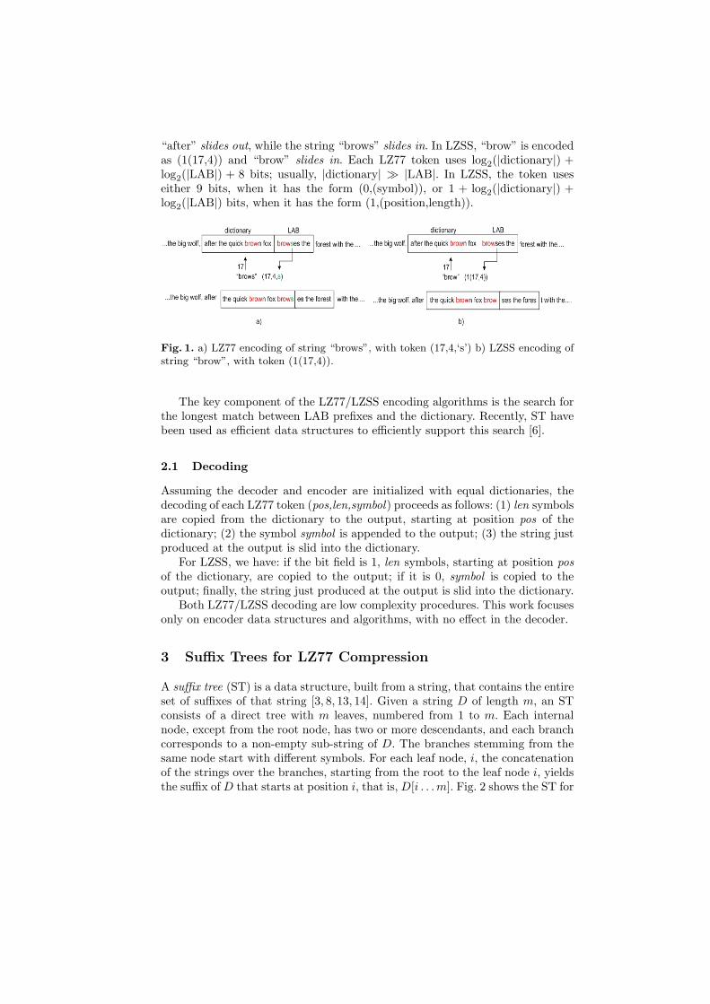
“after” slides out, while the string “brows” slides in. In LZSS, “brow” is encodedas (1(17,4)) and “brow” slides in. Each LZ77 token uses log

2(|dictionary|) +

log2(|LAB|) + 8 bits; usually, |dictionary| � |LAB|. In LZSS, the token uses

either 9 bits, when it has the form (0,(symbol)), or 1 + log2(|dictionary|) +

log2(|LAB|) bits, when it has the form (1,(position,length)).

Fig. 1. a) LZ77 encoding of string “brows”, with token (17,4,‘s’) b) LZSS encoding ofstring “brow”, with token (1(17,4)).

The key component of the LZ77/LZSS encoding algorithms is the search forthe longest match between LAB prefixes and the dictionary. Recently, ST havebeen used as efficient data structures to efficiently support this search [6].

2.1 Decoding

Assuming the decoder and encoder are initialized with equal dictionaries, thedecoding of each LZ77 token (pos,len,symbol) proceeds as follows: (1) len symbolsare copied from the dictionary to the output, starting at position pos of thedictionary; (2) the symbol symbol is appended to the output; (3) the string justproduced at the output is slid into the dictionary.

For LZSS, we have: if the bit field is 1, len symbols, starting at position posof the dictionary, are copied to the output; if it is 0, symbol is copied to theoutput; finally, the string just produced at the output is slid into the dictionary.

Both LZ77/LZSS decoding are low complexity procedures. This work focusesonly on encoder data structures and algorithms, with no effect in the decoder.

3 Suffix Trees for LZ77 Compression

A suffix tree (ST) is a data structure, built from a string, that contains the entireset of suffixes of that string [3, 8, 13, 14]. Given a string D of length m, an STconsists of a direct tree with m leaves, numbered from 1 to m. Each internalnode, except from the root node, has two or more descendants, and each branchcorresponds to a non-empty sub-string of D. The branches stemming from thesame node start with different symbols. For each leaf node, i, the concatenationof the strings over the branches, starting from the root to the leaf node i, yieldsthe suffix of D that starts at position i, that is, D[i . . . m]. Fig. 2 shows the ST for

string D = xabxa$, with suffixes xabxa$, abxa$, bxa$, xa$, a$ and $. Each leafnode contains the corresponding suffix number. In order to be possible to build

Fig. 2. Suffix Tree for string D = xabxa$. Each leaf node contains the correspondingsuffix number. Each suffix is obtained by walking down the tree, from the root node.

an ST from a given string, it is necessary that no suffix of smaller length prefixesanother suffix of greater length. This condition is assured by the insertion ofa terminator symbol ($) at the end of the string. The terminator is a specialsymbol that does not occur previously on the string [3].

3.1 Encoding Using Suffix Trees

An ST can be applied to obtain the LZ77/LZSS encoding of a file, as we showin Algorithm 1 [3].

Algorithm 1 - ST-Based LZ77 Encoding

Inputs: In, input stream to encode; m and n, length of dictionary and LAB.Output: Out, output stream with LZ77 description of In.

1. Read dictionary D and look-ahead-buffer LAB from In.2. While there are symbols of In to encode:

a) Build, in O(m) time, an ST for string D.b) Number each internal node v with cv, the smallest number of all the

suffixes in v’s subtree; this way, cv is the left-most position in D of anycopy of the sub-string on the path from the root to node v.

c) To obtain the description (pos, len) for the sub-string LAB[i . . . n], with0 ≤ i < n:c1) If no suffix starts with LAB[i], output (0, 0, LAB[i]) to Out and do

i← i + 1, and goto 2c6).c2) Follow the only path from the root that matches the prefix LAB[i . . . n].c3) The traversal stops at point p (not necessarily a node), when a sym-

bol breaks the match; let depth(p) be the length of the string fromthe root to p and v the first node at or below p.

c4) Do pos← cv and len← depth(p).c5) Output token (pos, len, LAB[j]) to Out, with j = i+len, do i← j+1.c6) if i = n goto 2d); else goto 2c).

d) Slide in the full encoded LAB into D;e) Read next LAB from In; goto 2).

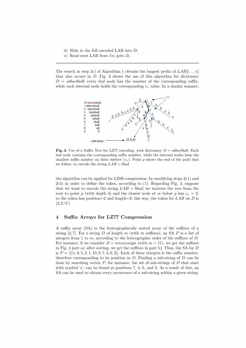
The search in step 2c) of Algorithm 1 obtains the longest prefix of LAB[i . . . n]that also occurs in D. Fig. 3 shows the use of this algorithm for dictionaryD = abbacbba$; every leaf node has the number of the corresponding suffix,while each internal node holds the corresponding cv value. In a similar manner,

Fig. 3. Use of a Suffix Tree for LZ77 encoding, with dictionary D = abbacbba$. Eachleaf node contains the corresponding suffix number, while the internal nodes keep thesmallest suffix number on their subtree (cv). Point p shows the end of the path thatwe follow, to encode the string LAB = bbad.

the algorithm can be applied for LZSS compression, by modifying steps 2c1) and2c5) in order to define the token, according to (1). Regarding Fig. 3, supposethat we want to encode the string LAB = bbad; we traverse the tree from theroot to point p (with depth 3) and the closest node at or below p has cv = 2,so the token has position=2 and length=3; this way, the token for LAB on D is(2,3,‘d’).

4 Suffix Arrays for LZ77 Compression

A suffix array (SA) is the lexicographically sorted array of the suffixes of astring [3, 7]. For a string D of length m (with m suffixes), an SA P is a list ofintegers from 1 to m, according to the lexicographic order of the suffixes of D.For instance, if we consider D = mississippi (with m = 11), we get the suffixesin Fig. 4 part a); after sorting, we get the suffixes in part b). Thus, the SA for D

is P = {11, 8, 5, 2, 1, 10, 9, 7, 4, 6, 3}. Each of these integers is the suffix number,therefore corresponding to its position in D. Finding a sub-string of D can bedone by searching vector P ; for instance, the set of sub-strings of D that startwith symbol ‘s’, can be found at positions 7, 4, 6, and 3. As a result of this, anSA can be used to obtain every occurrence of a sub-string within a given string.

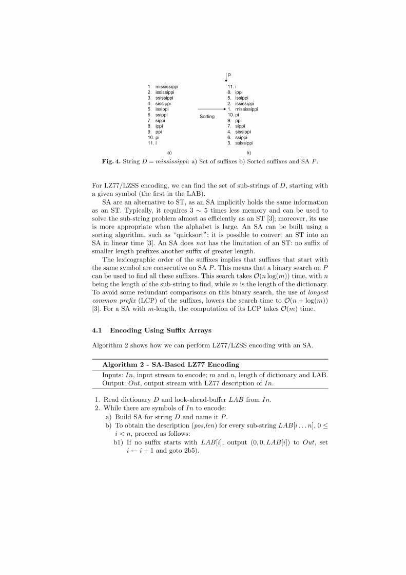
Fig. 4. String D = mississippi: a) Set of suffixes b) Sorted suffixes and SA P .

For LZ77/LZSS encoding, we can find the set of sub-strings of D, starting witha given symbol (the first in the LAB).

SA are an alternative to ST, as an SA implicitly holds the same informationas an ST. Typically, it requires 3 ∼ 5 times less memory and can be used tosolve the sub-string problem almost as efficiently as an ST [3]; moreover, its useis more appropriate when the alphabet is large. An SA can be built using asorting algorithm, such as “quicksort”; it is possible to convert an ST into anSA in linear time [3]. An SA does not has the limitation of an ST: no suffix ofsmaller length prefixes another suffix of greater length.

The lexicographic order of the suffixes implies that suffixes that start withthe same symbol are consecutive on SA P . This means that a binary search on P

can be used to find all these suffixes. This search takes O(n log(m)) time, with n

being the length of the sub-string to find, while m is the length of the dictionary.To avoid some redundant comparisons on this binary search, the use of longestcommon prefix (LCP) of the suffixes, lowers the search time to O(n + log(m))[3]. For a SA with m-length, the computation of its LCP takes O(m) time.

4.1 Encoding Using Suffix Arrays

Algorithm 2 shows how we can perform LZ77/LZSS encoding with an SA.

Algorithm 2 - SA-Based LZ77 Encoding

Inputs: In, input stream to encode; m and n, length of dictionary and LAB.Output: Out, output stream with LZ77 description of In.

1. Read dictionary D and look-ahead-buffer LAB from In.2. While there are symbols of In to encode:

a) Build SA for string D and name it P .b) To obtain the description (pos,len) for every sub-string LAB[i . . . n], 0 ≤

i < n, proceed as follows:

b1) If no suffix starts with LAB[i], output (0, 0, LAB[i]) to Out, seti← i + 1 and goto 2b5).

b2) Do a binary search on vector P until we find: the first position left,in which the first symbol of the corresponding suffix matches LAB[i],that is, D[P [left]] = LAB[i]; the last position right, in which thefirst symbol of the corresponding suffix matches LAB[i], that is,D[P [right]] = LAB[i].

b3) From the set of suffixes between P [left] and P [right], choose the kth

suffix, left ≤ k ≤ right, with a given criteria (see below) giving ap-length match.

b4) Do pos ← k, len ← p and i← i+len and output token (pos, len, LAB[i])into Out.

b5) If i = n goto 2c); else goto 2b).

c) Slide in the full encoded LAB into D;

d) Read next LAB from In; goto 2).

In step 2.b2), it is possible to choose among several suffixes, according to agreedy/non-greedy parsing criterion. If we seek a fast search, we can choose oneof the immediate suffixes, given by left or right. If we want better compressionratio, at the expense of a not so fast search, we should choose the suffix withthe longest match with sub-string LAB[i . . . n]. LZSS encoding can be done in asimilar way, by changing the token format according to (1).

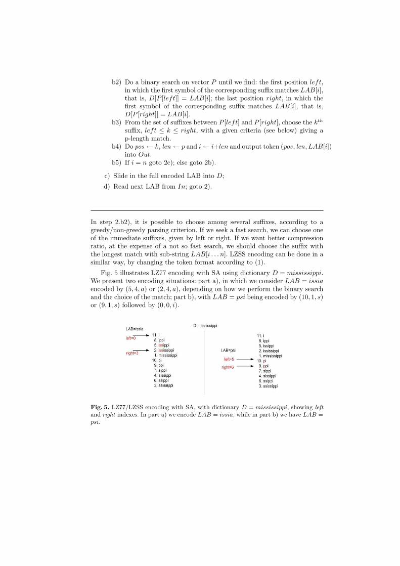
Fig. 5 illustrates LZ77 encoding with SA using dictionary D = mississippi.We present two encoding situations: part a), in which we consider LAB = issia

encoded by (5, 4, a) or (2, 4, a), depending on how we perform the binary searchand the choice of the match; part b), with LAB = psi being encoded by (10, 1, s)or (9, 1, s) followed by (0, 0, i).

Fig. 5. LZ77/LZSS encoding with SA, with dictionary D = mississippi, showing left

and right indexes. In part a) we encode LAB = issia, while in part b) we have LAB =psi.

5 Implementation Details

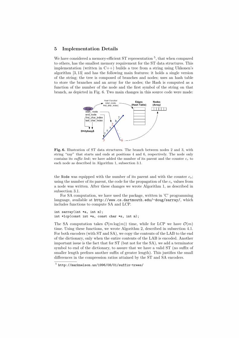
We have considered a memory-efficient ST representation 5, that when comparedto others, has the smallest memory requirement for the ST data structures. Thisimplementation (written in C++) builds a tree from a string using Ukkonen’salgorithm [3, 13] and has the following main features: it holds a single versionof the string; the tree is composed of branches and nodes; uses an hash tableto store the branches and an array for the nodes; the Hash is computed as afunction of the number of the node and the first symbol of the string on thatbranch, as depicted in Fig. 6. Two main changes in this source code were made:

Fig. 6. Illustration of ST data structures. The branch between nodes 2 and 3, withstring “xay” that starts and ends at positions 4 and 6, respectively. The node onlycontains its suffix link ; we have added the number of its parent and the counter cv toeach node as described in Algorithm 1, subsection 3.1.

the Node was equipped with the number of its parent and with the counter cv;using the number of its parent, the code for the propagation of the cv values froma node was written. After these changes we wrote Algorithm 1, as described insubsection 3.1.

For SA computation, we have used the package, written in ’C’ programminglanguage, available at http://www.cs.dartmouth.edu/~doug/sarray/, whichincludes functions to compute SA and LCP.

int sarray(int *a, int m);

int *lcp(const int *a, const char *s, int m);

The SA computation takes O(m log(m)) time, while for LCP we have O(m)time. Using these functions, we wrote Algorithm 2, described in subsection 4.1.For both encoders (with ST and SA), we copy the contents of the LAB to the endof the dictionary, only when the entire contents of the LAB is encoded. Anotherimportant issue is the fact that for ST (but not for the SA), we add a terminatorsymbol to end of the dictionary, to assure that we have a valid ST (no suffix ofsmaller length prefixes another suffix of greater length). This justifies the smalldifferences in the compression ratios attained by the ST and SA encoders.

5 http://marknelson.us/1996/08/01/suffix-trees/

6 Experimental Results

This section presents the experimental results of LZSS encoders, with dictionar-ies and LAB of different lengths. The evaluation was carried out using standardtest files from the well-known Calgary Corpus6 and Canterbury Corpus7. Wehave considered a set of 18 files, with a total size of 2680580 bytes: bib (111261bytes); book1 (768771 bytes); book2 (610856 bytes); news (377109 bytes); pa-per1 (53161 bytes); paper2 (82199 bytes); paper3 (46526 bytes); paper4 (13286bytes); paper5 (11954 bytes); paper6 (38105 bytes); progc (39611 bytes); progl(71646 bytes); progp (49379 bytes); trans (93695 bytes); alice29 (152089 bytes);asyoulik (125179 bytes); cp (24603 bytes); fields (11150 bytes).

The compression tests were executed on a machine with 2GB RAM and anIntel processor Core2 Duo CPU T7300 @ 2GHz. We measured the followingparameters: encoding time (in seconds), memory occupied by the encoder datastructures (in bytes) and compression ratio in bits per byte

bpb = 8Encoded Size

Original Size, (2)

for the LZSS encoder. The memory indicator refers to the average amount ofmemory needed for every ST and SA, built in the encoding process, given by

MST = |Edges|+ |Nodes|+ |dictionary|+ |LAB|,

MSA = |Suffix Array|+ |dictionary|+ |LAB|, (3)

for the ST encoder and SA encoder, respectively (the operator |.| gives thelength in bytes). Each ST edge is made up of 4 integers (see Fig. 6) and eachnode has 3 integers (suffix link, cv counter and parent identification, as describedin Section 5); each integer occupies 4 bytes. On the SA encoder tests, we haveconsidered the choice of k as the mid-point between left and right, as stated inAlgorithm 2 in subsection 4.1.

6.1 Encoding Time, Memory and Compression Ratio

We consider a small dictionary with length 128 and |LAB|=16 or |LAB|=32,as shown in Table 1 with the results for the 18 chosen files. We see that SAare slightly faster than ST, but achieve a lower compression ratio. The amountof memory for the SA encoder is fixed at 660 (=129*4 + 128 +16) and 676(=129*4 + 128 + 32). The amount of memory for the ST encoder is larger andvariable, because the number of edges and nodes depends on the suffixes of thestring in the dictionary. With small dictionaries, we have a low encoding time(fast compression) with a reasonable compression ratio. We conclude that theincrease of the LAB gives rise to a lower encoding time, for both ST and SAencoders. For |LAB|=32, the SA encoder is faster than the ST encoder, but thislast one attains a better compression ratio.

6 http://links.uwaterloo.ca/calgary.corpus.html7 http://corpus.canterbury.ac.nz/

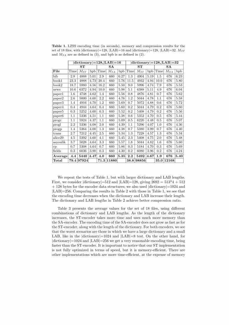
Table 1. LZSS encoding time (in seconds), memory and compression results for theset of 18 files, with |dictionary|=128, |LAB|=16 and |dictionary|=128, |LAB|=32. MST

and MSA are as defined in (3), and bpb is as defined in (2).

|dictionary|=128,|LAB|=16 |dictionary|=128,|LAB|=32

ST SA ST SA

File Time MST bpb Time MSA bpb Time MST bpb Time MSA bpb

bib 2.8 4888 5.01 2.9 660 6.27 1.3 4904 5.19 1.5 676 6.23

book1 23.3 4888 4.73 20.4 660 5.76 11.5 4932 4.94 10.0 676 5.80

book2 18.7 5980 4.56 16.2 660 5.50 9.0 5996 4.74 7.9 676 5.53

news 10.6 6372 4.94 10.0 660 5.98 5.1 6388 5.11 4.9 676 6.04

paper1 1.6 4748 4.62 1.4 660 5.56 0.8 4876 4.81 0.7 676 5.62

paper2 2.6 5000 4.60 2.2 660 4.76 1.2 5044 4.78 1.1 676 5.58

paper3 1.4 4916 4.70 1.2 660 5.69 0.7 5072 4.88 0.6 676 5.72

paper4 0.4 4944 4.64 0.4 660 5.60 0.2 5044 4.79 0.2 676 5.60

paper5 0.3 5252 4.60 0.3 660 5.52 0.2 5408 4.79 0.2 676 5.56

paper6 1.1 5336 4.51 1.1 660 5.38 0.6 5352 4.70 0.5 676 5.44

progc 1.1 5924 4.37 1.1 660 5.09 0.5 6220 4.48 0.5 676 5.07

progl 2.2 5336 4.08 2.0 660 4.39 1.1 5296 4.07 1.0 676 4.36

progp 1.4 5364 4.00 1.3 660 4.38 0.7 5380 3.99 0.7 676 4.40

trans 2.7 7212 4.45 2.5 660 5.34 1.3 7228 4.57 1.3 676 5.34

alice29 4.5 5392 4.60 4.1 660 5.45 2.3 5408 4.75 2.0 676 5.48

asyoulik 3.7 5028 4.64 3.3 660 5.57 1.8 5044 4.82 1.6 676 5.60

cp 0.7 5308 4.64 0.7 660 5.86 0.3 5184 4.70 0.3 676 5.69

fields 0.3 6036 3.90 0.3 660 4.30 0.2 6080 3.96 0.2 676 4.24

Average 4.4 5440 4.47 4.0 660 5.35 2.2 5492 4.67 1.9 676 5.40

Total 79.4 97924 71.3 11880 38.8 98856 35.0 12168

We repeat the tests of Table 1, but with larger dictionary and LAB lengths.First, we consider |dictionary|=512 and |LAB|=128, giving 2692 = 513*4 + 512+ 128 bytes for the encoder data structures; we also used |dictionary|=1024 and|LAB|=256. Comparing the results in Table 2 with those in Table 1, we see thatthe encoding time decreases when the dictionary and LAB increase their length.The dictionary and LAB lengths in Table 2 achieve better compression ratio.

Table 3 presents the average values for the set of 18 files, using differentcombinations of dictionary and LAB lengths. As the length of the dictionaryincreases, the ST-encoder takes more time and uses much more memory thanthe SA-encoder. The encoding time of the SA-encoder does not grow as fast as forthe ST-encoder, along with the length of the dictionary. For both encoders, we seethat the worst scenarios are those in which we have a large dictionary and a smallLAB, like in the |dictionary|=1024 and |LAB|=8 test. On the other hand, for|dictionary|=1024 and |LAB|=256 we get a very reasonable encoding time, beingfaster than the ST-encoder. It is important to notice that our ST implementationis not fully optimized in terms of speed, but it is memory-efficient. There areother implementations which are more time-efficient, at the expense of memory

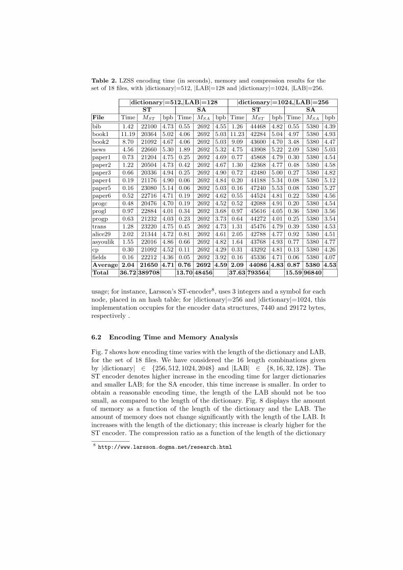
Table 2. LZSS encoding time (in seconds), memory and compression results for theset of 18 files, with |dictionary|=512, |LAB|=128 and |dictionary|=1024, |LAB|=256.

|dictionary|=512,|LAB|=128 |dictionary|=1024,|LAB|=256

ST SA ST SA

File Time MST bpb Time MSA bpb Time MST bpb Time MSA bpb

bib 1.42 22100 4.73 0.55 2692 4.55 1.26 44468 4.82 0.55 5380 4.39

book1 11.19 20364 5.02 4.06 2692 5.03 11.23 42284 5.04 4.97 5380 4.93

book2 8.70 21092 4.67 4.06 2692 5.03 9.09 43600 4.70 3.48 5380 4.47

news 4.56 22660 5.30 1.89 2692 5.32 4.75 43908 5.22 2.09 5380 5.03

paper1 0.73 21204 4.75 0.25 2692 4.69 0.77 45868 4.79 0.30 5380 4.54

paper2 1.22 20504 4.73 0.42 2692 4.67 1.30 42368 4.77 0.48 5380 4.58

paper3 0.66 20336 4.94 0.25 2692 4.90 0.72 42480 5.00 0.27 5380 4.82

paper4 0.19 21176 4.90 0.06 2692 4.84 0.20 44188 5.34 0.08 5380 5.12

paper5 0.16 23080 5.14 0.06 2692 5.03 0.16 47240 5.53 0.08 5380 5.27

paper6 0.52 22716 4.71 0.19 2692 4.62 0.55 44524 4.81 0.22 5380 4.56

progc 0.48 20476 4.70 0.19 2692 4.52 0.52 42088 4.91 0.20 5380 4.54

progl 0.97 22884 4.01 0.34 2692 3.68 0.97 45616 4.05 0.36 5380 3.56

progp 0.63 21232 4.03 0.23 2692 3.73 0.64 44272 4.01 0.25 5380 3.54

trans 1.28 23220 4.75 0.45 2692 4.73 1.31 45476 4.79 0.39 5380 4.53

alice29 2.02 21344 4.72 0.81 2692 4.61 2.05 42788 4.77 0.92 5380 4.51

asyoulik 1.55 22016 4.86 0.66 2692 4.82 1.64 43768 4.93 0.77 5380 4.77

cp 0.30 21092 4.52 0.11 2692 4.29 0.31 43292 4.81 0.13 5380 4.26

fields 0.16 22212 4.36 0.05 2692 3.92 0.16 45336 4.71 0.06 5380 4.07

Average 2.04 21650 4.71 0.76 2692 4.59 2.09 44086 4.83 0.87 5380 4.53

Total 36.72 389708 13.70 48456 37.63 793564 15.59 96840

usage; for instance, Larsson’s ST-encoder8, uses 3 integers and a symbol for eachnode, placed in an hash table; for |dictionary|=256 and |dictionary|=1024, thisimplementation occupies for the encoder data structures, 7440 and 29172 bytes,respectively .

6.2 Encoding Time and Memory Analysis

Fig. 7 shows how encoding time varies with the length of the dictionary and LAB,for the set of 18 files. We have considered the 16 length combinations givenby |dictionary| ∈ {256, 512, 1024, 2048} and |LAB| ∈ {8, 16, 32, 128}. TheST encoder denotes higher increase in the encoding time for larger dictionariesand smaller LAB; for the SA encoder, this time increase is smaller. In order toobtain a reasonable encoding time, the length of the LAB should not be toosmall, as compared to the length of the dictionary. Fig. 8 displays the amountof memory as a function of the length of the dictionary and the LAB. Theamount of memory does not change significantly with the length of the LAB. Itincreases with the length of the dictionary; this increase is clearly higher for theST encoder. The compression ratio as a function of the length of the dictionary

8 http://www.larsson.dogma.net/research.html

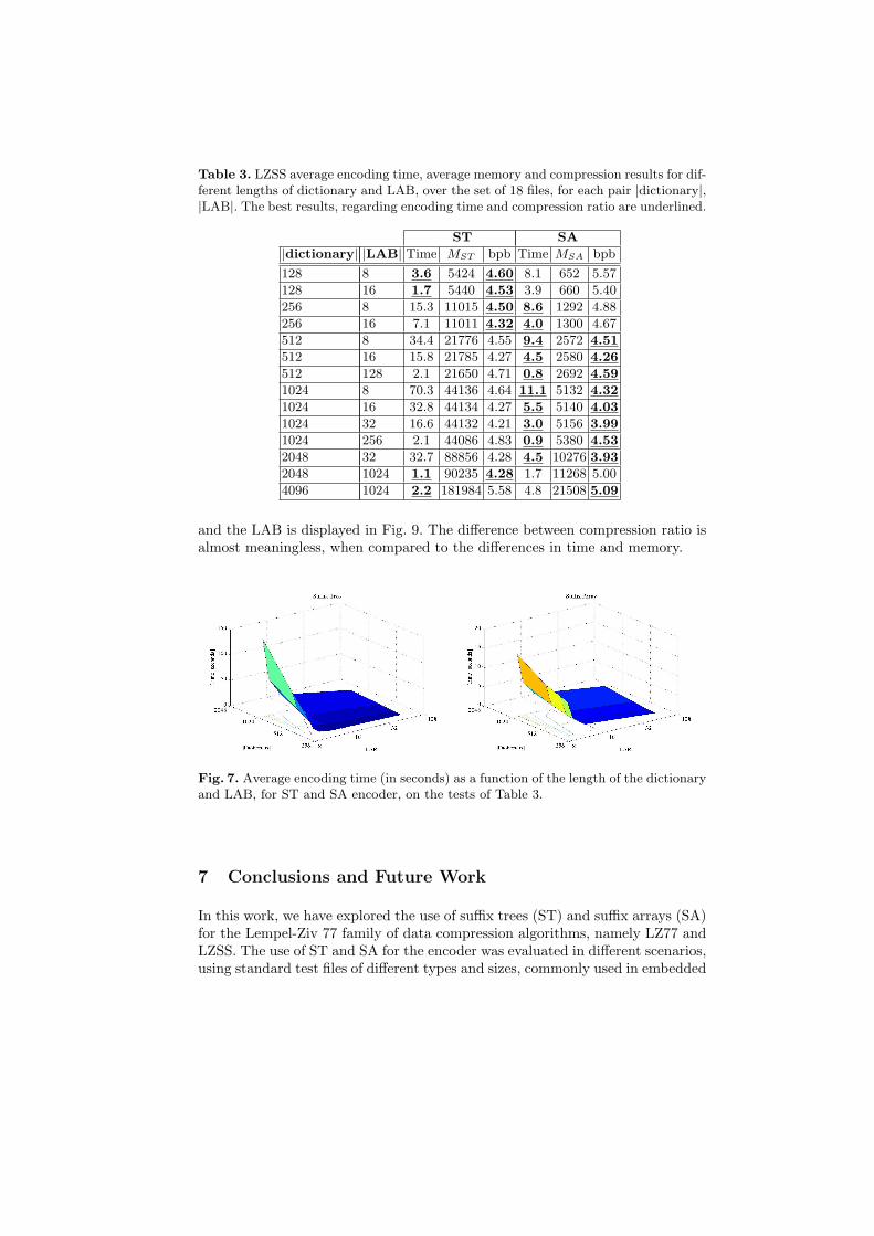
Table 3. LZSS average encoding time, average memory and compression results for dif-ferent lengths of dictionary and LAB, over the set of 18 files, for each pair |dictionary|,|LAB|. The best results, regarding encoding time and compression ratio are underlined.

ST SA

|dictionary| |LAB| Time MST bpb Time MSA bpb

128 8 3.6 5424 4.60 8.1 652 5.57

128 16 1.7 5440 4.53 3.9 660 5.40

256 8 15.3 11015 4.50 8.6 1292 4.88

256 16 7.1 11011 4.32 4.0 1300 4.67

512 8 34.4 21776 4.55 9.4 2572 4.51

512 16 15.8 21785 4.27 4.5 2580 4.26

512 128 2.1 21650 4.71 0.8 2692 4.59

1024 8 70.3 44136 4.64 11.1 5132 4.32

1024 16 32.8 44134 4.27 5.5 5140 4.03

1024 32 16.6 44132 4.21 3.0 5156 3.99

1024 256 2.1 44086 4.83 0.9 5380 4.53

2048 32 32.7 88856 4.28 4.5 10276 3.93

2048 1024 1.1 90235 4.28 1.7 11268 5.00

4096 1024 2.2 181984 5.58 4.8 21508 5.09

and the LAB is displayed in Fig. 9. The difference between compression ratio isalmost meaningless, when compared to the differences in time and memory.

Fig. 7. Average encoding time (in seconds) as a function of the length of the dictionaryand LAB, for ST and SA encoder, on the tests of Table 3.

7 Conclusions and Future Work

In this work, we have explored the use of suffix trees (ST) and suffix arrays (SA)for the Lempel-Ziv 77 family of data compression algorithms, namely LZ77 andLZSS. The use of ST and SA for the encoder was evaluated in different scenarios,using standard test files of different types and sizes, commonly used in embedded

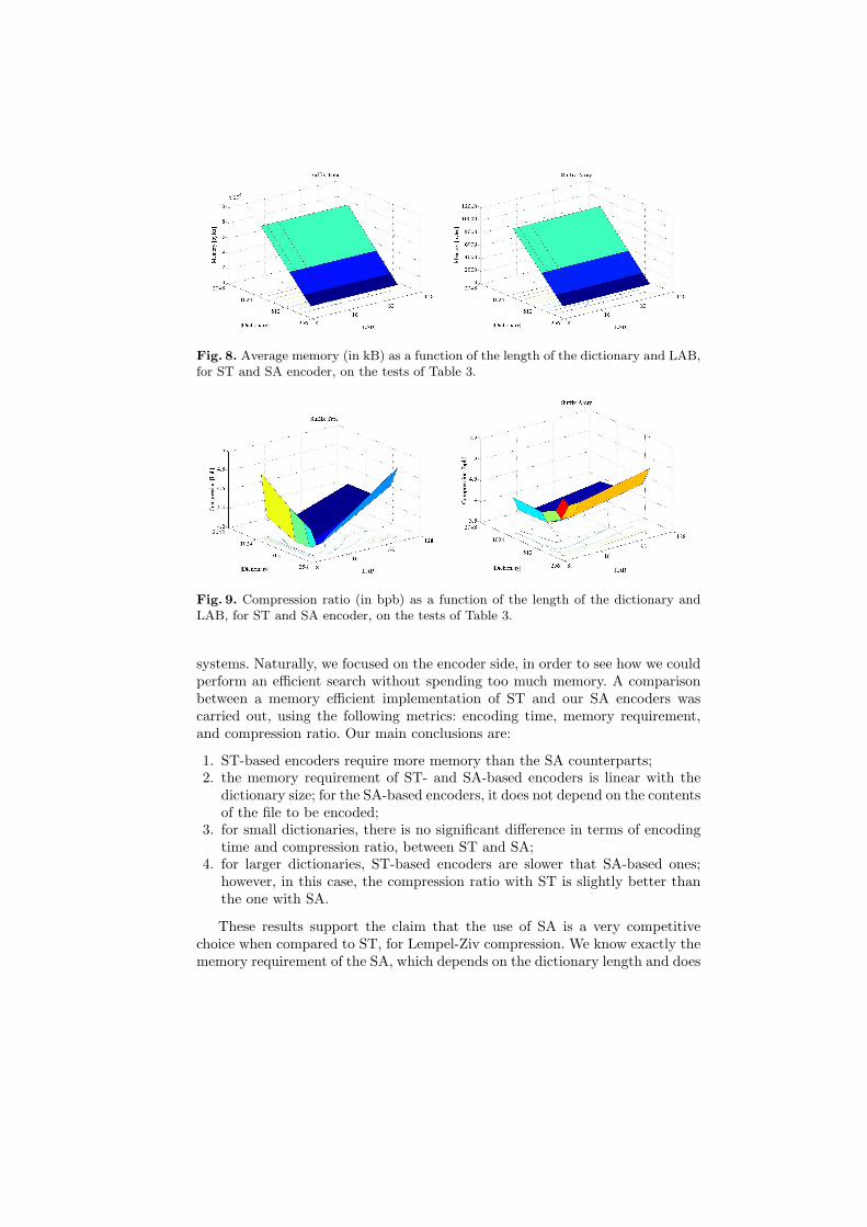
Fig. 8. Average memory (in kB) as a function of the length of the dictionary and LAB,for ST and SA encoder, on the tests of Table 3.

Fig. 9. Compression ratio (in bpb) as a function of the length of the dictionary andLAB, for ST and SA encoder, on the tests of Table 3.

systems. Naturally, we focused on the encoder side, in order to see how we couldperform an efficient search without spending too much memory. A comparisonbetween a memory efficient implementation of ST and our SA encoders wascarried out, using the following metrics: encoding time, memory requirement,and compression ratio. Our main conclusions are:

1. ST-based encoders require more memory than the SA counterparts;2. the memory requirement of ST- and SA-based encoders is linear with the

dictionary size; for the SA-based encoders, it does not depend on the contentsof the file to be encoded;

3. for small dictionaries, there is no significant difference in terms of encodingtime and compression ratio, between ST and SA;

4. for larger dictionaries, ST-based encoders are slower that SA-based ones;however, in this case, the compression ratio with ST is slightly better thanthe one with SA.

These results support the claim that the use of SA is a very competitivechoice when compared to ST, for Lempel-Ziv compression. We know exactly thememory requirement of the SA, which depends on the dictionary length and does

not depend on the text to encode. In application scenarios where the length ofthe dictionary is medium or large and the available memory is scarce and speedis not so important, it is preferable to use SA instead of ST. This way, SAare suited for this purpose, regarding the trade-off between time, memory, andcompression ratio, being preferable for mobile devices and embedded systems.

As ongoing and future work, we are developing two new faster SA-basedalgorithms. The first algorithm updates the indexes of the unique SA, built atthe beginning of the encoding process, after each full look-ahead-buffer encoding.The idea is that after each look-ahead-buffer encoding, the dictionary is closelyrelated to the previous one; this way, regarding the dictionary data structureswe need only to update an array of integers. The second algorithm uses longestcommon prefix to get the length field of the token; this version will be more costlyin terms of memory, but it should run faster than all the other SA-encoders.

References

1. Abouelhoda, M., Kurtz, S., and Ohlebusch, E. (2004). Replacing suffix trees withenhanced suffix arrays. Journal of Discrete Algorithms, 2(1):53–86.

2. Fiala, M. and Holub, J. (2008). DCA using suffix arrays. In Data Compression

Conference DCC2008, page 516.3. Gusfield, D. (1997). Algorithms on Strings, Trees and Sequences. Cambridge Uni-

versity Press.4. Karkainen, J., Sanders, P., and S.Burkhardt (2006). Linear work suffix array con-

struction. Journal of the ACM, 53(6):918–936.5. Larsson, N. (1996). Extended application of suffix trees to data compression. In

Data Compression Conference, page 190.6. Larsson, N. (1999). Structures of String Matching and Data Compression. PhD

thesis, Department of Computer Science, Lund University, Sweden.7. Manber, U. and Myers, G. (1993). Suffix arrays: a new method for on-line string

searches. SIAM Journal on Computing, 22(5):935–948.8. McCreight, E. (1976). A space-economical suffix tree construction algorithm. Jour-

nal of the ACM, 23(2):262–272.9. Sadakane, K. (2000). Compressed text databases with efficient query algorithms

based on the compressed suffix array. In ISAAC’00, volume LNCS 1969, pages 410–421.

10. Salomon, D. (2007). Data Compression - The complete reference. Springer-VerlagLondon Ltd, London, fourth edition.

11. Sestak, R., Lnsk, J., and Zemlicka, M. (2008). Suffix array for large alphabet. InData Compression Conference DCC2008, page 543.

12. Storer, J. and Szymanski, T. (1982). Data compression via textual substitution.Journal of ACM, 29(4):928–951.

13. Ukkonen, E. (1995). On-line construction of suffix trees. Algorithmica, 14(3):249–260.

14. Weiner, P. (1973). Linear pattern matching algorithm. In 14th Annual IEEE

Symposium on Switching and Automata Theory, volume 27, pages 1–11.15. Zhang, S. and Nong, G. (2008). Fast and space efficient linear suffix array con-

struction. In Data Compression Conference DCC2008, page 553.16. Ziv, J. and Lempel, A. (1977). A universal algorithm for sequential data compres-

sion. IEEE Transactions on Information Theory, IT-23(3):337–343.