R 81 Philips Res. Rep. 3, 213-226, 1948

ON THE THEORY OF COUPLED ANTENNAE

by C. J. BOUWKAMP 621.396.671

Summary

The purpose of this paper is to provide formulae for the self andmutual impedances of rui antenna system consisting of two identical,centre-fed, parallel, cylindrical wires. Tables of auxiliary functionsare given facilitating numerical investigation in the range1 < 2nljJ.. < 2, 0 < djl < 2, n = 2 ln(2lja) > 10, where 2l isthe length of each antenna, d their mutual distance, 2a the wirediameter, and Ä the wavelength. Examples illustrating the generaltheory are deferred to a subsequent paper.

JRésumé

L'objet de cet article est de fournir des formules pour les impédancespropre et mutuelle d'un système d'antennes constitué par deux mincesbrins identiques, parallèles, cylindriques, alimentës au centre. L'ar-ticle comporte des tableaux de fonctions auxiliaires permettant defaire des investigations numériques dans la gamme 1 < 2nlj Ä < 2,o < djl < 2, n = 2 ln(2lja) > 10, oil 2l est la longueur de chaqueantenne, d leur distance mutuelle, 2a Ie diamètre du fil et Ä la Ion-gueur d'onde. Les exemples d'application de la thëorie gënërale sontréservés à un article suivant.

1. Introduction

As is ohvious from first principles of electrpmagnetic theory, the radiationproperties of a transmitting antenna ultimately depend on and are deter-mined by the distribution of current and charge. Once the currents andcharges are known, the electromagnetic :field is easily obtained by the"classical method of vector and scalar potentials. Therefore, an adequatestarting point in the theory of antenna radiation is to assume the currentsand charges, that is, to consider them as given functions of time and posi-tion. In fact the older theories are all based upon this method, apartfrom a very few exceptions. Of course the theoretical results so obtainedmay be expected to agree fairly well with experiments if, and only if, theassumed sources are good approximations of the actual ones.The quasi-stationary theory often leads to useful approximations for the

currents and charges. It is then customary to calculate the actual cur-rents and charges approximately, by first neglecting the effect of radiation.As a consequence, in the development to shorter waves there is a generaltrend to extrapolate such important concepts as capacitance and inductanceto the ultra-high-frequency technique of to-day. On the other hand, the"electrical engineer is well aware that he has often to return to more funda-mental principles, that is, to Maxwell's equations ofthe electromagnetic field.

'214 C. J. BOUWKAMP

In this connection the antenna theory provides a striking example. Thedistribution of current in an isolated, centre-driven, cylindrical antenna wasformerly assumed to be sinusoidal, and this assumption is quite sound, aspointed out by various investigators 1),2),3),4). Though only the refinedtheory is able to treat satisfactorily such topics as anti-resonance, wherethe impedance is very large and highly dependent on the thickness of thewire, other corrections are usually small and almost negligible in practice.However, there are other examples which show that the older theories donot suffice at all "], 6). The calculation of the self and mutual impedancesof an antenna system in resonance is usually based on the assumption thatthe current along any of the conductors, whether driven or parasitic, is thesame as that along a free centre-driven antenna of the same dimensions.This assumption is not justifiable, On the contrary, especially for non-resonance, the current distribution in a receiving antenna placed in a homo-geneous field is not equal to that of the same antenna when used as trans-mitter, let alone that a loaded or unloaded parasitic antenna located in theneighbourhood of the driven antenna would show the same current distri-bution as the driven one. Furthermore, one should be careful in phase rea-soning for coupled antennae because, in the neighbourhood of the trans-mitting antenna, space differences have little to do with phase differences:At any rate, the relationship between phase changes and distances travelledis completely different from that existing in the wave zone.

Since a rigorogs- theory of the electromagnetic coupling of antennaeshould he able to provide us with data concerning input resistance at reso-nance, resonance shortening, etc., there is only one way to choose: one hasto return to the fundamentals of electromagnetic theory - it is not so_simple as to assume "convenient" currents; rather, the currents mustfirst be calculated.The present paper contains some results of a laboratory report 5) the

publication of which has been delayed by the war. That report dealt withthe radiation properties of the simplest case of the Yagi antenna, the systemconsisting of a centre-fed, straight wire in the presence of an unloaded para-sitic antenna parallel to and not displaced in length with respect to the.driven conductor (both wires being thin cylinders of equal cross-sections. andlengths, and of perfectly conducting material).. In passing we remark that following upon Hallén's fundamental contri-bution to antenna theory 1) numerous investigations were published byRonold King and collaborators. One of their papers 6) bears a close relationto the present report. However, since some of our results are either givendifferently or not dealt with by these authors, the present publication mayhe justified. .. The basic ideas and methods developed here are similar to thçse of a

THEORY OF COUPI,ED ANTENNAE

former paper 3). Characteristic of the Hallén problems is the appearance ofthe large parameter Q = 2 In (2lja), where 2l and 2n are respectively thelength and the diameter of the wires. Whereas in 3) terms of the order Q-2were included, here we take into account only terms of the order Q-l;otherwise the mathematics would become too involved.Finally, the present paper is devoted to the general outlines ofthe theory,

numerical applications being postponed to a subsequent report.

2. Formn1ation in terms of the vector potentia]

Let d denote the distance between two identical, parallel, cylindricalwires, both of length 2l and diameter 2a (l ~ a, d ~ a), the line connectingthe centres being perpendicular to both wires. The latter are centre-fed byslice generators of driving potential differences VI and V2 *). Furthermore,the two wires are supposed to be perfectly conducting. By virtue of thesymmetry in the feeding, the current distribution is symmetrical withrespect to z, where z denotes the distance along either antenna measuredfrom the corresponding centre. Let II(z) and 12(z) stand for the currents,which we may suppose to flow at the surfaces of the wires. These currentsare subjected to the condition that the resulting tangential electric fieldshall vanish at the surface of both wires. Alternative formulations of theproblem are (i) the currents flow at the surfaces of the cylinders supposedto he hollow, while the electric field vanishes on the two axes, and (ii) thecurrents are flowing in the axes, while the axial electric field vanishes atdistances a from the axes. These three different interpretations are equiva-lent when effects of the order afl are neglected 3).'Let IPll(z) denote the axial component ofthe vector potential on theaxis

of the first antenna as due to its own current, II(z). Let further IP21(Z)be the same component due to the current 12(z) flowing in the secondantenna. The functions IPI2(Z) and IP22(Z) are defined similarly. Then, uponintroducing ~2 = (z-C)2 + a2, R2 = (Z-C)2 + d2, we h~ve **)

.~.*) As usual, the discussion is confined to harmonic vibrations of frequency wl2n; th~

time dependence is exp(jwt).' . .' \.**) eisthe velocity oflight, k the wavenumber (k = wie = 27(,1}." where'á is the wavelength

in free space). Gaussian units are used throughout. '

215

(I)

216 C.J. BOUWKAMP

The axial components of the electric field due to the currents ·I1(z)and 1

2(z), at the axes of the antennae, can be found by differentiation

according to .

jkE(z) = (::2 + k2) (9'11 + 9121)'

jkE(z) = (!:+ k2) (9'12 + 9122)'•

for the first and for the second wire respectively. NowE (z) must vanishalongthe corresponding antenna, except at the centre, where it must cancel theimpressed electromotive force. In terms of the delta function we may thuswrite

Moreover, as the 91-functionsare symmetrical in z, we have by integration

9'l1(Z) + 9121(Z)=- i~V1 s~ klzl + Al cos kz 2,2 _LzI ~ l (2)9'12(Z)+ 9122(Z)=- i JV2 sm klzl + A2 cos kz , S

where the constants of integration, Al and A2' will he determined later on.

3. Approximate integral equations for the currents, and their solution

Analogous to the reasoning of paper 3), the functions 9'l1(Z) and 9122(z)are approximately proportional to the corresponding current distributions,viz.:

(3)

and its analogue for 9122(z) obtained when 11is replacedby 12•Ashefore 3),,Q(z) is an abbreviation for

fl de (~),Q(z.) = - ~n+ ln 1- - ,z -=1= 1.r •• l2-I

We thus obtain from (1), (2), (3):

(4)

THEORY OF COUPLED ANTENNAE 217

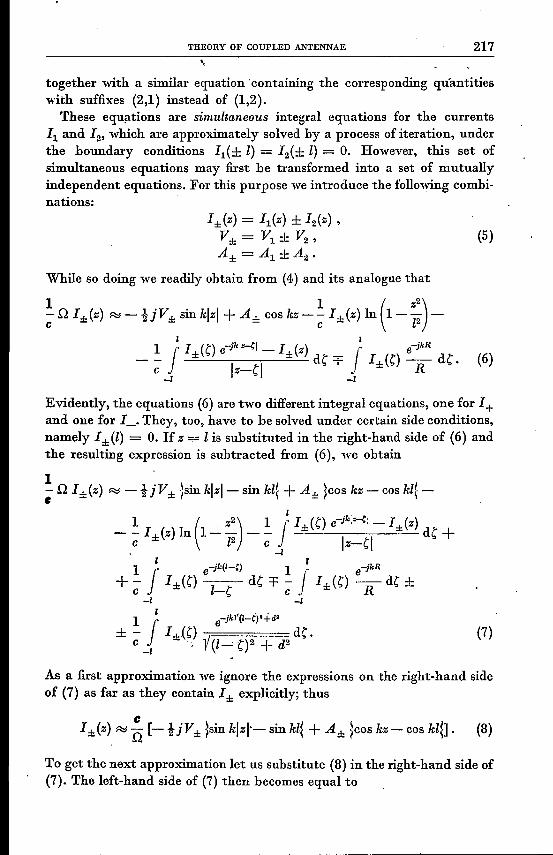
"together with a similar equation containing the corresponding quantitieswith suffixes (2,1) instead of (1,2).

These equations are simultaneous integral equations for the currents11and 12,which are approximately solved by a process of iteration, underthe boundary conditions 11(± 1) = 12(± 1) = O. However, this set ofsimultaneous equations may first be transformed into a set of mutuallyindependent equations. For this purpose we introduce the following combi-nations:

1±(z) = 11(z) ± 12(z) ,V± = V1 ± V2,A± = A1±A2•

While so doing we readily ohtain from (4) and its analogue that

(5)

1 1 (Z2)-.Q1±(z) ~-tjV±sinklzl+A±coskz--1±(z)ln 1---c c P

1 I1I (C) e-jk~1 - I (z) j~ e-jkR

- - ± I I ± dC T I± (C) -R dC.c z-C-I -I

(6)

Evidently, the equations (6) are two different integral equations, one for 1+and one for 1_. They, too, have to be solved under certain side conditions,namely 1±(1) = O. If z -- 1 is substituted in the right-hand side of (6) andthe resulting expression is subtracted from (6), 'we obtain

As a :first approximation we ignore the expressions on the right-hand sideof (7) as far as they contain I± explicitly; thus

e1±(z) ~ .Q [- t jV± ~sinklzl-- sin kl~+ A± ~coskz - cos klU. (8)

To get the next approximation let us substitute (8) in the right-hand side of(7). The left-hand side of (7) then becomes equal to

218 C• .T. BOUWKAlIIP

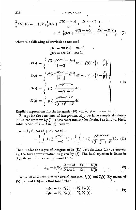
~ QI±(z) =-:-t iv; ~f(z) + F(l) ~F(z) ± H(l) ~H(z)~ +4. S G(l) - G(z) K(l) -K(z) 2+ ~± (g(z) + Q ± Q S' (9)

where the following abbreviations are used:

f(z) = sin klzl- sin kl,g(z) = cos kz - cos kl,

F(z) = /~f(C) e-jk:=-Cl - f(z) dC + f(z) In (1 _ z2.),. Iz-CI l2-I

f~g(C) e-jk:=-c, __: g(z) (Z2)G(z) = ~ Iz-CI dC + g(z) In 1 -P: ,

-I(10)

Explicit expressions for the integrals (10) will be given in section 5.Except for the constants of integration, A±, we have completely deter-

mined the currents by (9). These constants can be obtained as follows. First~substitution of z = l in (6) leads to )

o = - t jV ± sin kl + A± cos kl -1 r' e-jk(H) 1 f' e-jk."'(I-Cf·+di

- - I ± (C) " - -'_ dC =f - I ± (C) l" " de·c ., l-C e l (l-C)2 + d2-I -I

(11)

.Then, under the signs of integration in (11) we substitute for the currentI ± the first approximation as given by (8). The final equation is linear inA±; its solution is readily found to be "

. Q sin kl - F(l) =f H(l)A± = t,V± Q ~os kl- G(l) =f K(l)· (12)

We shall now return to the actual currents, Il(z) and 12('~). By means of(5), (9) and (12).is is thus found that ~

Il(z) = V1Yo(z) + V2 Ym(z),Iz(z) = V1Ym(z) + Vz Yo (z),

(13)

THEORY OF COUPLED ANTENNAE 219

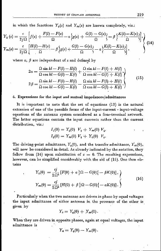
in which the functions Yo(z) and Ym(z) are known completely, viz.:

y. ( ) c [. F(l) -F(z) ~ G(l) - G(z) ~K(l)-K(z)~] ~o z = -.- j(z) + -a g(z) + i. - fJ '~Q Q 0 ) Q

(14)Y z)=_C_[I:l(l)-H(Z) ~nz G(l)-G(z)~_ SK(l)-K(Z)l] .m( 2'0 Q fJ(o() + 0 ) a ( 0 ~'J .

where a, fJare independent of zand define_dby

o sin kl- F(l) - H(l) Q sin kl- F(l) + H(l) ~2a = Q cos kl- G(l) - K(I) + Q cos kl- G(l) + K(l) ,

(15)Q sin kl- F(l) - H(l) Q sin kl- F(l) +H(l)

2fJ= Q cos kl- G(l) -K(l) - D. cos kl- G(l) + K(l) ,

4. Expressions for the input and mutual Impedancesfadmittances

It is important to note that the set of equations (13) is the naturalextension of one of the possible forms of the input-current - input-voltageequations of the antenna system considered as a four-terminal network.The latter equations contain the input currents rather than the currentdistribution, viz.:

.lI(O) = Yo(O) VI + Ym(O) V2,

12(0) = Ym(O) VI + Yo(O) V2•

The driving-point admittance, Yo(O), and the transfer admittance, Ym(O),will now be considered in detail. As already indicated by the notation, theyfollow from (14) upon suhstitution of z = O. The resulting expressions,however, can be simplified considerably with the aid of (15). One then ob-tains

Yo(O) = 2%2 [F(O) + a ~Q- G(O)~ - fJK(O)], tYm(O) = 2%2 [H(O) + fJ~Q - G(O) ~- aK(O)]. ~

(16)

Particularly when the two antennae are driven in phase by equal voltagesthe input admittance of either antenna in the presen~e of the other isgiven by

Ys = Yo(O) + Ym(O) .

When they are driven in opposite phases, again at equal voltages, the inputadmittance is' .

Ya = Yo(O) - Ym(O) .

220 C, J, BOUWKAMP

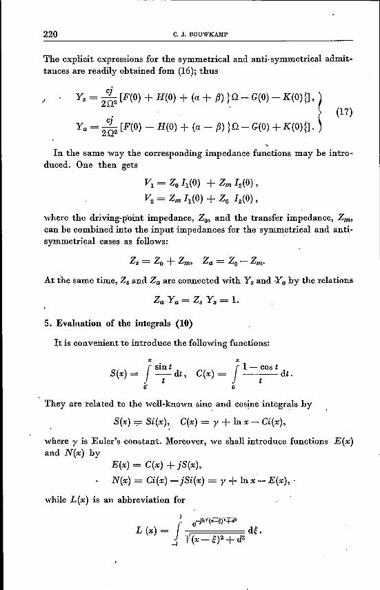
The explicit expressions for the symmetrical and anti-symmetrical admit-tances are readily obtained fom (16); thus

I Ys = 2;2 [F(O) + H(O) + (a + {3) ~,.Q- G(O) - K(O) n, !(17)

v, = 2;2 [F(O) - H(O) + (a - {3) ).Q - G(O) + K(O) U·In the same way the corresponding impedance functions may be intro-

duced. One then gets

VI = Zo 11(0) + z.; 12(0) ,V2 = z; 11(0) + Zo 12(0),

where the driving-point impedance, Zo, and the transfer impedance, Zm,can be combined into the input impedances for the symmetrical and anti-symmetrical cases as follows:

Zs = Zo + Zm, Za = Zo - Zm'

At the same time, Zs and Za are connected with Ys and :Ya by the relations

5. Evaluation of the integrals (10)

It is convenient to introduce the following functions:

~ ~

(' sin t (' 1 - cos tS(x) = - dt, C(x) = dt.

• t • tf 0

They are related to the well-known sine, and cosine integrals by

S(x) -::- Si(x), C(x) = y + In x - Ci(x),

where y is Euler's constant. Moreover, we shall introduce functions E(x)and N(x) by

E(x) = C(x) + jS(x),

N(x) = Ci(x) - jSi(x) = y + Inx - E(x), '

while L(x) is an abbreviation for

THEORY OFCOUPLED ANTENNAE 221

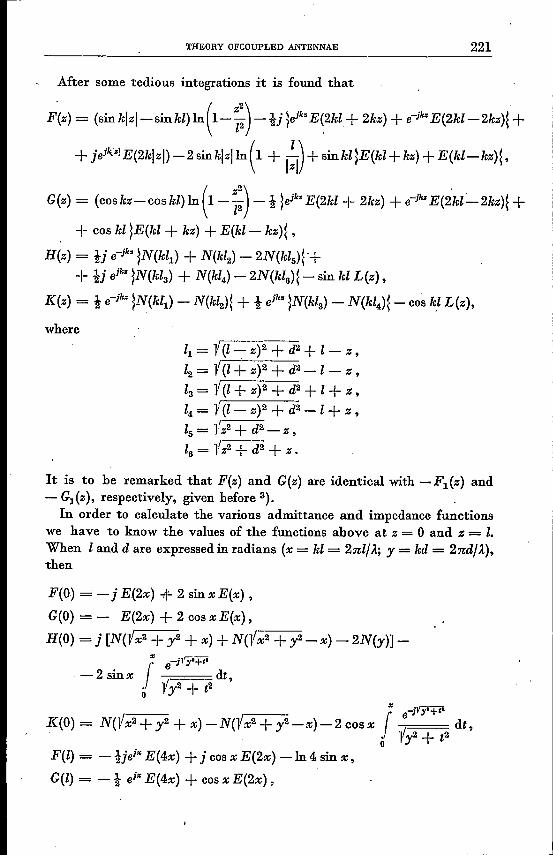
After some tedious integrations it is found that

FO(z)= (Sinklzl-sinkl)ln(1- ~:)-!i~eikzE~2kl + 2kz) + e-ikzE(2kl-2kz)~+

+ jeik~'lE(2klzD-2Sinklzlln(1 + 1~1)+SinkqE(kl+kZ)+E(kl-kzH,

G(z) = (coskz-cos kl) In(1-~:)- i ~eikzE(2kl + 2kz) + e-ik•E(2k(-2kz)~ +

-I- cos kl ~E(kl + kz) + E(kl- kzH '

H(z) = ij e-ik• ~N(k~) + N(k12) - 2N(kls)("++ ij eik. ~N(kla) + N(kl4) - 2N(k16H - sin kl L(z),

K(z) = !e-ik• ~N(krl) - N(kI2)( + i eik. ~N(kla) - N(kI4H - cos ~l L(z),

wheret --

II = l' (I - Z)2 + d2 + l - Z,l2= "V(I + z)2.f=d2 - l - z,la = "V(l + z)2 + d2+ l + Z,14= i(I - Z)2 + d2 - 1+ Z,

Ils = lZ2+ d2 - Z ,16 = yz2 + d2 + z.

It is to be remarked that F(z) and G(z) are identical with -FI(z) and- G] (z), respectively, given before a).In order to calculate the various admittance and impedance functions

we have to know the values of the functions above at z = 0 and z = 1.When I and d are expressed in radians (x = kl = 2n1!J..; y = kd = 2nd!J..),then

F(O) == - j E(2x) + 2 sin x E(x) ,

G(O) = - E(2x) + 2 cos x E(x),H(O) = j [Not x2 + y2 + x) + N(i x-2-+-y-2- x) - 2N(y)] -

- 2 sin x J'" e;-iJ

'?+!' dt,o 1y2 + t2

'" _jl'yl+,1

]((0) = N(ix2 + y2 + x) -N("VX2 + y2 -x) -2 cosx f le dt,o 0 1y2 + t2

F(l) = - Hei'" E(4x) + j cos x E(2x) -In 4 sin x,

G(l) = - i ei" E(4x) + cos x E(2x),

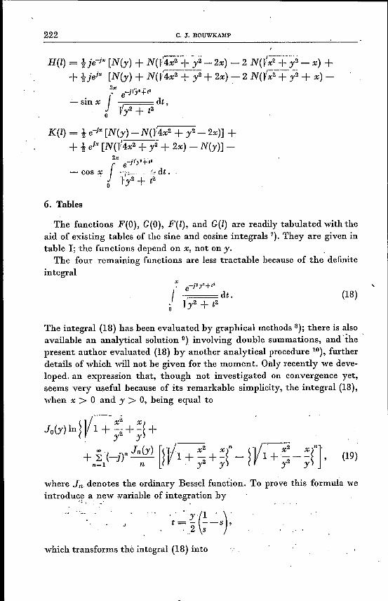
222 C. J. BOUWKAMP

H(l) = t je-jx [N(y) + N(l'4x2 + y2 - 2x) - 2 N(lfx2 + y2 - x) ++ tjejx [N(y) + N(t4x2 + y2+ 2x) --:-2 N(ix2 + y2 + x)-

2x r- ~

• e-j1y'+"- sin x J I ,dt ,

o ly2 + t2

K(l) = t e-jx [N(y) -N(l'4x2 + y2 - 2x)] ++ t ei·« [N(i4x2 + y2 + 2x) - N(y)]-

2.« -jt'y'-t',.

- cos ~ f 1~y2'+. '~ dt .o . .

6. Tables

The functions F(O), G(O), F(l), and G(l) are readily tabulated with theaid of existing tables of the sine and cosine integrals 7). They are given intable T; the functions depend on x, not on y. .

The four remaining functions are less tractable because of the definiteintegral

,(18)

The integral (18) has been evaluated by graphical methods 8); there is alsoavailable an analytical solution 9) involving double summations, and the .present author evaluated (18) by another analytical procedure 10), furtherdetails of which will not be given for the moment. Only recently we deve-loped. an expression that, though not investigated on convergence yet,seems very useful because of its remarkable simplicity, the integral (18),when x > 0 and y > 0, being equal to

Jo(y) In ~l/1+ ;: +~~+, 00. I (y) [~11'~ x~n ~V~ x~n],+ ~ (-jr -'n_ 1+ - +- - 1+ - - - ,n=l n y2 y y2 Y

where In denotes the ordinary Bessel function. To prove this formula wcintroduce a new variable of integration by

'l . _' .

(19)

. . "(1 . )'t=- --s,. . 2 s

which transforms thè integral (18) into

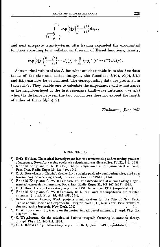
THEORY OF COUPLED ANTENNAE

1

I 'exp ~ty(]-~)~dsfs,

l~ x'1+---y' Y

and, next integrate term-by-term, after having expanded the exponentialfunction according to a well-known theorem of Bessel functions, namely,

As numerical values of the N-functions are obtainable from the Americantables of the sine and cosine integrals, the functions H(O), 1((0), H(l)and K(l) can now be determined. The corresponding data are presented intables U-V. They enable one to calculate the impedances and admittancesin the neighbourhood of the first resonance (half-wave antenna, x ~ 1[12)when the distance between the two conductors does not exceed the lengthof either of them (dil ~ 2).

Eindhoven, June 1947

REFERENCES

1) Erik Hallén, Theoretical investigations into the transmitting and receiving qualitiesof antennae, Nova Acta regiae societatis scientiarum upsaliensis, Scr. IV, 11,1-44,1938.

2) Ronold King and F. G. Blake, The self-impedance of a symmetrical antenna,Proc. Inst. Radio Engrs 30, 335-349, 1942.

3) C. J. Bouwkamp, Hallën's theory for a straight perfectly conducting wire, used as atransmitting or receiving aerial; Physica, 's-Crav. 9, 609-631, 1942.

4) Ronold King and C. W. Harrison, Jr, The distribution of current along a sY,m-metrical center-driven antenna, Proc. Inst. Radio Engrs 31, 548-567 (697), 1943.

5), C. J. Bouwkamp, Laberatory report nr 1731, November 1942 (unpublishedjv6) Ronold King and C. W. Harrison, Jr, Mutual and self-impedance for coupled

antennas, J. appl. Phys. 15, 481-495, 1944.7) Federal Works Agency, Work projects administration for the City of New York,

Tables of sine, cosine and exponential integrals, vols I, Il, New York, 1940;.'rables of,sine and cosine integrals, New York, 1942.

8), C. W. Harrison, Jr, A note on the mutual impedance of antennas, J. appl. Phys.1.4,306-309, 1943. .

0) • C. ~ ein b aum, On the solution of definite integrals' occurring in antenna theory,J.app[ Phys. 15, 840-841, 1944. ' . . . : .

10) C. 'J. Böuwkamp, Laberatory report nr 1693, Jun~ 194.2 (unpublished). ,.

223

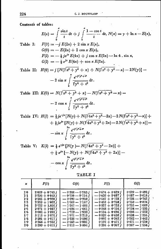
224 C, J, BOUWKAID'

Contents of tables:x x .

f sin t f 1- cos tE(x)= -t-dt+j t dt,N(x)=y+Inx-E(x),o 0

Table I: F(O) = -j E(2x) + 2 sin x E(x),G(O) = - E(2x) + 2 cos x E(x),F(l) = - i jej" E(4x) + j cosx E(2x) -In 4 . sinx,G(l) =- i ej" E(4x) + cos x E(2x).

Table H: H(O) = j [N(Yx2 + y2 + x) + N(Yx2 + y2 - x) - 2N(y)]-'x _jJ'yi+-"

-2 sin x f e dt.o yy2 + t2

Table HI: K(O) = N(Yx2 + y2 + x) -N(Yx2 + ya_x)-" -jl'y'+"

- 2 cos x f ; dt.ly2 + t2

• 0

Table IV: H(l) = tje-jX[N(y) + N(Y4x2+y2_2x)-2N(Y~-x)]+

+ tjejx [N(y) +N(Y4x2+y2+ 2x)-2N(1x2+y2+x)]-2" -jJ'yq: li

-sinx f ~ dt.o ly2 + t2

Table V: K(l) = i e-jx [N(y )- N(Y 4x2 + ya - 2x)] ++ i ejx [- N(y) + N(Y4x2 + y2 + 2x)]-

2:c -jJ'y'+ I"

- cosx r ; dt.o y2+t2

TABLE I

x F(O) G(O) F(l) G(l)

1'0 2'009 + 0'745 i - 0'588 - 0'583 i - 0'674 + 0'629 i 0'629 - O'493i1'1 2'200 + 0'843 i - 0'730 - 0'754 i - 0'620 + 0'687 i 0'687 - 0'616 j1'2 2'385 + 0'930 j - 0'890 - 0'950 j -0'547 + O'728i 0'728 - 0'745 i1'3 2'559 + l'002i -1'069 -1'167 i - 0'458 + O'750j 0'750 - 0'878 j1'4 2'722 + 1.056 j - 1'267 - 1'405 i - 0'357 + 0'753 j 0'753 - 1'009 i1'5 2'871 + 1'087 j -l'484-1'661j -0'248 + O'734j 0'734 - 1'135 i1'6 ·3'002 + l'092j -1'719 -l'933i - 0'134 + 0'696 i 0'696 - 1'252 i1'7 3'113 + 1'070 i - 1'971 - 2'215 j - 0'020 + 0'638 j 0'638 - 1'355 i1'8 3'201 + 1'017 i - 2'238 - 2'506 j 0'092 + O'562j 0'562-I'442i1'9 3'264 + 0'932 i - 2'663 - 2'801j 0'192 + O'471j O'471-1'510i2'0 3'299 + 0'815 i - 2'810 - 3'094 j 0'296 + 0'367 j 0'367 - 1'556 j

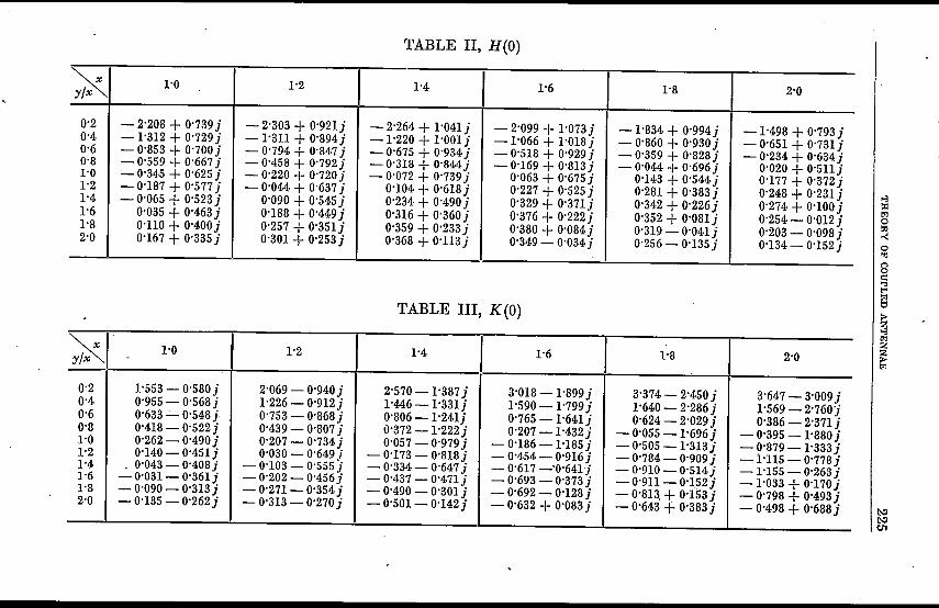
TABLE rr, H(O)

~1'0 1'2 1'4 1'6 1'8 2'0,

0'2 - 2'208 + 0'739 i - 2'303 + 0'921 i - 2'264 + 1'041i - 2'099 + 1'073 i -1'834 + 0'994i - 1'498 + 0'793 i0'4 -1'312 + 0'729 i -1'311 + 0'894i -1'220 + r-ooi , -1'066 + l'018i - 0'860 + 0'930 i - 0'651 + 0'731i0'6 - 0'853 + 0'700 i - 0'794 + 0'847 i - 0'675 + 0'934 i - 0'518 + 0'929 i - 0'359 + 0'828 i - 0'234 + 0'634 j0'8 - 0'559 + 0'667 j - 0'458 + 0'792j - 0'318 + 0'844 j - 0'169 + 0'813 j - 0'044 + 0'696 j 0'020 + 0'511j1'0 - 0'34.5+ 0'625 j - 0'220 + 0'720 j - 0'072 + 0'739 j 0'063 + 0'675 i 0'143 + 0'544j 0'177 + 0'372i1'2 - 0'187 + 0'577 i - 0'044 + 0'637 i 0'104 + 0'618i 0'227 + 0'525 i 0'281 + 0'383 i 0'248 + 0'231 i '":l1'4 - 0'065 + 0'523 i 0'090 + 0'54·5i 0'234 + 0'490 i 0'329 + 0'371} 0'342 + 0'226 i 0'274 + 0'100 i =l'l1'6 0'035 + 0'463 i 0'188 + 0'449 i 0'316 + 0'360 j 0'376 + 0'222i 0'352 + 0'081i 0'254 - 0'012 i 01'8 0'110 + 0'400i 0'257 + 0'351i 0'359 + 0'233 j 0'380 + 0'084j 0'319 - 0'041j 0'203 - 0'098 j !:d-<2'0 0'167 + 0'335 j 0'301 + 0'253i 0'368 + 0'113 j 0'349 - 0'034 j 0'256 - 0'135 i 0'134 - 0'152 i 0"ln0c:1."t"'l'lt:ITABLE Ill, K (0)~ -'":l

I Il'l

~1'0 1'2 1'4 1'6 1'8 2'0 ~

l'l

0'2 1'553 - 0'580 i 2'069 - 0'940 i 2'570 -1'387 i 3'018 - 1'899 i 3'374 - 2"450i 3'647 - 3'009 i0'4 0'955 ~ 0'568 j 1'226 - 0'912j 1'446-1'331i 1'590 -1'799 i 1'640 - 2'286 j 1'569 - 2'760]0'6 0'633 - 0'548 i 0'753 - 0'868 j 0'806-1'241j 0'765-1'641i 0'624 - 2'029 i 0'386 - 2'371 i0'8 0'418 - 0'522i 0'439 - 0'807 j 0'372-1'222j 0'207 - 1'432 j - 0'055 - 1'696 i - 0'395 -1'880 i1'0 0'262 - 0'4·90j 0'207 - 0'734j 0'057 - 0'979 i - 0'186 -l'185i - 0'505 - 1'313 i -0'879-1'333j1'2 0'14·0- 0'451j 0'030 - 0'649 i - 0'173 - 0'818 j - 0'454 - 0'916 i - 0'784 - 0'909 j -1'115 - 0'778 i1'4 . 0'043 - 0'408 j - 0'103 - 0'555 J - 0'334 - 0'647 j - 0'617 -'0'641j - 0'910 - 0'514j -1'155 - 0'263j1'6 - 0'031 - 0'361 j - 0'202 - 0'456 j - 0'437 - O'471j - 0'693 - 0'373 j - 0'911- O'152i -1'033 + 0'170j1'8 ~ 0'090 - 0'313 i - 0'271 - 0'354 i - 0'490 - 0'301i - 0'692 - 0'128 i - O'81~+ 0'153 i - 0'798 + 0'493 i2'0 - 0'135 - 0'262i - 0'313 - 0'270 i - 0'501- 0'142i - 0'632 + 0'083 i - 0'643 + 0'383 j - 0'498 + 0'688 j ~~til

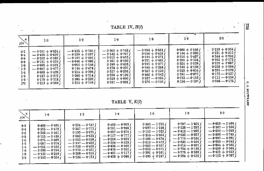
TABLE IV, H(l)

~I -]:0 1-2 1"4 1-6 1-8 2:0

0-2 - 0-551 + 0-624 j - 0:433 + 0-720 j - 0-266 + 0-742j - 0-084 + 0:681 j 0-086 + 0-546 j 0-219 + 0-354j

0-4 - 0-426 + 0-609 j - 0-299 + 0-697 j - 0-14·2+ 0-707 j 0-016 + 0-638j 0-144 + 0-500 i. 0-221 + 0-312}

0-6 - 9-302 + 0-589 j - 0-167 + 0-660j - 0-015 + 0-652j 0-124 + 0-571j 0-216 + 0-427 j 0-244 + 0-250j

0-8 ; - 0-191 + 0-559 j - 0-048 + 0-608 j 0-101 + 0-580 j 0-221 + 0-482j 0-281 + 0-334 j 0-265 + 0-172i.

1-0 - 0-093 + 0-521 j 0-056 + 0-546 j 0-199 + 0-493j 0-297 + 0-377 j 0-324 + 0-229 j 0-272 + 0-087 j.. 1-2 - 0-007 + 0-477 j 0-144.+ 0-474j 0-274 + 0-397 j 0-346 + 0-264 j 0-340 + 0-120 i 0-258 + 0-004 j

1-4 0-065 + 0-4.28j 0-214 + 0-396 j 0-327 + 0-293 j 0-367 + 0-150 j 0-328 + 0-016 j 0-225 - 0-070 j

1-6 0-127 + 0-375 j 0-266 + 0-314.j 0-358 + 0-189 j 0-360 + 0-042j 0-291 - 0-077 j 0-172 - 0-127 j

1-8 - 0-179 + 0-318j 0-301 + 0-232j 0-359 + 0-090 j 0-327 - 0-055 j 0-233 - 0-153 j 0-111- 0-164 j

!!'·O 0-213 + 0-260 j 0-316 + 0-149 j 0-337 - 0-001 j 0-276 - 0-135 j 0-156 - 0-197 j 0-046 - 0-175 j

TABLE V, K(l)

~I 1-0 1-2 1-4 1-6 1-8 2-0

0-2 0-480 - 0-490 j 0-524 - 0-737 j 0-493 - 0-993 j 0-383 -1-225j 0-207 -1"401j - 0-018 -1-499 j

0-4 0-355 - 0-479 j 0-347 - 0-713 j 0-261 - 0-949 j 0-097--1-148j - 0-128 -1-282j - 0-387 - 1-330 j

0-6 0-248 - 0-461 j 0-193 - 0-675 j 0-057 - 0-874 j - 0-150 -1-025j - 0-412 - 1-095 j - 0-690 -1-069 j

0-8 0-155 - 0-438 j 0-060 - 0-623 j - 0-117 - 0-777 j - 0-354 - 0-864 j - 0-632 - 0-857 j - 0-898 - 0-745 j

1-0 0-075 - 0-409 j - 0-053 - 0-558 j - 0-258 - 0-659 j - 0-508 - 0-676 j - 0-774 - 0-586 j - 0-997 - 0-391 j

1-2 0-007 - 0-374 j - 0-147 - 0-485j - 0-364 - 0-529 j - 0-610 - 0-472j - 0-833 - 0-305 j - 0-983 - 0-043 jI-Ij, - 0-051 - 0-335 j - 0-220 - 0-405 j - 0-436 - 0-390 j - 0-660 - 0-267 j - 0-814 - 0-037 j - 0-864 + 0-265 j1-6 - 0-098 - 0-294.j - 0-273 - 0-321 j - 0-476 - 0-252 j - 0-650 - 0-071 j - 0-724 + 0-198 j - 0-669 + 0-503 j

1-8 - 0-135 - 0-249 j - 0-308 - 0-235 j - 0-481- 0-117 j - 0-591 + 0-101 j - 0-578 + 0-388 j - 0-421 + 0-653 j

2-0 - 0-163 - 0-204} - 0-324 - 0-151j - 0-458 + 0-006 j - 0-4.96 -t 0-247 j - 0-394 + 0-510 j - 0-152 + 0-707 j.

.. . .. .

~~0\

p~tij

~~