Embed Size (px)
Citation preview
On The Transmission of Global Shocks to Latin AmericaBefore and After China’s Emergence in the World
Economy∗
Ambrogio Cesa-BianchiInter-American Development Bank
M. Hashem PesaranUniversity of Cambridge
Alessandro RebucciInter-American Development Bank
Cesar E. TamayoInter-American Development Bank
TengTeng XuUniversity of Cambridge
First Draft: June 4, 2010Preliminary and Incomplete.
Abstract
External shocks are very important for Latin America’s economic performance as the re-cent global crisis vividly illustrated. At the same time, the global economy has undergoneprofound structural changes over the past three decades. This paper investigates howchanged trade linkages between China, Latin America, and the rest of the world maybe affecting the transmission of global shocks to Latin America. Preliminary evidencebased on a GVAR model estimated with quarterly data from 1979(1) to 2008(2) for allmajor advanced and emerging economies of the world show that the impact of a globalGDP shock on the typical Latin American economy may have halved between 1995-97and 2005-07, due to the increased weight of China international trade in total trade forLatin America, the United States, and the euro area. Over the same period, we do notfind evidence of increased impact of regional GDP shocks in Latin America or emergingAsia excluding China as the popular decoupling hypothesis would imply. These resultssuggest that one reason why these regions are doing so well in the aftermath of the globalcrisis is sheer ”good luck”.
Keywords: China, Globalization, Trade Linkages, GVAR, Business Cycle.
JEL Classification Numbers:
∗The views expressed in this paper are exclusively those of the authors and not those of the IDB or itsExecutive Board.
1
1 Introduction
External factors are very important for Latin America’s economic performance as the impact
of the global crisis on the region has vividly illustrated.1 But the world economy has undergone
profound structural changes over the past two-three decades because of globalization and the
emergence of China, India, and other large developing economies (including Mexico and Brazil
in Latin America) as global economic players. As a result, the importance and the transmission
mechanisms of external shocks to Latin American economies may now have changed.
This paper focuses on the emergence of China as a global force in the world economy and
investigates how changed trade patterns between China and the rest of the world may have
affected the impact and transmission of external shocks to Latin America. We focus on China
because, as we shall see, its trade linkages with the rest of the world are those that have
undergone the most dramatic change over the period we consider. Specifically, we address
the following questions: Is the importance of external shocks for the typical Latin American
economy stable over time? What is the role of China and the rest of emerging Asia in the
transmission of global shocks to Latin America? Are shocks originating from the US and the
euro area, which remain the largest trading partners, transmitted differently than shocks from
China and the rest of Asia? Are regional (i.e., LAC shocks) becoming more important over
time for LAC?
To conduct the empirical analysis we use a variant of the global vector autoregression
model (GVAR) originally presented by Pesaran, Schuermann, and Weiner (2004) and further
developed by Dees, di Mauro, Pesaran, and Smith (2007). The model includes 25 major
advanced and emerging economies and the euro area, covering more than 90 percent of world
GDP, and including five large Latin American economies (Argentina, Brazil, Chile, Mexico,
and Peru). The data set is quarterly, starting in 1979(1), and is updated to 2008(2).
One characteristic of the GVAR model is its remarkable parameter stability. Even for Latin
American economies that have experienced frequent changes in policy regime and other deep
structural changes, standard statistical tests do not identify widespread parameter instability.
We build on this strength of the GVAR, and use a different set of trade weights to construct
counter factual simulations of what would the impact of external shocks and their transmission
mechanisms be under alternative configurations of the trade linkages between China and the
rest of the world.
To address the questions above we thus simulate a given set of external shocks in the GVAR
model using alternative sets of trade weights that capture one important aspect of China’s
changed role in the world economy: its new pattern of trade linkages with the rest of the world.
The focus of our study is on real shocks. In particular, we analyze shocks to global output,
to US output, to euro area output, China output, as well as regional (i.e., Latin American and
1For empirical analyses of the impact of external factors on Latin American’s economic performance see,among many other contributions, Little et al (1993), Hoffmaister and Roldos (1998), Canova (2005), Osterholmand Zettelmeyer (2007), Izquierdo, Romero, and Talvi (2008), and Rebucci (2008).
2
Rest of Emerging Asia) output.
Preliminary empirical results show that the importance of a global GDP shock for the
typical Latin American economy may have halved over time. At the same time, we do not
find evidence that regional shocks have increased their importance over time, contrary to the
popular notion of decoupling.
The rest of the paper is organized as follows. In the next section, we discuss how the trade
linkages between China and the rest of the world, and particularly LAC, have evolved over
time. In Section 3, we describe the GVAR model that we use and we discuss its estimation
based on the updated data set we constructed. Section 4 reports the counter factual simulation
results. Section 5 concludes. Two appendices describe in details the update of the data set and
report a full set of the baseline estimation results for the GVAR model based on 2001-03 trade
weights.
2 The Changing Weight of China in the World Economy
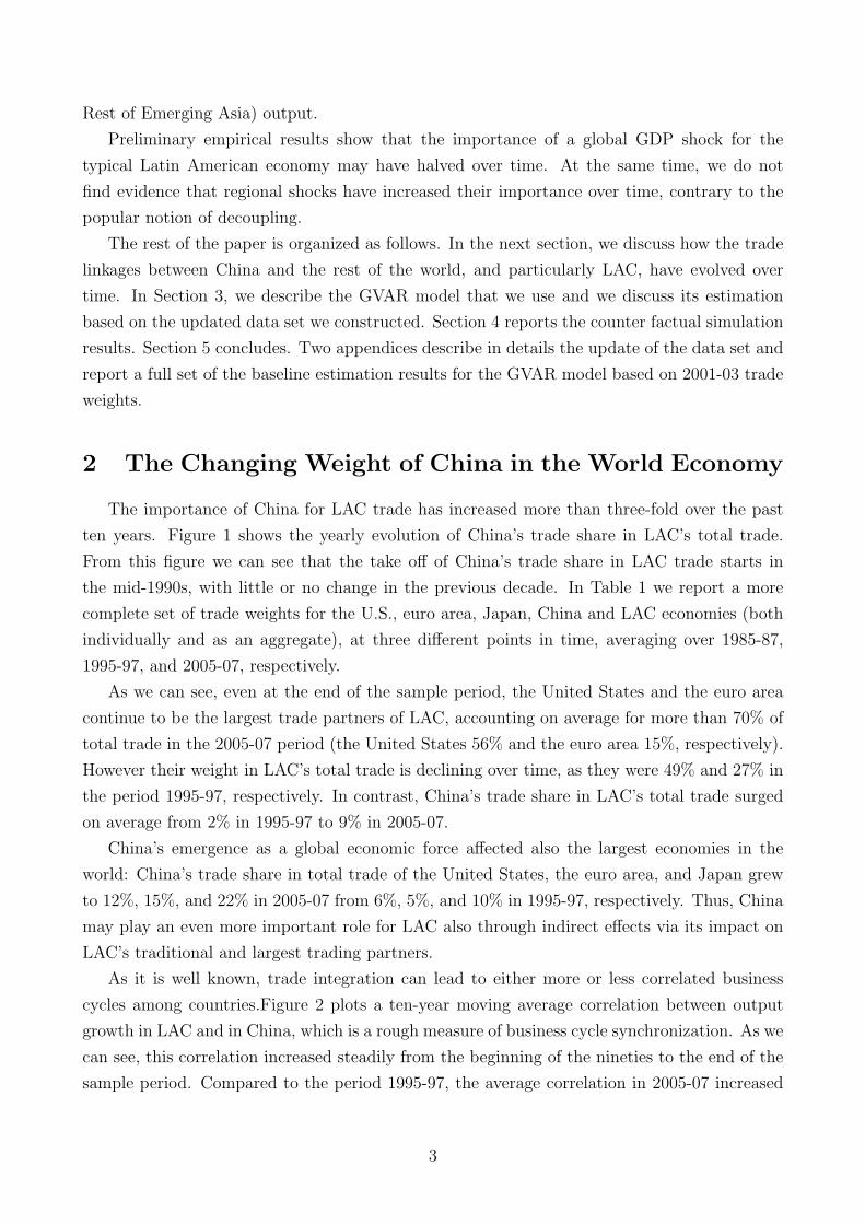
The importance of China for LAC trade has increased more than three-fold over the past
ten years. Figure 1 shows the yearly evolution of China’s trade share in LAC’s total trade.
From this figure we can see that the take off of China’s trade share in LAC trade starts in
the mid-1990s, with little or no change in the previous decade. In Table 1 we report a more
complete set of trade weights for the U.S., euro area, Japan, China and LAC economies (both
individually and as an aggregate), at three different points in time, averaging over 1985-87,
1995-97, and 2005-07, respectively.
As we can see, even at the end of the sample period, the United States and the euro area
continue to be the largest trade partners of LAC, accounting on average for more than 70% of
total trade in the 2005-07 period (the United States 56% and the euro area 15%, respectively).
However their weight in LAC’s total trade is declining over time, as they were 49% and 27% in
the period 1995-97, respectively. In contrast, China’s trade share in LAC’s total trade surged
on average from 2% in 1995-97 to 9% in 2005-07.
China’s emergence as a global economic force affected also the largest economies in the
world: China’s trade share in total trade of the United States, the euro area, and Japan grew
to 12%, 15%, and 22% in 2005-07 from 6%, 5%, and 10% in 1995-97, respectively. Thus, China
may play an even more important role for LAC also through indirect effects via its impact on
LAC’s traditional and largest trading partners.
As it is well known, trade integration can lead to either more or less correlated business
cycles among countries.Figure 2 plots a ten-year moving average correlation between output
growth in LAC and in China, which is a rough measure of business cycle synchronization. As we
can see, this correlation increased steadily from the beginning of the nineties to the end of the
sample period. Compared to the period 1995-97, the average correlation in 2005-07 increased
3
by 84%, from 0,27 to 0,49.2 All countries considered display a pattern similar to the regional
one except Mexico, which goes from negative to about zero , and Brazil, which experiences a
650% increase of compared to the 1995-97 period.3
In sum, growing trade linkages between China and the rest of the world (including LAC) as
documented above are clearly associated with more synchronized business cycles between LAC
and China. And as we shall see below, this association can be interpreted as a causation.
3 The GVAR Model
The GVAR modelling strategy consists of three main steps. First, each country is modeled
individually as a small open economy by estimating a country-specific vector error-correction
model in which domestic macroeconomic variables (xit) are related to country-specific foreign
variables (x∗it). Global variables (dt), that are common among all countries such as the oil price,
are also included in each of the country-specific model and assumed to be weakly exogenous.
Second, a restricted reduced-form global model is built stacking the estimated country-specific
models and connecting them through a matrix of trade linkages (W). Third and finally, tak-
ing into account the possibility that the error terms of this restricted reduced form model
are correlated contemporaneously, Generalized Impulse Response Functions (GIRFs) and the
Generalized Forecast Error Variance Decompositions (GFEVDs)—developed in Koop, Pesaran,
and Potter (1996) and Pesaran and Shin (1998)—are computed to analyze the transmission of
shocks and their historical importance.
The foreign country-specific variables, x∗it, play a central role in the GVAR. They are con-
structed as trade-weighted averages of the corresponding variables in all the other countries in
the GVAR model and statistically they are assumed to be weakly exogenous. Thus:
x∗it =
N∑j=0
ωijxjt, (1)
where ωij is the trade weight of country j in the model for country i, with ωii = 0. Note also
that, although the number of countries does not need to be large for the GVAR to work, when
it is small, then, at least for one country this weak exogeneity assumption cannot be satisfied.
It is only when the number of countries tends to infinity and all countries are relatively small
that we can have a symmetric treatment of all of them in the GVAR. For this reason, as we
shall see below, we treat the united United States differently in GVAR.
Consider N +1 countries in the global economy, indexed by i = 0, 1, 2, ...N . In the first step,
2Notice that output growth rate in LAC is computed based on a weighted average of LAC countries outputusing PPP-GDP weights averaged over the period 2001-03. (Source PWT 6.1.)
3This is consistent with the evidence (up to end-2004) reported by Calderon (2008). Interestingly, Calderon(2008) finds that such an increased output correlation with China is better explained by China’s share of totaltrade of third parties and its large demand share in commodity markets rather than direct bilateral tradelinkages between LAC and China.
4
each country i is represented by a vector autoregressive model for the xit augmented by weakly
exogenous variables. Specifically a VARX*(pi,qi) model, in which the (ki × 1) country-specific
domestic variables are related to the (k∗i ×1) foreign-specific and (md×1) global variables, plus
constant and a deterministic time trend is set up for each country i:
Φi(L, pi)xit = ai0 + ai1t + Υi(L, qi)dt + Λi(L, qi)x∗it + uit, (2)
for i = 0, 1, ..., N and t = 1, ..., T . Notice that: Φi(L, pi) = I −∑pi
i=1 ΦiLi is the matrix lag
polynomial of the coefficients associated to the xit; ai0 is a ki × 1 vector of fixed intercepts; ai1
is a ki × 1 vector of coefficients of the deterministic time trend; Υi(L, qi) =∑qi
i=0 ΥiLi is the
matrix lag polynomial the coefficients associated to the dt; Λi(L, qi) =∑qi
i=0 ΛiLi is the matrix
lag polynomial of the coefficients associated to the x∗it; uit is a ki × 1 vector of country-specific
shocks, which we assume serially uncorrelated, with zero mean, and nonsingular covariance
matrix, uit ∼ i.i.d.(0,Σii). Notice also that for estimation purposes Φi(L, pi), Υi(L, qi), and
Λi(L, qi) can be treated as unrestricted and can differ across countries.
The error correction form of equation (2) may be written as
∆xit = ci0 − αiβ′i[ζ i,t−1 − γi(t− 1)] (3)
+ Υi0∆dt + Λi0∆x∗it + Υi1∆dt−1 + Γi∆zi,t−1 + uit,
where zit = (x′it,x
′∗it)
′, ζ i,t−1 = (z′i,t−1,d′t−1)
′, αi is a ki × ri matrix of rank ri and β is a
(ki + k∗i + md)× ri matrix of rank ri. By partitioning βi as βi = (β′ix, β
′ix∗ , β′
id)′ conformable to
ζ i,t = (x′it,x
′∗it,d
′t)′ the ri error correction terms implicit in equation 3 can now be written as:
β′(ζ it − γit) = β′ixxit + β′
ix∗x∗it + β′iddt + (β′
iγi)t,
which clearly allows for the possibility of cointegration both within xit, and between xit and
x∗it and consequently across xit and xjt for i 6= j. Interdependence among countries in the
GVAR model can thus arises through the interaction of xit with x∗it, through the dependence
of xit on global variables dt, and through the contemporaneous interdependence of shocks in
country i on the shocks in country j, as described by the cross-country covariances, Σij, where
Σij = Cov(uit,ujt) = E(uitu′jt) for i 6= j.
The above country-specific vector error-correction models (VECMXs) can now be consis-
tently estimated, treating dt and x∗it as weakly exogenous with respect to the long-run parame-
ters of the conditional model of equation 3. In practice, the weak exogeneity assumption allows
to consider each country as a small open economy with respect to the rest of the world and,
therefore, it allows a country-by-country estimation.
In the second step, once the individual country models are estimated, all the k =∑N
i=0 ki
endogenous variables of the global economy are stacked together in the k × 1 vector xt =
5
(x′0t,x
′1t, ...,x
′Nt)
′. To do this, first we stack domestic and the foreign country-specific variables
in the vector
zit = [x′it,x
′∗it]
′
and we re-write equation 2 as
Ai(L, pi, qi)zit = ϕit, i = 0, 1, 2, ..., N (4)
where
Ai(L, pi, qi) = [Φi(L, pi),−Λi(L, qi)],
ϕit = ai0 + ai1t + Υi(L, qi)dt + uit,
Let p = max(p0, p1, ..., pN , q0, q1, ..., qN) and construct Ai(L, p) from Ai(L, pi, qi) by augmenting
the p− pi or p− qi additional terms in powers of L by zeros.
Note now that, given 1, we can write zit as:
zit = Wixt, i = 0, 1, 2, ..., N, (5)
where Wi is a (ki + k∗i )× k matrix defined by the country specific trade weights, ωij. So 4 can
be written as
Ai(L, p)Wixt = ϕit, i = 0, 1, 2, ..., N.
And by stacking together the country specific models, we have:
G(L, p)xt = ϕt, (6)
where
G(L, p) =
A0(L, p)W0
A1(L, p)W1
...
AN(L, p)WN
, and ϕt =
ϕ0t
ϕ1t...
ϕN t
.
Assuming then that G is non-singular, the GVAR(p) (6) can be solved recursively and used
for forecasting or generalized impulse response and variance decomposition analysis in the usual
manner.
6
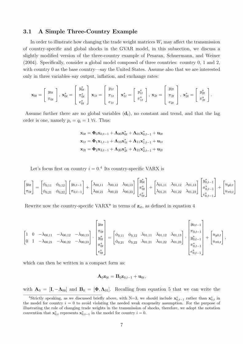
3.1 A Simple Three-Country Example
In order to illustrate how changing the trade weight matrices Wi may affect the transmission
of country-specific and global shocks in the GVAR model, in this subsection, we discuss a
slightly modified version of the three-country example of Pesaran, Schuermann, and Weiner
(2004). Specifically, consider a global model composed of three countries: country 0, 1 and 2,
with country 0 as the base country—say the United States. Assume also that we are interested
only in three variables–say output, inflation, and exchange rates:
x0t =
[y0t
π0t
], x∗0t =
y∗0t
π∗0t
e∗0t
x1t =
y1t
π1t
e1t
x∗1t =
[y∗1t
π∗1t
], x2t =
y2t
π2t
e2t
, x∗2t =
[y∗2t
π∗2t
].
Assume further there are no global variables (dt), no constant and trend, and that the lag
order is one, namely pi = qi = 1 ∀i. Thus:
x0t = Φ0x0,t−1 + Λ00x∗0t + Λ01x∗0,t−1 + u0t
x1t = Φ1x1,t−1 + Λ10x∗1t + Λ11x∗1,t−1 + u1t
x2t = Φ2x2,t−1 + Λ20x∗2t + Λ21x∗2,t−1 + u2t
Let’s focus first on country i = 0.4 Its country-specific VARX is
[y0t
π0t
]=
[φ0,11 φ0,12
φ0,21 φ0,22
] [y0,t−1
π0,t−1
]+
[λ00,11 λ00,12 λ00,13
λ00,21 λ00,22 λ00,23
] y∗0t
π∗0t
e∗0t
+
[λ01,11 λ01,12 λ01,13
λ01,21 λ01,22 λ01,23
] y∗0,t−1
π∗0,t−1
e∗0,t−1
+
[uy0,t
uπ0,t
]
Rewrite now the country-specific VARX* in terms of zit, as defined in equation 4
[1 0 −λ00,11 −λ00,12 −λ00,13
0 1 −λ00,21 −λ00,22 −λ00,23
]·
y0t
π0t
y∗0t
π∗0t
e∗0t
=
[φ0,11 φ0,12 λ01,11 λ01,12 λ01,13
φ0,21 φ0,22 λ01,21 λ01,22 λ01,23
]·
y0,t−1
π0,t−1
y∗0,t−1
π∗0,t−1
e∗0,t−1
+
[uy0,t
uπ0,t
],
which can then be written in a compact form as:
A0z0t = B0z0,t−1 + u0t,
with A0 = [I,−Λ00] and B0 = [Φ,Λ01]. Recalling from equation 5 that we can write the
4Strictly speaking, as we discussed briefly above, with N=3, we should include x∗0,t−1 rather than x∗0,t inthe model for country i = 0 to avoid violating the needed weak exogeneity assumption. For the purpose ofillustrating the role of changing trade weights in the transmission of shocks, therefore, we adopt the notationconvention that x∗0,t represents x∗0,t−1 in the model for country i = 0.
7
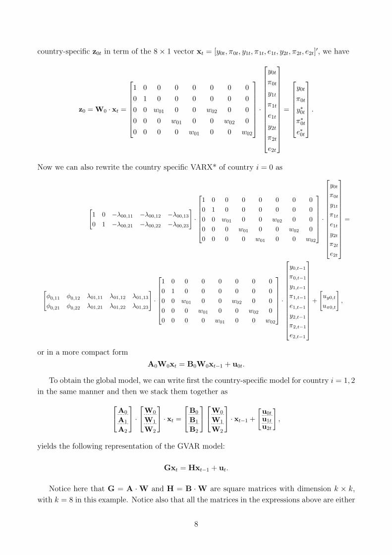
country-specific z0t in term of the 8× 1 vector xt = [y0t, π0t, y1t, π1t, e1t, y2t, π2t, e2t]′, we have
z0 = W0 · xt =
1 0 0 0 0 0 0 0
0 1 0 0 0 0 0 0
0 0 w01 0 0 w02 0 0
0 0 0 w01 0 0 w02 0
0 0 0 0 w01 0 0 w02
·
y0t
π0t
y1t
π1t
e1t
y2t
π2t
e2t
=
y0t
π0t
y∗0t
π∗0t
e∗0t
.
Now we can also rewrite the country specific VARX* of country i = 0 as
[1 0 −λ00,11 −λ00,12 −λ00,13
0 1 −λ00,21 −λ00,22 −λ00,23
]·
1 0 0 0 0 0 0 00 1 0 0 0 0 0 00 0 w01 0 0 w02 0 00 0 0 w01 0 0 w02 00 0 0 0 w01 0 0 w02
·
y0t
π0t
y1t
π1t
e1t
y2t
π2t
e2t
=
[φ0,11 φ0,12 λ01,11 λ01,12 λ01,13
φ0,21 φ0,22 λ01,21 λ01,22 λ01,23
]·
1 0 0 0 0 0 0 00 1 0 0 0 0 0 00 0 w01 0 0 w02 0 00 0 0 w01 0 0 w02 00 0 0 0 w01 0 0 w02
·
y0,t−1
π0,t−1
y1,t−1
π1,t−1
e1,t−1
y2,t−1
π2,t−1
e2,t−1
+
[uy0,t
uπ0,t
],
or in a more compact form
A0W0xt = B0W0xt−1 + u0t.
To obtain the global model, we can write first the country-specific model for country i = 1, 2
in the same manner and then we stack them together asA0
A1
A2
·W0
W1
W2
· xt =
B0
B1
B2
W0
W1
W2
· xt−1 +
[u0tu1tu2t
],
yields the following representation of the GVAR model:
Gxt = Hxt−1 + ut.
Notice here that G = A ·W and H = B ·W are square matrices with dimension k × k,
with k = 8 in this example. Notice also that all the matrices in the expressions above are either
8
known or estimated. Specifically, through the estimation of the country-specific VECMXs, we
pin down the matrices Φ0, Λ00, and Λ01 and, therefore, we can construct A0, B0. The vector of
constants, the coefficients on the time trend, and the estimated error terms are also estimated
within the VECMXs. In contrast, the matrix of trade linkages W0, is derived directly from
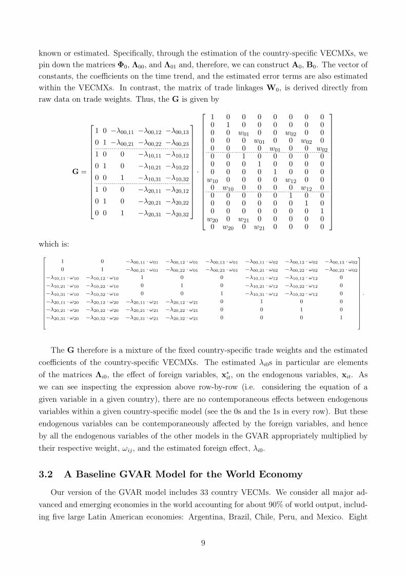
raw data on trade weights. Thus, the G is given by
G =
1 0 −λ00,11 −λ00,12 −λ00,13
0 1 −λ00,21 −λ00,22 −λ00,23
1 0 0 −λ10,11 −λ10,12
0 1 0 −λ10,21 −λ10,22
0 0 1 −λ10,31 −λ10,32
1 0 0 −λ20,11 −λ20,12
0 1 0 −λ20,21 −λ20,22
0 0 1 −λ20,31 −λ20,32
·
1 0 0 0 0 0 0 00 1 0 0 0 0 0 00 0 w01 0 0 w02 0 00 0 0 w01 0 0 w02 00 0 0 0 w01 0 0 w020 0 1 0 0 0 0 00 0 0 1 0 0 0 00 0 0 0 1 0 0 0
w10 0 0 0 0 w12 0 00 w10 0 0 0 0 w12 00 0 0 0 0 1 0 00 0 0 0 0 0 1 00 0 0 0 0 0 0 1
w20 0 w21 0 0 0 0 00 w20 0 w21 0 0 0 0
which is:
1 0 −λ00,11 · ω01 −λ00,12 · ω01 −λ00,13 · ω01 −λ00,11 · ω02 −λ00,12 · ω02 −λ00,13 · ω02
0 1 −λ00,21 · ω01 −λ00,22 · ω01 −λ00,23 · ω01 −λ00,21 · ω02 −λ00,22 · ω02 −λ00,23 · ω02
−λ10,11 · ω10 −λ10,12 · ω10 1 0 0 −λ10,11 · ω12 −λ10,12 · ω12 0
−λ10,21 · ω10 −λ10,22 · ω10 0 1 0 −λ10,21 · ω12 −λ10,22 · ω12 0
−λ10,31 · ω10 −λ10,32 · ω10 0 0 1 −λ10,31 · ω12 −λ10,32 · ω12 0
−λ20,11 · ω20 −λ20,12 · ω20 −λ20,11 · ω21 −λ20,12 · ω21 0 1 0 0
−λ20,21 · ω20 −λ20,22 · ω20 −λ20,21 · ω21 −λ20,22 · ω21 0 0 1 0
−λ20,31 · ω20 −λ20,32 · ω20 −λ20,31 · ω21 −λ20,32 · ω21 0 0 0 1
.
The G therefore is a mixture of the fixed country-specific trade weights and the estimated
coefficients of the country-specific VECMXs. The estimated λi0s in particular are elements
of the matrices Λi0, the effect of foreign variables, x∗it, on the endogenous variables, xit. As
we can see inspecting the expression above row-by-row (i.e. considering the equation of a
given variable in a given country), there are no contemporaneous effects between endogenous
variables within a given country-specific model (see the 0s and the 1s in every row). But these
endogenous variables can be contemporaneously affected by the foreign variables, and hence
by all the endogenous variables of the other models in the GVAR appropriately multiplied by
their respective weight, ωij, and the estimated foreign effect, λi0.
3.2 A Baseline GVAR Model for the World Economy
Our version of the GVAR model includes 33 country VECMs. We consider all major ad-
vanced and emerging economies in the world accounting for about 90% of world output, includ-
ing five large Latin American economies: Argentina, Brazil, Chile, Peru, and Mexico. Eight
9
countries belong to the euro area and are therefore analyzed as a group.5 The remaining 25
countries are modeled individually. Thus, the version of the GVAR model that we use contains
26 countries.
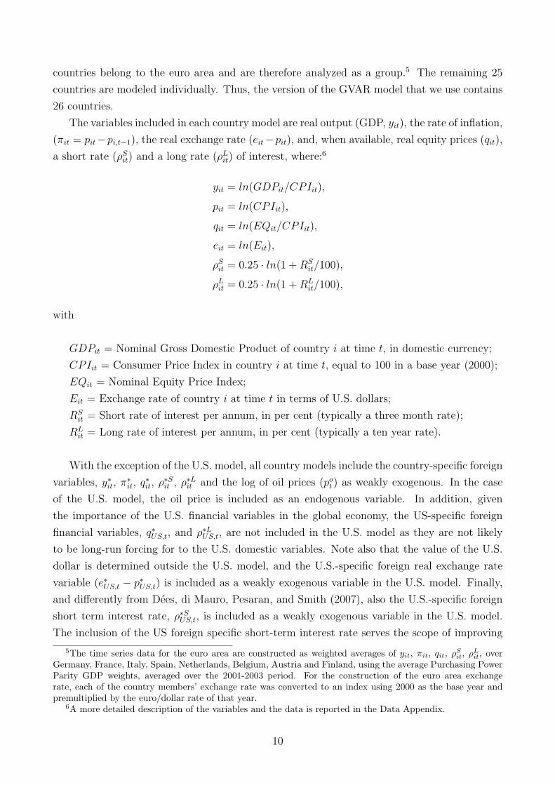
The variables included in each country model are real output (GDP, yit), the rate of inflation,
(πit = pit−pi,t−1), the real exchange rate (eit−pit), and, when available, real equity prices (qit),
a short rate (ρSit) and a long rate (ρL
it) of interest, where:6
yit = ln(GDPit/CPIit),
pit = ln(CPIit),
qit = ln(EQit/CPIit),
eit = ln(Eit),
ρSit = 0.25 · ln(1 + RS
it/100),
ρLit = 0.25 · ln(1 + RL
it/100),
with
GDPit = Nominal Gross Domestic Product of country i at time t, in domestic currency;
CPIit = Consumer Price Index in country i at time t, equal to 100 in a base year (2000);
EQit = Nominal Equity Price Index;
Eit = Exchange rate of country i at time t in terms of U.S. dollars;
RSit = Short rate of interest per annum, in per cent (typically a three month rate);
RLit = Long rate of interest per annum, in per cent (typically a ten year rate).
With the exception of the U.S. model, all country models include the country-specific foreign
variables, y∗it, π∗it, q∗it, ρ∗Sit , ρ∗Lit and the log of oil prices (po
t ) as weakly exogenous. In the case
of the U.S. model, the oil price is included as an endogenous variable. In addition, given
the importance of the U.S. financial variables in the global economy, the US-specific foreign
financial variables, q∗US,t, and ρ∗LUS,t, are not included in the U.S. model as they are not likely
to be long-run forcing for to the U.S. domestic variables. Note also that the value of the U.S.
dollar is determined outside the U.S. model, and the U.S.-specific foreign real exchange rate
variable (e∗US,t − p∗US,t) is included as a weakly exogenous variable in the U.S. model. Finally,
and differently from Dees, di Mauro, Pesaran, and Smith (2007), also the U.S.-specific foreign
short term interest rate, ρ∗SUS,t, is included as a weakly exogenous variable in the U.S. model.
The inclusion of the US foreign specific short-term interest rate serves the scope of improving
5The time series data for the euro area are constructed as weighted averages of yit, πit, qit, ρSit, ρL
it, overGermany, France, Italy, Spain, Netherlands, Belgium, Austria and Finland, using the average Purchasing PowerParity GDP weights, averaged over the 2001-2003 period. For the construction of the euro area exchangerate, each of the country members’ exchange rate was converted to an index using 2000 as the base year andpremultiplied by the euro/dollar rate of that year.
6A more detailed description of the variables and the data is reported in the Data Appendix.
10
the weak exogeneity tests for US specific foreign inflation and exchange rate.7
In the baseline model specification, the country-specific foreign variables, y∗it, π∗it, q∗it, ρ∗Sit ,
and ρ∗Lit are constructed using fixed trade weights based on the average trade flows over the
three-year period 2001-2003, as in equation 1.8
Detailed empirical evidence on the statistical assumptions made to specify the GVAR model
is reported in the Baseline Model Appendix, together with a description of the impact multi-
pliers and pair-wise correlations for all variables and countries included in the model.9 This
includes evidence on the degree of integration of all individual time series, the lag-length an
the cointegration rank for all country models, as well as test statistics on the weak exogeneity
assumptions made. Because of the importance of parameter stability for the counterfactual
simulation exercise that we conduct in the paper, however, evidence on parameter stability is
discussed here.
The possibility of structural breaks is likely to be particularly acute in the case of Latin
America which was subject to significant political, social and structural reforms. However, the
GVAR can readily accommodate co-breaking, implying that the VECMX models that underlie
the GVAR might be more robust to the possibility of structural breaks as compared to reduced
form single equation models. In any case, we perform formal stability tests following Dees,
di Mauro, Pesaran, and Smith (2007) and consider tests that are based on the residuals of the
individual equations of the country-specific error correction models.10
Among the tests included in our analysis are Ploberger and Kramer’s (1992) maximal OLS
cumulative sum (CUSUM) statistic, denoted by PKsup and its mean square variant PKmsq.
The PKsup statistic is similar to the CUSUM test suggested by Brown, Durbin and Evans
(1975), although the latter is based on recursive rather than OLS residuals. Also considered
are tests for parameter constancy against non-stationary alternatives proposed by Nyblom
(1989), denoted by N, as well as sequential Wald type tests of a one-time structural change at
an unknown change point. The latter include the Wald form of Quandt’s (1960) likelihood ratio
statistic (QLR), the mean Wald statistic (MW ) of Hansen (1992) and Andrews and Ploberger
(1994) and the Andrews and Ploberger (1994) Wald statistic based on the exponential average
(APW ). The heteroskedasticity-robust version of the above tests is also presented.
Table 2 summarizes the results of the tests by variable at the 5% significance level. The
critical values of the tests, computed under the null of parameter stability, are computed using
7Under this assumption, the U.S. model passes the test statistics for weak exogeneity more satisfactorily aswe describe in the Baseline Model Appendix table B.8. (Table B.4 summarizes the model specification for allthe countries included in the GVAR.)
8The weight, ωij , representing the trade share of country j in the total trade of country i, is measured inU.S. dollars and Figure B.1 reports the 26 by 26 matrix which links together the the countries in the model.
9A full set of GIRFs for the baseline model is not reported but is available from the authors on request. Thetransmission properties of the baseline model with 2001-03 trade weights are fully consistent with earlier GVARwork based earlier vintages of the GVAR data set.
10It is well known that these residuals only depend on the rank of the cointegrating vectors and do not dependon the way the cointegrating relations are exactly identified. In this way we render the structural stability testsof the short-run coefficients invariant to exact identification of the long run relations
11
the sieve bootstrap samples obtained from the solution of the GVAR(p) model given by equation
6. The tests show that there is some evidence of structural instability after performing the
aforementioned tests. However, looking at the robust version of these tests, we can see that
this instability is mainly confined to error variances and does not seem to affect many of the
coefficient estimates. We deal with this problem of unstable error variances by using robust
standard errors when investigating the impact effects of the foreign variables and impulse
responses. Some parameter instability remains even after accounting for heteroskedasticity in
the error variances, as presented in table 3.
Focusing on Latin American real GDP variables, structural breaks are found in years when
these countries were subject to severe shocks such as the 2001-2002 Argentine crisis and the
start and end of hyperinflation periods in Brazil and Peru. While acknowledging that this
remaining evidence of parameter instability is problematic, we follow earlier GVAR work (see,
for example, Dees, di Mauro, Pesaran, and Smith (2007) and Pesaran, Schuermann, and Weiner
(2004)) and base our analysis on the bootstrap means and confidence bounds rather than the
point estimates.
4 Transmission of External Shocks Before and After the
Emergence of China in the World Economy
To quantify the change in the transmission of external shocks to the typical Latin American
economy before and after the sharp acceleration of the globalization process at the beginning of
the 1990s, we conduct two counter-factual simulations based on the same model specification.
That is, we keep fixed the specification of the baseline model with 2001-03 trade weights and
re-estimate the GVAR model with two different set of trade weights computed based on average
1995-97 and average 2005-2007 trade data. We focus on these two set of trade weights because,
as we saw earlier, trade weights were relatively stable over time in earlier parts of our sample
period. We analyze the transmission of shocks leaving the model specification unchanged
because changing trade weights alone does not alter the size of the shock on impact if the
model specification stays unchanged (since the change in trade weights does not enter the
initial impact). Of course, changing trade weights can change the response to these shocks
after the initial impact.11
In addition to a global GDP shock, we also look at both country-specific and regional GDP
shocks—namely a LAC GDP shock, a U.S. GDP shock, a euro area GDP shock a China GDP
shock, and a rest of Asia GDP shock—in order to better understand the transmission of the
global output shock, but also because these other shocks are interesting in their own right.
We focus on GDP or output shocks because they are of particular interest in light of the
11The analysis of the transmission of the same shocks reported in the paper changing both the trade weightsas well as the model specification is still work in progress. One would expect, however, lager differences betweenthe two set of simulations changing both trade weights and model specification.
12
recent global crisis. We should note here that a GDP shock at the county or global level can
ultimately be stemming from a shift in demand or supply of output, and we do not attempt to
distinguish between these two different sources of output change in the analysis. So we shall
focus on output shocks which in turn could have been triggered by more fundamental sources
of disturbances that are not identified separately in the analysis.
In the analysis of the transmission of the output shocks we look at both regional responses
to country-specific and country-specific responses to regional and global shocks. The regional
responses are a weighted average of the country responses, aggregated using weights based
on the PPP valuation of country GDPs. Importantly, the regional and the global shocks are
obtained by aggregating in the same fashion country-specific shocks for all countries in the
same region or the whole GVAR model. Hence, in principle, we can either shock and observe
the responses for all countries/regions defined in Table B.1.12
To investigate the transmission of these different output shocks we use GIRFs.13 Thus, we
do not need to assume that the residuals of the output equations in the GVAR model that are
being shocked are uncorrelated with other variables within a given country or across countries.
Unlike more conventional IRF based on orthogonalized residuals, GIRF are attractive precisely
because they allow for such correlations. But as noted above they prevent us from interpreting
structurally the GDP shocks we consider as either demand or supply disturbances (either global
or country specific). Nonetheless, note here that once xit is conditioned on x∗it, like in the GVAR
model, then the estimated country specific shocks have effectively very little correlation across
countries as evidenced by Tables B.11 and B.10 in the Baseline Model Appendix. Country
specific GDP shocks can therefore be interpreted as conditional on the global GDP shock,
albeit they will not be perfectly orthogonal as they would obtain in a standard IRF analysis
or factor analysis. In other words, the conditioning on the foreign variables in the GVAR
implicitly addresses the problem of cross-country correlations of the country-specific residuals
we shock because the GVAR models explicitly most of the contemporaneous cross-country and
common dependence in the residuals via the foreign (x∗it) variables. Of course, when we consider
a global output shock, given that it is defined as a weighted average of all GDP disturbances
in the model, this issue do not arise. But the lack of structural interpretation because of the
contemporaneous correlation with all other global shocks in the models remains.
With these preliminary considerations in mind, in the rest of this section, we report and
discuss the results from the two counterfactual simulations we constructed, looking at regional
and country specific shocks first, and then the global GDP shock. Figures from 3 to 8 report
the results, with the blue (clearer line) and black (darker line) corresponding to the 1995-97
and 2005-07 set of trade weights, respectively.
12Notice that in our simulation we used PPP-GDP weights based on Penn World Table 6.1, and that versions6.2 and 6.3 were released with substantial changes in the weight of China and India over global GDP. Resultsbased on the updated PPP weights are available on request and are similar to those reported.
13Notice that these GIRFs are computed using the same bootstrap procedure used to test the model forparameter stability, which is described in detail in the appendix of Dees, di Mauro, Pesaran, and Smith (2007)
13
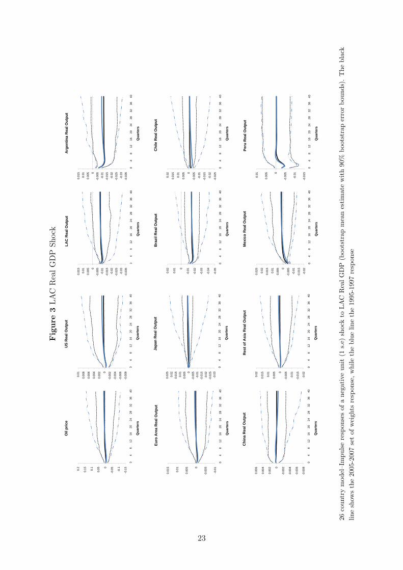
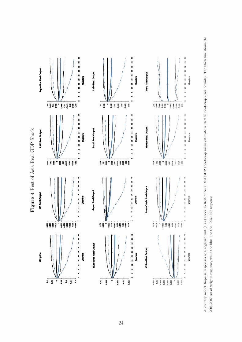
4.1 A Regional GDP Shock in LAC and the Rest of Emerging Asia
Consider first a one standard deviation negative shock to LAC GDP. This shock is con-
structed as the PPP-GDP average of output shocks originated in Latin American country-
specific models and it is equivalent to a decline of LAC GDP of 0.8 percent per quarter under
both set of trade weights.
As presented in Figure 3, the output response in all other countries and regions is not
statistically different from zero, which is not surprising given the region’s relatively small share
in global trade and output. More importantly, though, the effects on LAC itself are virtually
unchanged with 2005-07 trade weights, compared to the 1995-97 weights.
By looking at individual country responses, the short-run reaction of output in Chile is
slightly smaller with more recent trade weights, while the response of Argentina appears to
be slightly stronger. But these differences are very small and are dwarfed by the responses of
Brazil and Mexico, given their relative importance in LAC’s total output (45 and 32 percent,
respectively) and the small number of LAC countries considered. It is interesting to contrast
these responses with those originated by a shock to emerging Asia, which is a traditional
comparator for the five LAC countries we consider. Like a LAC regional shock, a regional GDP
shock in the rest of emerging Asia (excluding China and India) has a similar zero impact on
the rest of the world with 2005-07 trade weights. Unlike a LAC regional shock, however, with
1995-97 trade weights, a regional shocks to the rest of emerging Asia does have a much larger
impact on the rest of the world, albeit estimated very imprecisely, and hence a larger effect on
the region itself.
The two set of results speak to an extent to the much-debated ”decoupling” hypothesis.
According to this hypothesis, emerging markets have decoupled from more advanced economies
in recent years in the sense that their growth performance is less affected by growth at the center
of the world economy and more affected by its own internal dynamics, in part also due to the
process of globalization. In terms of the response of LAC and the rest of emerging Asia to
a regional shock, this should translate into a larger sensitivity of regional output to shocks
emanating in the region itself and smaller responses to shocks emanating outside the region.
The results reported, however, suggest the that the significant changes in the geographical
distribution of international trade that we documented in the paper are not associated with a
major increase in the importance of regional shocks for these two regions themselves. While
this evidence is not necessarily inconsistent with the decoupling hypothesis, it does suggest
that, if decoupling is taking place, it is not going through a key component of the globalization
process: the changed geographical patterns of international trade. In this sense, these results
lend no support to the decoupling hypothesis.
14
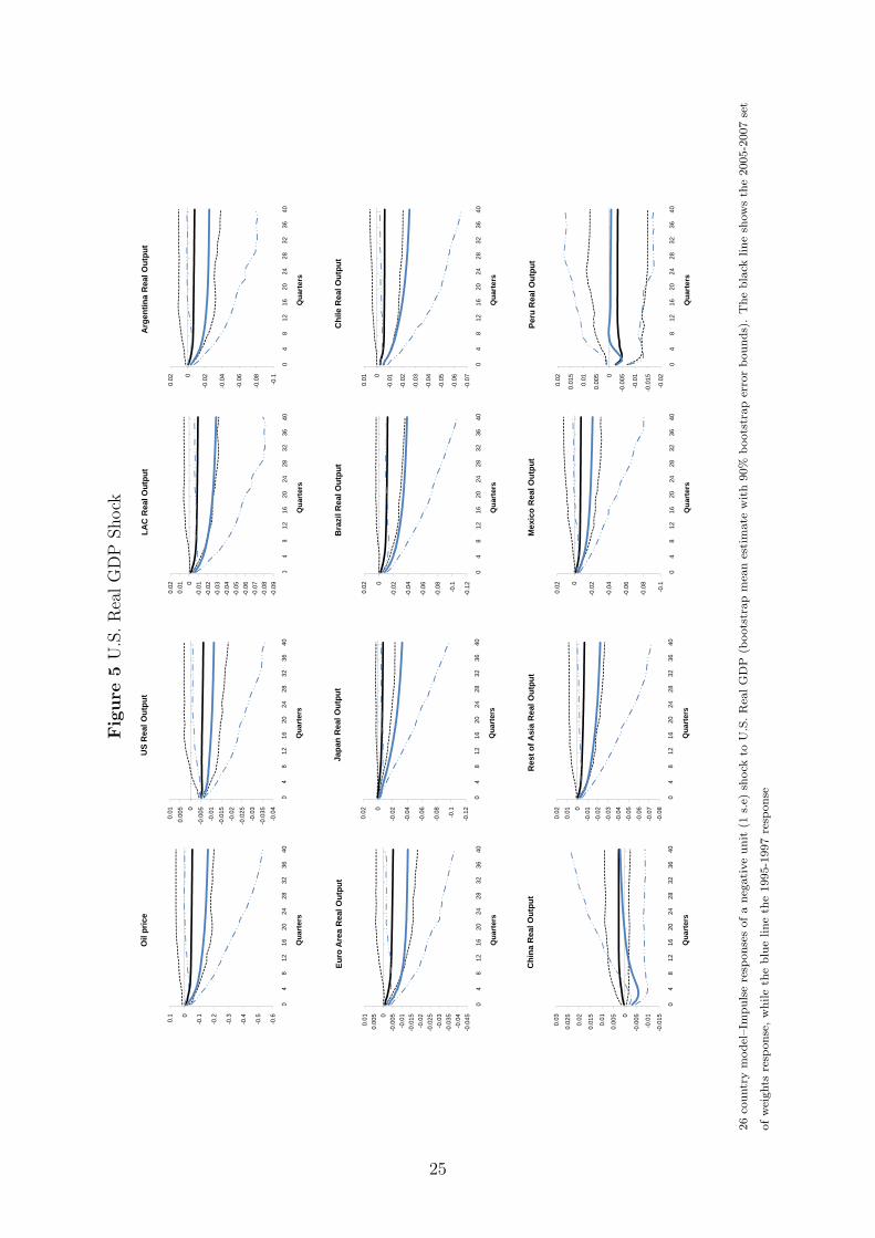
4.2 A U.S. GDP Shock
Figure 5 presents the GIRF to a negative one standard error shock to U.S. output, which is
equivalent to a GDP fall of about 0.5% on impact. Nonetheless, with the 2005-07 weights, the
medium term effect of the shock on U.S. GDP is about half the size of the impact with 1995-97
weights at about -0,5% in the first two years. Thereafter it ceases to be statistically significant.
This evidence is consistent with the so-called ”great moderation” hypothesis according to which
the U.S. economy has become less volatile and more resilient to shocks because of its flexibility
and its full integration in the globalization process. In terms of the U.S. response to domestic
shocks this may translate in smaller impacts as we find.
Looking at the impact of the U.S. shocks on other countries and regions, it is notable that the
effects with 2005-07 trade weights are smaller in all cases reported. Particularly interesting are
the cases of China and the LAC. In the case of China, the response with 2005-07 trade weights
is not statistically significant, while it is much more pronounced and statistically significant
with 1995-97 trade weights.
LAC’s response is smaller with more recent trade weights, right after the first quarter, and
the difference gets larger in the long run, although it ceases to be statistically significant after
eight quarters. At the 2-year horizon output in the region falls by 0.7% (so the multiplier is
still larger than one), which is less than half of what it is with 1995-97 trade shares.
Notable is also the effect of a U.S. output shock on oil prices, which is an endogenous
variable in the U.S. model. As we can see, the oil price response is also smaller with 2005-07
trade weights, which helps to explain why the decrease of the impact of the shock on other
countries is even larger than in the case of the U.S..
These results have an important implications for the puzzles raised by the recent global
financial and economic crisis. In fact they suggest that one reason why economies not located
at the epicenter of the crisis recovered so quickly, is that they are now less affected by U.S. GDP
shocks, which in turn seems largely due to the fact that the U.S. itself is now significantly more
stable than in the past. This in turn suggests that while the great moderation may ultimately
prove to have been temporary, its presence and working up to the onset of the crisis may help
understanding why the global recovery was almost as precipitous as the global slump in the
2008Q4 and 2009Q1.
4.3 A Euro Area GDP Shock
Figure 6 displays a negative one-standard deviation shock to output in the euro area, corre-
sponding to a decline of euro area real GDP of 0.3% on impact and of about 0.5% per quarter
in the first two years, both for the recent and the past set of trade weights. Output response
in most other countries and regions is statistically insignificant, except for the euro area itself.
Note however that, although insignificant, the responses in LAC and ”rest of Asia” are smaller
with 2005-07 than with 1995-97 trade weights under the recent trade shares. In LAC, in partic-
15
ular, the long run (at 2-3-year horizon) is about 30% smaller than with 1995-97 trade weights,
and it is rather homogeneous across LAC countries.
4.4 A China GDP Shock
Figure 7 reports a negative one-standard deviation shock to China’s output. The shock
amounts to a 0,6% fall in China’s real GDP on impact and peaks at -1% after a year, with both
the 1995-97 and the 2005-07 set of weights. With 2005-07 trade weights, however, the shock is
more persistent and its long run impact is larger.
The impact of the shocks on all other countries and regions is larger except in the case
of Japan. In the United States, in particular, the response is remarkably larger and more
persistent: at its peak, output contracts by 0.6%, compared to about 0.3% with 1995-97 trade
weights. Via its effects on the U.S. economy, the shock to China GDP has larger effects also
on the oil price with more recent trade weights.
LAC output, and especially Argentina and Brazil, responds in a similar fashion reflecting
the importance of the indirect effects via the impact on the United States. Interestingly, even
in the case of a shock to China, Chile becomes virtually isolated with 2005-07 trade weights,
while Mexico is surprisingly immune to the shocks despite its strong ties with the U.S. economy
and the importance of oil for the economy.
The response to a GDP shock in China also helps to understand why economies not located
at the epicenter of the crisis recovered so quickly: with more recent trade weights, the world
economy is more responsive to China GDP and relatively less responsive to U.S. GDP compared
to the 1995-97 period. As China GDP has recovered much faster than U.S. GDP one would
expect those economies not at the epicenter of the global crisis to recover faster than in the
past.
4.5 A Global GDP Shock
Consider finally a one-standard deviation negative shock to global output reported in Figure
8. Such a shock can be interpreted as an autonomous change in global GDP triggered by either
a demand or a supply disturbance. The shock amounts to a fall on impact of about 0.4% per
quarter in global output and about -1.55% and -0.89% with 1995-97 and 2005-07 trade weights,
respectively in the long run.14
In the case of China, the response to the global shock is larger with 2005-07 than with
1995-97 trade shares, at 0.7% and about zero, respectively. Possibly, this is due to the larger
effect of domestic shocks consistent with a decoupling hypothesis. In the case of the United
States, instead, a larger impact of shocks from China is offset by a smaller impact of domestic
shocks. As a result, the impact on the United States is essentially unchanged.
14To evaluate the fall in global output, we aggregate all the country-specific GDP impulse responses using asweights the GDP-PPP shares in global output.
16
In the case of LAC the impact of the shock more than halves in the long run, from about
0.3% with 1995-97 trade weights to about 0.15% with 2005-07 trade weights. This pattern is
common across three of the five countries in the region, with Peru and Chile exhibiting the
highest and the lowest exposure, respectively.
For all countries and regions except the US and China, the impact of the shock is signifi-
cantly smaller with 2005-07 than with 1995-97 trade weights. Based on the discussion of the
transmission of regional and country-specific shocks, the results likely reflect the offsetting in-
fluences of the larger impact of GDP shocks from China and smaller impact of GDP shocks
from the United States, with the latter dominating the transmission of the global shock. In
fact, while trade shares of most countries with China have increased very sharply from mid-
1990s to mid-2000s (alongside with the spectacular increase in the degree of openness of the
Chinese economy), the United States remains a very large trade partner for most economies of
the world.
Nonetheless, looking forward, it is likely that the trade share of China will continue to grow
over time. The analysis of the transmission of a global GDP shock therefore suggests that, if
the globalization process were to continue with the same international trade patterns realized
in recent years, it is possible that the world economy will become more volatile possibly because
more affected by China’s own GDP dynamics.
5 Conclusions
In this paper we investigate how China’s emergence in the world economy may have changed
the transmission of global output shocks to the Latin America region and the rest of the world
economy. Based on a GVAR model for the 26 largest emerging and advanced economies of
the world, estimated with an updated dataset up to 2008Q2, we conducted a counterfactual
exercise in which the same shocks were simulated with the same model specification but under
two different sets of trade weights, based on 1995-97 and 2005-07 average trade data.
We found that the impact of a global GDP shock has almost halved in the case of LAC,
and has fallen significantly in all other major countries and region of the world, except China
and the United States. We interpreted this finding as reflecting the fact that China and the US
have become, respectively, more and less responsive to their own output shock. This evidence
is consistent with the decoupling hypothesis for the case of China and the great moderation
hypothesis for the case of the United States.
The evidence reported in the paper helps to understand the pattern of global recovery ob-
served in the aftermath of the global crisis, and in particular why emerging markets such as
the Latin American economies we considered have recovered much faster than initially antic-
ipated. The empirical analysis in the paper also has implications for the future evolution of
world economy. To the extent to which, going forward, the world economy will load more on
China and less on the US, it is likely to become more volatile, at least in the medium term.
17
The analysis of the same counterfactual exercise changing both the model specification and
the trade weights is an important area of further work.
18
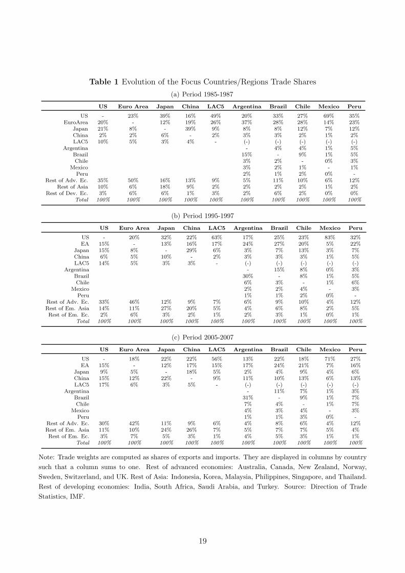
Table 1 Evolution of the Focus Countries/Regions Trade Shares
(a) Period 1985-1987
US Euro Area Japan China LAC5 Argentina Brazil Chile Mexico Peru
US - 23% 39% 16% 49% 20% 33% 27% 69% 35%EuroArea 20% - 12% 19% 26% 37% 28% 28% 14% 23%
Japan 21% 8% - 39% 9% 8% 8% 12% 7% 12%China 2% 2% 6% - 2% 3% 3% 2% 1% 2%LAC5 10% 5% 3% 4% - (-) (-) (-) (-) (-)
Argentina - 4% 4% 1% 5%Brazil 15% - 9% 1% 5%Chile 3% 2% - 0% 3%
Mexico 3% 2% 1% - 1%Peru 2% 1% 2% 0% -
Rest of Adv. Ec. 35% 50% 16% 13% 9% 5% 11% 10% 6% 12%Rest of Asia 10% 6% 18% 9% 2% 2% 2% 2% 1% 2%
Rest of Dev. Ec. 3% 6% 6% 1% 3% 2% 6% 2% 0% 0%Total 100% 100% 100% 100% 100% 100% 100% 100% 100% 100%
(b) Period 1995-1997
US Euro Area Japan China LAC5 Argentina Brazil Chile Mexico Peru
US - 20% 32% 22% 63% 17% 25% 23% 83% 32%EA 15% - 13% 16% 17% 24% 27% 20% 5% 22%
Japan 15% 8% - 29% 6% 3% 7% 13% 3% 7%China 6% 5% 10% - 2% 3% 3% 3% 1% 5%LAC5 14% 5% 3% 3% - (-) (-) (-) (-) (-)
Argentina - 15% 8% 0% 3%Brazil 30% - 8% 1% 5%Chile 6% 3% - 1% 6%
Mexico 2% 2% 4% - 3%Peru 1% 1% 2% 0% -
Rest of Adv. Ec. 33% 46% 12% 9% 7% 6% 9% 10% 4% 12%Rest of Em. Asia 14% 11% 27% 20% 5% 4% 6% 8% 2% 5%Rest of Em. Ec. 2% 6% 3% 2% 1% 2% 3% 1% 0% 1%
Total 100% 100% 100% 100% 100% 100% 100% 100% 100% 100%
(c) Period 2005-2007
US Euro Area Japan China LAC5 Argentina Brazil Chile Mexico Peru
US - 18% 22% 22% 56% 13% 22% 18% 71% 27%EA 15% - 12% 17% 15% 17% 24% 21% 7% 16%
Japan 9% 5% - 18% 5% 2% 4% 9% 4% 6%China 15% 12% 22% - 9% 11% 10% 13% 6% 13%LAC5 17% 6% 3% 5% - (-) (-) (-) (-) (-)
Argentina - 11% 7% 1% 3%Brazil 31% - 9% 1% 7%Chile 7% 4% - 1% 7%
Mexico 4% 3% 4% - 3%Peru 1% 1% 3% 0% -
Rest of Adv. Ec. 30% 42% 11% 9% 6% 4% 8% 6% 4% 12%Rest of Em. Asia 11% 10% 24% 26% 7% 5% 7% 7% 5% 4%Rest of Em. Ec. 3% 7% 5% 3% 1% 4% 5% 3% 1% 1%
Total 100% 100% 100% 100% 100% 100% 100% 100% 100% 100%
Note: Trade weights are computed as shares of exports and imports. They are displayed in columns by countrysuch that a column sums to one. Rest of advanced economies: Australia, Canada, New Zealand, Norway,Sweden, Switzerland, and UK. Rest of Asia: Indonesia, Korea, Malaysia, Philippines, Singapore, and Thailand.Rest of developing economies: India, South Africa, Saudi Arabia, and Turkey. Source: Direction of TradeStatistics, IMF.
19
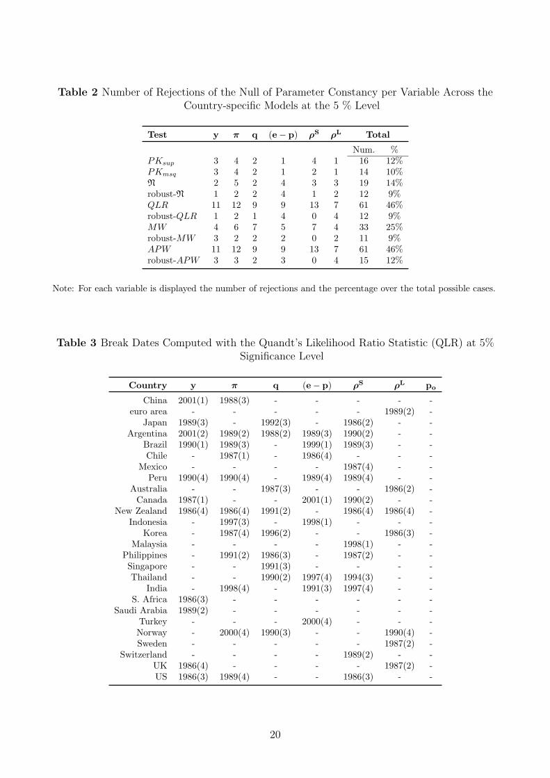
Table 2 Number of Rejections of the Null of Parameter Constancy per Variable Across theCountry-specific Models at the 5 % Level
Test y π q (e− p) ρS ρL Total
Num. %PKsup 3 4 2 1 4 1 16 12%PKmsq 3 4 2 1 2 1 14 10%N 2 5 2 4 3 3 19 14%robust-N 1 2 2 4 1 2 12 9%QLR 11 12 9 9 13 7 61 46%robust-QLR 1 2 1 4 0 4 12 9%MW 4 6 7 5 7 4 33 25%robust-MW 3 2 2 2 0 2 11 9%APW 11 12 9 9 13 7 61 46%robust-APW 3 3 2 3 0 4 15 12%
Note: For each variable is displayed the number of rejections and the percentage over the total possible cases.
Table 3 Break Dates Computed with the Quandt’s Likelihood Ratio Statistic (QLR) at 5%Significance Level
Country y π q (e− p) ρS ρL po
China 2001(1) 1988(3) - - - - -euro area - - - - - 1989(2) -
Japan 1989(3) - 1992(3) - 1986(2) - -Argentina 2001(2) 1989(2) 1988(2) 1989(3) 1990(2) - -
Brazil 1990(1) 1989(3) - 1999(1) 1989(3) - -Chile - 1987(1) - 1986(4) - - -
Mexico - - - - 1987(4) - -Peru 1990(4) 1990(4) - 1989(4) 1989(4) - -
Australia - - 1987(3) - - 1986(2) -Canada 1987(1) - - 2001(1) 1990(2) - -
New Zealand 1986(4) 1986(4) 1991(2) - 1986(4) 1986(4) -Indonesia - 1997(3) - 1998(1) - - -
Korea - 1987(4) 1996(2) - - 1986(3) -Malaysia - - - - 1998(1) - -
Philippines - 1991(2) 1986(3) - 1987(2) - -Singapore - - 1991(3) - - - -Thailand - - 1990(2) 1997(4) 1994(3) - -
India - 1998(4) - 1991(3) 1997(4) - -S. Africa 1986(3) - - - - - -
Saudi Arabia 1989(2) - - - - - -Turkey - - - 2000(4) - - -Norway - 2000(4) 1990(3) - - 1990(4) -Sweden - - - - - 1987(2) -
Switzerland - - - - 1989(2) - -UK 1986(4) - - - - 1987(2) -US 1986(3) 1989(4) - - 1986(3) - -
20
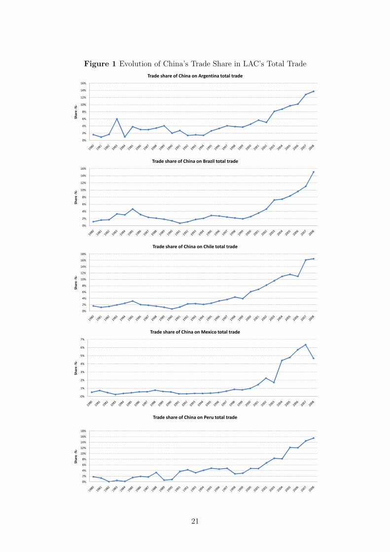
Figure 1 Evolution of China’s Trade Share in LAC’s Total Trade
0%
2%
4%
6%
8%
10%
12%
14%
16%
Sh
are
-%
-Trade share of China on Argentina total trade
0%
2%
4%
6%
8%
10%
12%
14%
16%
Sh
are
-%
-
Trade share of China on Brazil total trade
12%
14%
16%
18%
Trade share of China on Chile total trade
0%
2%
4%
6%
8%
10%
12%
Sh
are
-%
-
0%
1%
2%
3%
4%
5%
6%
7%
Sh
are
-%
-
Trade share of China on Mexico total trade
0%
2%
4%
6%
8%
10%
12%
14%
16%
18%
Sh
are
-%
-
Trade share of China on Peru total trade
21
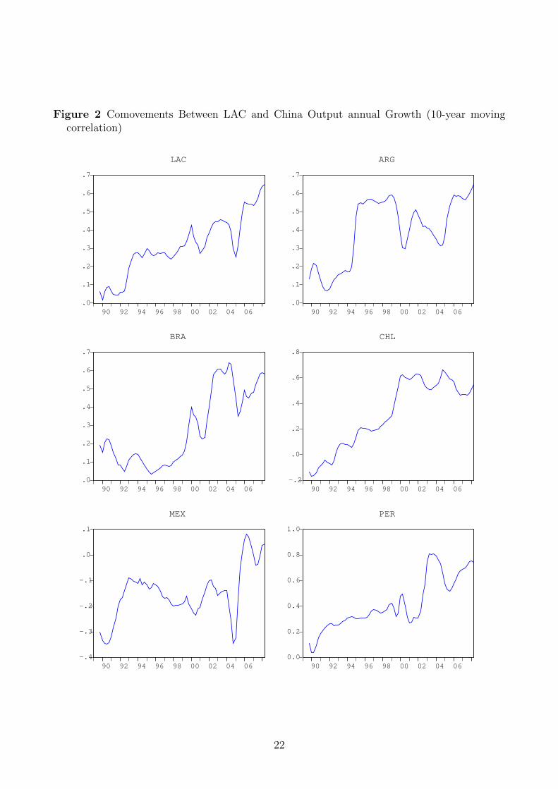
Figure 2 Comovements Between LAC and China Output annual Growth (10-year movingcorrelation)
.0
.1
.2
.3
.4
.5
.6
.7
90 92 94 96 98 00 02 04 06
LAC
.0
.1
.2
.3
.4
.5
.6
.7
90 92 94 96 98 00 02 04 06
ARG
.0
.1
.2
.3
.4
.5
.6
.7
90 92 94 96 98 00 02 04 06
BRA
-.2
.0
.2
.4
.6
.8
90 92 94 96 98 00 02 04 06
CHL
-.4
-.3
-.2
-.1
.0
.1
90 92 94 96 98 00 02 04 06
MEX
0.0
0.2
0.4
0.6
0.8
1.0
90 92 94 96 98 00 02 04 06
PER
22
Fig
ure
3LA
CR
ealG
DP
Shock
-0.0
35
-0.0
3
-0.0
25
-0.0
2
-0.0
15
-0.0
1
-0.0
050
0.00
5
0.01
0.01
5
04
812
1620
2428
3236
40
LA
C R
eal O
utp
ut
-0.0
35
-0.0
3
-0.0
25
-0.0
2
-0.0
15
-0.0
1
-0.0
050
0.00
5
0.01
0.01
5
04
812
1620
2428
3236
40
Arg
enti
na
Rea
l Ou
tpu
t
-0.1
5
-0.1
-0.0
50
0.050.1
0.150.2
04
812
1620
2428
3236
40
Oil
pri
ce
-0.0
08
-0.0
06
-0.0
04
-0.0
020
0.00
2
0.00
4
0.00
6
0.00
8
0.01
04
812
1620
2428
3236
40
US
Rea
l Ou
tpu
t
-0.0
5
-0.0
4
-0.0
3
-0.0
2
-0.0
10
0.01
0.02
04
812
1620
2428
3236
40
Qu
arte
rs
Bra
zil R
eal O
utp
ut
-0.0
25
-0.0
2
-0.0
15
-0.0
1
-0.0
050
0.00
5
0.01
0.01
5
0.02
04
812
1620
2428
3236
40
Qu
arte
rs
Ch
ile R
eal O
utp
ut
04
812
1620
2428
3236
40
Qu
arte
rs
04
812
1620
2428
3236
40
Qu
arte
rs
04
812
1620
2428
3236
40
Qu
arte
rs
-0.0
3
-0.0
25
-0.0
2
-0.0
15
-0.0
1
-0.0
050
0.00
5
0.01
0.01
5
0.02
0.02
5
04
812
1620
2428
3236
40
Qu
arte
rs
Jap
an R
eal O
utp
ut
04
812
1620
2428
3236
40
Qu
arte
rs
-0.0
1
-0.0
050
0.00
5
0.01
0.01
5
04
812
1620
2428
3236
40
Qu
arte
rs
Eu
ro A
rea
Rea
l Ou
tpu
t
-0.0
2
-0.0
15
-0.0
1
-0.0
050
0.00
5
0.01
0.01
5
0.02
0.02
5
04
812
1620
2428
3236
40
Qu
arte
rs
Mex
ico
Rea
l Ou
tpu
t
-0.0
15
-0.0
1
-0.0
050
0.00
5
0.01
04
812
1620
2428
3236
40
Qu
arte
rs
Per
u R
eal O
utp
ut
-0.0
08
-0.0
06
-0.0
04
-0.0
020
0.00
2
0.00
4
0.00
6
04
812
1620
2428
3236
40
Qu
arte
rs
Ch
ina
Rea
l Ou
tpu
t
-0.0
2
-0.0
15
-0.0
1
-0.0
050
0.00
5
0.01
0.01
5
0.02
04
812
1620
2428
3236
40
Qu
arte
rs
Res
t o
f A
sia
Rea
l Ou
tpu
t
26co
untr
ym
odel
–Im
puls
ere
spon
ses
ofa
nega
tive
unit
(1s.
e)sh
ock
toLA
CR
ealG
DP
(boo
tstr
apm
ean
esti
mat
ew
ith
90%
boot
stra
per
ror
boun
ds).
The
blac
klin
esh
ows
the
2005
-200
7se
tof
wei
ghts
resp
onse
,w
hile
the
blue
line
the
1995
-199
7re
spon
se
23
Fig
ure
4R
est
ofA
sia
Rea
lG
DP
Shock
LAC
Rea
l Out
put
Arg
entin
a R
eal O
utpu
tO
il pr
ice
US
Rea
l Out
put
-0.0
1
-0.0
050
0.00
5
0.01
0.01
5
LAC
Rea
l Out
put
-001
-0.0
0500.
005
0.01
0.01
50.
02
Arg
entin
a R
eal O
utpu
t
-0.0
50
0.050.1
Oil
pric
e
-000
4-0
.0020
0.00
20.
004
0.00
60.
008
US
Rea
l Out
put
-0.0
3
-0.0
25
-0.0
2
-0.0
15
-0.0
1
-0.0
050
0.00
5
0.01
0.01
5
04
812
1620
2428
3236
40
Qua
rter
s
LAC
Rea
l Out
put
-0.0
3-0
.025
-0.0
2-0
.015
-0.0
1-0
.0050
0.00
50.
010.
015
0.02
04
812
1620
2428
3236
40
Qua
rter
s
Arg
entin
a R
eal O
utpu
t
-0.2
-0.1
5
-0.1
-0.0
50
0.050.1
04
812
1620
2428
3236
40
Qua
rter
s
Oil
pric
e
-0.0
12-0
.01
-0.0
08-0
.006
-0.0
04-0
.0020
0.00
20.
004
0.00
60.
008
04
812
1620
2428
3236
40
Qua
rter
s
US
Rea
l Out
put
00.
005
0.01
0.01
5
Bra
zil R
eal O
utpu
t
0
0.00
5
0.01
Chi
le R
eal O
utpu
t
-0.0
3
-0.0
25
-0.0
2
-0.0
15
-0.0
1
-0.0
050
0.00
5
0.01
0.01
5
04
812
1620
2428
3236
40
Qua
rter
s
LAC
Rea
l Out
put
-0.0
3-0
.025
-0.0
2-0
.015
-0.0
1-0
.0050
0.00
50.
010.
015
0.02
04
812
1620
2428
3236
40
Qua
rter
s
Arg
entin
a R
eal O
utpu
t
-0.2
-0.1
5
-0.1
-0.0
50
0.050.1
04
812
1620
2428
3236
40
Qua
rter
s
Oil
pric
e
-0.0
0500.
005
0.01
Japa
n R
eal O
utpu
t
-0.0
12-0
.01
-0.0
08-0
.006
-0.0
04-0
.0020
0.00
20.
004
0.00
60.
008
04
812
1620
2428
3236
40
Qua
rter
s
US
Rea
l Out
put
0.00
5
0.01
Euro
Are
a R
eal O
utpu
t
-0.0
35-0
.03
-0.0
25-0
.02
-0.0
15-0
.01
-0.0
0500.
005
0.01
0.01
5
04
812
1620
2428
3236
40
Bra
zil R
eal O
utpu
t
-0.0
3
-0.0
25
-0.0
2
-0.0
15
-0.0
1
-0.0
050
0.00
5
0.01
04
812
1620
2428
3236
40
Chi
le R
eal O
utpu
t
-0.0
3
-0.0
25
-0.0
2
-0.0
15
-0.0
1
-0.0
050
0.00
5
0.01
0.01
5
04
812
1620
2428
3236
40
Qua
rter
s
LAC
Rea
l Out
put
-0.0
3-0
.025
-0.0
2-0
.015
-0.0
1-0
.0050
0.00
50.
010.
015
0.02
04
812
1620
2428
3236
40
Qua
rter
s
Arg
entin
a R
eal O
utpu
t
-0.2
-0.1
5
-0.1
-0.0
50
0.050.1
04
812
1620
2428
3236
40
Qua
rter
s
Oil
pric
e
-0.0
4-0
.035
-0.0
3-0
.025
-0.0
2-0
.015
-0.0
1-0
.0050
0.00
50.
01
04
812
1620
2428
3236
40
Japa
n R
eal O
utpu
t
-0.0
12-0
.01
-0.0
08-0
.006
-0.0
04-0
.0020
0.00
20.
004
0.00
60.
008
04
812
1620
2428
3236
40
Qua
rter
s
US
Rea
l Out
put
-0.0
15
-0.0
1
-0.0
050
0.00
5
0.01
04
812
1620
2428
3236
40
Euro
Are
a R
eal O
utpu
t
-0.0
35-0
.03
-0.0
25-0
.02
-0.0
15-0
.01
-0.0
0500.
005
0.01
0.01
5
04
812
1620
2428
3236
40
Qua
rter
s
Bra
zil R
eal O
utpu
t
-0.0
3
-0.0
25
-0.0
2
-0.0
15
-0.0
1
-0.0
050
0.00
5
0.01
04
812
1620
2428
3236
40
Qua
rter
s
Chi
le R
eal O
utpu
t
-0.0
3
-0.0
25
-0.0
2
-0.0
15
-0.0
1
-0.0
050
0.00
5
0.01
0.01
5
04
812
1620
2428
3236
40
Qua
rter
s
LAC
Rea
l Out
put
-0.0
3-0
.025
-0.0
2-0
.015
-0.0
1-0
.0050
0.00
50.
010.
015
0.02
04
812
1620
2428
3236
40
Qua
rter
s
Arg
entin
a R
eal O
utpu
t
0.01
5
Mex
ico
Rea
l Out
put
0.01
Peru
Rea
l Out
put
-0.2
-0.1
5
-0.1
-0.0
50
0.050.1
04
812
1620
2428
3236
40
Qua
rter
s
Oil
pric
e
-0.0
4-0
.035
-0.0
3-0
.025
-0.0
2-0
.015
-0.0
1-0
.0050
0.00
50.
01
04
812
1620
2428
3236
40
Qua
rter
s
Japa
n R
eal O
utpu
t
-0.0
12-0
.01
-0.0
08-0
.006
-0.0
04-0
.0020
0.00
20.
004
0.00
60.
008
04
812
1620
2428
3236
40
Qua
rter
s
US
Rea
l Out
put
0.01
2
Chi
na R
eal O
utpu
t
0.01
Res
t of A
sia
Rea
l Out
put
-0.0
15
-0.0
1
-0.0
050
0.00
5
0.01
04
812
1620
2428
3236
40
Qua
rter
s
Euro
Are
a R
eal O
utpu
t
-0.0
35-0
.03
-0.0
25-0
.02
-0.0
15-0
.01
-0.0
0500.
005
0.01
0.01
5
04
812
1620
2428
3236
40
Qua
rter
s
Bra
zil R
eal O
utpu
t
-0.0
3
-0.0
25
-0.0
2
-0.0
15
-0.0
1
-0.0
050
0.00
5
0.01
04
812
1620
2428
3236
40
Qua
rter
s
Chi
le R
eal O
utpu
t
-0.0
3
-0.0
25
-0.0
2
-0.0
15
-0.0
1
-0.0
050
0.00
5
0.01
0.01
5
04
812
1620
2428
3236
40
Qua
rter
s
LAC
Rea
l Out
put
-0.0
3-0
.025
-0.0
2-0
.015
-0.0
1-0
.0050
0.00
50.
010.
015
0.02
04
812
1620
2428
3236
40
Qua
rter
s
Arg
entin
a R
eal O
utpu
t
-0.0
2
-0.0
15
-0.0
1
-0.0
050
0.00
5
0.01
0.01
5
Mex
ico
Rea
l Out
put
-000
6-0
.004
-0.0
0200.
002
0.00
40.
006
0.00
80.
01
Peru
Rea
l Out
put
-0.2
-0.1
5
-0.1
-0.0
50
0.050.1
04
812
1620
2428
3236
40
Qua
rter
s
Oil
pric
e
-0.0
4-0
.035
-0.0
3-0
.025
-0.0
2-0
.015
-0.0
1-0
.0050
0.00
50.
01
04
812
1620
2428
3236
40
Qua
rter
s
Japa
n R
eal O
utpu
t
-0.0
12-0
.01
-0.0
08-0
.006
-0.0
04-0
.0020
0.00
20.
004
0.00
60.
008
04
812
1620
2428
3236
40
Qua
rter
s
US
Rea
l Out
put
0
0.00
2
0.00
4
0.00
6
0.00
8
0.01
0.01
2
Chi
na R
eal O
utpu
t
-0.0
25
-0.0
2
-0.0
15
-0.0
1
-0.0
050
0.00
5
0.01
Res
t of A
sia
Rea
l Out
put
-0.0
15
-0.0
1
-0.0
050
0.00
5
0.01
04
812
1620
2428
3236
40
Qua
rter
s
Euro
Are
a R
eal O
utpu
t
-0.0
35-0
.03
-0.0
25-0
.02
-0.0
15-0
.01
-0.0
0500.
005
0.01
0.01
5
04
812
1620
2428
3236
40
Qua
rter
s
Bra
zil R
eal O
utpu
t
-0.0
3
-0.0
25
-0.0
2
-0.0
15
-0.0
1
-0.0
050
0.00
5
0.01
04
812
1620
2428
3236
40
Qua
rter
s
Chi
le R
eal O
utpu
t
-0.0
3
-0.0
25
-0.0
2
-0.0
15
-0.0
1
-0.0
050
0.00
5
0.01
0.01
5
04
812
1620
2428
3236
40
Qua
rter
s
LAC
Rea
l Out
put
-0.0
3-0
.025
-0.0
2-0
.015
-0.0
1-0
.0050
0.00
50.
010.
015
0.02
04
812
1620
2428
3236
40
Qua
rter
s
Arg
entin
a R
eal O
utpu
t
-0.0
3
-0.0
25
-0.0
2
-0.0
15
-0.0
1
-0.0
050
0.00
5
0.01
0.01
5
04
812
1620
2428
3236
40
Qua
rter
s
Mex
ico
Rea
l Out
put
-0.0
1-0
.008
-0.0
06-0
.004
-0.0
0200.
002
0.00
40.
006
0.00
80.
01
04
812
1620
2428
3236
40
Qua
rter
s
Peru
Rea
l Out
put
-0.2
-0.1
5
-0.1
-0.0
50
0.050.1
04
812
1620
2428
3236
40
Qua
rter
s
Oil
pric
e
-0.0
4-0
.035
-0.0
3-0
.025
-0.0
2-0
.015
-0.0
1-0
.0050
0.00
50.
01
04
812
1620
2428
3236
40
Qua
rter
s
Japa
n R
eal O
utpu
t
-0.0
12-0
.01
-0.0
08-0
.006
-0.0
04-0
.0020
0.00
20.
004
0.00
60.
008
04
812
1620
2428
3236
40
Qua
rter
s
US
Rea
l Out
put
-0.0
04
-0.0
020
0.00
2
0.00
4
0.00
6
0.00
8
0.01
0.01
2
04
812
1620
2428
3236
40
Qua
rter
s
Chi
na R
eal O
utpu
t
-0.0
35
-0.0
3
-0.0
25
-0.0
2
-0.0
15
-0.0
1
-0.0
050
0.00
5
0.01
04
812
1620
2428
3236
40
Qua
rter
s
Res
t of A
sia
Rea
l Out
put
-0.0
15
-0.0
1
-0.0
050
0.00
5
0.01
04
812
1620
2428
3236
40
Qua
rter
s
Euro
Are
a R
eal O
utpu
t
26
countr
ym
odel
–Im
puls
ere
sponse
sofa
neg
ative
unit
(1s.
e)sh
ock
toR
est
ofA
sia
Rea
lG
DP
(boots
trap
mea
nes
tim
ate
wit
h90%
boots
trap
erro
rbounds)
.T
he
bla
ckline
show
sth
e
2005-2
007
set
ofw
eights
resp
onse
,w
hile
the
blu
eline
the
1995-1
997
resp
onse
24
Fig
ure
5U
.S.R
ealG
DP
Shock
-0.0
9
-0.0
8
-0.0
7
-0.0
6
-0.0
5
-0.0
4
-0.0
3
-0.0
2
-0.0
10
0.01
0.02
04
812
1620
2428
3236
40
LA
C R
eal O
utp
ut
-0.1
-0.0
8
-0.0
6
-0.0
4
-0.0
20
0.02
04
812
1620
2428
3236
40
Arg
enti
na
Rea
l Ou
tpu
t
-0.6
-0.5
-0.4
-0.3
-0.2
-0.10
0.1
04
812
1620
2428
3236
40
Oil
pri
ce
-0.0
4
-0.0
35
-0.0
3
-0.0
25
-0.0
2
-0.0
15
-0.0
1
-0.0
050
0.00
5
0.01
04
812
1620
2428
3236
40
US
Rea
l Ou
tpu
t
-0.1
2
-0.1
-0.0
8
-0.0
6
-0.0
4
-0.0
20
0.02
04
812
1620
2428
3236
40
Qu
arte
rs
Bra
zil R
eal O
utp
ut
-0.0
7
-0.0
6
-0.0
5
-0.0
4
-0.0
3
-0.0
2
-0.0
10
0.01
04
812
1620
2428
3236
40
Qu
arte
rs
Ch
ile R
eal O
utp
ut
04
812
1620
2428
3236
40
Qu
arte
rs
04
812
1620
2428
3236
40
Qu
arte
rs
04
812
1620
2428
3236
40
Qu
arte
rs
-0.1
2
-0.1
-0.0
8
-0.0
6
-0.0
4
-0.0
20
0.02
04
812
1620
2428
3236
40
Qu
arte
rs
Jap
an R
eal O
utp
ut
04
812
1620
2428
3236
40
Qu
arte
rs
-0.0
45
-0.0
4
-0.0
35
-0.0
3
-0.0
25
-0.0
2
-0.0
15
-0.0
1
-0.0
050
0.00
5
0.01
04
812
1620
2428
3236
40
Qu
arte
rs
Eu
ro A
rea
Rea
l Ou
tpu
t
-0.1
-0.0
8
-0.0
6
-0.0
4
-0.0
20
0.02
04
812
1620
2428
3236
40
Qu
arte
rs
Mex
ico
Rea
l Ou
tpu
t
-0.0
2
-0.0
15
-0.0
1
-0.0
050
0.00
5
0.01
0.01
5
0.02
04
812
1620
2428
3236
40
Qu
arte
rs
Per
u R
eal O
utp
ut
-0.0
15
-0.0
1
-0.0
050
0.00
5
0.01
0.01
5
0.02
0.02
5
0.03
04
812
1620
2428
3236
40
Qu
arte
rs
Ch
ina
Rea
l Ou
tpu
t
-0.0
8
-0.0
7
-0.0
6
-0.0
5
-0.0
4
-0.0
3
-0.0
2
-0.0
10
0.01
0.02
04
812
1620
2428
3236
40
Qu
arte
rs
Res
t o
f A
sia
Rea
l Ou
tpu
t
26
countr
ym
odel
–Im
puls
ere
sponse
sofa
neg
ative
unit
(1s.
e)sh
ock
toU
.S.R
ealG
DP
(boots
trap
mea
nes
tim
ate
with
90%
boots
trap
erro
rbounds)
.T
he
bla
ckline
show
sth
e2005-2
007
set
ofw
eights
resp
onse
,w
hile
the
blu
eline
the
1995-1
997
resp
onse
25
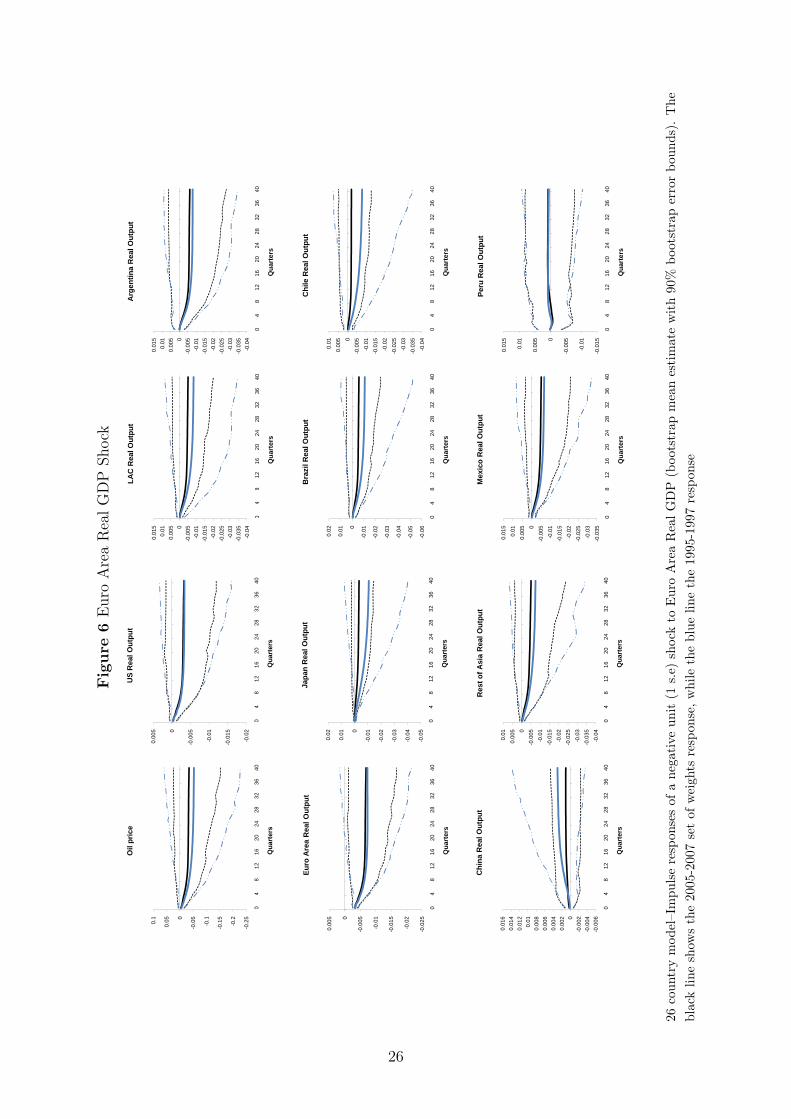
Fig
ure
6E
uro
Are
aR
ealG
DP
Shock
-0.0
4
-0.0
35
-0.0
3
-0.0
25
-0.0
2
-0.0
15
-0.0
1
-0.0
050
0.00
5
0.01
0.01
5
04
812
1620
2428
3236
40
LA
C R
eal O
utp
ut
-0.0
4
-0.0
35
-0.0
3
-0.0
25
-0.0
2
-0.0
15
-0.0
1
-0.0
050
0.00
5
0.01
0.01
5
04
812
1620
2428
3236
40
Arg
enti
na
Rea
l Ou
tpu
t
-0.2
5
-0.2
-0.1
5
-0.1
-0.0
50
0.050.1
04
812
1620
2428
3236
40
Oil
pri
ce
-0.0
2
-0.0
15
-0.0
1
-0.0
050
0.00
5
04
812
1620
2428
3236
40
US
Rea
l Ou
tpu
t
-0.0
6
-0.0
5
-0.0
4
-0.0
3
-0.0
2
-0.0
10
0.01
0.02
04
812
1620
2428
3236
40
Qu
arte
rs
Bra
zil R
eal O
utp
ut
-0.0
4
-0.0
35
-0.0
3
-0.0
25
-0.0
2
-0.0
15
-0.0
1
-0.0
050
0.00
5
0.01
04
812
1620
2428
3236
40
Qu
arte
rs
Ch
ile R
eal O
utp
ut
04
812
1620
2428
3236
40
Qu
arte
rs
04
812
1620
2428
3236
40
Qu
arte
rs
04
812
1620
2428
3236
40
Qu
arte
rs
-0.0
5
-0.0
4
-0.0
3
-0.0
2
-0.0
10
0.01
0.02
04
812
1620
2428
3236
40
Qu
arte
rs
Jap
an R
eal O
utp
ut
04
812
1620
2428
3236
40
Qu
arte
rs
-0.0
25
-0.0
2
-0.0
15
-0.0
1
-0.0
050
0.00
5
04
812
1620
2428
3236
40
Qu
arte
rs
Eu
ro A
rea
Rea
l Ou
tpu
t
-0.0
35
-0.0
3
-0.0
25
-0.0
2
-0.0
15
-0.0
1
-0.0
050
0.00
5
0.01
0.01
5
04
812
1620
2428
3236
40
Qu
arte
rs
Mex
ico
Rea
l Ou
tpu
t
-0.0
15
-0.0
1
-0.0
050
0.00
5
0.01
0.01
5
04
812
1620
2428
3236
40
Qu
arte
rs
Per
u R
eal O
utp
ut
-0.0
06
-0.0
04
-0.0
020
0.00
2
0.00
4
0.00
6
0.00
8
0.01
0.01
2
0.01
4
0.01
6
04
812
1620
2428
3236
40
Qu
arte
rs
Ch
ina
Rea
l Ou
tpu
t
-0.0
4
-0.0
35
-0.0
3
-0.0
25
-0.0
2
-0.0
15
-0.0
1
-0.0
050
0.00
5
0.01
04
812
1620
2428
3236
40
Qu
arte
rs
Res
t o
f A
sia
Rea
l Ou
tpu
t
26co
untr
ym
odel
–Im
puls
ere
spon
ses
ofa
nega
tive
unit
(1s.
e)sh
ock
toE
uro
Are
aR
ealG
DP
(boo
tstr
apm
ean
esti
mat
ew
ith
90%
boot
stra
per
ror
boun
ds).
The
blac
klin
esh
ows
the
2005
-200
7se
tof
wei
ghts
resp
onse
,w
hile
the
blue
line
the
1995
-199
7re
spon
se
26
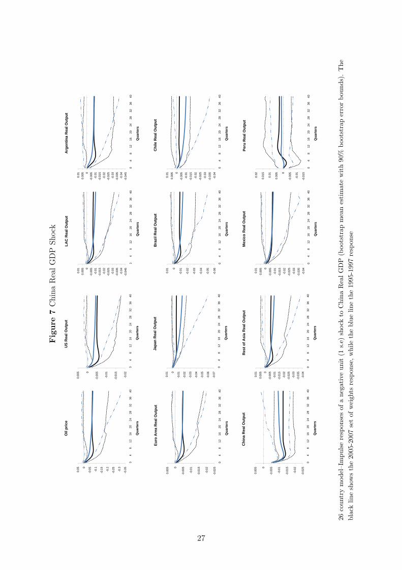
Fig
ure
7C
hin
aR
ealG
DP
Shock
-0.0
45
-0.0
4
-0.0
35
-0.0
3
-0.0
25
-0.0
2
-0.0
15
-0.0
1
-0.0
050
0.00
5
0.01
04
812
1620
2428
3236
40
LA
C R
eal O
utp
ut
-0.0
45
-0.0
4
-0.0
35
-0.0
3
-0.0
25
-0.0
2
-0.0
15
-0.0
1
-0.0
050
0.00
5
0.01
04
812
1620
2428
3236
40
Arg
enti
na
Rea
l Ou
tpu
t
-0.3
5
-0.3
-0.2
5
-0.2
-0.1
5
-0.1
-0.0
50
0.05
04
812
1620
2428
3236
40
Oil
pri
ce
-0.0
2
-0.0
15
-0.0
1
-0.0
050
0.00
5
04
812
1620
2428
3236
40
US
Rea
l Ou
tpu
t
-0.0
6
-0.0
5
-0.0
4
-0.0
3
-0.0
2
-0.0
10
0.01
04
812
1620
2428
3236
40
Qu
arte
rs
Bra
zil R
eal O
utp
ut
-0.0
4
-0.0
35
-0.0
3
-0.0
25
-0.0
2
-0.0
15
-0.0
1
-0.0
050
0.00
5
0.01
04
812
1620
2428
3236
40
Qu
arte
rs
Ch
ile R
eal O
utp
ut
04
812
1620
2428
3236
40
Qu
arte
rs
04
812
1620
2428
3236
40
Qu
arte
rs
04
812
1620
2428
3236
40
Qu
arte
rs
-0.0
7
-0.0
6
-0.0
5
-0.0
4
-0.0
3
-0.0
2
-0.0
10
0.01
04
812
1620
2428
3236
40
Qu
arte
rs
Jap
an R
eal O
utp
ut
04
812
1620
2428
3236
40
Qu
arte
rs
-0.0
25
-0.0
2
-0.0
15
-0.0
1
-0.0
050
0.00
5
04
812
1620
2428
3236
40
Qu
arte
rs
Eu
ro A
rea
Rea
l Ou
tpu
t
-0.0
4
-0.0
35
-0.0
3
-0.0
25
-0.0
2
-0.0
15
-0.0
1
-0.0
050
0.00
5
0.01
04
812
1620
2428
3236
40
Qu
arte
rs
Mex
ico
Rea
l Ou
tpu
t
-0.0
15
-0.0
1
-0.0
050
0.00
5
0.01
0.01
5
0.02
04
812
1620
2428
3236
40
Qu
arte
rs
Per
u R
eal O
utp
ut
-0.0
25
-0.0
2
-0.0
15
-0.0
1
-0.0
050
0.00
5
04
812
1620
2428
3236
40
Qu
arte
rs
Ch
ina
Rea
l Ou
tpu
t
-0.0
4
-0.0
35
-0.0
3
-0.0
25
-0.0
2
-0.0
15
-0.0
1
-0.0
050
0.00
5
0.01
04
812
1620
2428
3236
40
Qu
arte
rs
Res
t o
f A
sia
Rea
l Ou
tpu
t
26co
untr
ym
odel
–Im
puls
ere
spon
ses
ofa
nega
tive
unit
(1s.
e)sh
ock
toC
hina
Rea
lG
DP
(boo
tstr
apm
ean
esti
mat
ew
ith
90%
boot
stra
per
ror
boun
ds).
The
blac
klin
esh
ows
the
2005
-200
7se
tof
wei
ghts
resp
onse
,w
hile
the
blue
line
the
1995
-199
7re
spon
se
27
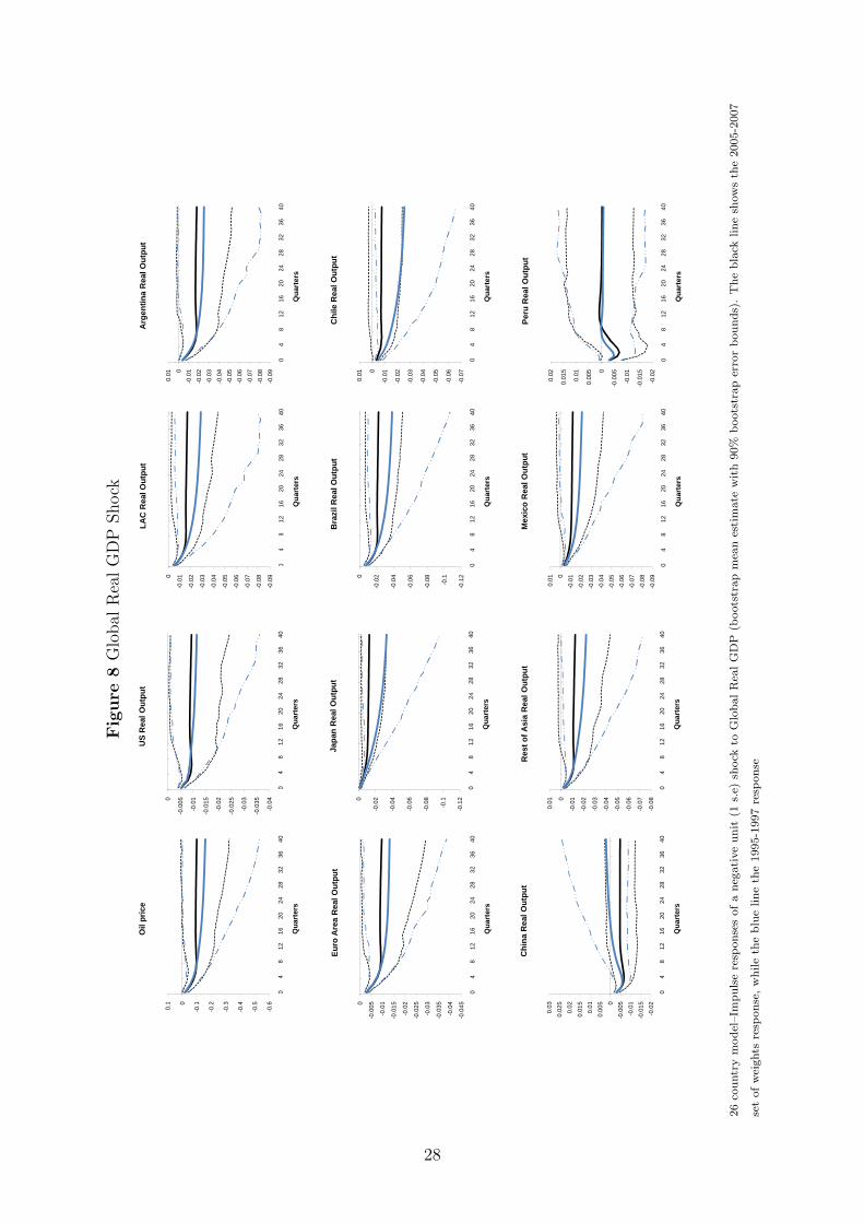
Fig
ure
8G
lobal
Rea
lG
DP
Shock
-0.0
9
-0.0
8
-0.0
7
-0.0
6
-0.0
5
-0.0
4
-0.0
3
-0.0
2
-0.0
10
04
812
1620
2428
3236
40
LA
C R
eal O
utp
ut
-0.0
9
-0.0
8
-0.0
7
-0.0
6
-0.0
5
-0.0
4
-0.0
3
-0.0
2
-0.0
10
0.01
04
812
1620
2428
3236
40
Arg
enti
na
Rea
l Ou
tpu
t
-0.6
-0.5
-0.4
-0.3
-0.2
-0.10
0.1
04
812
1620
2428
3236
40
Oil
pri
ce
-0.0
4
-0.0
35
-0.0
3
-0.0
25
-0.0
2
-0.0
15
-0.0
1
-0.0
050
04
812
1620
2428
3236
40
US
Rea
l Ou
tpu
t
-0.1
2
-0.1
-0.0
8
-0.0
6
-0.0
4
-0.0
20
04
812
1620
2428
3236
40
Qu
arte
rs
Bra
zil R
eal O
utp
ut
-0.0
7
-0.0
6
-0.0
5
-0.0
4
-0.0
3
-0.0
2
-0.0
10
0.01
04
812
1620
2428
3236
40
Qu
arte
rs
Ch
ile R
eal O
utp
ut
04
812
1620
2428
3236
40
Qu
arte
rs
04
812
1620
2428
3236
40
Qu
arte
rs
04
812
1620
2428
3236
40
Qu
arte
rs
-0.1
2
-0.1
-0.0
8
-0.0
6
-0.0
4
-0.0
20
04
812
1620
2428
3236
40
Qu
arte
rs
Jap
an R
eal O
utp
ut
04
812
1620
2428
3236
40
Qu
arte
rs
-0.0
45
-0.0
4
-0.0
35
-0.0
3
-0.0
25
-0.0
2
-0.0
15
-0.0
1
-0.0
050
04
812
1620
2428
3236
40
Qu
arte
rs
Eu
ro A
rea
Rea
l Ou
tpu
t
-0.0
9
-0.0
8
-0.0
7
-0.0
6
-0.0
5
-0.0
4
-0.0
3
-0.0
2
-0.0
10
0.01
04
812
1620
2428
3236
40
Qu
arte
rs
Mex
ico
Rea
l Ou
tpu
t
-0.0
2
-0.0
15
-0.0
1
-0.0
050
0.00
5
0.01
0.01
5
0.02
04
812
1620
2428
3236
40
Qu
arte
rs
Per
u R
eal O
utp
ut
-0.0
2
-0.0
15
-0.0
1
-0.0
050
0.00
5
0.01
0.01
5
0.02
0.02
5
0.03
04
812
1620
2428
3236
40
Qu
arte
rs
Ch
ina
Rea
l Ou
tpu
t
-0.0
8
-0.0
7
-0.0
6
-0.0
5
-0.0
4
-0.0
3
-0.0
2
-0.0
10
0.01
04
812
1620
2428
3236
40
Qu
arte
rs
Res
t o
f A
sia
Rea
l Ou
tpu
t
26
countr
ym
odel
–Im
puls
ere
sponse
sofa
neg
ative
unit
(1s.
e)sh
ock
toG
lobalR
ealG
DP
(boots
trap
mea
nes
tim
ate
with
90%
boots
trap
erro
rbounds)
.T
he
bla
ckline
show
sth
e2005-2
007
set
ofw
eights
resp
onse
,w
hile
the
blu
eline
the
1995-1
997
resp
onse
28

References
Bernanke, B. S. (2009): “Asia and the global financial crisis,” in Federal Reserve Bank of SanFrancisco’s Conference on Asia and the Global Financial Crisis, Santa Barbara, California.FRBSF.
Calderon, C. (2008): “The Growth of China and India Is Not a Zero-Sum Game for LatinAmerica and the Caribbean: Short- and Long-Term Effects,” in China’s and India’s Chal-lenge to Latin America. Opportunity or threat?, ed. by M. Olarreaga, G. Perry, and D. Led-erman, pp. 39–100. The World Bank Press.
Calderon, C., A. Chong, and E. Stein (2007): “Trade intensity and business cycle syn-chronization: Are developing countries any different?,” Journal of International Economics,71(1), 2–21.
Dees, S., F. di Mauro, M. H. Pesaran, and V. Smith (2007): “Exploring the interna-tional linkages of the euro area: a global VAR analysis,” Journal of Applied Econometrics,22(1), 1–38.
Frankel, J. A., and A. K. Rose (1998): “The Endogeneity of the Optimum Currency AreaCriteria,” Economic Journal, 108(449), 1009–25.
Fuller, W., and H. Park (1995): “Alternative Estimators and Unit Root Tests for theAutoregressive Process,” Journal of Time Series Analysis, 16, 415–429.
Galesi, A., and S. Sgherri (2009): “Regional Financial Spillovers Across Europe: A GlobalVAR Analysis,” IMF Working Papers 09/23, International Monetary Fund.
Harbo, I., S. Johansen, B. Nielsen, and A. Rahbeck (1998): “Asymptotic Inference onCointegrating Rank in Partial Systems,” Journal of Business & Economic Statistics, 16(4),388–99.
Johansen, S. (1992): “Cointegration in Partial Systems and the Efficiency of Single-equationAnalysis,” Journal of Econometrics, 52(3), 389–402.
(1995): Likelihood-Based Inference in Cointegrated Vector Autoregressive Models. Ox-ford University Press.
Juselius, K. (1995): The Cointegrated VAR Model: Methodology and Applications. OxfordUniversity Press.
Koop, G., M. H. Pesaran, and S. Potter (1996): “Impulse response analysis in nonlinearmultivariate models,” Journal of Econometrics, 74(1), 119–147.
Pesaran, M. H. (2004): “General Diagnostic Tests for Cross Section Dependence in Panels,”CESifo Working Paper Series CESifo Working Paper No. 1229, CESifo Group Munich.
Pesaran, M. H., T. Schuermann, and S. Weiner (2004): “Modeling Regional Interde-pendencies Using a Global Error-Correcting Macroeconometric Model,” Journal of Business& Economic Statistics, 22, 129–162.
Pesaran, M. H., and Y. Shin (1998): “Generalized impulse response analysis in linearmultivariate models,” Economics Letters, 58(1), 17–29.
29
Pesaran, M. H., Y. Shin, and R. Smith (2000): “Structural analysis of vector errorcorrection models with exogenous I(1) variables,” Journal of Econometrics, 97(2), 293–343.
Stock, J., and M. Watson (1996): “Evidence on Structural Instability in MacroeconomicTime Series Relations,” Journal of Business & Economic Statistics, 14(1), 11–30.
30
A Data Appendix
This version of the GVAR dataset revises and extends up to 2008Q2 the data set used inDees, di Mauro, Pesaran and Smith (2007) which covers the period 1979Q1-2003Q4. Data werecollected in February 2009 and we refer to the updated dataset as the ”2009 Vintage”.
To check consistency of the 2009 Vintage we correlate and plot two series: the 2009 Vintageand the 2007 Vintage. The 2007 Vintage is an extension of the dataset used in DdPS that endsin 2006Q4, and which is used in Pesaran, Schuermann, and Smith (2007). Therefore data from1979Q1 to 2003Q4 are the same in both the 2009 and 2007 Vintages, while they may differ from2004Q1. We thus use the overlapping period of the two datasets (2004Q1-2006Q4) to check theconsistency of the data.
Real GDP
In order to create the 2009 Vintage Real GDP, we relied on International Financial Statistics(IFS) database and the new Inter-American Development Bank Latin Macro Watch Database(IDB LMW hereinafter).15 Countries can be divided in three groups. First, those for whichquarterly and seasonally adjusted data are available. Second, those for which quarterly andseasonally unadjusted data are available. Third, those for which quarterly data are not avail-able.
For the first group, we used the IFS 99BVRZF series (GDP VOL) for Australia, Canada,France, Germany, Italy, Japan, Netherlands, New Zealand, South Africa, Spain, Switzerland,United Kingdom, United States. Rates of change from 2004Q1 to 2008Q2 were applied toDdPS data in order to extend the dataset.
For the second group, we used the IFS 99BVPZF series (GDP VOL) for Austria, Belgium,Finland, India, Indonesia, Korea, Malaysia, Norway, Philippines, Singapore, Sweden, Thailandand Turkey. These series were seasonally adjusted using EViews, applying the National Bu-reau’s X12 program, on the log of GDP level using the additive option. We then took theexponential of the log adjusted series before computing rates of change. Rates of change from2004Q1 to 2008Q2 were then applied to DdPS data in order to extend the dataset as in thefirst group.
For Saudi Arabia the annual seasonally unadjusted IFS BVPZF GDP VOL series was inter-polated to obtain the quarterly values.16 This series was then treated as the quarterly seasonallyunadjusted data. For China, we used the quarterly seasonally adjusted rate of change of GDPfrom Bloomberg (Ticker: CNGDPYOY Index). Rates of change from 2004Q1 to 2008Q2 wereapplied to DdPS data in order to extend the dataset.
When IFS or IDB LMW data are not available, alternative data sources were used to fillspecific gaps. This is the case for Colombia (2008Q2, Source: Bloomberg. Ticker: COCIPIBYIndex), Philippines (from 2006Q4 to 2007Q2 and from 2008Q1 to 2008Q2. Source: Bloomberg.Ticker: PHGDPYOY Index), Singapore (2000Q2 and 2000Q3. Source: Bloomberg. Ticker:SGDPYOY Index) and Turkey (from 2008Q1 to 2008Q2. Source: Bloomberg. Ticker: TUGP-COYR Index).
For Latin American countries, namely for Argentina, Brazil, Chile, Colombia, Mexico, Peruand Venezuela, the IDB LMW data was used (Series: GDP, Real Index s.a.) and the serieswere updated in the same manner as described for quarterly seasonally adjusted data.
15For further information see http://www.iadb.org/res/lmw_intro.cfm16The interpolation procedure is described in in Supplement A of Dees, di Mauro, Pesaran and Smith (2007).
31
For Colombia and Venezuela, LMW data is not available for the whole time window 1979Q1-2008Q2. Thus, the annual seasonally unadjusted IFS BVPZF GDP VOL series were interpo-lated to obtain the quarterly values for the following periods: 1979Q1-1999Q4 for Colombiaand 1979Q1-1992Q4 for Venezuela. The series were then seasonally adjusted and updated upto 2008Q2 with the rates of change of the LMW data.
Consumer Price Index
In order to create the 2009 Vintage CPI, IFS CPI 64zf (level) was collected for all countriesexcept China. For countries which do not need seasonal adjustment, we appended the values(level) of these series from 2001Q1 to 2008Q2 to the original DdPS dataset. For countrieswhich need seasonal adjustment we proceeded as follows. We took the first difference of thelog level series to obtain the quarterly rate of change. We seasonally adjusted17 these firstdifferences and then we accumulated them in order to obtain the seasonally adjusted level seriesin logarithm. The seasonal adjustment procedure was performed for the following countries:Austria, Belgium, Chile, China, Colombia, Finland, Germany, India, Japan, Korea, Malaysia,Netherlands, Norway, Spain, Sweden, Switzerland,18 Turkey, UK and Venezuela. Finally wetook the exponential of the log level series to obtain the seasonal adjusted CPI series in levels.Levels from 2001Q1 to 2008Q2 were appended to the original DdPS dataset in order to obtainthe 2009 CPI Vintage.
For China, HAVER data (China: Consumer Price Index (s.a., 2005=100). Level) was used.We took the first difference of the log of this series to obtain the quarterly rate of change. The2009 Vintage CPI for China was obtained by applying these rates of change to DdPS originalseries from 2000Q1 to 2008Q2.
Equity Price Index
Updated equity prices series are from Bloomberg, unlike in the 2004 and 2007 vintages in whichthe series are from Datastream. We took a quarterly average of the MSCI Country Index foreach of the following countries: Argentina, Australia, Austria, Belgium, Canada, Chile, Finland,France, Germany, India, Italy, Japan, Korea, Netherlands, Norway, New Zealand, Philippines,South Africa, Spain, Sweden, Switzerland, Thailand, United Kingdom, United States.19 ForMalaysia, as the MSCI Index is not available, we take a quarterly average of the local com-posite index from Datastream (Ticker: KLPCOMP. Local currency). The quarterly averagewas computed based on close value of the last Wednesday of each month. That is, we takethe last Wednesday for each month, then we averaged these Wednesday values for the firstthree months of the year to obtain our first quarterly value. Then we averaged the Wednesdayvalues for the next three months to get the second quarterly values and so on. Finally, the 2009Vintage Equity Price Index was computed by applying the rates of change of the new series tothe original DdPS series, starting from 2004Q1 to 2008Q2.
17Seasonal adjustment was performed with EViews, with X12 program with additive option18Switzerland was added to the list of the series to adjust, as it showed a strong seasonal pattern.19To construct a MSCI Country Index, every listed security in the market is identified. Securities are free
float adjusted, classified in accordance with the Global Industry Classification Standard (GICS), and screenedby size, liquidity and minimum free float (Source: MSCI Barra, www.mscibarra.com).
32
Exchange Rates
Exchange rates series are from Bloomberg. We took a quarterly average of the nominal bilat-eral exchange rates vis-a-vis the US dollar (units of foreign currency per US dollar) for eachcountry.20 The quarterly average was computed based on close value of the last Wednesdayof each month, as described for Equity Price Index. Values for the levels of these series from2004Q1 to 2008Q2 are appended to the original DdPS dataset.
Notice that the exchange rate series of the Euro economies refer to the pre-Euro exchangerate (i.e. national currency per dollar). To denominate them in Euro, we took the quarterlyaverage of the Euro exchange rate vis-a-vis the US dollar (Source: Bloomberg. Ticker: EURCurncy). We then used the 1999Q1 value of this series as the base and extended it backwardand forward using the rates of change of the series denominated in national currency.
Short-Term Interest Rates
IFS is the main source of data for short term interest rates. Consistently with DdPS, the IFSDeposit Rate (60Lzf series) is used for Argentina, Chile, China and Turkey. The IFS DiscountRate (60zf series) is used for New Zealand and Peru. The IFS Treasury Bill Rate (60Czf series)is used for Canada, Malaysia, Mexico, Philippines, South Africa, Sweden, UK and US. The IFSMoney Market Rate (60Bzf series) is used for Australia, Brazil, Finland, Germany, Indonesia,Italy, Japan, Korea, Norway, Singapore, Spain, Switzerland, Thailand. For Austria, Belgium,France and the Netherlands no data is available for any of these series from 1999Q1 when theEuro was introduced. We use the country specific IFS Money Market Rate (60Bzf series) from1979Q1 to 1998Q4 and complete the data to 2008Q2 using the corresponding series (60Bzfseries) for Germany as the representative Euro interest rate.
For India, quarterly averages of daily Bloomberg data (India Treasury Bill 3-Month Yield21.Ticker: GINTB3MO Index) are constructed in the same way as the quarterly exchange rates.For Norway IFS data is not available for 2007Q1. This gap was filled using Bloomberg data(Ticker: NKDRC CMPN Curncy, Bid Price).
Long-Term Interest Rates
The IFS Government Bond Yield (61zf series) is used to extend data for all 18 countries forwhich long term interest rate data is available, namely Australia, Austria, Belgium, Canada,France, Germany, Italy, Japan, Korea, Netherlands, New Zealand, Norway, South Africa, Spain,Sweden, Switzerland, UK and USA. Values for the levels of these series from 2004Q1 to 2008Q2are appended to the original DdPS series.
20The list of Bloomberg tickers is as follows: ARS JPMQ Curncy, AUD BGN Curncy, ATS CMPN Curncy,BEF CMPN Curncy, BRL BGN Curncy, CAD BGN Curncy, CNY BGN Curncy, CLP BGN Curncy, COPBGN Curncy, FIM CMPN Curncy, FRF CMPN Curncy, DEM BGN Curncy, INR CMPN Curncy, IDR BGNCurncy, ITL BGN Curncy, JPY BGN Curncy, KRW BGN Curncy, MYR BGN Curncy, MXN BGN Curncy,NLG CMPN Curncy, NOK BGN Curncy, NZD BGN Curncy, PEN BGN Curncy, PHP BGN Curncy, ZAR BGNCurncy, SAR BGN Curncy, SGD BGN Curncy, ESP CMPN Curncy, SEK BGN Curncy, CHF BGN Curncy,THB BGN Curncy, TRY BGN Curncy, GBP BGN Curncy, VEF BGN Curncy.
21This is an indicative Treasury Bill Rate polled daily by Bloomberg from various sources. The constructedseries is not exactly equal to original DdPS series, however is very close (Corr: 99.63%).
33
Oil Price Index
For the Oil Price we used a Brent series from Bloomberg (Series: Current pipeline exportquality Brent blend. Ticker: CO1 Comdty). To construct the quarterly series, we averageddaily close prices for all trading days within the quarter. Rates of change from 2004Q1 to2008Q2 were then applied to original DdPS series of Oil Price.
34
B Baseline Model Appendix
In this section we present the main features and specification details of our ”baseline” GVARmodel with 2001-2003 trade weights. We provide and discuss formal specification tests for thekey aspects of the model, namely, integration properties of the series, lag-length selection andcointegration rank, weak exogeneity of foreign variables, and parameter stability. In addition,we comment on some of the main estimation results such as impact elasticities, pair wise cross-section correlation of variables and residuals and finally we carry on some impulse responseanalysis.
Unit Root Tests
The GVAR model can be specified in terms of either stationary or integrated variables.Nonetheless, here we follow Dees, di Mauro, Pesaran, and Smith (2007) and we assume thatthe variables included in the country-specific models are integrated of order one (or I(1)). Thispermits us to distinguish between short run and long run relations and interpret the long runrelations as cointegrating.
To examine the integration properties of both the domestic and foreign variables we useunit root tests. Given the recognized poor performance of ADF tests in small samples, weconsider unit root t-statistics based on weighted symmetric (WS henceforth) estimation of ADFtype regressions introduced by Fuller and Park (1995).22 The lag length employed in the WSunit root tests is selected by the Akaike Information Criterion (AIC) based on standard ADFregressions. Results of the WS statistics for the level, first differences and second differences ofthe country-specific domestic and foreign variables are reported in Tables B.2 and B.3.
This battery of tests generally support the unit root hypothesis, with only a few notableexceptions. First, it should be noted that Chinese real output is clearly I(0).23 Moreover the unitroot hypothesis for long-term interest rates in most advanced economies and the real exchangerate in Mexico is rejected. For China, Switzerland and some developing countries, the unitroot hypothesis for inflation is also rejected. On the latter issue, since overdifferencing is likelyto be less serious for the empirical analysis than wrongly including an I(2) instead of an I(1)variable, we opt for the inclusion of inflation as an I(1) variable, as in Pesaran, Schuermann, andWeiner (2004). Moreover as Juselius (1995) points out, the order of integration of a variable,is not in general a property of an economic variable but a convenient statistical approximationto distinguish between the short-run, medium-run, and long-run variation in the data. Withthe adoption of a medium-run perspective, which is consistent with nonstationarity of most ofeconomic variables, treating inflation as a stationary variable is likely to invalidate the statisticalanalysis. For the remaining countries and variables, the test results generally support ourassumption of I(1) variables.
Selecting lag-length and cointegration rank
Having tested that the majority of our series are I(1), we proceed to select lag length andcointegaration rank of the country-specific cointegrating VARX models. We do this under theassumptions that weak exogeneity for the foreign variables holds, and that the parameters of
22These tests exploit the time reversibility of stationary autoregressive processes in order to increase theirpower performance. Leybourne et al. (2004) and Pantula et al. (1995) provide evidence of superior performanceof the WS test statistic compared to the standard ADF test or the GLS-ADF test proposed by Elliot et al.(1996)”.
23Note that Chinese GDP was interpolated to obtain quarterly values. See the Data Appendix for dertails.
35
the individual models are stable over time (evidence for these hypothesis will be discussed inthe next two subsections).
We select the order of the individual country VARX*(pi,qi) models according to the Akaikeinformation criterion under the constraints imposed by data limitations. Accordingly the lagorder of the foreign variables, qi, is set equal to one in all countries with the exception of theUnited Kingdom.24 For the same reason, we constraint pi, qi ≤ 2.
We then proceed with the cointegration analysis, where the country specific models areestimated subject to reduced rank restrictions (Johansen, 1992, 1995). To this end, the error-correction forms of the individual country equations given by equation 3 are derived. The rankof the cointegrating space for each country was tested using Johansen’s trace and maximal eigen-value statistics as set out in Pesaran, Shin, and Smith (2000) for models with weakly exogenousI(1) regressors, in the case where unrestricted constants and restricted trend coefficients areincluded in the individual country error correction models.
The order of the VECMX models as well as the number of cointegration relationships arepresented in Table B.5. Table B.6 reports the trace test statistics and the 95% critical values forall the country-specific VECMX. The cointegration results are based on the trace statistic (atthe 95% critical value level), which is known to yield better small sample power results comparedto the maximal eigenvalue statistic. Concerning the number of cointegrating relationships ofour focus countries, we find 3 for Mexico, 2 for Argentina, Chile, and Peru, and 1 for Brazil.25
However, we manually lower the number of cointegrating relations for the following countries:Australia and Korea from 4 to 3, Thailand from 3 to 2, and Saudi Arabia from 2 to 1. Thesechanges are motivated by a borderline values of the test statistics and allow us to improve thestability of the system.
Testing Weak Exogeneity
The weak exogeneity of foreign variables is the key assumption for the whole GVAR modelingapproach. After having estimated each country VECMX model, it is necessary to verify thevalidity of the hypothesis of weak exogeneity for both the country-specific foreign variables andoil prices.
We employ the weak exogeneity test proposed by Johansen (1992) and Harbo, Johansen,Nielsen, and Rahbeck (1998), that is a test of the joint significance of the estimated error cor-rection terms in auxiliary equations for the country-specific foreign variables, x∗it. In particular,for each lth element of xit the following regression is estimated:
∆x∗it,l = µil +
ri∑j=1
γij,lECM ji,t−1 +
si∑k=1
ϕik,l∆xi,t−k +
ni∑m=1
ϑim,l∆x∗i,t−m + εit,l, (7)
where ECM ji,t−1, j = 1, 2, ..., ri are the estimated error correction terms corresponding to the
ri cointegrating relations found for the ith country model and ∆x∗it = [∆x′∗it , ∆(e∗it−p∗it), ∆po
t ]′.26
The test consists in verifying by means of an F test the joint hypothesis that γij,l = 0 for eachj = 1, 2, ..., ri.
24The lag of foreign variables, qi, in United Kingdom model was set equal to two because favored by Akaikecriterion and, also, to allow for richer dynamics of the model.
25In Dees, di Mauro, Pesaran, and Smith (2007), the Peru model is estimated with 3 cointegrating relations.The other results are in line with Dees, di Mauro, Pesaran, and Smith (2007).
26Note that in the case of the United States the term ∆(e∗it − p∗it) is implicitly included in ∆x∗it
36
Results in Table B.8, suggest that most of the weak exogeneity assumptions are not rejected.Only 8 out of 130 exogeneity tests indicate a rejection of the weak exogeneity assumption. Notsurprisingly, given the relative size and role of Latin America in the world economy, all starredvariables can be considered as weakly exogenous for our focus countries. Results could hencebe considered positively.
Transmission Properties
Contemporaneous Effects of Foreign Variables on Their Domestic Counterparts
The estimation of the cointegrating VECMX models gives the possibility to examine the feed-back of foreign-specific variables on their domestic counterparts, through the coefficient esti-mates of the contemporaneous foreign variables in differences, namely the Λi0. These estimatesare generally viewed as impact elasticities which measure the contemporaneous variation of adomestic variable due to a 1% change in its corresponding foreign-specific counterpart. In theGVAR framework they are particularly interesting in order to identify general co-movementsamong variables across different countries. From these elasticities it is possible to reveal theexisting linkages across countries.
Table B.9 shows the impact elasticities with the corresponding t-ratios, computed based onthe White’s heteroscedasticity-consistent variance estimator. As in earlier exercises by PSWand Dees, di Mauro, Pesaran, and Smith (2007), there seems to exist substantial co-movementbetween the major advanced economies’ output and their specific foreign counterparts. Thesame result holds -with larger magnitudes- for most of the East Asian countries in the sample.Inflation transmission in the abovementioned economies is smaller but still positive and signif-icant. Contemporaneous elasticity between real equity prices is remarkably close to unity inthe case of the euro area and Canada, reflecting their high degree of financial integration.
Focusing on the Latin American economies in our sample, we observe expected signs on thecoefficients, but most of them lack statistical significance at conventional levels. In any case,output elasticities in Chile, Mexico and Argentina are about the same, 0.3%, which is half thesize of that present in the U.S. and the euro area, reflecting their relative standpoint in terms oftrade openness. Notably, Brazil exhibits a larger impact elasticity, somewhat close to elasticitybetween the euro area case. Results for inflation are similar, with Chile having statisticallysignificant (though negligible) results and Brazil suggesting the highest level of co-movement,although without statistical significance.
For the two countries for which we have equity prices data coverage, there seems to existstatistically significant contemporaneous response to changes in their foreign counterparts. Ar-gentina shows an overreaction coefficient of 1.4, while Chile seems to react only partially. Thismay reflect the relative differences in capital account openness between these two countriesduring the sample period. Notably, short-term interest rates in Argentina exhibit an unusualhigh responsiveness to changes in their foreign counterparts. This is consistent with the lowdegree of monetary policy independence present in Argentina given that a hard-peg exchangerate regime dominates its sample.
Pair-wise Cross Section Correlations: Variables and Residuals
One of the basic assumption underlying the GVAR model is that the cross-dependence of theidiosyncratic shocks must be sufficiently small, so that
37
∑Nj=1 σij,ls
N→ 0 as N →∞ ∀i, l, s (8)
where σij,ls = cov(uilt, ujst) is the covariance of the variable l in country i with the variable s incountry j. This means that the country-specific shocks are cross-sectionally weakly correlated.We check this requirement by following Dees, di Mauro, Pesaran, and Smith (2007): we calculatethe pairwise cross-section correlations of all the variables in the GVAR, both in levels and indifferences, and of all the corresponding residuals, obtained both from each country-VECM andfrom country-VECMX model estimation. The main rationale is that foreign variables could beconsidered as common global factors for each of all the countries considered in the GVAR model.Thus, the estimation of each country-specific model by conditioning on the foreign variablesaims to clean the common component among countries, in order to obtain simultaneouslyweakly correlated residuals. Table B.10 and B.11 report the pair-wise cross section correlationsfor the domestic variables and the residuals of the VECMX models (column labeled ResX) andthe auxiliary unrestricted VECM models (column labeled Res).
Although, these results do not constitute a formal statistical test of the importance ofthe foreign variables in the GVAR model, they do provide an important indication of theirusefulness in modeling global interdependencies. As illustrated by the differences betweenthe two columns ResX and Res, the results also show that once country-specific models areformulated conditional on foreign variables, the degree of correlations across the shocks fromdifferent regions is sharply reduced.
38

Table B.1 Countries and Regions in the GVAR Code
Countries Other Rest ofTreated as Euro Latin Developed Rest of Rest of Western
Regions Area America Countries Asia the World Europe
U.S. Austria Argentina Australia Indonesia India NorwayU.K. Belgium Brazil Canada Korea S. Africa SwedenChina Finland Chile New Zealand Malaysia Saudi Arabia SwitzerlandJapan France Mexico Philippines Turkey
Germany Peru SingaporeItaly Thailand
NetherlandsSpain
39
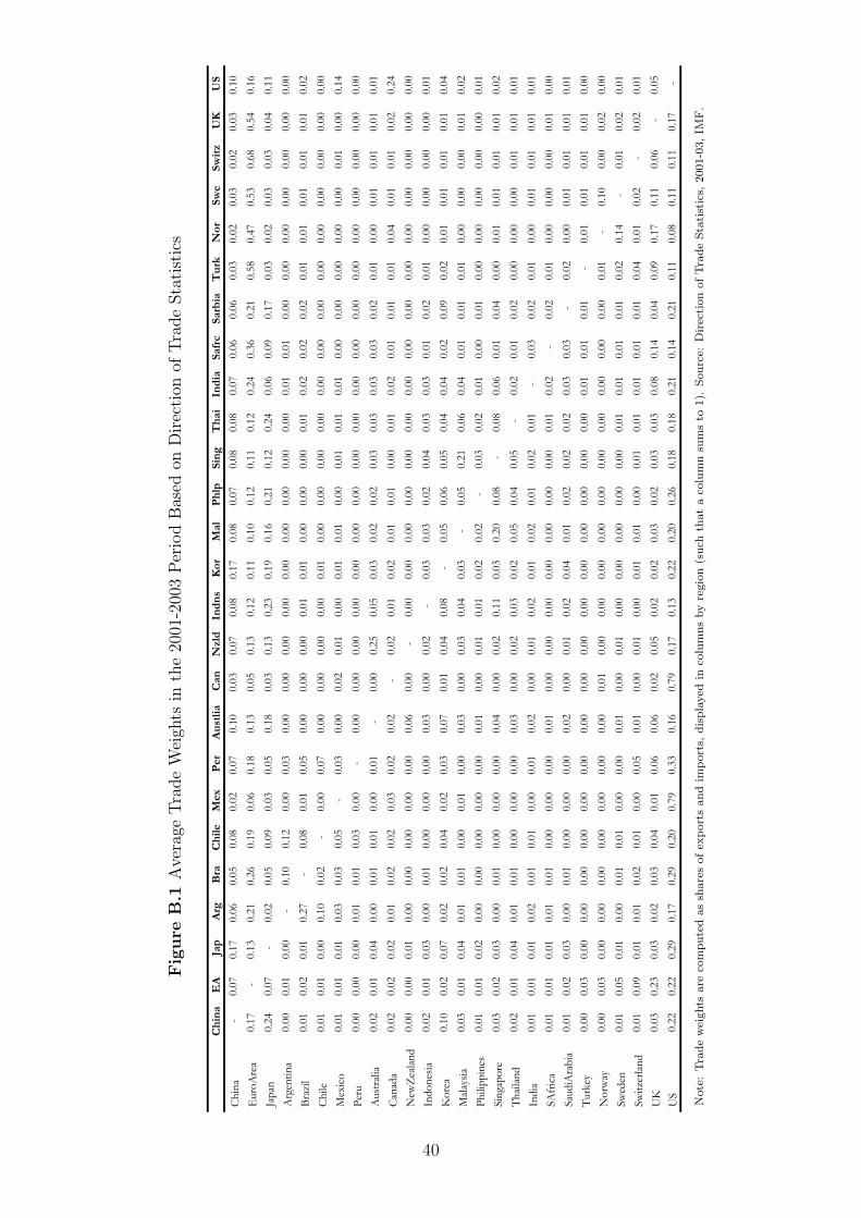
Fig
ure
B.1
Ave
rage
Tra
de
Wei
ghts
inth
e20
01-2
003
Per
iod
Bas
edon
Dir
ecti
onof
Tra
de
Sta
tist
ics
China
EA
Jap
Arg
Bra
Chile
Mex
Per
Austlia
Can
Nzld
Indns
Kor
Mal
Phlp
Sing
Thai
India
SafrcSarbia
Turk
Nor
Swe
Switz
UK
US
China
-0.07
0.17
0.06
0.05
0.08
0.02
0.07
0.10
0.03
0.07
0.08
0.17
0.08
0.07
0.08
0.08
0.07
0.06
0.06
0.03
0.02
0.03
0.02
0.03
0.10
EuroArea
0.17
-0.13
0.21
0.26
0.19
0.06
0.18
0.13
0.05
0.13
0.12
0.11
0.10
0.12
0.11
0.12
0.24
0.36
0.21
0.58
0.47
0.53
0.68
0.54
0.16
Japan
0.24
0.07
-0.02
0.05
0.09
0.03
0.05
0.18
0.03
0.13
0.23
0.19
0.16
0.21
0.12
0.24
0.06
0.09
0.17
0.03
0.02
0.03
0.03
0.04
0.11
Argentina
0.00
0.01
0.00
-0.10
0.12
0.00
0.03
0.00
0.00
0.00
0.00
0.00
0.00
0.00
0.00
0.00
0.01
0.01
0.00
0.00
0.00
0.00
0.00
0.00
0.00
Brazil
0.01
0.02
0.01
0.27
-0.08
0.01
0.05
0.00
0.00
0.00
0.01
0.01
0.00
0.00
0.00
0.01
0.02
0.02
0.02
0.01
0.01
0.01
0.01
0.01
0.02
Chile
0.01
0.01
0.00
0.10
0.02
-0.00
0.07
0.00
0.00
0.00
0.00
0.01
0.00
0.00
0.00
0.00
0.00
0.00
0.00
0.00
0.00
0.00
0.00
0.00
0.00
Mexico
0.01
0.01
0.01
0.03
0.03
0.05
-0.03
0.00
0.02
0.01
0.00
0.01
0.01
0.00
0.01
0.01
0.01
0.00
0.00
0.00
0.00
0.00
0.01
0.00
0.14
Peru
0.00
0.00
0.00
0.01
0.01
0.03
0.00
-0.00
0.00
0.00
0.00
0.00
0.00
0.00
0.00
0.00
0.00
0.00
0.00
0.00
0.00
0.00
0.00
0.00
0.00
Australia
0.02
0.01
0.04
0.00
0.01
0.01
0.00
0.01
-0.00
0.25
0.05
0.03
0.02
0.02
0.03
0.03
0.03
0.03
0.02
0.01
0.00
0.01
0.01
0.01
0.01
Canada
0.02
0.02
0.02
0.01
0.02
0.02
0.03
0.02
0.02
-0.02
0.01
0.02
0.01
0.01
0.00
0.01
0.02
0.01
0.01
0.01
0.04
0.01
0.01
0.02
0.24
NewZealand
0.00
0.00
0.01
0.00
0.00
0.00
0.00
0.00
0.06
0.00
-0.00
0.00
0.00
0.00
0.00
0.00
0.00
0.00
0.00
0.00
0.00
0.00
0.00
0.00
0.00
Indonesia
0.02
0.01
0.03
0.00
0.01
0.00
0.00
0.00
0.03
0.00
0.02
-0.03
0.03
0.02
0.04
0.03
0.03
0.01
0.02
0.01
0.00
0.00
0.00
0.00
0.01
Korea
0.10
0.02
0.07
0.02
0.02
0.04
0.02
0.03
0.07
0.01
0.04
0.08
-0.05
0.06
0.05
0.04
0.04
0.02
0.09
0.02
0.01
0.01
0.01
0.01
0.04
Malaysia
0.03
0.01
0.04
0.01
0.01
0.00
0.01
0.00
0.03
0.00
0.03
0.04
0.03
-0.05
0.21
0.06
0.04
0.01
0.01
0.01
0.00
0.00
0.00
0.01
0.02
Philippines
0.01
0.01
0.02
0.00
0.00
0.00
0.00
0.00
0.01
0.00
0.01
0.01
0.02
0.02
-0.03
0.02
0.01
0.00
0.01
0.00
0.00
0.00
0.00
0.00
0.01
Singapore
0.03
0.02
0.03
0.00
0.01
0.00
0.00
0.00
0.04
0.00
0.02
0.11
0.03
0.20
0.08
-0.08
0.06
0.01
0.04
0.00
0.01
0.01
0.01
0.01
0.02
Thailand
0.02
0.01
0.04
0.01
0.01
0.00
0.00
0.00
0.03
0.00
0.02
0.03
0.02
0.05
0.04
0.05
-0.02
0.01
0.02
0.00
0.00
0.00
0.01
0.01
0.01
India
0.01
0.01
0.01
0.02
0.01
0.01
0.00
0.01
0.02
0.00
0.01
0.02
0.01
0.02
0.01
0.02
0.01
-0.03
0.02
0.01
0.00
0.01
0.01
0.01
0.01
SAfrica
0.01
0.01
0.01
0.01
0.01
0.00
0.00
0.00
0.01
0.00
0.00
0.00
0.00
0.00
0.00
0.00
0.01
0.02
-0.02
0.01
0.00
0.00
0.00
0.01
0.00
SaudiArabia
0.01
0.02
0.03
0.00
0.01
0.00
0.00
0.00
0.02
0.00
0.01
0.02
0.04
0.01
0.02
0.02
0.02
0.03
0.03
-0.02
0.00
0.01
0.01
0.01
0.01
Turkey
0.00
0.03
0.00
0.00
0.00
0.00
0.00
0.00
0.00
0.00
0.00
0.00
0.00
0.00
0.00
0.00
0.00
0.01
0.01
0.01
-0.01
0.01
0.01
0.01
0.00
Norway
0.00
0.03
0.00
0.00
0.00
0.00
0.00
0.00
0.00
0.01
0.00
0.00
0.00
0.00
0.00
0.00
0.00
0.00
0.00
0.00
0.01
-0.10
0.00
0.02
0.00
Sweden
0.01
0.05
0.01
0.00
0.01
0.01
0.00
0.00
0.01
0.00
0.01
0.00
0.00
0.00
0.00
0.00
0.01
0.01
0.01
0.01
0.02
0.14
-0.01
0.02
0.01
Switzerland
0.01
0.09
0.01
0.01
0.02
0.01
0.00
0.05
0.01
0.00
0.01
0.00
0.01
0.01
0.00
0.01
0.01
0.01
0.01
0.01
0.04
0.01
0.02
-0.02
0.01
UK
0.03
0.23
0.03
0.02
0.03
0.04
0.01
0.06
0.06
0.02
0.05
0.02
0.02
0.03
0.02
0.03
0.03
0.08
0.14
0.04
0.09
0.17
0.11
0.06
-0.05
US
0.22
0.22
0.29
0.17
0.29
0.20
0.79
0.33
0.16
0.79
0.17
0.13
0.22
0.20
0.26
0.18
0.18
0.21
0.14
0.21
0.11
0.08
0.11
0.11
0.17
-
Note
:Tra
de
wei
ghts
are
com
pute
das
share
sofex
port
sand
import
s,dis
pla
yed
inco
lum
ns
by
regio
n(s
uch
that
aco
lum
nsu
ms
to1).
Sourc
e:D
irec
tion
ofTra
de
Sta
tist
ics,
2001-0
3,IM
F.
40
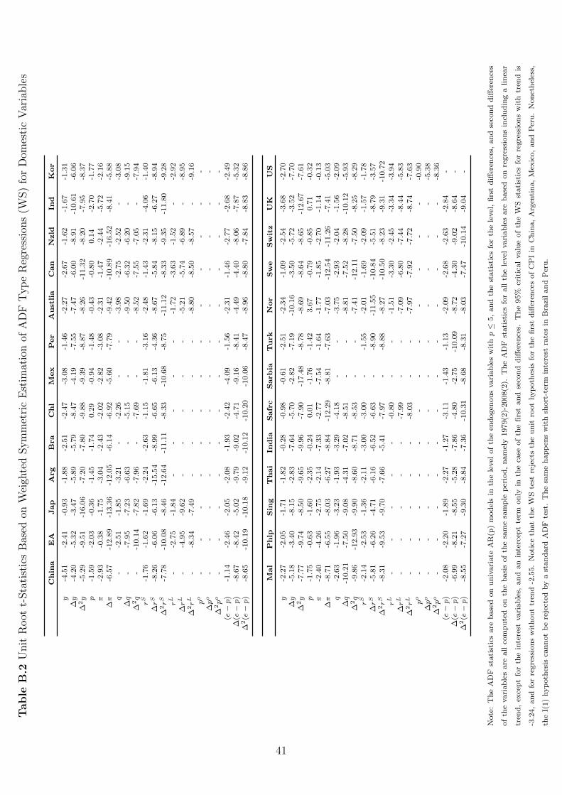
Table
B.2
Unit
Root
t-Sta
tist
ics
Bas
edon
Wei
ghte
dSym
met
ric
Est
imat
ion
ofA
DF
Type
Reg
ress
ions
(WS)
for
Dom
esti
cV
aria
ble
s
Chin
aEA
Jap
Arg
Bra
Chl
Mex
Per
Aust
lia
Can
Nzld
Ind
Kor
y-4
.51
-2.4
1-0
.93
-1.8
8-2
.51
-2.4
7-3
.08
-1.4
6-2
.27
-2.6
7-1
.62
-1.6
7-1
.31
∆y
-4.2
0-5
.32
-3.4
7-5
.89
-5.7
9-8
.47
-4.1
9-7
.55
-7.4
7-6
.00
-8.9
1-1
0.6
1-6
.06
∆2y
-5.2
9-9
.51
-16.0
6-7
.20
-7.8
0-9
.88
-9.3
9-8
.87
-8.2
6-1
1.3
2-8
.20
-7.9
5-8
.37
p-1
.59
-2.0
3-0
.36
-1.4
5-1
.74
0.2
9-0
.94
-1.4
8-0
.43
-0.8
00.1
4-2
.70
-1.7
7π
-2.9
3-0
.38
-1.7
5-3
.04
-2.4
3-2
.02
-2.8
2-3
.08
-2.3
1-1
.47
-2.4
4-5
.72
-2.1
6∆
π-6
.57
-12.8
9-1
3.3
6-1
2.0
5-6
.14
-6.9
2-5
.60
-7.7
9-9
.42
-10.8
9-1
6.5
2-8
.41
-5.8
8q
--2
.51
-1.8
5-3
.21
--2
.26
--
-3.9
8-2
.75
-2.5
2-
-3.0
8∆
q-
-7.9
5-7
.23
-6.6
3-
-5.1
5-
--9
.50
-6.3
2-6
.20
--9
.15
∆2q
--1
0.1
4-7
.82
-7.9
6-
-7.6
9-
--8
.52
-7.5
5-7
.05
--7
.94
rS
-1.7
6-1
.62
-1.6
9-2
.24
-2.6
3-1
.15
-1.8
1-3
.16
-2.4
8-1
.43
-2.3
1-4
.06
-1.4
0∆
rS
-8.2
6-6
.06
-6.1
3-1
5.5
4-8
.99
-6.6
5-6
.13
-4.3
6-8
.67
-5.8
4-8
.15
-6.2
7-8
.94
∆2r
S-7
.78
-10.0
8-8
.46
-12.6
4-1
1.1
1-8
.33
-10.6
8-8
.75
-11.1
2-8
.33
-9.3
5-1
1.8
0-9
.28
rL
--2
.75
-1.8
4-
--
--
-1.7
2-3
.63
-1.5
2-
-2.9
2∆
rL
--4
.95
-9.6
2-
--
--
-5.2
1-5
.74
-6.8
9-
-8.9
5∆
2r
L-
-8.3
4-7
.49
--
--
--8
.80
-8.5
0-8
.57
--9
.16
po
--
--
--
--
--
--
-∆
po
--
--
--
--
--
--
-∆
2p
o-
--
--
--
--
--
--
(e−
p)
-1.1
4-2
.46
-2.0
5-2
.08
-1.9
3-2
.42
-4.0
9-1
.56
-2.3
1-1
.46
-2.7
7-2
.68
-2.4
9∆
(e−
p)
-8.6
7-8
.42
-5.0
2-9
.79
-9.0
2-4
.71
-9.1
6-8
.41
-4.4
9-4
.40
-8.0
6-7
.87
-5.3
2∆
2(e−
p)
-8.6
5-1
0.1
9-1
0.1
8-9
.12
-10.1
2-1
0.2
0-1
0.0
6-8
.47
-8.9
6-8
.80
-7.8
4-8
.83
-8.8
6
Mal
Phlp
Sin
gT
hai
India
Safr
cSarbia
Turk
Nor
Sw
eSw
itz
UK
US
y-2
.27
-2.0
5-1
.71
-1.8
2-0
.28
-0.9
8-0
.61
-2.5
1-2
.34
-1.0
9-2
.54
-3.6
8-2
.70
∆y
-5.1
8-3
.40
-8.1
5-2
.83
-7.6
4-5
.70
-2.8
2-7
.19
-10.1
6-3
.50
-5.7
2-3
.52
-7.7
0∆
2y
-7.7
7-9
.74
-8.5
0-9
.65
-9.9
6-7
.90
-17.4
8-8
.78
-8.6
9-8
.64
-8.6
5-1
2.6
7-7
.61
p-1
.75
-0.6
3-1
.60
-2.3
5-0
.24
0.0
1-1
.76
-1.4
23.6
7-0
.79
-0.8
50.7
1-0
.32
π-2
.40
-4.2
6-2
.75
-2.1
4-7
.33
-2.7
7-7
.54
-1.6
4-1
.77
-1.8
5-2
.70
-1.1
4-0
.13
∆π
-8.7
1-6
.55
-8.0
3-6
.27
-8.8
4-1
2.2
9-8
.81
-7.6
3-7
.03
-12.5
4-1
1.2
6-7
.41
-5.0
3q
-2.6
3-1
.96
-3.2
3-1
.93
-3.2
9-4
.18
--
-3.7
5-2
.93
-2.0
4-1
.56
-2.0
9∆
q-1
0.2
1-7
.50
-9.0
8-4
.31
-7.0
2-8
.51
--
-8.8
1-7
.52
-8.2
8-1
0.1
2-5
.93
∆2q
-9.8
6-1
2.9
3-9
.90
-8.6
0-8
.71
-8.5
3-
--7
.41
-12.1
1-7
.50
-8.2
5-8
.29
rS
-2.1
4-2
.53
-1.3
6-2
.11
-3.0
0-3
.00
--1
.55
-2.0
1-1
.69
-2.0
9-1
.57
-1.7
8∆
rS
-5.8
1-6
.26
-4.7
1-6
.16
-6.5
2-6
.63
--8
.90
-11.5
5-1
0.8
4-5
.51
-8.7
9-3
.57
∆2r
S-8
.31
-9.5
3-9
.70
-7.6
6-5
.41
-7.9
7-
-8.8
8-8
.27
-10.5
0-8
.23
-9.3
1-1
0.7
2r
L-
--
--
-0.8
0-
--1
.51
-3.3
0-2
.45
-3.3
4-3
.94
∆r
L-
--
--
-7.9
9-
--7
.09
-6.8
0-7
.44
-8.4
4-5
.83
∆2r
L-
--
--
-8.0
3-
--7
.97
-7.9
2-7
.72
-8.7
4-7
.63
po
--
--
--
--
--
--
-0.9
0∆
po
--
--
--
--
--
--
-5.3
8∆
2p
o-
--
--
--
--
--
--8
.36
(e−
p)
-2.0
8-2
.20
-1.8
9-2
.27
-1.2
7-3
.11
-1.4
3-1
.13
-2.0
9-2
.68
-2.6
3-2
.84
-∆
(e−
p)
-6.9
9-8
.21
-8.5
5-5
.28
-7.8
6-4
.80
-2.7
5-1
0.0
9-8
.72
-4.3
0-9
.02
-8.6
4-
∆2(e−
p)
-8.5
5-7
.27
-9.3
0-8
.84
-7.3
6-1
0.3
1-8
.68
-8.3
1-8
.03
-7.4
7-1
0.1
4-9
.04
-
Note
:T
he
AD
Fst
atist
ics
are
base
don
univ
ari
ate
AR
(p)
model
sin
the
level
ofth
een
dogen
ous
vari
able
sw
ith
p≤
5,and
the
stati
stic
sfo
rth
ele
vel
,firs
tdiff
eren
ces,
and
seco
nd
diff
eren
ces
ofth
evari
able
sare
all
com
pute
don
the
basi
softh
esa
me
sam
ple
per
iod,nam
ely
1979(2
)-2008(2
).T
he
AD
Fst
ati
stic
sfo
rall
the
level
vari
able
sare
base
don
regre
ssio
ns
incl
udin
ga
linea
r
tren
d,ex
cept
for
the
inte
rest
vari
able
s,and
an
inte
rcep
tte
rmonly
inth
eca
seof
the
firs
tand
seco
nd
diff
eren
ces.
The
95%
critic
alvalu
eof
the
WS
stati
stic
sfo
rre
gre
ssio
ns
with
tren
dis
-3.2
4,and
for
regre
ssio
ns
without
tren
d-2
.55.
Notice
that
the
WS
test
reje
cts
the
unit
root
hypoth
esis
for
the
firs
tdiff
eren
ces
ofC
PI
inC
hin
a,A
rgen
tina,M
exic
o,and
Per
u.
Nonet
hel
ess,
the
I(1)
hypoth
esis
cannot
be
reje
cted
by
ast
andard
AD
Fte
st.
The
sam
ehappen
sw
ith
short
-ter
min
tere
stra
tes
inB
razi
land
Per
u.
41
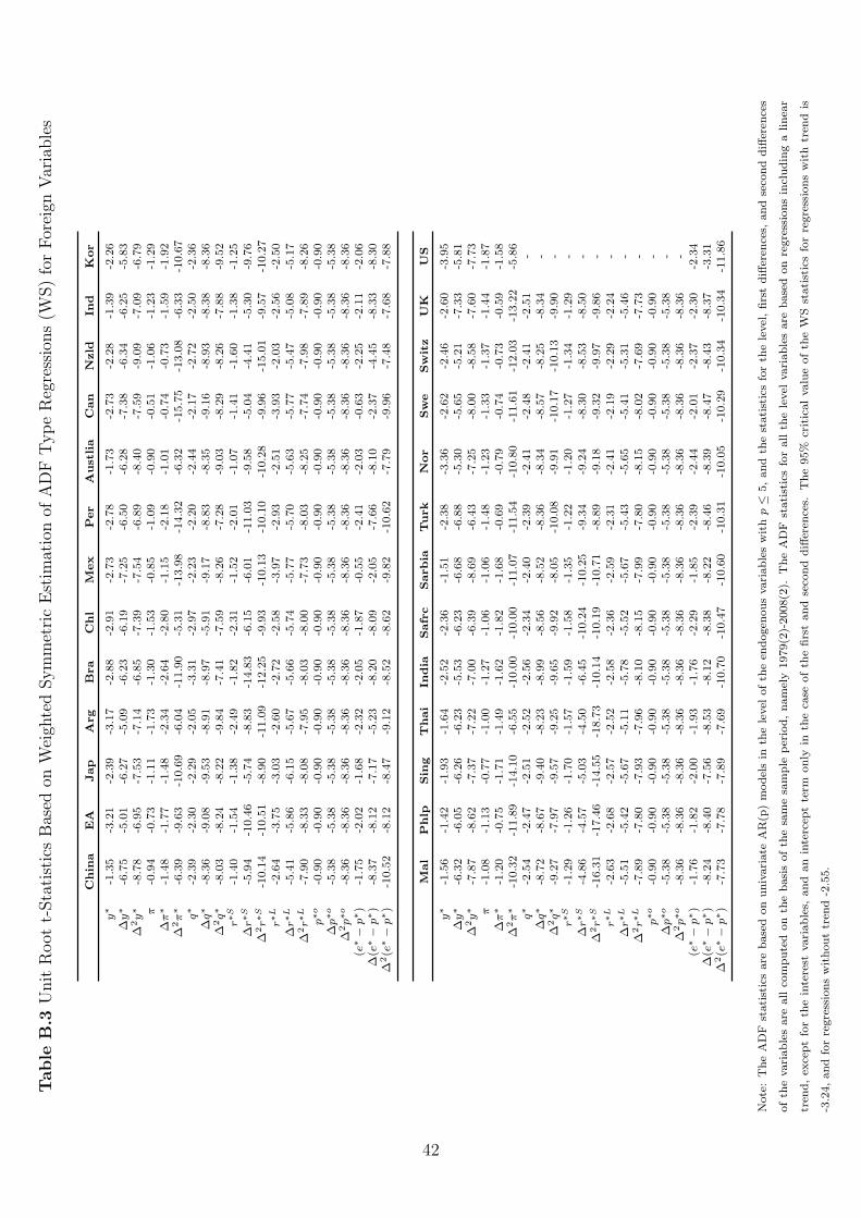
Table
B.3
Unit
Root
t-Sta
tist
ics
Bas
edon
Wei
ghte
dSym
met
ric
Est
imat
ion
ofA
DF
Type
Reg
ress
ions
(WS)
for
For
eign
Var
iable
s
Chin
aEA
Jap
Arg
Bra
Chl
Mex
Per
Aust
lia
Can
Nzld
Ind
Kor
y∗
-1.3
5-3
.21
-2.3
9-3
.17
-2.8
8-2
.91
-2.7
3-2
.78
-1.7
3-2
.73
-2.2
8-1
.39
-2.2
6∆
y∗
-6.7
5-5
.01
-6.2
7-5
.09
-6.2
3-6
.19
-7.2
5-6
.50
-6.2
8-7
.38
-6.3
4-6
.25
-5.8
3∆
2y∗
-8.7
8-6
.95
-7.5
3-7
.14
-6.8
5-7
.39
-7.5
4-6
.89
-8.4
0-7
.59
-9.0
9-7
.09
-6.7
9π
-0.9
4-0
.73
-1.1
1-1
.73
-1.3
0-1
.53
-0.8
5-1
.09
-0.9
0-0
.51
-1.0
6-1
.23
-1.2
9∆
π∗
-1.4
8-1
.77
-1.4
8-2
.34
-2.6
4-2
.80
-1.1
5-2
.18
-1.0
1-0
.74
-0.7
3-1
.59
-1.9
2∆
2π∗
-6.3
9-9
.63
-10.6
9-6
.04
-11.9
0-5
.31
-13.9
8-1
4.3
2-6
.32
-15.7
5-1
3.0
8-6
.33
-10.6
7q∗
-2.3
9-2
.30
-2.2
9-2
.05
-3.3
1-2
.97
-2.2
3-2
.20
-2.4
4-2
.17
-2.7
2-2
.50
-2.3
6∆
q∗
-8.3
6-9
.08
-9.5
3-8
.91
-8.9
7-5
.91
-9.1
7-8
.83
-8.3
5-9
.16
-8.9
3-8
.38
-8.3
6∆
2q∗
-8.0
3-8
.24
-8.2
2-9
.84
-7.4
1-7
.59
-8.2
6-7
.28
-9.0
3-8
.29
-8.2
6-7
.88
-9.5
2r∗S
-1.4
0-1
.54
-1.3
8-2
.49
-1.8
2-2
.31
-1.5
2-2
.01
-1.0
7-1
.41
-1.6
0-1
.38
-1.2
5∆
r∗S
-5.9
4-1
0.4
6-5
.74
-8.8
3-1
4.8
3-6
.15
-6.0
1-1
1.0
3-9
.58
-5.0
4-4
.41
-5.3
0-9
.76
∆2r∗S
-10.1
4-1
0.5
1-8
.90
-11.0
9-1
2.2
5-9
.93
-10.1
3-1
0.1
0-1
0.2
8-9
.96
-15.0
1-9
.57
-10.2
7r∗L
-2.6
4-3
.75
-3.0
3-2
.60
-2.7
2-2
.58
-3.9
7-2
.93
-2.5
1-3
.93
-2.0
3-2
.56
-2.5
0∆
r∗L
-5.4
1-5
.86
-6.1
5-5
.67
-5.6
6-5
.74
-5.7
7-5
.70
-5.6
3-5
.77
-5.4
7-5
.08
-5.1
7∆
2r∗L
-7.9
0-8
.33
-8.0
8-7
.95
-8.0
3-8
.00
-7.7
3-8
.03
-8.2
5-7
.74
-7.9
8-7
.89
-8.2
6p∗o
-0.9
0-0
.90
-0.9
0-0
.90
-0.9
0-0
.90
-0.9
0-0
.90
-0.9
0-0
.90
-0.9
0-0
.90
-0.9
0∆
p∗o
-5.3
8-5
.38
-5.3
8-5
.38
-5.3
8-5
.38
-5.3
8-5
.38
-5.3
8-5
.38
-5.3
8-5
.38
-5.3
8∆
2p∗o
-8.3
6-8
.36
-8.3
6-8
.36
-8.3
6-8
.36
-8.3
6-8
.36
-8.3
6-8
.36
-8.3
6-8
.36
-8.3
6(e
∗−
p∗)
-1.7
5-2
.02
-1.6
8-2
.32
-2.0
5-1
.87
-0.5
5-2
.41
-2.0
3-0
.63
-2.2
5-2
.11
-2.0
6∆
(e∗−
p∗)
-8.3
7-8
.12
-7.1
7-5
.23
-8.2
0-8
.09
-2.0
5-7
.66
-8.1
0-2
.37
-4.4
5-8
.33
-8.3
0∆
2(e
∗−
p∗)
-10.5
2-8
.12
-8.4
7-9
.12
-8.5
2-8
.62
-9.8
2-1
0.6
2-7
.79
-9.9
6-7
.48
-7.6
8-7
.88
Mal
Phlp
Sin
gT
hai
India
Safr
cSarbia
Turk
Nor
Sw
eSw
itz
UK
US
y∗
-1.5
6-1
.42
-1.9
3-1
.64
-2.5
2-2
.36
-1.5
1-2
.38
-3.3
6-2
.62
-2.4
6-2
.60
-3.9
5∆
y∗
-6.3
2-6
.05
-6.2
6-6
.23
-5.5
3-6
.23
-6.6
8-6
.88
-5.3
0-5
.65
-5.2
1-7
.33
-5.8
1∆
2y∗
-7.8
7-8
.62
-7.3
7-7
.22
-7.0
0-6
.39
-8.6
9-6
.43
-7.2
5-8
.00
-8.5
8-7
.60
-7.7
3π
-1.0
8-1
.13
-0.7
7-1
.00
-1.2
7-1
.06
-1.0
6-1
.48
-1.2
3-1
.33
-1.3
7-1
.44
-1.8
7∆
π∗
-1.2
0-0
.75
-1.7
1-1
.49
-1.6
2-1
.82
-1.6
8-0
.69
-0.7
9-0
.74
-0.7
3-0
.59
-1.5
8∆
2π∗
-10.3
2-1
1.8
9-1
4.1
0-6
.55
-10.0
0-1
0.0
0-1
1.0
7-1
1.5
4-1
0.8
0-1
1.6
1-1
2.0
3-1
3.2
2-5
.86
q∗
-2.5
4-2
.47
-2.5
1-2
.52
-2.5
6-2
.34
-2.4
0-2
.39
-2.4
1-2
.48
-2.4
1-2
.51
-∆
q∗
-8.7
2-8
.67
-9.4
0-8
.23
-8.9
9-8
.56
-8.5
2-8
.36
-8.3
4-8
.57
-8.2
5-8
.34
-∆
2q∗
-9.2
7-7
.97
-9.5
7-9
.25
-9.6
5-9
.92
-8.0
5-1
0.0
8-9
.91
-10.1
7-1
0.1
3-9
.90
-r∗S
-1.2
9-1
.26
-1.7
0-1
.57
-1.5
9-1
.58
-1.3
5-1
.22
-1.2
0-1
.27
-1.3
4-1
.29
-∆
r∗S
-4.8
6-4
.57
-5.0
3-4
.50
-6.4
5-1
0.2
4-1
0.2
5-9
.34
-9.2
4-8
.30
-8.5
3-8
.50
-∆
2r∗S
-16.3
1-1
7.4
6-1
4.5
5-1
8.7
3-1
0.1
4-1
0.1
9-1
0.7
1-8
.89
-9.1
8-9
.32
-9.9
7-9
.86
-r∗L
-2.6
3-2
.68
-2.5
7-2
.52
-2.5
8-2
.36
-2.5
9-2
.31
-2.4
1-2
.19
-2.2
9-2
.24
-∆
r∗L
-5.5
1-5
.42
-5.6
7-5
.11
-5.7
8-5
.52
-5.6
7-5
.43
-5.6
5-5
.41
-5.3
1-5
.46
-∆
2r∗L
-7.8
9-7
.80
-7.9
3-7
.96
-8.1
0-8
.15
-7.9
9-7
.80
-8.1
5-8
.02
-7.6
9-7
.73
-p∗o
-0.9
0-0
.90
-0.9
0-0
.90
-0.9
0-0
.90
-0.9
0-0
.90
-0.9
0-0
.90
-0.9
0-0
.90
-∆
p∗o
-5.3
8-5
.38
-5.3
8-5
.38
-5.3
8-5
.38
-5.3
8-5
.38
-5.3
8-5
.38
-5.3
8-5
.38
-∆
2p∗o
-8.3
6-8
.36
-8.3
6-8
.36
-8.3
6-8
.36
-8.3
6-8
.36
-8.3
6-8
.36
-8.3
6-8
.36
-(e
∗−
p∗)
-1.7
6-1
.82
-2.0
0-1
.93
-1.7
6-2
.29
-1.8
5-2
.39
-2.4
4-2
.01
-2.3
7-2
.30
-2.3
4∆
(e∗−
p∗)
-8.2
4-8
.40
-7.5
6-8
.53
-8.1
2-8
.38
-8.2
2-8
.46
-8.3
9-8
.47
-8.4
3-8
.37
-3.3
1∆
2(e
∗−
p∗)
-7.7
3-7
.78
-7.8
9-7
.69
-10.7
0-1
0.4
7-1
0.6
0-1
0.3
1-1
0.0
5-1
0.2
9-1
0.3
4-1
0.3
4-1
1.8
6
Note
:T
he
AD
Fst
atist
ics
are
base
don
univ
ari
ate
AR
(p)
model
sin
the
level
ofth
een
dogen
ous
vari
able
sw
ith
p≤
5,and
the
stati
stic
sfo
rth
ele
vel
,firs
tdiff
eren
ces,
and
seco
nd
diff
eren
ces
ofth
evari
able
sare
all
com
pute
don
the
basi
softh
esa
me
sam
ple
per
iod,nam
ely
1979(2
)-2008(2
).T
he
AD
Fst
ati
stic
sfo
rall
the
level
vari
able
sare
base
don
regre
ssio
ns
incl
udin
ga
linea
r
tren
d,ex
cept
for
the
inte
rest
vari
able
s,and
an
inte
rcep
tte
rmonly
inth
eca
seof
the
firs
tand
seco
nd
diff
eren
ces.
The
95%
critic
alvalu
eof
the
WS
stati
stic
sfo
rre
gre
ssio
ns
with
tren
dis
-3.2
4,and
for
regre
ssio
ns
without
tren
d-2
.55.
42
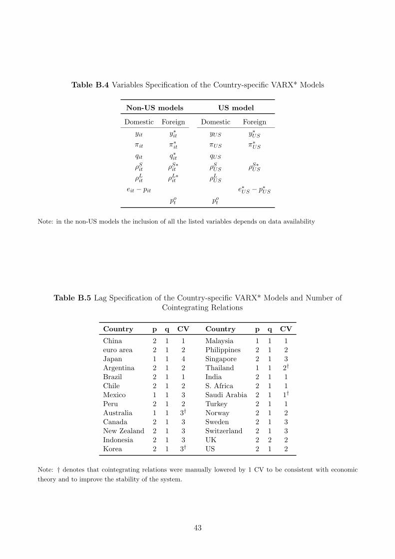
Table B.4 Variables Specification of the Country-specific VARX* Models
Non-US models US model
Domestic Foreign Domestic Foreign
yit y∗it yUS y∗US
πit π∗it πUS π∗US
qit q∗it qUS
ρSit ρS∗
it ρSUS ρS∗
US
ρLit ρL∗
it ρLUS
eit − pit e∗US − p∗US
pot po
t
Note: in the non-US models the inclusion of all the listed variables depends on data availability
Table B.5 Lag Specification of the Country-specific VARX* Models and Number ofCointegrating Relations
Country p q CV Country p q CV
China 2 1 1 Malaysia 1 1 1euro area 2 1 2 Philippines 2 1 2Japan 1 1 4 Singapore 2 1 3Argentina 2 1 2 Thailand 1 1 2†
Brazil 2 1 1 India 2 1 1Chile 2 1 2 S. Africa 2 1 1Mexico 1 1 3 Saudi Arabia 2 1 1†
Peru 2 1 2 Turkey 2 1 1Australia 1 1 3† Norway 2 1 2Canada 2 1 3 Sweden 2 1 3New Zealand 2 1 3 Switzerland 2 1 3Indonesia 2 1 3 UK 2 2 2Korea 2 1 3† US 2 1 2
Note: † denotes that cointegrating relations were manually lowered by 1 CV to be consistent with economictheory and to improve the stability of the system.
43
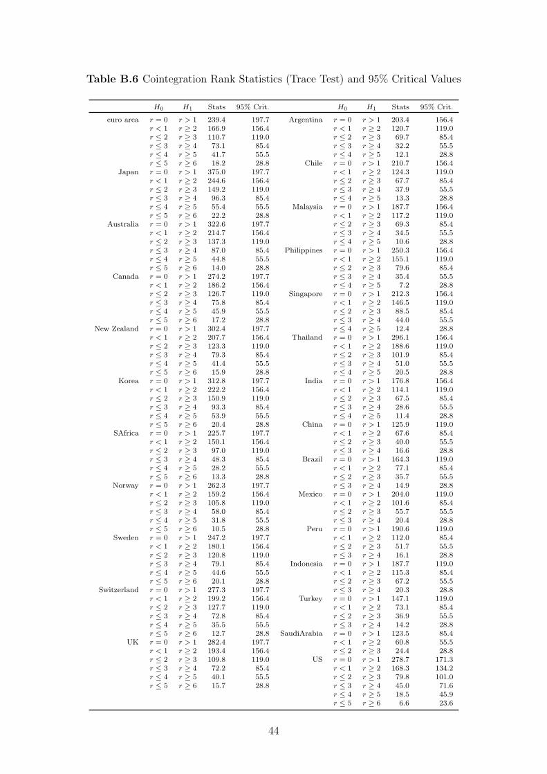
Table B.6 Cointegration Rank Statistics (Trace Test) and 95% Critical Values
H0 H1 Stats 95% Crit. H0 H1 Stats 95% Crit.
euro area r = 0 r > 1 239.4 197.7 Argentina r = 0 r > 1 203.4 156.4r < 1 r ≥ 2 166.9 156.4 r < 1 r ≥ 2 120.7 119.0r ≤ 2 r ≥ 3 110.7 119.0 r ≤ 2 r ≥ 3 69.7 85.4r ≤ 3 r ≥ 4 73.1 85.4 r ≤ 3 r ≥ 4 32.2 55.5r ≤ 4 r ≥ 5 41.7 55.5 r ≤ 4 r ≥ 5 12.1 28.8r ≤ 5 r ≥ 6 18.2 28.8 Chile r = 0 r > 1 210.7 156.4
Japan r = 0 r > 1 375.0 197.7 r < 1 r ≥ 2 124.3 119.0r < 1 r ≥ 2 244.6 156.4 r ≤ 2 r ≥ 3 67.7 85.4r ≤ 2 r ≥ 3 149.2 119.0 r ≤ 3 r ≥ 4 37.9 55.5r ≤ 3 r ≥ 4 96.3 85.4 r ≤ 4 r ≥ 5 13.3 28.8r ≤ 4 r ≥ 5 55.4 55.5 Malaysia r = 0 r > 1 187.7 156.4r ≤ 5 r ≥ 6 22.2 28.8 r < 1 r ≥ 2 117.2 119.0
Australia r = 0 r > 1 322.6 197.7 r ≤ 2 r ≥ 3 69.3 85.4r < 1 r ≥ 2 214.7 156.4 r ≤ 3 r ≥ 4 34.5 55.5r ≤ 2 r ≥ 3 137.3 119.0 r ≤ 4 r ≥ 5 10.6 28.8r ≤ 3 r ≥ 4 87.0 85.4 Philippines r = 0 r > 1 250.3 156.4r ≤ 4 r ≥ 5 44.8 55.5 r < 1 r ≥ 2 155.1 119.0r ≤ 5 r ≥ 6 14.0 28.8 r ≤ 2 r ≥ 3 79.6 85.4
Canada r = 0 r > 1 274.2 197.7 r ≤ 3 r ≥ 4 35.4 55.5r < 1 r ≥ 2 186.2 156.4 r ≤ 4 r ≥ 5 7.2 28.8r ≤ 2 r ≥ 3 126.7 119.0 Singapore r = 0 r > 1 212.3 156.4r ≤ 3 r ≥ 4 75.8 85.4 r < 1 r ≥ 2 146.5 119.0r ≤ 4 r ≥ 5 45.9 55.5 r ≤ 2 r ≥ 3 88.5 85.4r ≤ 5 r ≥ 6 17.2 28.8 r ≤ 3 r ≥ 4 44.0 55.5
New Zealand r = 0 r > 1 302.4 197.7 r ≤ 4 r ≥ 5 12.4 28.8r < 1 r ≥ 2 207.7 156.4 Thailand r = 0 r > 1 296.1 156.4r ≤ 2 r ≥ 3 123.3 119.0 r < 1 r ≥ 2 188.6 119.0r ≤ 3 r ≥ 4 79.3 85.4 r ≤ 2 r ≥ 3 101.9 85.4r ≤ 4 r ≥ 5 41.4 55.5 r ≤ 3 r ≥ 4 51.0 55.5r ≤ 5 r ≥ 6 15.9 28.8 r ≤ 4 r ≥ 5 20.5 28.8
Korea r = 0 r > 1 312.8 197.7 India r = 0 r > 1 176.8 156.4r < 1 r ≥ 2 222.2 156.4 r < 1 r ≥ 2 114.1 119.0r ≤ 2 r ≥ 3 150.9 119.0 r ≤ 2 r ≥ 3 67.5 85.4r ≤ 3 r ≥ 4 93.3 85.4 r ≤ 3 r ≥ 4 28.6 55.5r ≤ 4 r ≥ 5 53.9 55.5 r ≤ 4 r ≥ 5 11.4 28.8r ≤ 5 r ≥ 6 20.4 28.8 China r = 0 r > 1 125.9 119.0
SAfrica r = 0 r > 1 225.7 197.7 r < 1 r ≥ 2 67.6 85.4r < 1 r ≥ 2 150.1 156.4 r ≤ 2 r ≥ 3 40.0 55.5r ≤ 2 r ≥ 3 97.0 119.0 r ≤ 3 r ≥ 4 16.6 28.8r ≤ 3 r ≥ 4 48.3 85.4 Brazil r = 0 r > 1 164.3 119.0r ≤ 4 r ≥ 5 28.2 55.5 r < 1 r ≥ 2 77.1 85.4r ≤ 5 r ≥ 6 13.3 28.8 r ≤ 2 r ≥ 3 35.7 55.5
Norway r = 0 r > 1 262.3 197.7 r ≤ 3 r ≥ 4 14.9 28.8r < 1 r ≥ 2 159.2 156.4 Mexico r = 0 r > 1 204.0 119.0r ≤ 2 r ≥ 3 105.8 119.0 r < 1 r ≥ 2 101.6 85.4r ≤ 3 r ≥ 4 58.0 85.4 r ≤ 2 r ≥ 3 55.7 55.5r ≤ 4 r ≥ 5 31.8 55.5 r ≤ 3 r ≥ 4 20.4 28.8r ≤ 5 r ≥ 6 10.5 28.8 Peru r = 0 r > 1 190.6 119.0
Sweden r = 0 r > 1 247.2 197.7 r < 1 r ≥ 2 112.0 85.4r < 1 r ≥ 2 180.1 156.4 r ≤ 2 r ≥ 3 51.7 55.5r ≤ 2 r ≥ 3 120.8 119.0 r ≤ 3 r ≥ 4 16.1 28.8r ≤ 3 r ≥ 4 79.1 85.4 Indonesia r = 0 r > 1 187.7 119.0r ≤ 4 r ≥ 5 44.6 55.5 r < 1 r ≥ 2 115.3 85.4r ≤ 5 r ≥ 6 20.1 28.8 r ≤ 2 r ≥ 3 67.2 55.5
Switzerland r = 0 r > 1 277.3 197.7 r ≤ 3 r ≥ 4 20.3 28.8r < 1 r ≥ 2 199.2 156.4 Turkey r = 0 r > 1 147.1 119.0r ≤ 2 r ≥ 3 127.7 119.0 r < 1 r ≥ 2 73.1 85.4r ≤ 3 r ≥ 4 72.8 85.4 r ≤ 2 r ≥ 3 36.9 55.5r ≤ 4 r ≥ 5 35.5 55.5 r ≤ 3 r ≥ 4 14.2 28.8r ≤ 5 r ≥ 6 12.7 28.8 SaudiArabia r = 0 r > 1 123.5 85.4
UK r = 0 r > 1 282.4 197.7 r < 1 r ≥ 2 60.8 55.5r < 1 r ≥ 2 193.4 156.4 r ≤ 2 r ≥ 3 24.4 28.8r ≤ 2 r ≥ 3 109.8 119.0 US r = 0 r > 1 278.7 171.3r ≤ 3 r ≥ 4 72.2 85.4 r < 1 r ≥ 2 168.3 134.2r ≤ 4 r ≥ 5 40.1 55.5 r ≤ 2 r ≥ 3 79.8 101.0r ≤ 5 r ≥ 6 15.7 28.8 r ≤ 3 r ≥ 4 45.0 71.6
r ≤ 4 r ≥ 5 18.5 45.9r ≤ 5 r ≥ 6 6.6 23.6
44
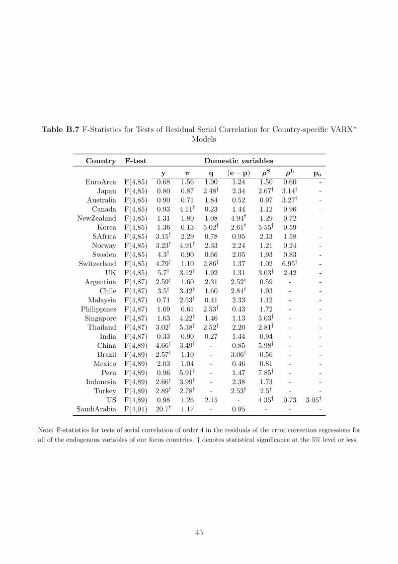
Table B.7 F-Statistics for Tests of Residual Serial Correlation for Country-specific VARX*Models
Country F-test Domestic variables
y π q (e− p) ρS ρL po
EuroArea F(4,85) 0.68 1.56 1.90 1.24 1.50 0.60 -Japan F(4,85) 0.80 0.87 2.48† 2.34 2.67† 3.14† -
Australia F(4,85) 0.90 0.71 1.84 0.52 0.97 3.27† -Canada F(4,85) 0.93 4.11† 0.23 1.44 1.12 0.96 -
NewZealand F(4,85) 1.31 1.80 1.08 4.94† 1.29 0.72 -Korea F(4,85) 1.36 0.13 5.02† 2.61† 5.55† 0.59 -
SAfrica F(4,85) 3.15† 2.29 0.78 0.95 2.13 1.58 -Norway F(4,85) 3.23† 4.91† 2.33 2.24 1.21 0.24 -Sweden F(4,85) 4.3† 0.90 0.66 2.05 1.93 0.83 -
Switzerland F(4,85) 4.79† 1.10 2.86† 1.37 1.02 6.95† -UK F(4,85) 5.7† 3.12† 1.92 1.31 3.03† 2.42 -
Argentina F(4,87) 2.59† 1.60 2.31 2.52† 0.59 - -Chile F(4,87) 3.5† 3.42† 1.60 2.84† 1.93 - -
Malaysia F(4,87) 0.71 2.53† 0.41 2.33 1.12 - -Philippines F(4,87) 1.69 0.61 2.53† 0.43 1.72 - -Singapore F(4,87) 1.63 4.22† 1.46 1.13 3.03† - -Thailand F(4,87) 3.02† 5.38† 2.52† 2.20 2.81† - -
India F(4,87) 0.33 0.90 0.27 1.44 0.94 - -China F(4,89) 4.66† 3.49† - 0.85 5.98† - -Brazil F(4,89) 2.57† 1.10 - 3.06† 0.56 - -
Mexico F(4,89) 2.03 1.04 - 0.46 0.81 - -Peru F(4,89) 0.96 5.91† - 1.47 7.85† - -
Indonesia F(4,89) 2.66† 3.99† - 2.38 1.73 - -Turkey F(4,89) 2.89† 2.78† - 2.53† 2.5† - -
US F(4,89) 0.98 1.26 2.15 - 4.35† 0.73 3.05†
SaudiArabia F(4,91) 20.7† 1.17 - 0.95 - - -
Note: F-statistics for tests of serial correlation of order 4 in the residuals of the error correction regressions forall of the endogenous variables of our focus countries. † denotes statistical significance at the 5% level or less.
45
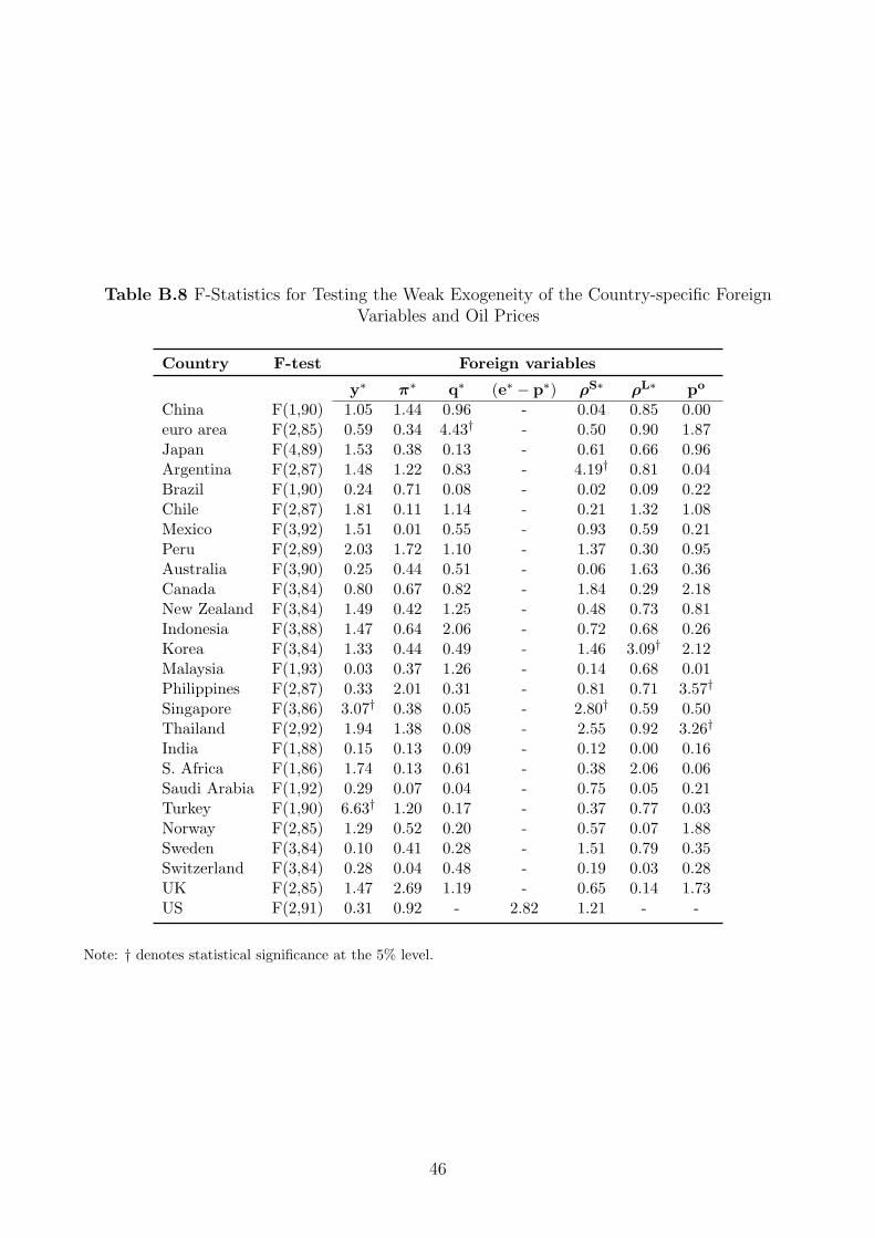
Table B.8 F-Statistics for Testing the Weak Exogeneity of the Country-specific ForeignVariables and Oil Prices
Country F-test Foreign variables
y∗ π∗ q∗ (e∗ − p∗) ρS∗ ρL∗ po
China F(1,90) 1.05 1.44 0.96 - 0.04 0.85 0.00euro area F(2,85) 0.59 0.34 4.43† - 0.50 0.90 1.87Japan F(4,89) 1.53 0.38 0.13 - 0.61 0.66 0.96Argentina F(2,87) 1.48 1.22 0.83 - 4.19† 0.81 0.04Brazil F(1,90) 0.24 0.71 0.08 - 0.02 0.09 0.22Chile F(2,87) 1.81 0.11 1.14 - 0.21 1.32 1.08Mexico F(3,92) 1.51 0.01 0.55 - 0.93 0.59 0.21Peru F(2,89) 2.03 1.72 1.10 - 1.37 0.30 0.95Australia F(3,90) 0.25 0.44 0.51 - 0.06 1.63 0.36Canada F(3,84) 0.80 0.67 0.82 - 1.84 0.29 2.18New Zealand F(3,84) 1.49 0.42 1.25 - 0.48 0.73 0.81Indonesia F(3,88) 1.47 0.64 2.06 - 0.72 0.68 0.26Korea F(3,84) 1.33 0.44 0.49 - 1.46 3.09† 2.12Malaysia F(1,93) 0.03 0.37 1.26 - 0.14 0.68 0.01Philippines F(2,87) 0.33 2.01 0.31 - 0.81 0.71 3.57†
Singapore F(3,86) 3.07† 0.38 0.05 - 2.80† 0.59 0.50Thailand F(2,92) 1.94 1.38 0.08 - 2.55 0.92 3.26†
India F(1,88) 0.15 0.13 0.09 - 0.12 0.00 0.16S. Africa F(1,86) 1.74 0.13 0.61 - 0.38 2.06 0.06Saudi Arabia F(1,92) 0.29 0.07 0.04 - 0.75 0.05 0.21Turkey F(1,90) 6.63† 1.20 0.17 - 0.37 0.77 0.03Norway F(2,85) 1.29 0.52 0.20 - 0.57 0.07 1.88Sweden F(3,84) 0.10 0.41 0.28 - 1.51 0.79 0.35Switzerland F(3,84) 0.28 0.04 0.48 - 0.19 0.03 0.28UK F(2,85) 1.47 2.69 1.19 - 0.65 0.14 1.73US F(2,91) 0.31 0.92 - 2.82 1.21 - -
Note: † denotes statistical significance at the 5% level.
46
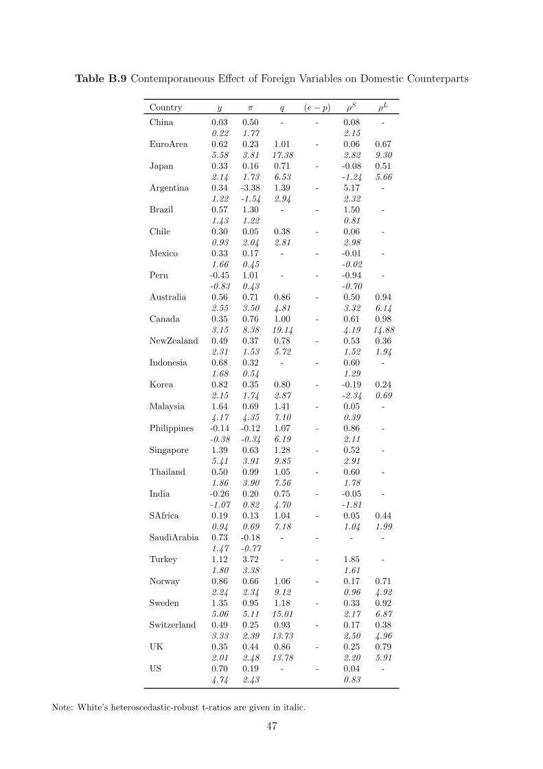
Table B.9 Contemporaneous Effect of Foreign Variables on Domestic Counterparts
Country y π q (e− p) ρS ρL
China 0.03 0.50 - - 0.08 -0.22 1.77 2.15
EuroArea 0.62 0.23 1.01 - 0.06 0.675.58 3.81 17.38 2.82 9.30
Japan 0.33 0.16 0.71 - -0.08 0.512.14 1.73 6.53 -1.24 5.66
Argentina 0.34 -3.38 1.39 - 5.17 -1.22 -1.54 2.94 2.32
Brazil 0.57 1.30 - - 1.50 -1.43 1.22 0.81
Chile 0.30 0.05 0.38 - 0.06 -0.93 2.04 2.81 2.98
Mexico 0.33 0.17 - - -0.01 -1.66 0.45 -0.02
Peru -0.45 1.01 - - -0.94 --0.83 0.43 -0.70
Australia 0.56 0.71 0.86 - 0.50 0.942.55 3.50 4.81 3.32 6.14
Canada 0.35 0.76 1.00 - 0.61 0.983.15 8.38 19.14 4.19 14.88
NewZealand 0.49 0.37 0.78 - 0.53 0.362.31 1.53 5.72 1.52 1.94
Indonesia 0.68 0.32 - - 0.60 -1.68 0.54 1.29
Korea 0.82 0.35 0.80 - -0.19 0.242.15 1.74 2.87 -2.34 0.69
Malaysia 1.64 0.69 1.41 - 0.05 -4.17 4.35 7.10 0.39
Philippines -0.14 -0.12 1.07 - 0.86 --0.38 -0.34 6.19 2.11
Singapore 1.39 0.63 1.28 - 0.52 -5.41 3.91 9.85 2.91
Thailand 0.50 0.99 1.05 - 0.60 -1.86 3.90 7.56 1.78
India -0.26 0.20 0.75 - -0.05 --1.07 0.82 4.70 -1.81
SAfrica 0.19 0.13 1.04 - 0.05 0.440.94 0.69 7.18 1.04 1.99
SaudiArabia 0.73 -0.18 - - - -1.47 -0.77
Turkey 1.12 3.72 - - 1.85 -1.80 3.38 1.61
Norway 0.86 0.66 1.06 - 0.17 0.712.24 2.34 9.12 0.96 4.92
Sweden 1.35 0.95 1.18 - 0.33 0.925.06 5.11 15.01 2.17 6.87
Switzerland 0.49 0.25 0.93 - 0.17 0.383.33 2.39 13.73 2.50 4.96
UK 0.35 0.44 0.86 - 0.25 0.792.01 2.48 13.78 2.20 5.91
US 0.70 0.19 - - 0.04 -4.74 2.43 0.83
Note: White’s heteroscedastic-robust t-ratios are given in italic.
47
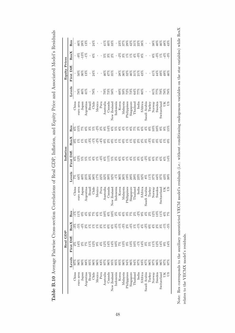
Table
B.1
0A
vera
gePai
rwis
eC
ross
-sec
tion
Cor
rela
tion
sof
Rea
lG
DP,In
flat
ion,an
dE
quity
Pri
cean
dA
ssoci
ated
Model
’sR
esid
ual
s
RealG
DP
Inflation
Equity
Pric
es
Levels
Fir
stD
iff.
ResX
Res
Levels
Fir
stD
iff.
ResX
Res
Levels
Fir
stD
iff.
ResX
Res
Chin
a97%
2%
-3%
-1%
Chin
a7%
6%
0%
6%
Chin
a-
--
-eu
roare
a96%
14%
-5%
11%
euro
are
a44%
12%
1%
15%
euro
are
a78%
50%
-9%
46%
Japan
90%
2%
-4%
0%
Japan
40%
5%
1%
7%
Japan
46%
36%
-13%
28%
Arg
enti
na
88%
7%
2%
4%
Arg
entina
25%
5%
3%
0%
Arg
entina
41%
13%
-1%
13%
Bra
zil
95%
11%
1%
9%
Bra
zil
20%
1%
-3%
3%
Bra
zil
--
--
Chile
96%
12%
1%
7%
Chile
38%
4%
-1%
5%
Chile
78%
24%
6%
24%
Mex
ico
96%
9%
1%
6%
Mex
ico
17%
1%
-2%
-2%
Mex
ico
--
--
Per
u83%
4%
2%
1%
Per
u22%
-4%
-4%
2%
Per
u-
--
-A
ust
ralia
97%
12%
1%
10%
Aust
ralia
32%
6%
0%
9%
Aust
ralia
79%
46%
5%
41%
Canada
96%
14%
0%
6%
Canada
39%
11%
2%
14%
Canada
73%
47%
3%
40%
New
Zea
land
95%
14%
6%
10%
New
Zea
land
32%
5%
0%
6%
New
Zea
land
58%
35%
2%
33%
Indones
ia95%
10%
-2%
2%
Indones
ia-1
%2%
1%
5%
Indones
ia-
--
-K
ore
a95%
7%
-1%
4%
Kore
a36%
6%
1%
8%
Kore
a69%
28%
-2%
23%
Mala
ysi
a96%
13%
-3%
6%
Mala
ysi
a26%
4%
0%
4%
Mala
ysi
a59%
36%
3%
37%
Philip
pin
es94%
3%
2%
3%
Philip
pin
es19%
1%
1%
1%
Philip
pin
es72%
32%
1%
29%
Sin
gapore
96%
13%
-4%
7%
Sin
gapore
29%
4%
1%
8%
Sin
gapore
73%
46%
1%
42%
Thailand
94%
10%
1%
2%
Thailand
29%
5%
0%
7%
Thailand
64%
31%
4%
31%
India
97%
-1%
-1%
-2%
India
23%
3%
2%
2%
India
77%
21%
-3%
22%
SA
fric
a93%
14%
4%
9%
SA
fric
a32%
6%
2%
6%
SA
fric
a80%
43%
8%
38%
SaudiA
rabia
87%
3%
-2%
4%
SaudiA
rabia
8%
-2%
3%
4%
SaudiA
rabia
--
--
Turk
ey96%
5%
0%
2%
Turk
ey11%
0%
-3%
0%
Turk
ey-
--
-N
orw
ay
97%
11%
4%
12%
Norw
ay
37%
6%
3%
10%
Norw
ay
81%
41%
8%
38%
Sw
eden
96%
12%
2%
13%
Sw
eden
44%
7%
3%
10%
Sw
eden
77%
44%
-3%
40%
Sw
itze
rland
96%
14%
3%
11%
Sw
itze
rland
37%
6%
4%
9%
Sw
itze
rland
79%
49%
1%
46%
UK
97%
9%
-1%
6%
UK
43%
6%
1%
9%
UK
78%
49%
-4%
48%
US
97%
14%
-5%
7%
US
39%
14%
0%
15%
US
78%
46%
-3%
43%
Not
e:R
esco
rres
pond
sto
the
auxi
liary
unre
stri
cted
VE
CM
mod
el’s
resi
dual
s(i
.e.:
wit
hout
cond
itio
ning
endo
geno
usva
riab
les
onth
est
arva
riab
les)
whi
leR
esX
rela
tes
toth
eV
EC
MX
mod
el’s
resi
dual
s.
48
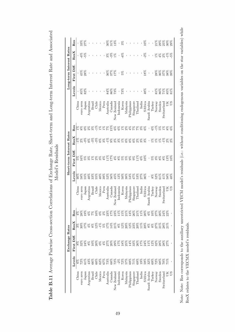
Table
B.1
1A
vera
gePai
rwis
eC
ross
-sec
tion
Cor
rela
tion
sof
Exch
ange
Rat
e,Shor
t-te
rman
dLon
g-te
rmIn
tere
stR
ate
and
Ass
oci
ated
Model
’sR
esid
ual
s
Exchange
Rate
sShort-
term
Inte
rest
Rate
sLong-t
erm
Inte
rest
Rate
s
Levels
Fir
stD
iff.
ResX
Res
Levels
Fir
stD
iff.
ResX
Res
Levels
Fir
stD
iff.
ResX
Res
Chin
a6%
8%
3%
4%
Chin
a46%
5%
-1%
1%
Chin
a-
--
-eu
roare
a72%
32%
30%
28%
euro
are
a58%
16%
2%
8%
euro
are
a85%
45%
-6%
33%
Japan
61%
24%
17%
19%
Japan
55%
5%
-3%
0%
Japan
82%
28%
-5%
27%
Arg
enti
na
43%
8%
4%
6%
Arg
entina
40%
3%
0%
2%
Arg
entina
--
--
Bra
zil
66%
10%
8%
7%
Bra
zil
33%
1%
-3%
3%
Bra
zil
--
--
Chile
60%
20%
12%
10%
Chile
55%
2%
-3%
-1%
Chile
--
--
Mex
ico
62%
0%
-1%
0%
Mex
ico
40%
3%
0%
1%
Mex
ico
--
--
Per
u67%
4%
5%
2%
Per
u39%
4%
3%
1%
Per
u-
--
-A
ust
ralia
73%
27%
17%
23%
Aust
ralia
52%
11%
-1%
7%
Aust
ralia
84%
36%
3%
30%
Canada
68%
20%
14%
17%
Canada
56%
17%
9%
15%
Canada
86%
37%
-3%
31%
New
Zea
land
72%
29%
21%
23%
New
Zea
land
45%
4%
2%
6%
New
Zea
land
73%
17%
1%
13%
Indones
ia-2
%17%
8%
11%
Indones
ia12%
8%
3%
6%
Indones
ia-
--
-K
ore
a72%
18%
12%
15%
Kore
a50%
5%
1%
1%
Kore
a73%
5%
-6%
3%
Mala
ysi
a57%
25%
20%
21%
Mala
ysi
a38%
5%
0%
2%
Mala
ysi
a-
--
-P
hilip
pin
es69%
14%
12%
13%
Philip
pin
es53%
9%
0%
4%
Philip
pin
es-
--
-Sin
gapore
71%
33%
23%
26%
Sin
gapore
47%
9%
0%
7%
Sin
gapore
--
--
Thailand
69%
26%
20%
21%
Thailand
53%
11%
2%
7%
Thailand
--
--
India
19%
17%
11%
11%
India
27%
6%
3%
3%
India
--
--
SA
fric
a59%
24%
20%
20%
SA
fric
a36%
10%
3%
6%
SA
fric
a48%
18%
-2%
10%
SaudiA
rabia
32%
11%
8%
6%
SaudiA
rabia
--
--
SaudiA
rabia
--
--
Turk
ey69%
12%
8%
10%
Turk
ey8%
5%
1%
6%
Turk
ey-
--
-N
orw
ay
72%
32%
27%
27%
Norw
ay
52%
3%
1%
-1%
Norw
ay
81%
28%
1%
21%
Sw
eden
68%
28%
21%
20%
Sw
eden
61%
8%
1%
5%
Sw
eden
86%
36%
4%
29%
Sw
itze
rland
70%
28%
28%
24%
Sw
itze
rland
41%
8%
-1%
1%
Sw
itze
rland
71%
37%
2%
25%
UK
71%
27%
21%
22%
UK
58%
13%
2%
8%
UK
85%
38%
-1%
30%
US
--
--
US
48%
10%
2%
6%
US
81%
39%
-5%
29%
Not
e:N
ote:
Res
corr
espo
nds
toth
eau
xilia
ryun
rest
rict
edV
EC
Mm
odel
’sre
sidu
als
(i.e
.:w
itho
utco
ndit
ioni
ngen
doge
nous
vari
able
son
the
star
vari
able
s)w
hile
Res
Xre
late
sto
the
VE
CM
Xm
odel
’sre
sidu
als.
49