On the use of linear graph theory in multibody system dynamics · On the Use of Linear Graph Theory in Multibody System Dynamics ... the fundamental cutset ... On the Use of Linear

Nonlinear Dynamics 9: 73-90, 1996. © 1996 Kluwer Academic Publishers. Printed in the Netherlands.

On the Use of Linear Graph Theory in Multibody System Dynamics

J. J. McPHEE Systems Design Engineering, University of Waterloo, Ontario, Canada N2L 3G1

(Received: 26 August 1994; accepted: 19 September 1994)

Abstract. Multibody dynamics involves the generation and solution of the equations of motion for a system of connected material bodies. The subject of this paper is the use of graph-theoretical methods to represent multibody system topologies and to formulate the desired set of motion equations; a discussion of the methods available for solving these differential-algebraic equations is beyond the scope of this work. After a brief introduction to the topic, a review of linear graphs and their associated topological arrays is presented, followed in turn by the use of these matrices in generating various graph-theoretic equations. The appearance of linear graph theory in a number of existing multibody formulations is then discussed, distinguishing between approaches that use absolute (Cartesian) coordinates and those that employ relative (joint) coordinates. These formulations are then contrasted with formal graph-theoretic approaches, in which both the kinematic and dynamic equations are automatically generated from a single linear graph representation of the system. The paper concludes with a summary of results and suggestions for further research on the graph-theoretical modelling of mechanical systems.

Key words: Multibody dynamics, linear graph theory, absolute and joint coordinates.

1. Introduct ion

A multibody system is hereby defined as afinite number of material bodies connected in an arbitrary fashion by mechanical joints that limit the relative motion between pairs of bodies. Practitioners of multibody dynamics study the generation and solution of the equations governing the motion of such systems. Several different approaches for systematically formulating these equations of motion have been developed, and encoded in numerical or symbolic computer programs. Such programs relieve an analyst of the error-prone labour involved in deriving the governing differential-algebraic equations by hand. For the program to be applicable to a wide range of mechanical systems, the topology of which is specified by the user at execution time and is not known apriori, the underlying formulation must somehow represent the connectivity of the system and use this topological information during the derivation of the equations of motion.

Linear graph theory is that branch of mathematics that studies the description and manip- ulation of system topologies. Interestingly, the extent to which this theory has been incorporated into current multibody dynamic formulations ranges from a bare minimum, typically in approaches that use absolute coordinates to describe the motion of each body, to a maximum in formal graph-theoretic procedures. It is the goal of this paper to examine this apparent conundrum in some detail, by explicit referring to a number of existing formulations.

The paper begins with a brief review of finite directed linear graphs and associated mathematical theorems, followed by a discussion of the minimal use of such graphs in absolute coordinate formulations. This in turn is followed by an examination of how linear graphs are used to represent system topologies in formulations that employ relative joint variables as generalized coordinates. Finally, a number of approaches that rely entirely on graph-

74 J. J. McPhee

L 1

V7 ( t ) ~ .,, C6

T ,A/V"

R 3

R 4

R 5 L 2

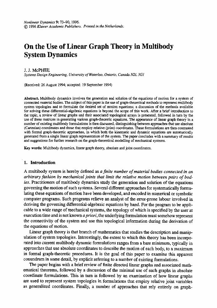
Fig. 1. Electrical network example.

theoretic techniques to automatically formulate the equations of motion are described. The paper concludes with a summary of results and suggestions for future exploitation of linear graph-theoretic methods in multibody dynamics.

2. Review of Graph-Theoretical Methods

The study of linear graph theory, one branch of the wider field of combinatorial mathematics, originated with Euler's famous solution [ 1 ] to the problem of the Ktnigsberg bridges in 1736. A complete review of the contributions to linear graph theory since then is beyond the scope of this article. Instead, attention will be directed on those graph theorems that have application to the dynamic analysis of multibody systems. In consideration of the previous definition of a multibody system as a finite number of connected bodies, a discussion of infinite or unconnected graphs is excluded from this review. Furthermore, attention will be restricted to the study of directed graphs, since their undirected counterparts find less application in multibody dynamics. In summary then, the following review is limited to connected finite directed linear graphs and their associated mathematical theorems. For a more complete discussion of linear graph theory and its application to physical systems analysis, the reader is directed to [2-5].

2.1. REPRESENTATION OF TOPOLOGY

A linear graph is a collection of edges, no two of which have a point in common that is not a vertex. In turn, an edge is defined as a line segment together with its distinct endpoints, and a vertex (or node) is an endpoint of an edge. The topology of a linear graph is completely defined when one specifies which edges are incident upon (connected to) each and every vertex of the graph.

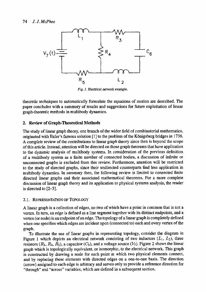
To illustrate the use of linear graphs in representing topology, consider the diagram in Figure 1 which depicts an electrical network consisting of two inductors (L1, L2), three resistors (R3, R4, Rs), a capacitor (C6), and a voltage source (~) . Figure 2 shows the linear graph which is topologically equivalent, or isomorphic, to the electrical network. This graph is constructed by drawing a node for each point at which two physical elements connect, and by replacing these elements with directed edges on a one-to-one basis. The direction (arrow) assigned to each edge is arbitrary and serves only to provide a reference direction for "through" and "across" variables, which are defined in a subsequent section.

On the Use of Linear Graph Theory in Multibody System Dynamics 75

@ ® @

L 1 R3

V 7 R 4 C 6

(5 R 5 ® Fig. 2. Linear graph isomorphic to electrical network.

From the linear graph, one can construct the incidence matr ix [IN] which contains a complete topological description of the original physical system. This is a v x e matrix, where v is the number of vertices in the graph, and e is the number of edges. The (i,j) entry in [IN] is equal to ( - 1, + 1,0) if edge j is (negatively, positively, not) incident upon node i. The directed edge j is positively incident upon node i if it points towards the node, and negatively incident if it is directed away from the node. As an example, the incidence matrix for the linear graph in Figure 2 takes the form:

L1 L2 R3 R4 R5 C6 V7

a

b C

[ m ] = d e

y

- 1 0 0 1 0 1 0 0 - 1 0 1 0 0 - 1 0 0 0 0

0 0 0 1 1 0 0 0 0 0 - 1 0 0 0 1 0

- 1 1 0 0 0 - 1 0 - 1

(1)

in which the vertices associated with rows and the edges associated with columns have been explicitly labelled. One can see from this example that the rows of [IN] are not linearly independent, since their sum is a row containing all zeroes. The (v - 1 ) × e reduced incidence matr ix [A] is obtained by deleting any one row of [IN]; the remaining rows of [A] are linearly independent, and the vertex corresponding to the deleted row is referred to as the datum node.

An important concept in linear graph theory is that of a circuit, which is a subset of a graph (or subgraph) such that, on every vertex, there are incident exactly two edges. In other words, a circuit is a closed loop of edges. With this concept, one can define a spanning tree, which is a subgraph containing all the vertices of the original graphs, but no circuits. The (v - 1 ) edges in a tree of the graph are called branches, whereas the remaining edges in the complement of the tree, or cotree, are known as chords. One possible spanning tree for the graph in Figure 2 has been drawn with thick lines and consists of edges Li , L2, R3, R4, and Rs. The remaining edges C6 and V7 comprise the chords of the cotree. Having defined the concept of a tree, two new topological matrices can now be introduced - the fundamental cutset matrix and the fundamental circuit matrix.

76 J. J. McPhee

A cutset is a subgraph of a connected linear graph such that, when deleted, the graph is left in two distinct parts. A fundamental cutset, or f-cutset, is a cutset consisting of one branch from the tree and a minimal number of chords such that no subgraph of the cutset is itself a cutset. As an example, the f-cutset corresponding to branch L1 in Figure 2 consists of LI and V7 (note that node @ is not deleted along with the cutset edges and constitutes one of the two remaining parts of the graph). There will be (v - 1 ) f-cutsets for a given linear graph and tree, from which one can construct the fundamenta l cutset matr ix [CU]. The (i, j) entry of [CU] is zero if edge j is not in the f-cutset corresponding to branch i, and ( - 1, + 1 ) if edge j is in the f-cutset and has the (opposite, same) orientation as branch i. With this definition, the (v - 1) × e matrix [CU] takes the general partitioned form:

[CU] = [[lt] I [A~]], (2)

in which [lt] is a square unit matrix corresponding to the tree branches in the first (v - 1) columns, and [Ac] is the remaining (v - 1) x (e - v + 1) submatrix. For the linear graph in

~ n d a m e n t a l c u t s e t m a ~ x ~ e s t h e s p e c i f i c f o r m : [00000 0 1 0 0 0 1

[CU]= 0 0 1 0 0 1 . (3) 0 0 0 1 0 - 1 0 0 0 0 1 0

Figure 2, the

An important result from linear graph theory is that the fundamental cutset matrix [CU] is row- equivalent to the reduced incidence matrix [A]. In other words, [CU] need not be constructed using its definition - it can be obtained through simple row operations on [A]. Verification of this theorem for the linear graph in Figure 2 is left to the reader.

A fundamental circuit, or f-circuit, is a circuit in which one edge is a chord from the cotree of the graph, and all the remaining edges are branches. To illustrate, the f-circuit corresponding to chord C6 in Figure 2 also contains branches L2, R3, and R4. There will be (e - v + 1) f-circuits for a given graph and tree, from which the fundamenta l circuit matr ix [CI] can be constructed. The (i, j ) entry of [CI] is zero if edge j is not in the f-circuit corresponding to chord i, and ( - 1, + 1 ) if edge j is in the f-circuit and has the (opposite, same) direction as chord j as one travels around the circuit. With this definition, the (e - v + 1 ) × e matrix [CI] can be written in the general form:

[CI] = [[Bt] I [lc]], (4)

where [lc] is a square unit matrix corresponding to the cotree chords, and [Bt] is the remaining (e - v + 1 ) x (v - 1 ) submatrix. The specific form of [CI] for the example in Figure 2 is:

[ C I ] = [ 0 - 1 - 1 1 0 1 0 ] 1 0 0 - 1 - 1 0 1 " (5)

Another important linear graph theorem [6] states that the rows of the circuit and cutset matrices for a given graph and tree are orthogonal, or mathematically,

[C1][CU] T = [0] (6)

in which the superscript T represents the transpose operation, and [0] is a (e - v + 1 ) x (v - 1) matrix containing all zeroes. Substituting equations (2) and (4) into equation (6) and re- arranging, one can show that:

[Bt] = -[Ac] T, (7)


which can be verified for the linear graph in Figure 2 by examining the specific form of equations (3) and (5).

In summary, the incidence matrix [IN] contains a complete topological description of a given linear graph. The nonsingular reduced incidence matrix [A] is obtained by deleting a row of [IN] corresponding to the datum node. By selecting a spanning tree and numbering the first (v - 1 ) columns of [A] to correspond to the branches, the fundamental cutset matrix [CU] can be obtained through simple row operations. This topological matrix explicitly shows (v - 1 ) independent ways in which the given linear graph can be cut into two distinct parts - a result that is used later in this paper to generate the force equilibrium equations for mass elements in a multibody system without actually constructing the corresponding free-body diagrams. The fundamental circuit matrix [CI] can, in turn, be obtained directly from [CU] using equation (7) to construct the [Bt] submatrix. Upon completion, [CI] can be used to identify an independent set of (e - v + 1) circuits in the given graph, an application of particular relevance to the kinematic analysis of multibody systems with closed loops.

2.2. GRAPH-THEORETICAL EQUATIONS

The circuit, cutset, and incidence matrices have more than topological significance - they can also be used to generate the governing equations for the physical system to which the linear graph is isomorphic. This fact was recognized almost four decades ago by Trent [5], who introduced the concept of through and across variables in order to set up these equations.

A through variable is a physical variable, associated with an edge of a graph, that would be measured by an instrumental placed in series with the corresponding element in the original network. In the electrical network example in Figure 1, an appropriate through variable would be the current through an element. For a multibody system, the relevant through variables are forces or torques. Regardless of the type of physical system, the above definition of a through variable guarantees that the "Vertex Postulate", which states that the sum of through variables at any node of a system graph must equal zero when due account is taken of the orientation of edges incident upon that node, is satisfied for the linear graph. Essentially, the Vertex Postulate represents a generalization of Kirchhoff's Current Law, from electrical network theory, that is applicable to all physical systems. It can be expressed mathematically for all v nodes in a graph by premultiplying the column matrix of through variables {T} by the incidence matrix:

= {0), (8)

where {0} is a v x 1 column matrix of zeroes. To obtain a linearly independent set of equations in the through variables, [IN] in equa-

tion (8) can be replaced by either the reduced incidence matrix [A] or the cutset matrix [CU]. In the latter case, and using equation (2), the resulting equations can be solved explicitly for the (v - 1) through variables {Tt} associated with the branches:

{Tt} = --[A~]{T~} (9)

in which {re} are the cotree through variables. If these latter variables are known, then {rt} can be calculated directly from equation (9). It is for this reason that the cotree and tree

78 J. J. McPhee

through variables are referred to as "primary" and "secondary" variables, respectively. Using equation (3) for the electrical network example, equation (9) takes the specific form:

r3 = r6 , (10)

7" 4 --7"6 -÷- T7

7-5 T7

which is equivalent to the set of equations obtained by successive applications of Kirchhoff's Current Law to the network.

An across variable associated with an edge is a physical variable that would be measured by an instrument placed in parallel with the corresponding element in the physical network. In electrical systems, voltage is the most common example of such variables, whereas in multibody systems, relative displacements, velocities, and accelerations are all appropriate across variables. In general, the derivatives and integrals of across variables are themselves across variables, as are vectors whose scalar components correspond to across variables. A rigorous definition of across variables is that they satisfy the "Circuit Postulate", namely that the sum of across variables around any circuit of a graph must equal zero when due account is taken of the direction of edges in the circuit.

To obtain a linearly independent set of equations that are mathematically equivalent to the Circuit Postulate, one need only premultiply a column matrix of across variables {a} by the circuit matrix, and set the result to {0}:

[CI]{a} = {0}. (11)

Equation (4) can be used to express the (e - v + 1 ) across variables associated with the chords {ac} as explicit functions of the tree across variables {at}:

{c~c} = -[St]{at}, (12)

which is why {at} is added to the list of primary variables, and {ac} is a subset of the secondary variables. Using equation (5) for the electrical network example, equation (12) takes the form

0~7 --0~1 + 0:4 + 0~5 '

which is equivalent to the independent set of equations obtained by applying Kirchhoff's Voltage Law to the inner two loops of the network.

With e primary variables and another e secondary variables, the total number of unknowns is 2e. Available for the solution of these unknown quantities are the (v - 1 )cutset equations (9) and the (e - v + 1) circuit equations (12) - a total of e linearly independent equations. The remaining e equations required to effect a solution are obtained from the constitutive, or terminal, equations for each of the e elements in the system. The terminal equation for each element expresses the functional relationship between the through and across variables and the independent variable, time. As an example, the terminal equation for the ideal inductor L1 shown in Figure 1 would be:

L dT-1 (14)


%

P2

T(

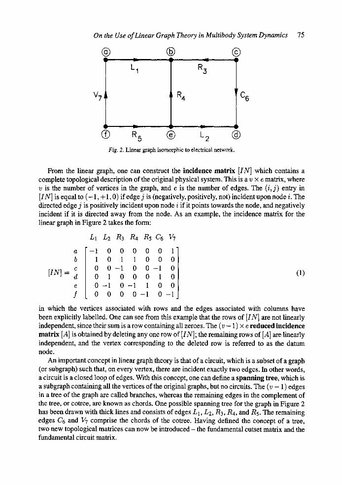
Ply/ ' F~/P4 Fig. 3. Torque-driven planar four-bar mechanism.

79

where cq corresponds to the voltage across L1, and rl represents the current passing through the inductor. For a three-dimensional multibody system, the through and across variables are spatial vectors and the corresponding terminal equations are vectorial relationships. Regardless of the type of system under study however, the circuit, cutset, and terminal equations comprise a necessary and sufficient set for the solution of all unknown variables as functions of time [6]. The advantage of using these formal graph-theoretic techniques over traditional methods of formulating the governing equations is twofold:

1. the topological equations are clearly separated from the constitutive equations for the elements comprising the physical system under study, and

2. there is a number of standard graph-theoretic formulations available in the literature [2-5] for systematically establishing the governing equations - the particular choice of formulation method is made based upon the desired final form of these equations.

Finally, one may add that the systematic nature of formal graph-theoretic approaches make them quite attractive if a computer implementation is desired.

Before ending this review of linear graph theory, an auxiliary set of nodal variables are introduced. Essentially, a nodal variable corresponds to a physical variable that would be measured by an instrument placed between (across) the relevant node and a reference datum node. For an electrical network, the voltage difference between a node and the ground would be classified as a nodal variable. In a multibody system, the absolute displacement, velocity, or acceleration of a point relative to an inertial reference frame all represent nodal variables. The reduced incidence matrix [A] provides a convenient means for transforming between the nodal {r;} and across {o~} variables of a system graph:

{a} --[A]T{~}. (15)

The nodal transformation equation (15) increases the total number of available equations by ( v - 1), which corresponds to the additional ( v - 1 ) unknowns, the auxiliary nodal variables.

3. Absolute (Cartesian) Coordinate Formulations

Attention is now switched to the other main topic of this paper, the dynamics of multibody systems. An example of such a system is the planar four-bar mechanism shown in Figure 3, which consists of three rigid links connected by ideal revolute joints to form a closed loop

80 J. J. McPhee

Y

""2y

Fig. 4. Free-body diagram of link 2.

=- R3x

with the ground (the fourth "bar"). Assuming that a time-varying torque T(t) is applied to link 1, the goal of a dynamic analysis would be to determine the configuration of the system at each instant during a finite interval of time. To represent the configuration, a set of coordinates that uniquely describe the position of each body in the system must be defined. The dynamic analysis is accomplished by generating the differential-algebraic equations (DAEs) of motion and solving them for the time-varying coordinates. This procedure has been successfully automated in a number of existing multibody programs using a variety of different formulation approaches.

Several of these approaches make use of absolute coordinates, which describe the position and orientation of each body in the system relative to an inertial frame of reference. For body 2 of the planar four-bar mechanism, shown in Figure 4, the absolute coordinates are defined as the Cartesian coordinates (x2, Y2) of the mass center C2 in the inertial X Y reference frame, as well as the angle 02 between the link and the positive X axis. With three absolute variables per body, the total number of system coordinates {p} is nine. Obviously, these nine coordinates are not independent since the four-bar mechanism has only one degree of freedom. The motion of individual bodies is constrained by the presence of kinematic joints between adjacent links; relationships between the absolute coordinates are obtained from a consideration of these holonomic constraint elements. Specifically, each pin joint requires that connected end points of adjacent bodies remain coincident during any motion of the system. Mathematically, for the kinematic pair consisting of bodies i - 1 and i connected by pin joint/~:

li 1 ¢'2i-1 = xi-1 + - ~ - cosOi_l - xi + cosOi = 0 (16)

li-1 li (~2i = Yi-1 -F T sin~9i_l - Yi + "~ sin0i = 0, (17)

noting that li is the length of uniform link i, the terms lo, 00, 14 and ~4 are constants defining the positions of pins/°1 and P4 in the inertial reference frame, and xo, Yo, x4, and y4 are all identically zero.

Assembling equations (16) and (17) for the four pin joints results in a set of eight nonlinear algebraic equations:

{(I)(p)} = {0}, (lS)

which, by themselves, are not sufficient to solve for the nine absolute coordinates. To obtain a second set of equations for the system, one can write the equations of motion for each body


in the system, by applying the Newton-Euler equations to a free-body diagram of each link. Note that the reaction forces {R} in the pin joints enter explicitly into these expressions. Assembling the nine differential equations for all three bodies into a matrix form gives

[M,~]{~} + [J]T {R} = {Qa}, (19)

in which [Ma] is the generalized mass matrix, {Qa} contains the applied forces and torques, and [J] is the Jacobian matrix of the constraint equations (18). In explicit form, the entries of [J] are given by

0¢9i Jij = Opj (20)

Together, equations (18) and (19) constitute a set of 17 differential-algebraic equations that can be solved for the nine absolute coordinates {p} and eight reaction forces {R} as functions of the independent variable, time.

The approach described above has been extended and applied to the analysis of three- dimensional systems of rigid and flexible bodies connected by a wide variety of general holonomic and nonholonomic joints [7-13]. Due to its simplicity, this formulation can be readily implemented in a computer program that automatically generates the governing DAEs for a given mechanical system. A library of constraint equations for a variety of kinematic joints can be created in advance and used to generate the relationships between the absolute coordinates of two bodies connected by a particular type of joint. A second library containing the corresponding Jacobian matrix for each joint can also be created, and used to generate the system Jacobian matrix [J] by means of an assembly process similar to that employed by the finite element method. The generalized mass matrix [Ma] and forcing vector {Qa} can be constructed directly from the input data provided by a user. Thus, all terms in the governing equations (18) and (19) can be obtained without using methods from linear graph theory. As Haug [9] has observed, the use of absolute coordinates in the underlying formulation results in a "bypassing [of] topological analysis".

Oflandea et al. [10] have used an even larger set of absolute coordinates than that described above in order to maximize the sparsity of the resulting DAEs, which are subsequently solved using sparse matrix methods and an implicit numerical integration routine. It is worth noting that these authors make explicit reference to the similarity between their derived equations and those arising in linear graph theory; specifically, they observe that equation (19) from their paper represents an assembly of the circuit, cutset, and terminal equations that would be obtained from a network model of their multibody system. In spite of this comparison, the authors assemble their equations without exploiting the systematic nature of a graph- theoretical approach. G6radin [11] uses absolute coordinates in a finite element formulation of the equations of motion for flexible multibody systems. Once again, the use of such coordinates eliminates the need for linear graph theory since, as the author points out, "the topology of the articulated system is automatically embedded into its finite element description".

4. Relative (Joint) Coordinate Formulations

A second means of representing the time-varying configuration of a multibody system is through the use of relative coordinates. These coordinates describe the relative position and orientation of two adjacent bodies in terms of variables associated with the kinematic joint connecting the two bodies. A joint that allows j degrees of freedom (where j < 6) contributes

82 J. J. McPhee

j variables to the set of system relative coordinates {q}. As an example, the relative rotation between any two links in Figure 3 can be described by a single angle ¢ corresponding to the revolute joint connecting the two links. The complete set of three relative coordinates for this four-bar mechanism can be defined in terms of the previous absolute coordinates:

q~l = 01

t~2 ----- 02 - - 0 1

¢3 = 03 - 02 (21)

corresponding to pin joints P1, P2, and P3. Note that it is not necessary to define the position of link 4 (the ground) relative to link 3.

If the multibody system has no closed loops, i.e. it has a "tree" topology, the set of relative coordinates is equal in number to the degrees of freedom of the system. As an example, if pin P4 were removed from the four-bar mechanism, the resulting open-loop system would have three degrees of freedom. Using relative coordinates {q}, the equations of motion for such a system can be written in the form

[Mr]{~} = {Qr(q,(l , t)}, (22)

noting that reaction forces and torques in the joints have been eliminated from these equations using either an analytical approach (e.g. d'Alembert's Principle or Lagrange's equations) or a systematic substitution process [14] in conjunction with the Newton-Euler equations. Equation (22) constitutes a set of ordinary differential equations that can be numerically integrated to obtain the relative coordinates as functions of time.

These same equations can be used to derive the DAEs governing the motion of a multibody system with closed loops. In this case, the relative coordinates are no longer independent and are related by the set of nonlinear algebraic constraint equations:

{ffl(q)) = (0} (23)

corresponding to the equations guaranteeing closure of an independent set of loops. For the four-bar mechanism, these loop closure equations can be obtained by summing the eight joint constraint equations (16) and (17), resulting in

I0 cos 00 + I1 cos 01 + 12 cos 02 + 13 cos 03 - 14 c o s 04 = 0 (24)

10 sin 00 + Ii sin 01 + 12 sin 02 + 13 sin 03 -- 14 sin 04 = 0. (25)

Defining two new constants Cz and Cy that represent the distance between pins P1 and P4 in the X and Y directions, respectively,

C~c = 14 c o s 04 - 10 c o s 00 (26)

C v = t4 sin 04 - lo sin 00 (27)

and using equations (21) to replace the absolute coordinates with their relative counterparts, the constraint equations (24) and (25) can be written in the desired form:

ffJl = /1 cos ¢1 + 12 cos(q~1 + ~2) + 13 cos(~bl + ¢2 + q~3) - Cx = 0 (28)

~2 = 11 sin ~bl + t2 sin(q~l + ~b2) + t3 sin(~bl -t- q~2 + ~3) - Cy = 0. (29)


The final set of DAEs is obtained by removing from the system model one kinematic joint for each independent closed loop. The motion of the resulting open-loop system is governed by equation (22). By adding to this equation terms corresponding to the reaction forces and torques in the joints that were removed, the differential equations for the original system with closed loops are obtained:

[M~]{~} + [K]T{A} = {Q~}, (30)

where {A) is a set of Lagrange multipliers, and [K] is the Jacobian matrix of the loop closure constraint equations:

Kij = .Oqj • (31)

Equations (23) and (30) constitute the final set of DAEs for the multibody system, expressed in terms of relative coordinates. One can see that they are similar in form to the corresponding equations (18) and (19) in absolute coordinates, but are generally fewer in number. The generalized mass matrix [M,.] is smaller and less sparse than its absolute counterpart [Ma], and the generalized forcing vector {Qr} is a complex function of the relative coordinates, their derivatives, and time. Even though the loop closure equations (23) have a higher order of nonlinearity than the constraint equations (18), the smaller set of DAEs for relative coordinates can be solved more efficiently than its counterpart in absolute coordinates. However, as Nikravesh [8] has pointed out, this computational advantage is offset by the additional labour required to generate these equations.

One source of this additional labour is the requirement for topological processing when relative coordinates are employed. The reason for this is simple: regardless of the type of approach one uses to derive the differential equations (30), one needs expressions for the velocity (e.g. to formulate the kinetic energy for use with Lagrange's equations) or the acceleration (e.g. using the Newton-Euler equations) of each body relative to an inertial frame of reference. For a particular body mi, one can obtain these expressions from the relative coordinates and their time derivatives only if one knows the identity and ordering of the intermediate bodies connecting mi to the inertial reference frame. In brief, a mathematical description of the system topology is required; such a description is conveniently provided by linear graph theory.

Sheth and Uicker [15] recognized this fact over two decades ago, when they used Hamil- ton's Principle and relative coordinates to formulate the differential equations for a multibody system consisting entirely of closed kinematic loops. To obtain the supplementary set of loop closure constraint equations, the authors construct a simple linear graph representation of the multibody system, in which nodes represent links and edges represent kinematic joints. With this linear graph, the authors are able to derive an independent set of loop closure equations that are equivalent to the fundamental circuit equations, with the relative coordinates play- ing the role of across variables. Furthermore, a graph-theoretical algorithm is employed to minimize the number of joints appearing in the final set of independent loops. It is possible to identify further equivalences between the equations derived by Sheth and Uicker and the graph-theoretical circuit and cutset equations; the interested reader is referred to the thesis by Li [16].

In the first monograph on multibody systems, Wittenburg [14] makes direct use of linear graph theory to represent the topology of a system of rigid bodies containing both open and

84 J. J. McPhee

m 2

m 1 m 3

m 0

Fig. 5. Wittenburg's linear graph of four-bar mechanism.

closed kinematic loops. Similar to the model employed by Sheth and Uicker, rigid bodies are represented as nodes of the graph and hinges between bodies appear as edges. Wittenburg's graph model is more encompassing however, since his "hinge" has been generalized to include springs, dampers, and other connections having six degrees of freedom. In addition, Wittenburg makes explicit use of a "spanning tree" that is consistent with conventional graph-theoretic methods. For the four-bar mechanism, the linear graph thus defined takes the form shown in Figure 5. The four nodes have been labelled as mi, where mi represents link i, and the hinges labelled Pj correspond to the four pin joints. The edges comprising an arbitrarily-selected tree are drawn as solid lines, while the one cotree edge is dashed.

To represent the system connectivity, Wittenburg defines an incidence matrix [W] that takes the general form

EI 011E ] [w] = [s] [s*] (32)

or specifically, for the linear graph of the four-bar mechanism

1 0 0[ 1

-1 1 01 0 [W] = 0 -1 1 0 (33)

0 0 -1 -1

Upon examination, one can see that the matrix [W] is exactly the negative of the incidence matrix [IN] defined in Section 2 of this paper. The first row of [W] corresponds to the datum node, and the (*) superscript is used to identify hinges in the cotree of the graph. Therefore, the n × n submatrix [S], where n is one less than the number of nodes (bodies) in the system, represents the tree portion of the reduced incidence matrix [A]. The inverse of this matrix was first introduced by Branin [17] and called the "node-to-datum-path matrix", since it can be constructed by examining which edges lie in the path between a given node and the datum node.


Unaware of Branin's previous work, Roberson and Wittenburg [18] re-invented this matrix, called it simply the "path matrix" [T], and verified the relationships

[T]T[So] T = - { 1 } (34)

IT]IS] = [Sl[T] = [1], (35)

where {1} is a column matrix of n elements, each equal to 1, and [1] is the n x n identity matrix. Wittenburg [14] makes extensive use of the [S] and [T] matrices to derive the differential equations (30) for a multibody system. Unfortunately, the generation of the constraint equations (23) is only presented by way of three example analyses. This drawback was subsequently addressed in [19], in which Wittenburg presents a systematic procedure for formulating the loop closure equations, once again making use of the topological matrices [S] and IT].

It is interesting to note that formal graph-theoretic methods can be used to derive many of the equations appearing in Wittenburg's formulation. To do so, one must identify a set of through and across variables [5] that respectively satisfy the vertex and circuit postulates for Wittenburg's linear graph. The relative rotational velocities {f2} form a natural set of across variables for this graph, and must therefore satisfy the fundamental circuit equation (12):

= (36)

where {Qc} and {Qt} correspond to hinges in the cotree and tree, respectively. Recalling equation (7) and using the interesting fact [17, 19] that the path, reduced incidence, and cutset matrices are related by

[T][S*] = [At], (37)

one can verify that equation (36) is identical to Wittenburg's equations (5.211), which is used to find an expression for the virtual work done in cut (cotree) hinges.

An appropriate nodal variable for Wittenburg's graph is the difference between the absolute angular velocity of each body and that of the base body (node):

~/i = _wi - w__0. (38)

A subset of the nodal transformation equation (15) can be used to relate this set of nodal variables {~/} to the tree across variables {ftt ), if one recognizes that -[S] corresponds to the tree portion of the reduced incidence matrix [A]:

{~-~t } = - - [ s ]T({~} -- W---0{ 1 }). (39)

Premultiplying equation (39) by -[T] T, one obtains Wittenburg's equation (5.122):

{w} = -[T] T{f2t} + w0{1 }, (40)

which is subsequently used to obtain the differential equations (22) for the open-loop (tree) portion of the multibody system. For a further discussion of the relationships between Wit- tenburg's formulation and formal graph-theoretic methods, the reader is directed to the forth- coming paper [20].

If one is only interested in using the topological description to generate kinematic relationships, then alternatives to a linear graph representation are available in the literature. As

86 J. J. McPhee

an example, the tree topology of an open-loop multibody system is represented by Huston and Passerello [21] using a "body connection array", which is subsequently employed by Amirouche [22] to generate the loop closure equations for a general system of rigid and flexible bodies. Nikravesh and Gim [23] transform the absolute coordinate DAEs (18) and (19) to the set of equations (23) and (30) in relative coordinates using a topology-dependent velocity transformation matrix; Kim and Vanderploeg [24] have presented a systematic procedure for constructing this matrix using a modified version of the path matrix [T], in which all - 1 's are replaced by +1 's. Pereira and Proen~a [25] have applied a similar transformation to the DAEs for a multibody system containing rigid and flexible members. Hiller et al. [26] have presented an alternative means of transforming the equations from absolute to relative to (in some instances) minimal coordinates, using the concept of a "kinematical transformer" to represent a closed loop; the topology of the complete system is contained in a block diagram of these kinematical transformer elements.

Using a linear graph representation similar to that employed by Wittenburg, Hwang and Hang [27] have developed a recursive formulation for a system of rigid bodies with closed loops, and implemented this formulation on a computer with parallel processing capabilities. In a subsequent formulation for flexible multibody systems, Lai et al. [28] achieved a greater degree of parallelism by defining an "extended graph" in which nodes represent reference frames attached to bodies and edges represent the transformations between these frames. It is interesting to note that this graph representation is very similar to the "vector-network model" first introduced by Andrews and Kesavan [29], which is discussed further in the next section.

5. Graph-Theoretic Multibody Formulations

In the previous section, it was shown how a number of current multibody dynamics formulations use linear graph theory to represent the system topology and to generate various kinematic relationships. The difference between such approaches and a formal graph-theoretic procedure has been summarized by Li [16]:

To appreciate the difference between an ad hoc application of graph theory to dynamics and a graph-theoretic approach, one must understand that a terminal graph (edge) is part of a mathematical model of a physical component. If the individual system components are modelled properly, the resulting system graph will automatically satisfy the cutset and circuit postulates.

As discussed in Section 2, if each edge is associated with a physical component and a consistent set of through and across variables is chosen, then a graph-theoretic formulation will automatically provide a necessary and sufficient set of DAEs. In the formulation discussed in the previous section, the edges did not correspond to physical components but simply represented the connectivity of the system. It is impossible to obtain the dynamic equations of motion directly from such a linear graph.

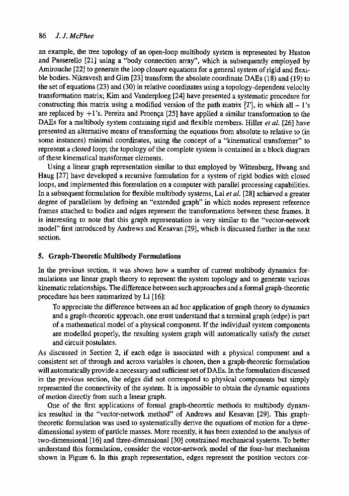
One of the first applications of formal graph-theoretic methods to multibody dynamics resulted in the "vector-network method" of Andrews and Kesavan [29]. This graph- theoretic formulation was used to systematically derive the equations of motion for a three- dimensional system of particle masses. More recently, it has been extended to the analysis of two-dimensional [ 16] and three-dimensional [30] constrained mechanical systems. To better understand this formulation, consider the vector-network model of the four-bar mechanism shown in Figure 6. In this graph representation, edges represent the position vectors cor-


(~)~'~h'l 5

®),-® \=,o

h13 h16

Fig. 6. Vector-network graph of four-bar mechanism.

87

responding to physical components while nodes represent connection points between these components. In addition to representing the three rigid bodies therefore, the edges ml, m2, and m3 locate the mass centers of these links relative to a datum node @ fixed in inertial space. Similarly, edges r4 and r5 represent the points where pins/91 and P4 attach to the ground. The "rigid-arm" elements s6 to Sn correspond to body-fixed position vectors from the mass centers to the points on each body where the revolute joints are connected. The driving torque is represented by the edge T12, while the remaining edges hi3 to hi6 correspond to pin joints Pl to P4, respectively.

The vector-network graph is significantly more complex than its counterpart in Figure 5 because it contains dynamic, as well as kinematic, information. The existence of torque and mass elements in the vector-network model is evidence of this. Of course, the vector-network graph also contains the topological information provided by Wittenburg's graph, which can be recovered from Figure 6 by deleting the dynamic mass and torque elements, and contracting each combination of kinematic joint and connected rigid-arm elements into a single edge.

To generate the system equations using a graph-theoretic approach, a tree is selected that contains elements 1 to 11, with the torque and kinematic joint elements placed in the cotree. A suitable across variable is the position vector r__ i corresponding to element i in the graph, while the force __F i in this element is identified as an appropriate through variable. For each pin joint element hi, one can write the terminal equation:

_r i = O, (41)

recognizing the fact that the two points (nodes) connected by a revolute joint remain coincident for any possible motion of the system. With this terminal equation, the kinematic constraint equations can be systematically generated using the fundamental circuit equations (12) for the cotree pin joints. As an example, the circuit equation corresponding to kinematic joint hi4 (/:'2) is

/ '14 ~- 7"8 -~ I'2 - - 7"1 - - r--7 = 0 . ( 4 2 )

The eight constraint equations (16) and (17) are obtained by resolving the vectorial circuit equations for the four pin joints into components parallel to the inertial X and Y axes. In a

88 J. J. McPhee

similar systematic fashion, and recognizing the fact that the terminal equations for the mass elements corresponds to the vectorial Newton-Euler equations, the cutset equations for these tree elements result in nine scalar differential equations in which the reaction forces in the pin joints appear explicitly. One can see that, as a consequence of using absolute coordinates to represent the position and orientation of each mass element, the final set of DAEs generated by the vector-network method corresponds exactly to equations (18) and (19).

Using an analytical substitution procedure, Li [16] has reduced this set of DAEs to the smaller set corresponding to equations (23) and (30). More recently, McPhee [31 ] has directly derived these latter equations in relative coordinates by simply using a different tree selection scheme in a formal application of the vector-network method. As discussed in Section 2 and demonstrated above, such an approach provides a systematic formulation procedure in which the topological equations are clearly distinguished from the constitutive equations. This has the important implication that new types of mechanical elements, modelled by suitable terminal equations, can be incorporated into the multibody system model without altering the underlying formulation procedure. With this in mind, efforts are currently underway to incorporate nonholonomic joints, flexible bodies, and variable-mass elements into existing vector-network formulations. One further advantage of a graph-theoretic approach is that it can provide a single unified formulation for systems containing elements from different physical regimes, e.g. hydraulic, pneumatic, or electronic elements. This leads the author to be optimistic about the future application of graph-theoretic methods to the growing field of mechatronics.

6. Summary and Conclusions

To develop a dynamic formulation that is applicable to general multibody systems with open and closed loops, some means of representing the topology of the system is required. If one uses absolute coordinates to describe the location of bodies in the system, the topological description is automatically embedded in the relatively large set of DAEs. If one uses a set of relative (joint) coordinates however, some form of topological processing is required in order to account for the connectivity of the bodies. To represent the system topology and to generate some of the required kinematic relationships, several researchers have made use of linear graphs and their associated topological matrices. It has been shown that many of these kinematic relationships are equivalent to the equations obtained from a formal graph- theoretic approach. The advantages of using such an approach have been discussed, and the systematic generation of the governing DAEs using the vector-network method has been described. Research is underway to extend this graph-theoretical method to the analysis of flexible multibody and mechatronic systems.

Acknowledgements

Financial support by an NSERC Research Grant is gratefully acknowledged, as are the efforts of Lorraine Kritzer in speedily and meticulously preparing the figures in this paper.


References

1. Biggs, N. L., Lloyd, E. K., and Wilson, R. J., Graph Theory: 1736-1936, Oxford University Press, Oxford, 1976.

2. Seshu, S. and Reed, M. B., Linear Graphs and Electrical Networks, Addison-Wesley, London, 1961. 3. Busacker, R. G. and Saaty, T. L., Finite Graphs and Networks: An Introduction with Applications, McGraw-

Hill, New York, 1965. 4. Koenig, H. E., Tokad, Y., and Kesavan, H. K., Analysis of Discrete Physical Systems, McGraw-Hill, New

York, t967. 5. Trent, H. M., 'Isomorphisms between oriented linear graphs and lumped physical systems', Journal of the

Acoustic Society of America 27, 1955, 500-527. 6. Andrews, G. C., 'A general restatement of the laws of dynamics based on graph theory', in Problem Analysis

in Science and Engineering, E H. Branin, Jr. and K. Huseyin (eds.), Academic Press, New York, 1977, pp. 1-40.

7. Nikravesh, P. E. and Haug, E. J., 'Generalized coordinate partitioning for analysis of mechanical systems with nonholonomic constraints', ASME Journal of Mechanisms, Transmissions, and Automation in Design 105, 1983, 379-384.

8. Nikravesh, P. E., Computer-AidedAnalysis of Mechanical Systems, Prentice-Hall, New Jersey, 1988. 9. Hang, E. J., Computer-Aided Kinematics and Dynamics of Mechanical Systems, Volume 1, AUyn and Bacon,

Boston, Massachusetts, 1989. 10. Orlandea, N., Chace, M. A., and Calahan, D. A., 'A sparsity-oriented approach to the dynamic analysis and

design of mechanical systems - Parts 1 and 2', ASMEJournal of Engineering for Industry 99, 1977, 773-784. 11. G6radin, M., 'Computational aspects of the finite element approach to flexible multibody systems', in

Advanced Multibody System Dynamics, W. Schiehlen (ed.), Kluwer Academic Publishers, Dordrecht, The Netherlands, 1993, pp. 337-354.

12. Shabana, A. A., Dynamics of Multibody Systems, Wiley, New York, 1989. 13. Avello, A. and Garcia de Jal6n, J., 'Dynamics of flexible multibody systems using cartesian co-ordinates

and large displacement theory', International Journal for Numerical Methods in Engineering 32, 1991, 1543-1563.

14. Wittenburg, J., Dynamics of Systems of Rigid Bodies, B. G. Teubner, Stuttgart, Germany, 1977. 15. Sheth, P. N. and Uicker, Jr., J. J., 'IMP (Integrated Mechanisms Program), A computer-aided design analysis

system for mechanisms and linkage', ASMEJournal of Engineering for Industry 94, 1972, 454-464. 16. Li, T. W., 'Dynamics of rigid body systems: A vector-network approach', M.A.Sc. Thesis, University of

Waterloo, Canada, 1985. 17. Branin, Jr., E H., 'The relation between Kron's method and the classical methods of network analysis',

Matrix and Tensor Quarterly 12, 1962, 69-105. 18. Roberson, R. E. and Wittenburg, J., 'A dynamical formalism for an arbitrary number of interconnected rigid

bodies, with reference to the problem of satellite attitude control', in Proceedings of3rd IFAC Congress, Vol. 1, Book 3, Paper 46D, Butterworth, London, England, 1966.

19. Wittenburg, J., 'Graph-theoretical methods in multibody dynamics', Contemporary Mathematics 97, 1989, 459-468.

20. McPhee, J. J., Ishac, M., and Andrews, G. C., 'Wittenburg's formulation of multibody dynamics equations from a graph-theoretic perspective', Mechanism and Machine Theory, accepted for publication, May 1995.

21. Huston, R. L. and Passerello, C., 'On multi-rigid-tx~y system dynamics', Computers & Structures 10, 1979, 439-446.

22. Amirouche, E M. I., Computational Methods in Multibody Dynamics, Prentice-Hall, New Jersey, 1992. 23. Nikravesh, P. E. and Gim, G., 'Systematic construction of the equations of motion for multibody systems

containing closed kinematic loops', in Proceedings of ASME Design Automation Conference, Montreal, Canada, 1989, pp. 27-33.

24. Kim, S. S. and Vanderploeg, M. J., 'A general and efficient method for dynamic analysis of mechanical systems using velocity transformations', ASME Journal of Mechanisms, Transmissions, and Automation in Design 108, 1986, 176-182.

25. Pereira, M. S. and Proen~a, P. L., 'Dynamic analysis of spatial flexible multibody systems using joint co-ordinates', International Journal for Numerical Methods in Engineering 32, 1991, 1799-1812.

26. Hiller, M., Kecskemethy, A., and Woernle, C., 'A loop-based kinematical analysis of complex mechanisms', ASME Paper 86-DET-184, 1986.

27. Hwang, R. S. and Haug, E. J., 'Topological analysis of multibody systems for recursive dynamics formulations', Mechanisms, Structures, and Machines 17, 1989, 239-258.

28. Lai, H. J., Haug, E. J., Kim, S. S., and Bae, D. S., 'A decoupled flexible-relative co-ordinate recursive approach for flexible multibody dynamics', International Journal for Numerical Methods in Engineering 32, 1991, 1669-1689.

90 J. J. McPhee

29. Andrews, G. C. and Kesavan, H. K., 'The vector-network model: A new approach to vector dynamics', Mechanisms and Machine Theory 10, 1975, 57-75.

30. Andrews, G. C., Richard, M. J., and Anderson, R. J., 'A general vector-network formulation for dynamic systems with kinematic constraints', Mechanism andMachine Theory 23, 1988, 243-256.

31. McPhee, L J., 'Formulation of multibody dynamics equations in absolute or relative coordinates using the vector-network method', Machine Elements and Machine Dynamics, ASME DE-Vol. 71, September 1994, pp. 361-368.

Documents

On the use of linear graph theory in multibody system dynamics · On the Use of Linear Graph Theory in Multibody System Dynamics ... the fundamental cutset ... On the Use of Linear