On the use of Seasonal Forecasting Methods to model … · On the use of Seasonal Forecasting Methods to model birth and deaths data ... Cohort component method ... • Holt-Winters

1

Eurostat/UNECE Work Session on Demographic Projections

On the use of Seasonal Forecasting Methods

to model birth and deaths data

Jorge Miguel Bravo (University of Évora & Nova University of Lisbon)

Edviges Coelho (Statistics Portugal)

Maria Graça Magalhães (Statistics Portugal)

Paula Marques (Statistics Portugal)

Rome, Italy, 29th October 2013

PDF Creator - PDF4Free v2.0 http://www.pdf4free.com

http://www.pdfpdf.com/0.htm

2

1. Introduction and motivation

2. Monthly population estimates methodology

3. Seasonal variation in vital rates

4. Time series methods

5. Backtesting framework

6. Forecasting performance

7. Concluding remarks and further research

Agenda



3

• Labour Force Survey (LFS) estimates require advanced information

on estimates of resident population for each NUTS 3

• In Portugal, the release of the survey results takes place only 40

days after the completion of data collection

• This calendar is incompatible with the current production of

population estimates, since data on the three components are not

yet available

• Monthly forecasts of live births, deaths and migration must be used

• Empirical time series data for births and deaths by NUTS 3 shows

strong evidence of the presence of seasonality patterns

• Appropriate time series forecasting methods must be considered

Motivation



4

• For each subpopulation and gender,

1. Derive monthly forecasts of the total number of births and deaths

2. Estimate the age schedule of mortality considering the latest period lifetable

available and the assumption that deaths are uniformly distributed over each year

of age

3. Estimate the the level and age pattern of net international migration

4. Cohort component method

• We need appropriate statistical time series forecasting methods

§ Capture the time series anual and intra-annual observed patterns

§ Compatible with the demographic phenomena under study

§ For which there are available data

§ reliable in terms of predictive capabilility

Monthly population estimates methodology



5

• Time series analysis methods may be divided into

• frequency-domain methods (spectral analysis, wavelet analysis)

• time-domain methods (auto-correlation and cross-correlation analysis)

• Parametric (e.g., ARIMA) and non-parametric methods

• Linear and non-linear

• univariate and multivariate

• We investigate the forecasting accuracy of univariate parametric

linear and non-linear time series methods

1. Seasonal ARIMA models

2. Holt-Winters Forecasting Method

3. State Space models

Time series methods



6

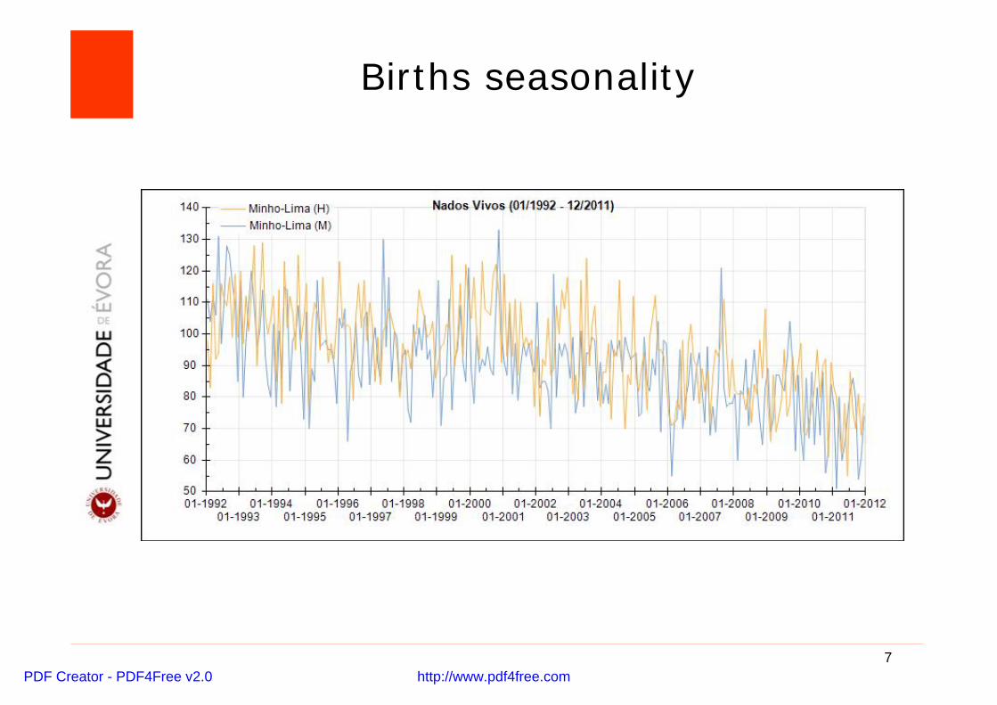
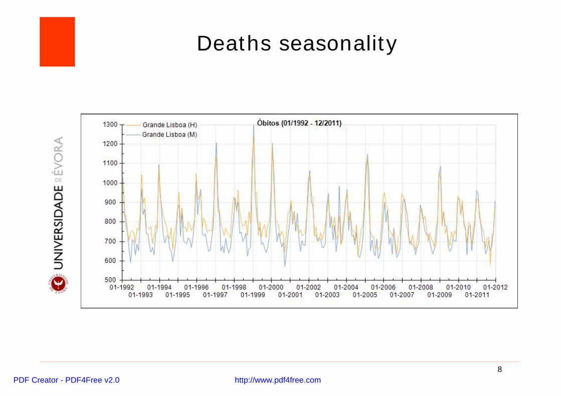
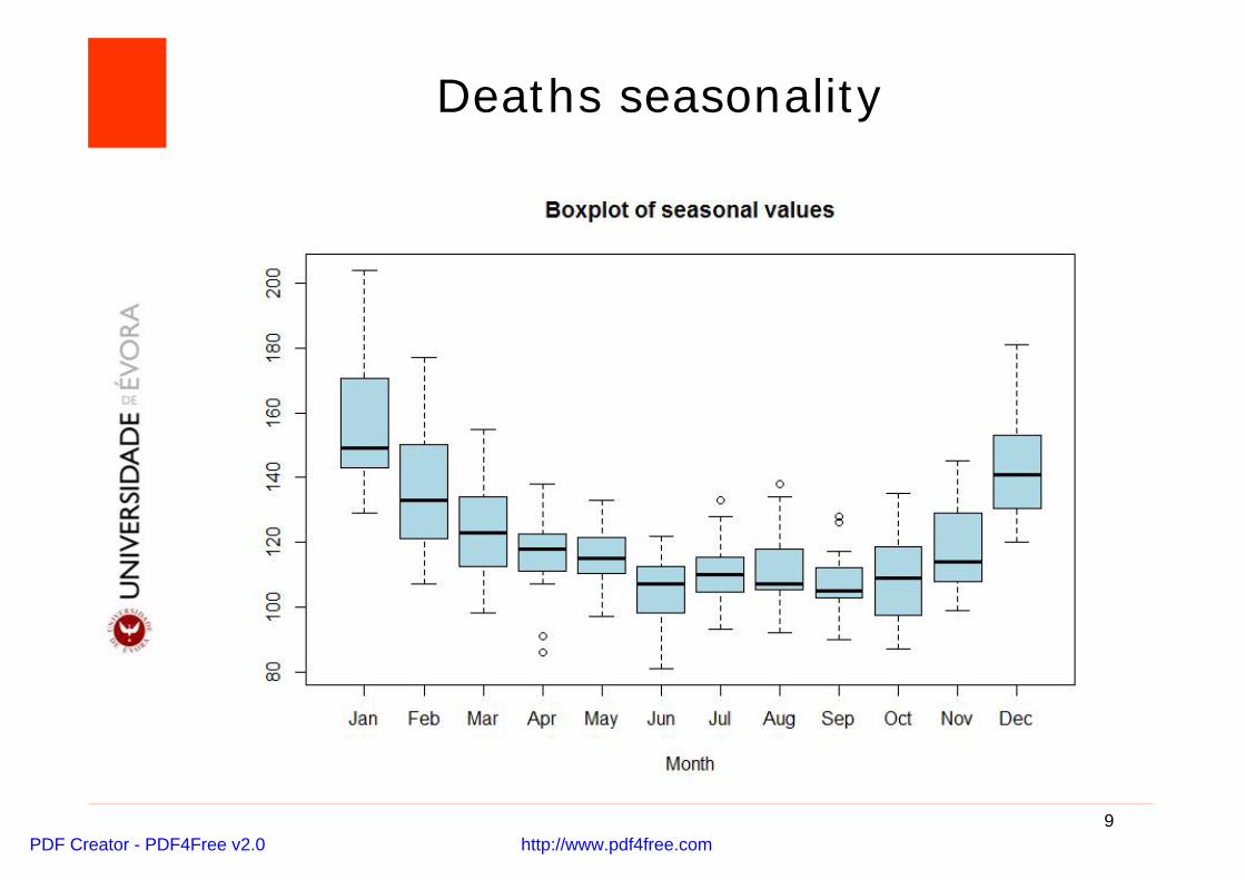
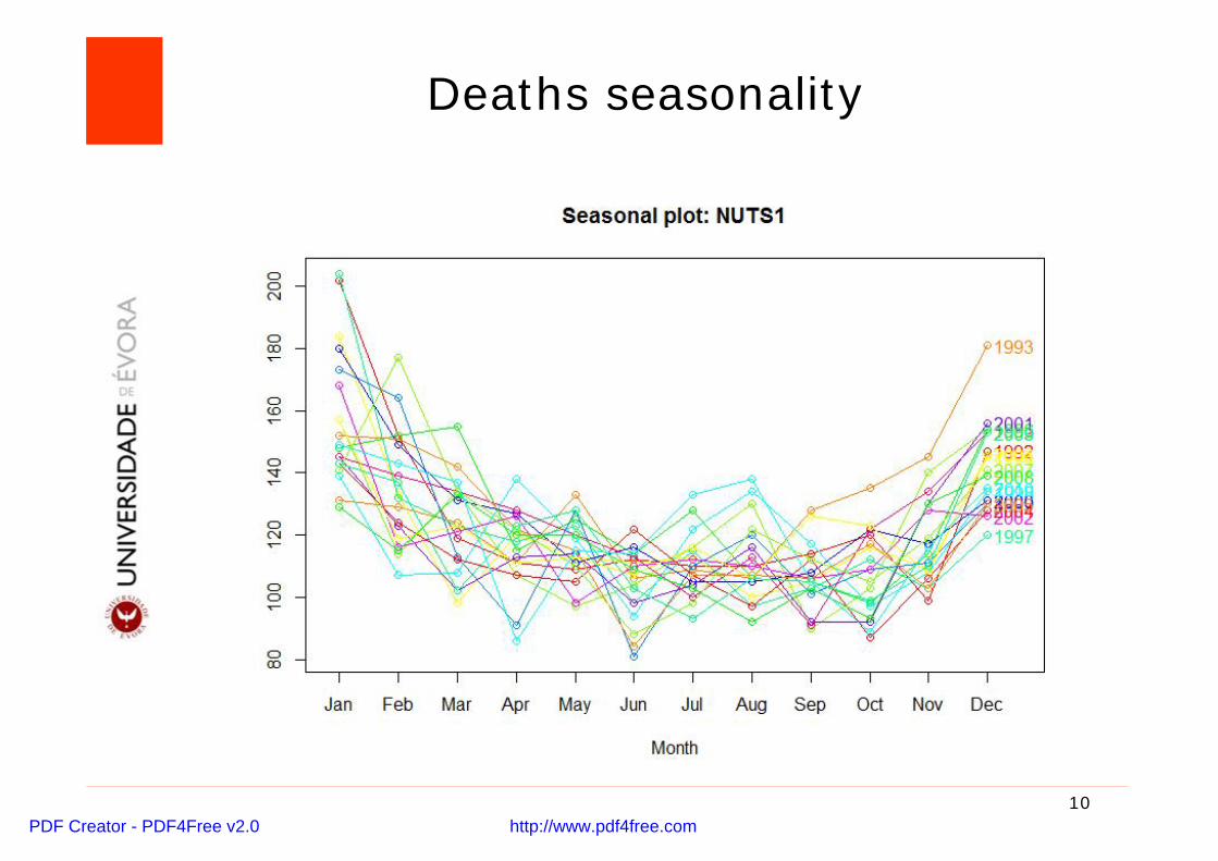
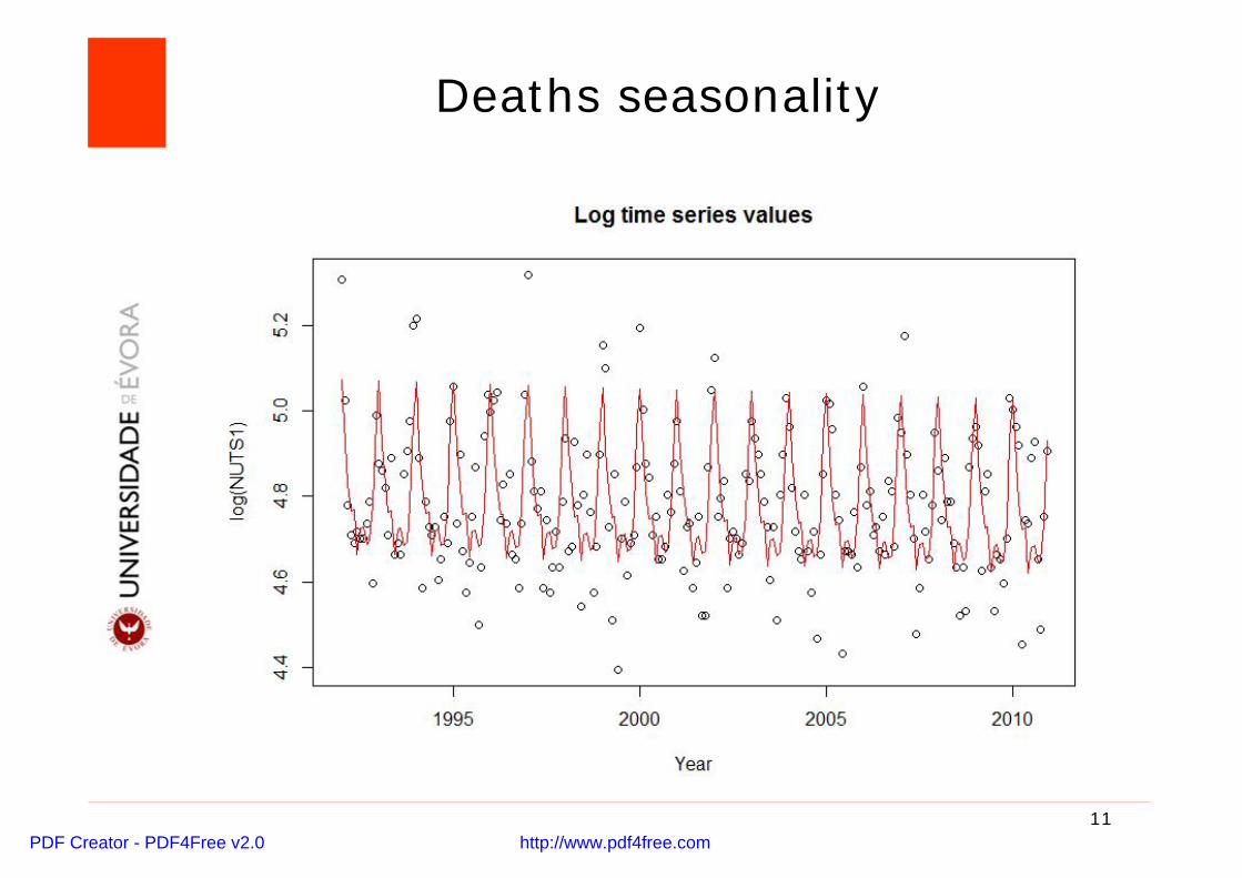
• Any time series generally consists of four components: trend,

cyclical, seasonal (additive, multiplicative) and irregular

• Births and deaths often exhibit strong seasonal patterns

• Seasonality in vital rates is the systematic, although not necessarily

regular, intra-year movement caused by the changes of the climate,

biomedical, social or demographic conditions over the calendar year

• Seasonality can be

§ deterministic (predictable)

§ or stochastic (i.e., dynamic over time)

Seasonal variation in vital rates



7

Births seasonality



8

Deaths seasonality



9

Deaths seasonality



10

Deaths seasonality



11

Deaths seasonality



12

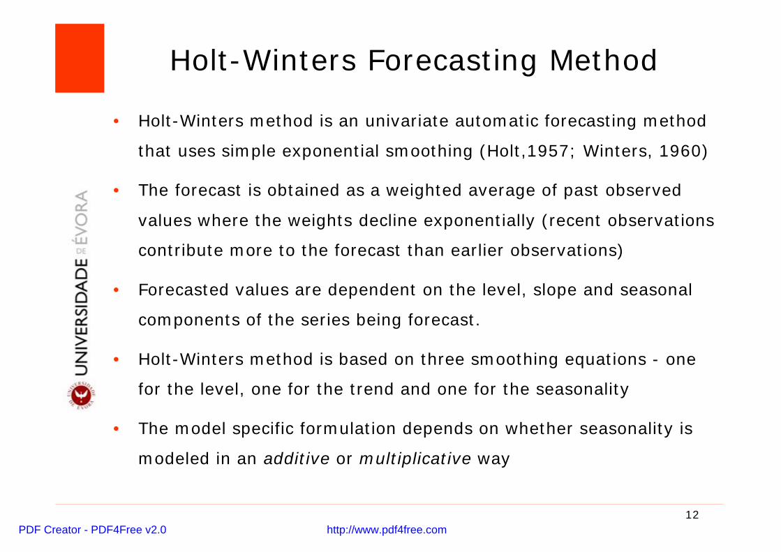
• Holt-Winters method is an univariate automatic forecasting method

that uses simple exponential smoothing (Holt,1957; Winters, 1960)

• The forecast is obtained as a weighted average of past observed

values where the weights decline exponentially (recent observations

contribute more to the forecast than earlier observations)

• Forecasted values are dependent on the level, slope and seasonal

components of the series being forecast.

• Holt-Winters method is based on three smoothing equations - one

for the level, one for the trend and one for the seasonality

• The model specific formulation depends on whether seasonality is

modeled in an additive or multiplicative way

Holt-Winters Forecasting Method



13

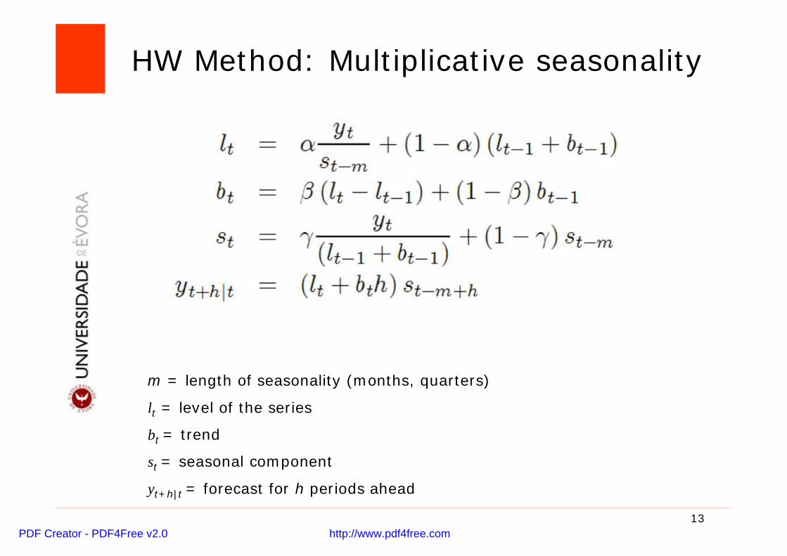
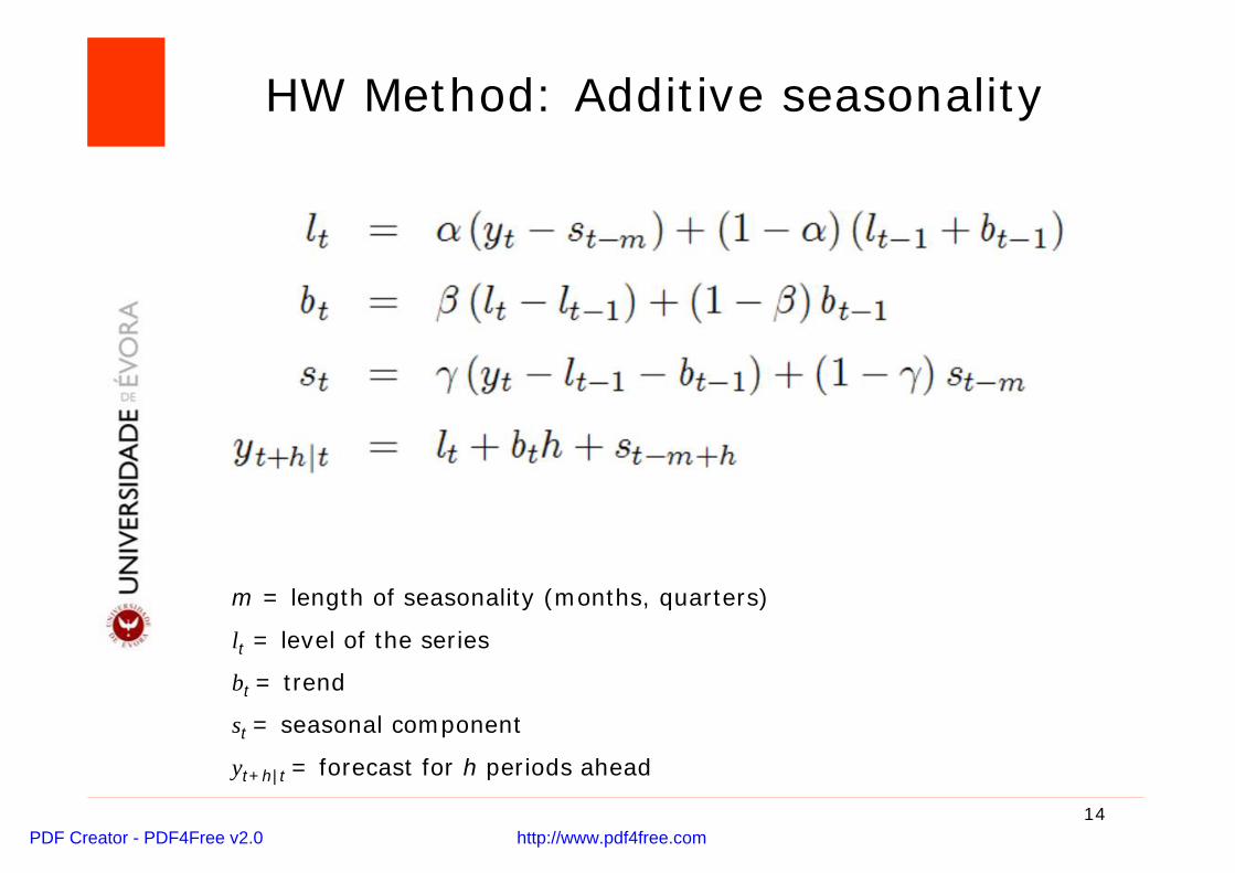
m = length of seasonality (months, quarters)

lt = level of the series

bt = trend

st = seasonal component

yt+h|t = forecast for h periods ahead

HW Method: Multiplicative seasonality



14

m = length of seasonality (months, quarters)

lt = level of the series

bt = trend

st = seasonal component

yt+h|t = forecast for h periods ahead

HW Method: Additive seasonality



15

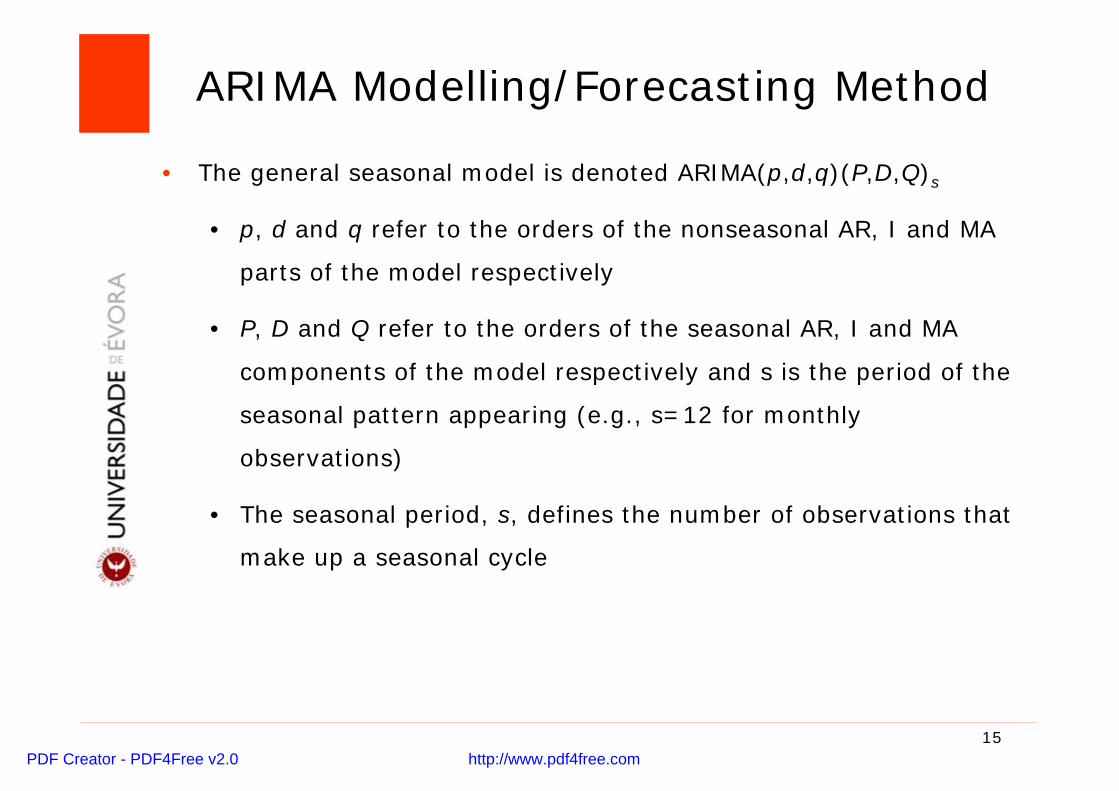
• The general seasonal model is denoted ARIMA(p,d,q)(P,D,Q)s

• p, d and q refer to the orders of the nonseasonal AR, I and MA

parts of the model respectively

• P, D and Q refer to the orders of the seasonal AR, I and MA

components of the model respectively and s is the period of the

seasonal pattern appearing (e.g., s=12 for monthly

observations)

• The seasonal period, s, defines the number of observations that

make up a seasonal cycle

ARIMA Modelling/Forecasting Method



16

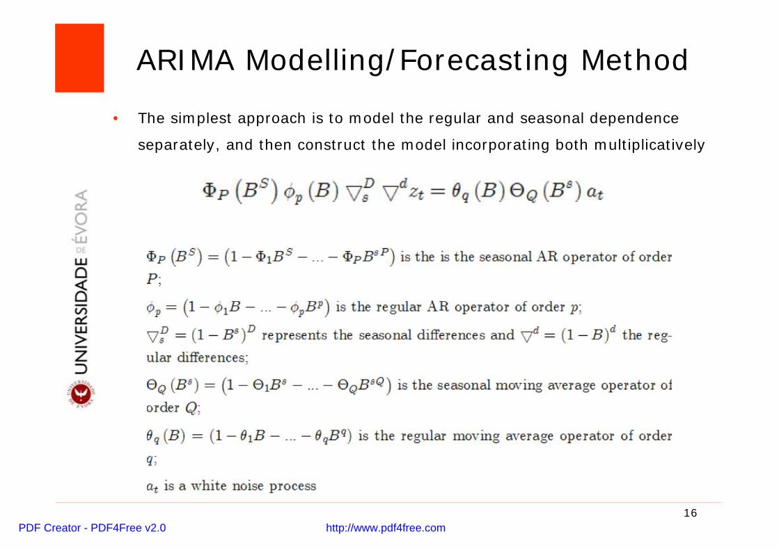
• The simplest approach is to model the regular and seasonal dependence

separately, and then construct the model incorporating both multiplicatively




17

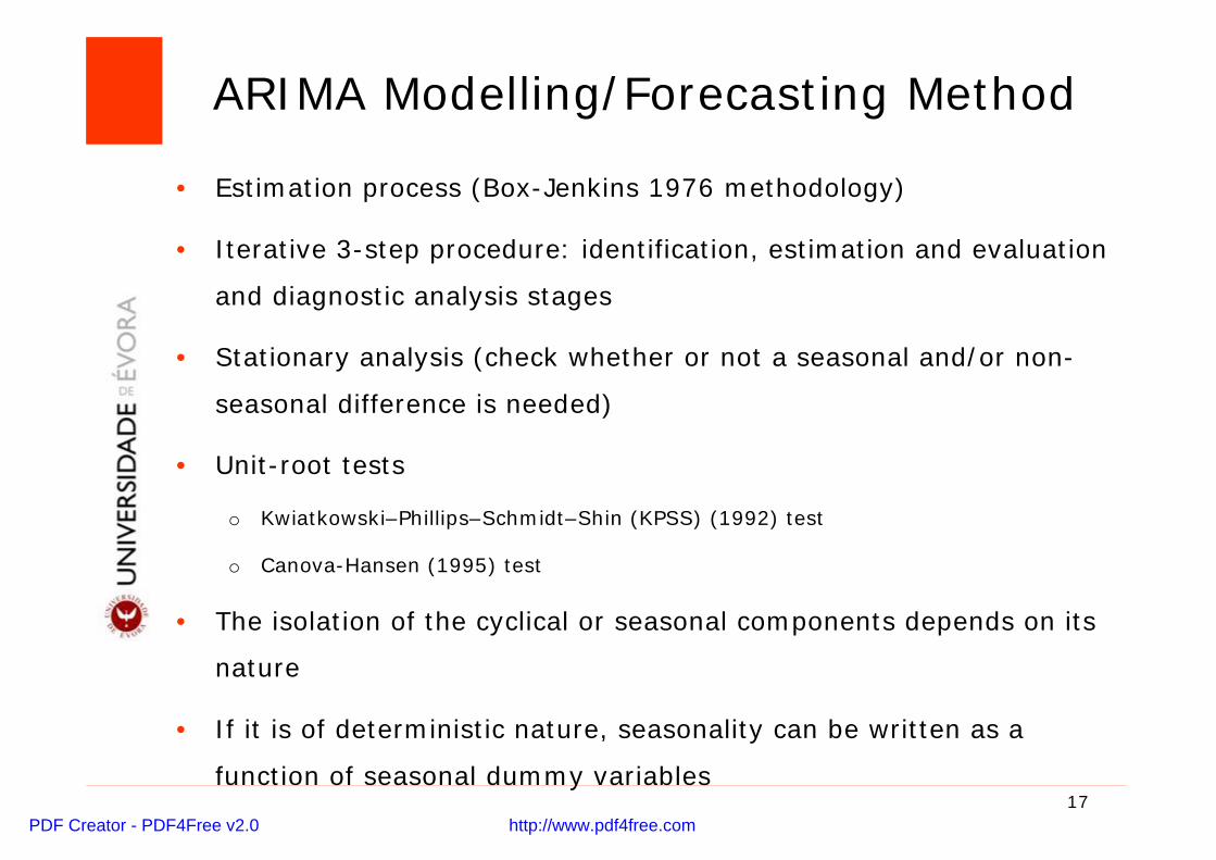
• Estimation process (Box-Jenkins 1976 methodology)

• Iterative 3-step procedure: identification, estimation and evaluation

and diagnostic analysis stages

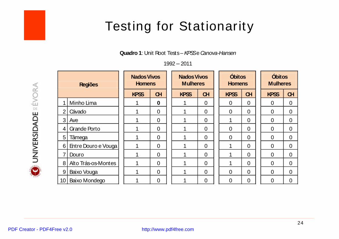
• Stationary analysis (check whether or not a seasonal and/or non-

seasonal difference is needed)

• Unit-root tests

o Kwiatkowski–Phillips–Schmidt–Shin (KPSS) (1992) test

o Canova-Hansen (1995) test

• The isolation of the cyclical or seasonal components depends on its

nature

• If it is of deterministic nature, seasonality can be written as a

function of seasonal dummy variables




18

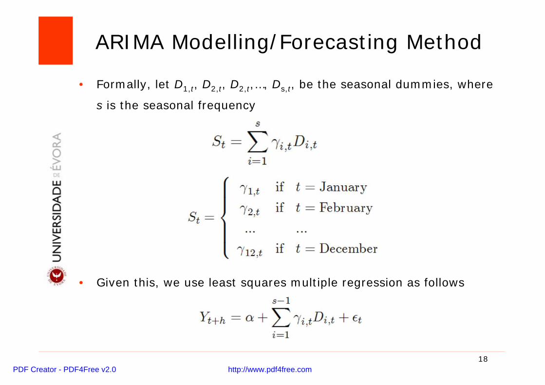
• Formally, let D1,t, D2,t, D2,t,…, Ds,t, be the seasonal dummies, where

s is the seasonal frequency

• Given this, we use least squares multiple regression as follows




19

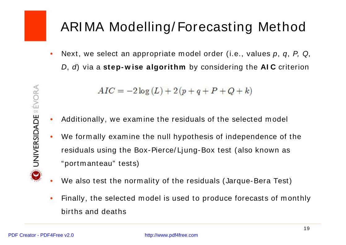
• Next, we select an appropriate model order (i.e., values p, q, P, Q,

D, d) via a step-wise algorithm by considering the AIC criterion

• Additionally, we examine the residuals of the selected model

• We formally examine the null hypothesis of independence of the

residuals using the Box-Pierce/Ljung-Box test (also known as

“portmanteau” tests)

• We also test the normality of the residuals (Jarque-Bera Test)

• Finally, the selected model is used to produce forecasts of monthly

births and deaths




20

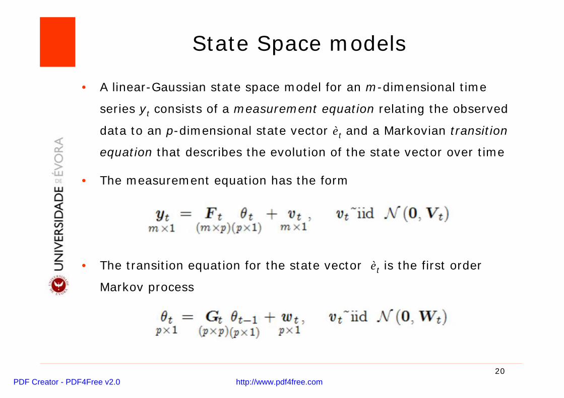
• A linear-Gaussian state space model for an m-dimensional time

series yt consists of a measurement equation relating the observed

data to an p-dimensional state vector èt and a Markovian transition

equation that describes the evolution of the state vector over time

• The measurement equation has the form

• The transition equation for the state vector èt is the first order

Markov process

State Space models



21

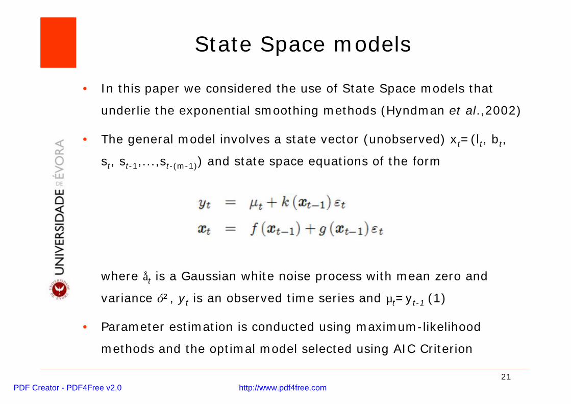
• In this paper we considered the use of State Space models that

underlie the exponential smoothing methods (Hyndman et al.,2002)

• The general model involves a state vector (unobserved) xt=(lt, bt,

st, st-1,...,st-(m-1)) and state space equations of the form

where åt is a Gaussian white noise process with mean zero and

variance ó², yt is an observed time series and µt=yt-1 (1)

• Parameter estimation is conducted using maximum-likelihood

methods and the optimal model selected using AIC Criterion

State Space models



22

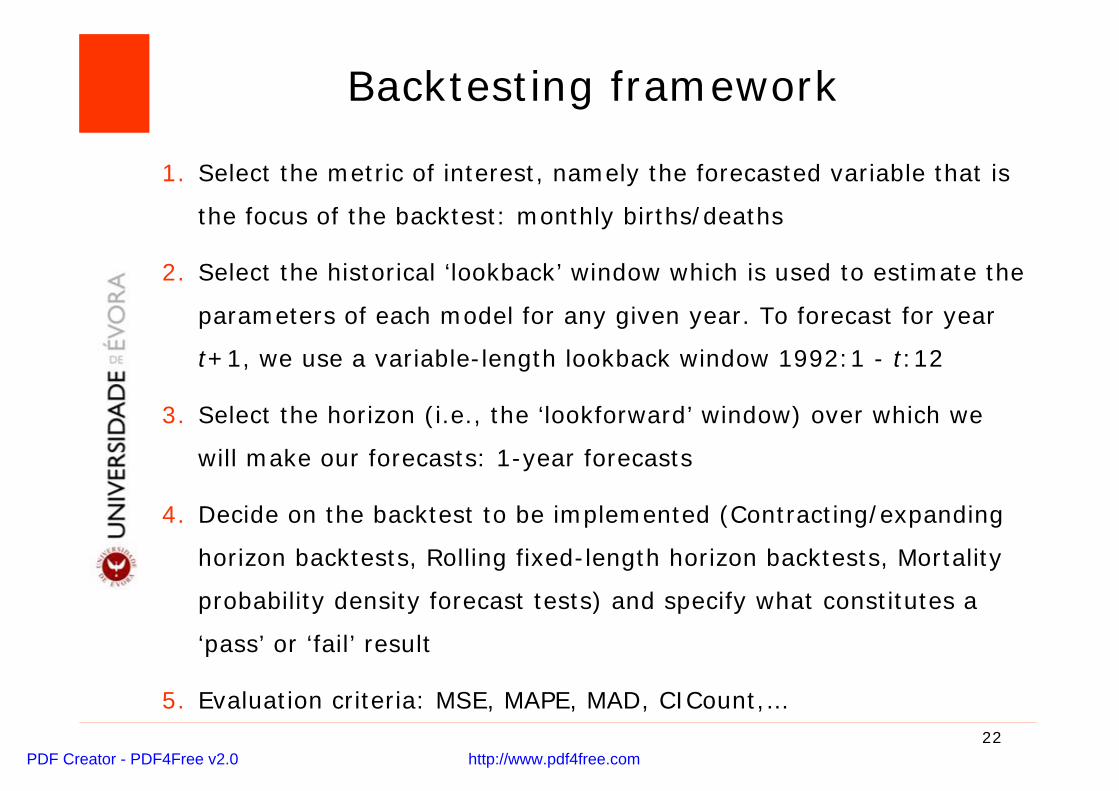
1. Select the metric of interest, namely the forecasted variable that is

the focus of the backtest: monthly births/deaths

2. Select the historical ‘lookback’ window which is used to estimate the

parameters of each model for any given year. To forecast for year

t+1, we use a variable-length lookback window 1992:1 - t:12

3. Select the horizon (i.e., the ‘lookforward’ window) over which we

will make our forecasts: 1-year forecasts

4. Decide on the backtest to be implemented (Contracting/expanding

horizon backtests, Rolling fixed-length horizon backtests, Mortality

probability density forecast tests) and specify what constitutes a

‘pass’ or ‘fail’ result

5. Evaluation criteria: MSE, MAPE, MAD, CICount,…

Backtesting framework



23

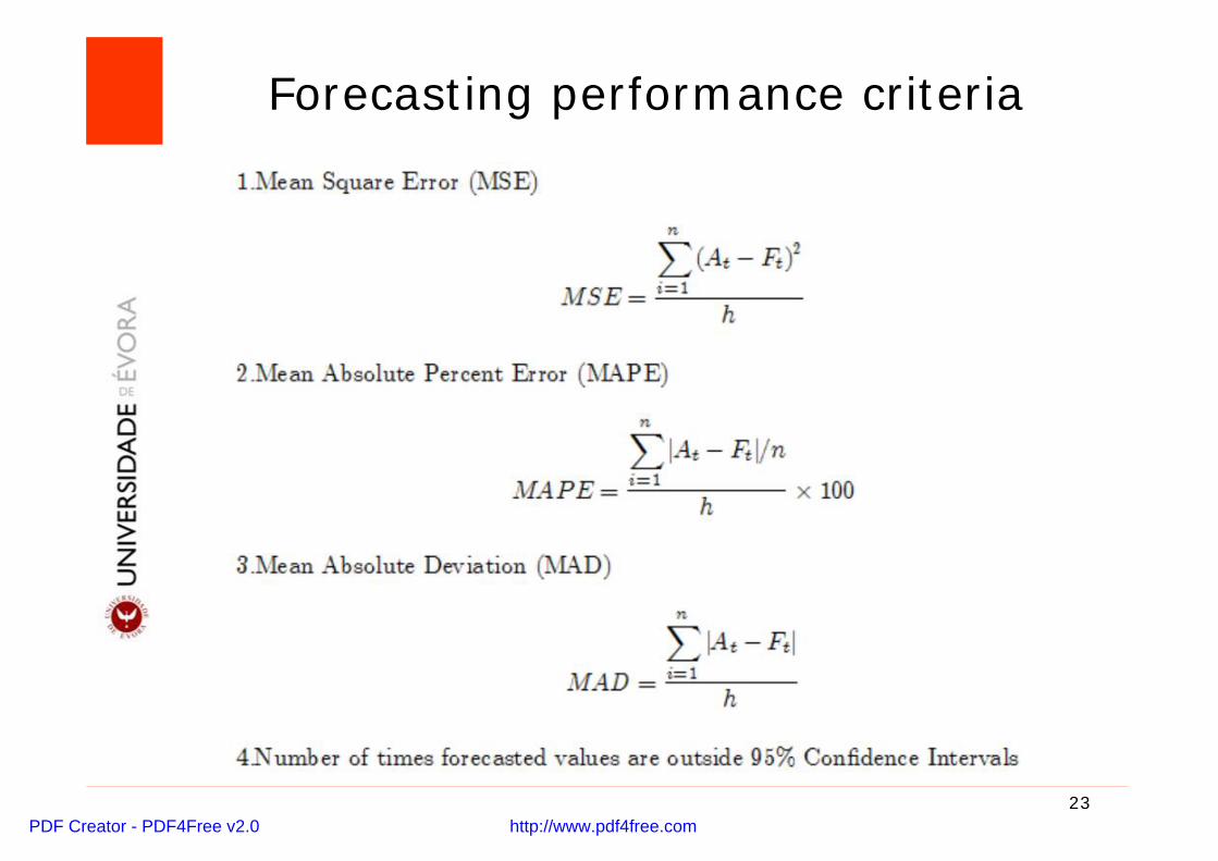
Forecasting performance criteria



24

Testing for Stationarity

Quadro 1: Unit Root Tests – KPSS e Canova-Hansen

1992 – 2011

RegiõesNados Vivos

HomensNados Vivos

MulheresÓbitos

HomensÓbitos

Mulheres

KPSS CH KPSS CH KPSS CH KPSS CH

1 Minho Lima 1 0 1 0 0 0 0 0

2 Cávado 1 0 1 0 0 0 0 0

3 Ave 1 0 1 0 1 0 0 0

4 Grande Porto 1 0 1 0 0 0 0 0

5 Tâmega 1 0 1 0 0 0 0 0

6 Entre Douro e Vouga 1 0 1 0 1 0 0 0

7 Douro 1 0 1 0 1 0 0 0

8 Alto Trás-os-Montes 1 0 1 0 1 0 0 0

9 Baixo Vouga 1 0 1 0 0 0 0 0

10 Baixo Mondego 1 0 1 0 0 0 0 0



25

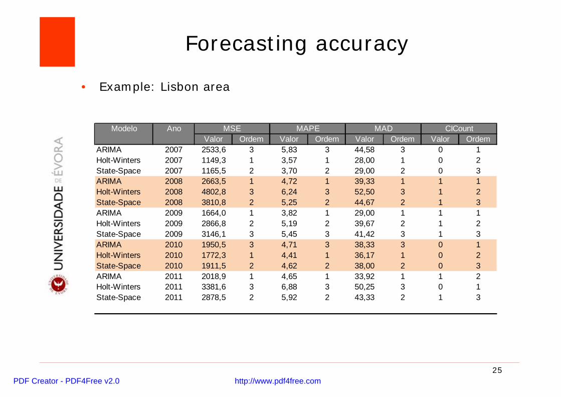
• Example: Lisbon area

Forecasting accuracy

Modelo AnoValor Ordem Valor Ordem Valor Ordem Valor Ordem

ARIMA 2007 2533,6 3 5,83 3 44,58 3 0 1Holt-Winters 2007 1149,3 1 3,57 1 28,00 1 0 2State-Space 2007 1165,5 2 3,70 2 29,00 2 0 3ARIMA 2008 2663,5 1 4,72 1 39,33 1 1 1Holt-Winters 2008 4802,8 3 6,24 3 52,50 3 1 2State-Space 2008 3810,8 2 5,25 2 44,67 2 1 3ARIMA 2009 1664,0 1 3,82 1 29,00 1 1 1Holt-Winters 2009 2866,8 2 5,19 2 39,67 2 1 2State-Space 2009 3146,1 3 5,45 3 41,42 3 1 3ARIMA 2010 1950,5 3 4,71 3 38,33 3 0 1Holt-Winters 2010 1772,3 1 4,41 1 36,17 1 0 2State-Space 2010 1911,5 2 4,62 2 38,00 2 0 3ARIMA 2011 2018,9 1 4,65 1 33,92 1 1 2Holt-Winters 2011 3381,6 3 6,88 3 50,25 3 0 1State-Space 2011 2878,5 2 5,92 2 43,33 2 1 3

MSE MAPE MAD CICount



26

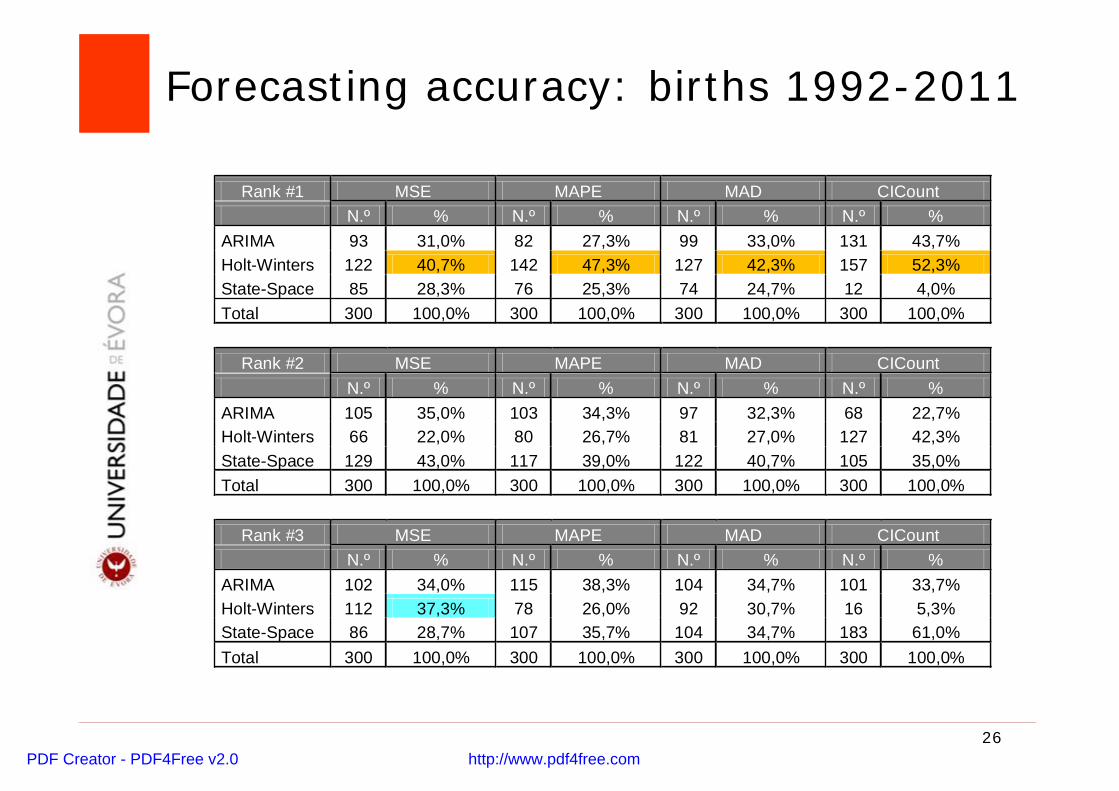
Forecasting accuracy: births 1992-2011

Rank #1 MSE MAPE MAD CICountN.º % N.º % N.º % N.º %

ARIMA 93 31,0% 82 27,3% 99 33,0% 131 43,7%Holt-Winters 122 40,7% 142 47,3% 127 42,3% 157 52,3%State-Space 85 28,3% 76 25,3% 74 24,7% 12 4,0%Total 300 100,0% 300 100,0% 300 100,0% 300 100,0%







27

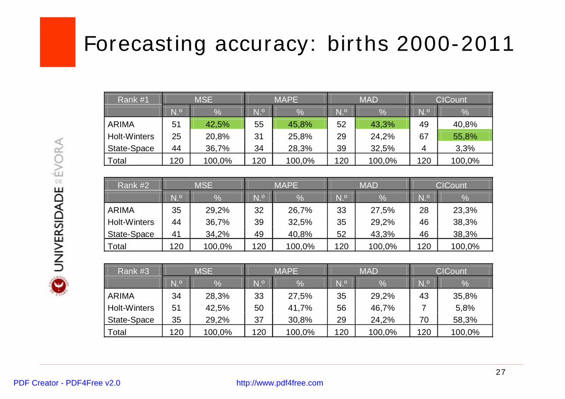
Forecasting accuracy: births 2000-2011









28

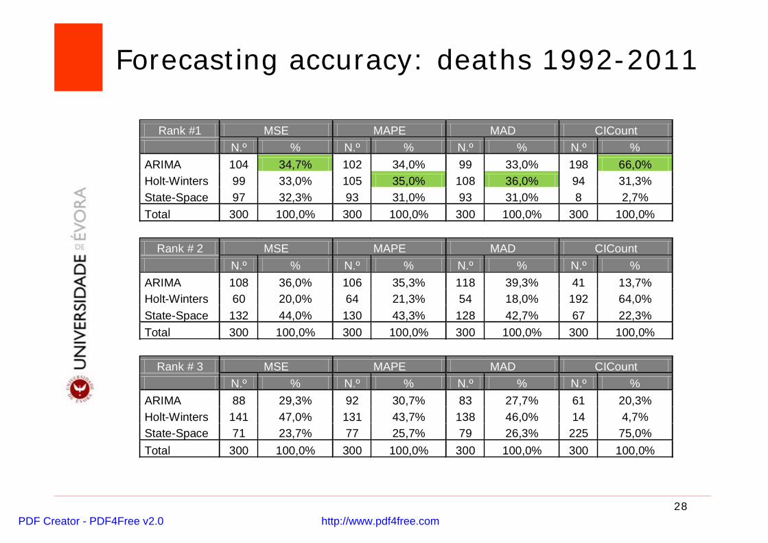
Forecasting accuracy: deaths 1992-2011



Rank # 2 MSE MAPE MAD CICountN.º % N.º % N.º % N.º %






29

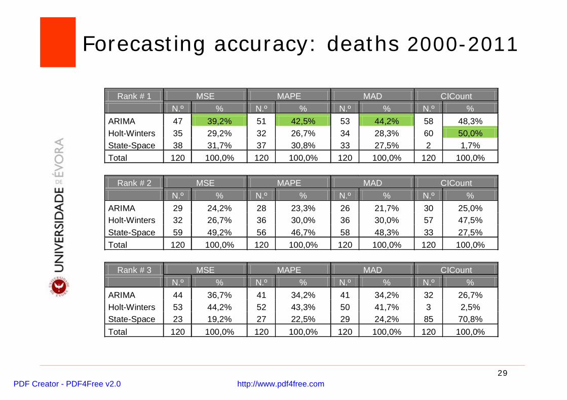
Forecasting accuracy: deaths 2000-2011









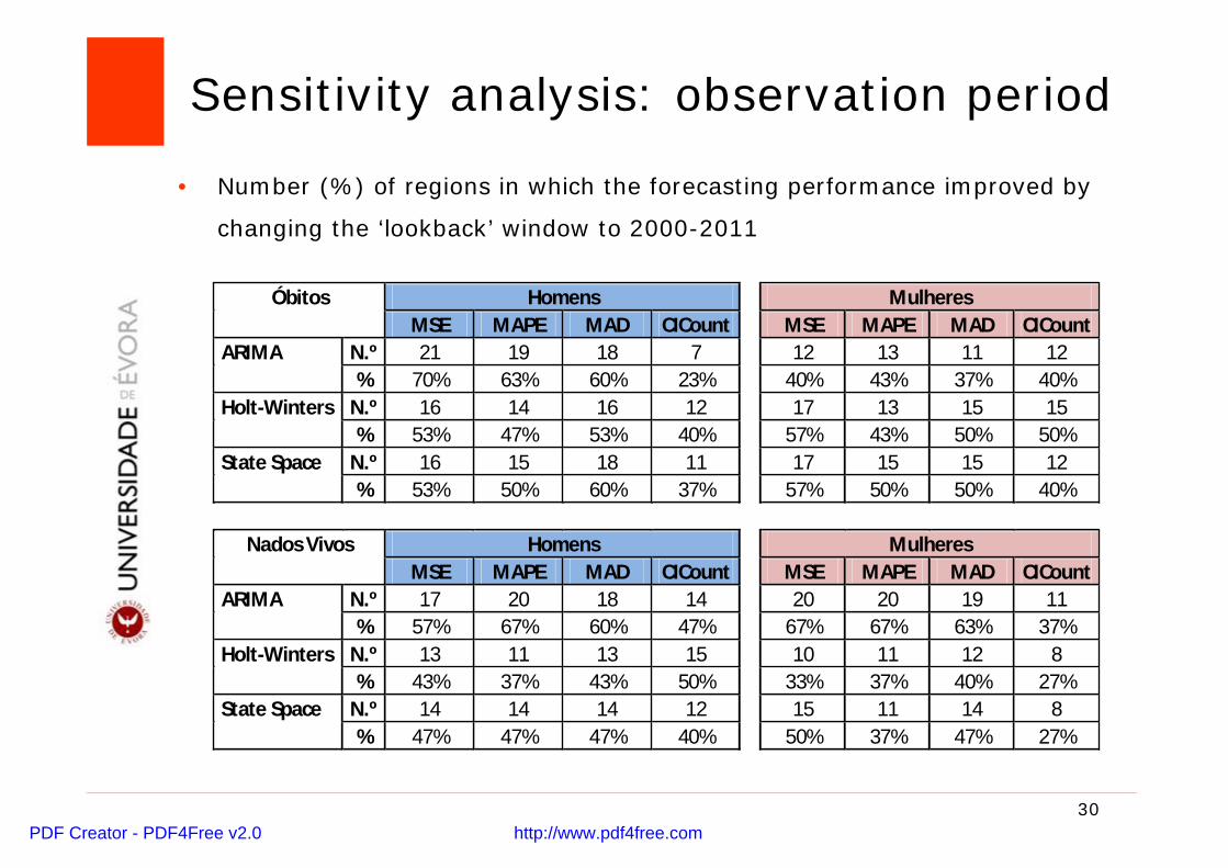
30

• Number (%) of regions in which the forecasting performance improved by

changing the ‘lookback’ window to 2000-2011

Sensitivity analysis: observation period

Óbitos Homens MulheresMSE MAPE MAD CICount MSE MAPE MAD CICount

ARIMA N.º 21 19 18 7 12 13 11 12% 70% 63% 60% 23% 40% 43% 37% 40%

Holt-Winters N.º 16 14 16 12 17 13 15 15% 53% 47% 53% 40% 57% 43% 50% 50%

State Space N.º 16 15 18 11 17 15 15 12% 53% 50% 60% 37% 57% 50% 50% 40%

Nados Vivos Homens MulheresMSE MAPE MAD CICount MSE MAPE MAD CICount

ARIMA N.º 17 20 18 14 20 20 19 11% 57% 67% 60% 47% 67% 67% 63% 37%

Holt-Winters N.º 13 11 13 15 10 11 12 8% 43% 37% 43% 50% 33% 37% 40% 27%

State Space N.º 14 14 14 12 15 11 14 8% 47% 47% 47% 40% 50% 37% 47% 27%



31

• Seasonal ARIMA models with enhanced identification, estimation

and diagnostic analysis produce, overall, the best forecasting

performance

• SARIMA models are highly flexible and accommodate most time

series patterns under study

• Holt-Winters method and State-Space models prove to be valuable

methodologies

• The models' forecasting performance improves when we reduce the

lookback window to 2000-2011

Concluding remarks



32

THANK YOUJORGE MIGUEL BRAVO

([email protected])

Eurostat/UNECE Work Session on Demographic Projections



Documents

On the use of Seasonal Forecasting Methods to model … · On the use of Seasonal Forecasting Methods to model birth and deaths data ... Cohort component method ... • Holt-Winters