Bulletin of Mathematical Biolooy Vol. 50, No. 6, pp. 579-593, 1988. Printed in Great Britain.

0092-8240/8853.00 + 0.00 Pergamon Press plc

Society for Mathematical Biology

O N T H E V A L I D I T Y O F T H E S T E A D Y STATE A S S U M P T I O N O F E N Z Y M E K I N E T I C S

LEE A. SEGEL Department of Applied Mathematics and Computer Science, The Weizmann Institute of Science, Rehovot IL-76100, Israel

By est imat ing relevant t ime scales, a simple new condi t ion can be found tha t ensures the validity of the steady state assumpt ion for a s t andard enzyme-subs t ra te reaction. The generality of the approach is demons t r a t ed by applying it to the de te rmina t ion of validity criteria for the steady state assumpt ion applied to an enzyme-subs t r a t e - inh ib i to r system,

Introduction. Virtually every biochemistry text shows how the steady state assumption can be used to approximate the kinetic equations governing an enzyme-substrate reaction and therewith to derive the informative straight- line graph of the Lineweaver-Burk plot. But texts do not present a simple clear criterion for the validity of this assumption, nor do they provide general principles that can be used to ascertain the possible use of the steady state assumption to simplify more complicated kinetic equations. This lack is not surprising, for even the research literature does not contain the required material. It is the purpose of this paper to take steps to remedy the situation. It will be seen that our approach is applicable to a variety of kinetic problems.

To set the stage, consider the enzyme-substrate reaction

k 1 k 2 E + S . -----~ C ~ E + P (1)

k - I

with governing differential equations for enzyme, substrate, enzyme-substrate complex, and product

d E / d t = - - k l E S + k _ l C + k 2 C , d S / d t = - k i E S + k ~C, (2a,b)

dC/dt = k ~ E S - k_ ~ C - kzC, dP/dt = k2C. (2c,d)

Conventional initial conditions will be assumed:

E(0)=Eo, S(0)=S o, C(0)=0, P(0)=0. (3)

There are two conservation laws:

579

580 LEE A. SEGEL

E(t) + C(t) = Eo, S( t ) + C(t) + P(t) = S o . (4a,b)

Employment of (4a) to eliminate E yields the basic mathematical problem

d S / d t = - kl (Eo - C)S + k_ ~ C, (5a)

d C / d t = kx (E o - C ) S - (k_ , + k2)C, (5b)

S(O)=S o, C(O)=O. (5c,d)

According to the steady state approximation, after an initial brief transient period it is often possible to neglect the d C / d t term in (5b). With its left side replaced by zero, (5b) becomes an algebraic equation that is easily solved to yield

C = E o S / ( K m + S), Km ==-(k_~ + k2 ) / k ~. (6a,b)

Upon substituting (6a) into (5a) one obtains

d S / d t = - k2EoS / (K . + S). (7)

It is also conventionally assumed that a negligible amount of substrate is consumed during the fast transition period, so that (7) can be solved subject to the initial condition

s(o) = So. (8)

In addition, substitution of (6a) into (2d) shows that

VmaxS V d P Vma x = k2E o. (9a,b,c) V - K m + S where = d t '

It is frequently the case in the laboratory that the initial value (just after the brief transient) of the derivative d S / d t can be estimated by observing a linear decrease in substrate over a "relatively short" time period, so that S does not decrease appreciably from S O . Then (9) can be applied to the initial reaction velocity V 0 :

1 V~ K,. + S O or Vo - - Vmax 1 + . (lOa,b)

Equation (10b) in principle permits determination of Vma ~ and K,, from a Lineweaver-Burk) plot of 1 / V o as a function of 1/S o . [It is outside the scope of this paper to consider the most efficient way to plot the data. Fersht (1985) is an excellent general reference for enzymology.]

This recapitulation of standard material allows us to pose several questions, which turn out to be closely related. (a) How can we estimate the duration of

STEADY STATE ASSUMPTION OF ENZYME KINETICS 581

the fast transition period? (b) How can we estimate how long it takes for the substrate concentration to decrease significantly? (c) For what ranges of parameters is the steady state assumption valid? (d) If the steady state assumption is regarded as a first approximation, how can a second approximation be found?

A Didactic Example. It is instructive at this point to consider a simple exactly solvable example. Consider the kinetic scheme

k 1 k 2 A ~B ~C

with the corresponding equations

d A / d t = - k i A , A(0)=Ao;

dB/d t=k lA-k2B , B(0)=B o.

C ( t ) = T - A ( t ) - B ( t ) ; T=Ao+Bo+Co, Co=C(0 ).

The elementary theory of differential equations yields the solutions

A(t)=Ao exp(-k l t ) ,

and, if k 1 ~ k2,

B(t) = B o exp(-- k2t ) kiAo k 2 - k 1 - - [exp(-- k 2 t ) - exp(-- k 1 t)].

Now C(t) can be determined from (14a). Consider the situation wherein

(11)

(12a,b)

(13a,b)

(14a,b)

(15)

(16)

k 2 ~ kl , i .e . k i 1 ~ k ? 1. (17a,b)

For a relatively short time of order k~-l, exp(_kl t ) ~ 1 so that (16) can be approximated by

B(t),,~ B o exp(-- k2t ) - (klAo/k2) [exp( - k2t ) - 1]. (18)

According to (18), B(t) rapidly approaches the value klAo/k2. For longer times exp ( - k2t ) is negligible. Now the following approximation of (16) describes the relatively slow decay of B(t) from its "initial" (after the fast transient) value kiAo/k 2 "..

B( t ) ~ (ki Ao/k2)exp(- kit ). (19)

The key observation is that from (15) and (19) it follows that

582 LEE A. SEGEL

B(t),~ (kl/k2)A(t), after the initial transient. (20)

Equation (20) would be obtained from (13a) if we assumed that dB/dt could be set equal to zero. But neither B(t) nor A(t) are in a steady state: they vary in time according to (15) and (16). Evidently dB/dt can be regarded as "very small" (after the fast transient), yielding what is often called a quasi-steady state relation (20). Such a relation holds under the conditions (17) because the time scale k 21 for a change in B(t) is so short compared to the corresponding time scale k 11 for the change in A(t). With this relation between time scales, B(t) can always completely "keep up" with--i.e, remain in a "steady-state" with respect to-- the changing concentration A(t).

The principles just enunciated are quite general. The counterpart of the quasi-steady state relation (20) between B(t) and A(t) is relation (6a) between the complex C(t) and the substrate S(t). Analogously to (17) we expect the (quasi) steady-state relation to be valid only if the time-scale t c that characterizes changes in complex concentration is small compared to the time- scale t s for substrate changes. The question is, how can we obtain estimates of t c and ts? We now turn to this matter.

Estimatin9 Time Scales. We begin with question (a). During the brief transient period the substrate concentration is not expected to change appreciably. Particularly because we want an estimate of the duration of this period (milliseconds, seconds, minutes?) we can make the approximation S = S o in (5b). This transforms (5b) into a linear equation, with the solution

C ( t ) = C [ 1 - e x p ( - 2 t ) ] , C -EoSo / (Km+So) , 2=_kl(So+Km). (21a,b,c)

Thus the complex (fast) time scale is given by t c = 2-1, i.e.

tc = [ k l ( S o + Km)] - 1 (22)

Turning to question (b), we wish to estimate how long it will take for a significant change to occur in the substrate concentration. We denote this substrate (slow) time scale by t s. We employ the characterization (Segel, 1984, p. 56)

total change in S after fast transient ts ~ max]dS/dt] after fast transient (23)

The time scale t s is an estimate of how long it takes for an appreciable change in the substrate concentration S. Formula (23) makes compensating over- estimates in providing the time for the total change in S, assuming that substrate depletion is at a maximal rate.

STEADY STATE A S S U M P T I O N O F E N Z Y M E K I N E T I C S 583

The numerator of (23) is approximately S o . Assuming the validity of the steady state assumption, we observe that the denominator is given by (7) with S = S O . Thus t s ~ S o / [ k 2 E o S o / ( K m -t- So) ], i.e.

t s = ( K m + So)/k2E o . (24)

As a numerical example we can employ data for the hydrolysis of benzoyl-L-arginine ethyl ester by trypsin where [as cited by Wong (1965)] k 1 = 4 • - l s e c -1, k _ l = 2 5 s e c -1, k2=15sec -1 so that if So=KIn, E o = 10 -3 S o then tc= 1/80 sec, ts= 133 sec.

Criteria for the Validity of the Steady State Approximation. We are now ready to obtain some simple necessary criteria for the validity of the steady state assumption. One such criterion is that the "brief transient" is indeed short compared to the time during which the substrate changes appreciably. This criterion is t c ~ t s or, from (22) and (24)

Km+S~o4~ 1 + 1 + ~ s .

In an alternative interpretation, t c ~ t s is the analog of condition (17b) for the approximation (20).

A second criterion concerns the "initial" condition (8). For this condition to be approximately valid there must be only a negligible decrease in substrate concentration during the duration t c of the brief transient. This decrease, which we denote by AS, is certainly less than the product of the time duration t c and the initial (maximal) rate of substrate consumption. '"Initial" in the previous sentence refers to the very beginning of the experiment, so that the desired rate is obtained by setting t - -0 in (5a). This yields

A oS I dS E o (26) = S Od t m a x " t c - Km+S~o"

The requirement that lAX/Sol be small compared to unity is thus expressed by

Eo e ~ 1, where e - - - (27) K m + S o"

If (27) holds then (25) holds. Thus we propose e ~ 1 as the desired simple criterion for the validity of the steady state assumption.

To check (27) let us examine the maximum velocity Vma x ~ IdP/dtlmax of the reaction. From (2d) and (21b) we see that

Vm(Calculated) c(calcula ted) ax __ - -max ( 2 8 )

VCm QssA C

584 L E E A , S E G E L

Equations (A1.1-4) of the appendix show that the dimensionless variable C / C

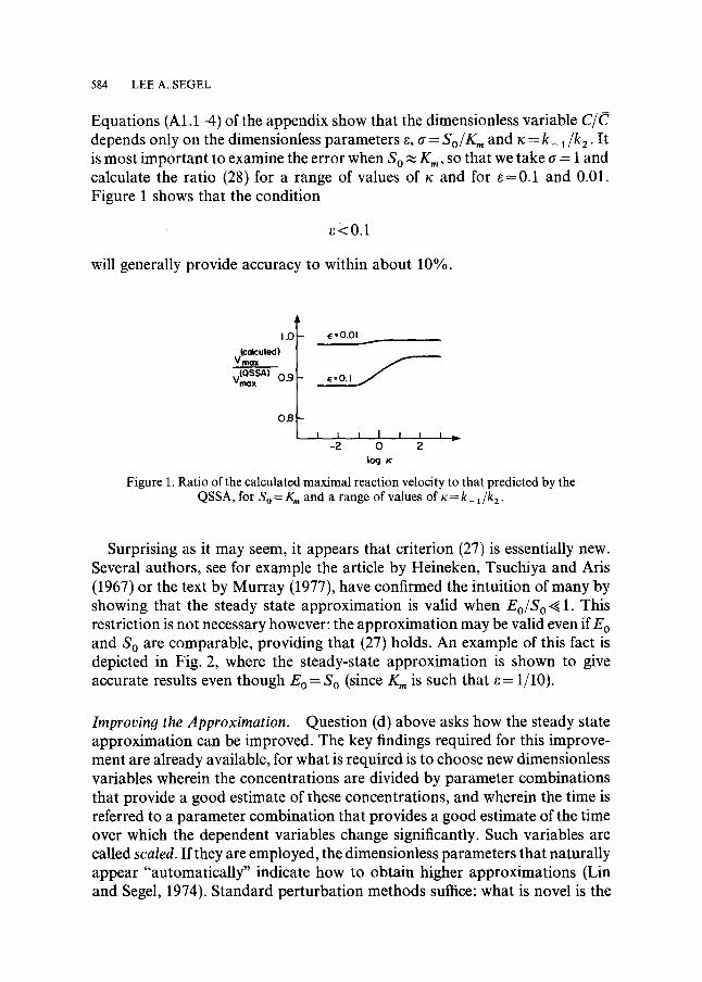
depends only on the dimensionless parameters e, a = S o / K m and x = k_ 1/k2. It is most important to examine the error when S O ~ K m, so that we take tr = 1 and calculate the ratio (28) for a range of values of x and for e=0.1 and 0.01. Figure 1 shows that the condition

~<0.1

will generally provide accuracy to within about 10%.

V~maxateuted ) I "0 t e =0'01

.(QSSA) ^ ~ / VnIw~X U'~J I

O.8[I-- 1 I t I = i t

-2 0 2 log

Figure 1. Ratio of the calculated maximal reaction velocity to that predicted by the QSSA, for S O = K~ and a range of values of K = k_ 1/k2.

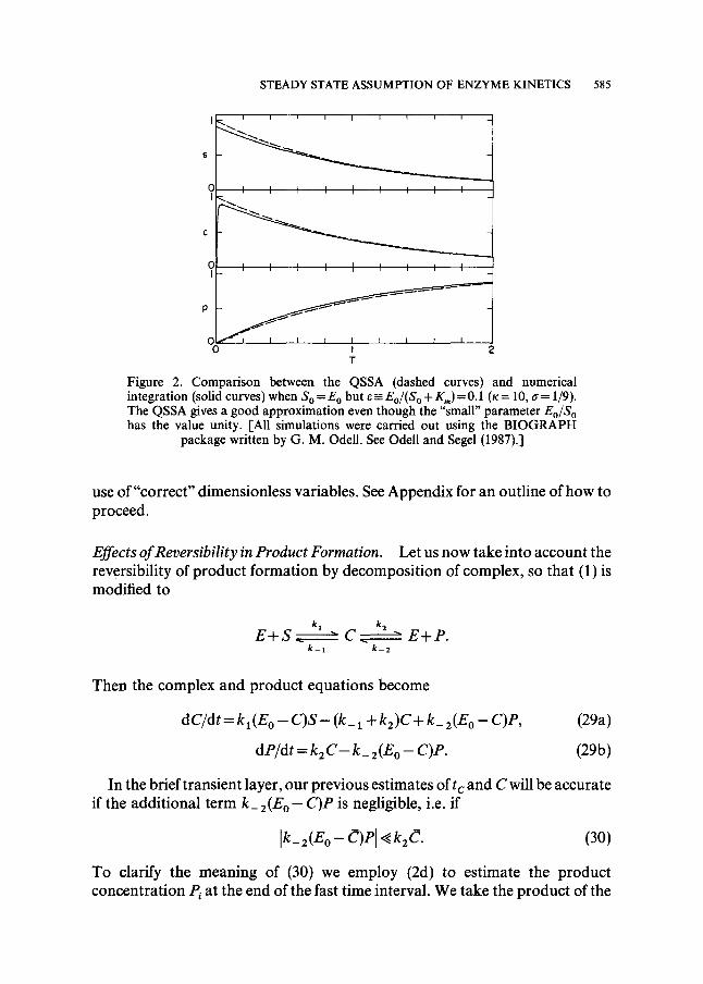
Surprising as it may seem, it appears that criterion (27) is essentially new. Several authors, see for example the article by Heineken, Tsuchiya and Aris (1967) or the text by Murray (1977), have confirmed the intuition of many by showing that the steady state approximation is valid when E o / S o ~ 1. This restriction is not necessary however: the approximation may be valid even if E o and S O are comparable, providing that (27) holds. An example of this fact is depicted in Fig. 2, where the steady-state approximation is shown to give accurate results even though E o = S O (since K m is such that e = 1/10).

Improving the Approximat ion . Question (d) above asks how the steady state approximation can be improved. The key findings required for this improve- ment are already available, for what is required is to choose new dimensionless variables wherein the concentrations are divided by parameter combinations that provide a good estimate of these concentrations, and wherein the time is referred to a parameter combination that provides a good estimate of the time over which the dependent variables change significantly. Such variables are called scaled. If they are employed, the dimensionless parameters that naturally appear "automatically" indicate how to obtain higher approximations (Lin and Segel, 1974). Standard perturbation methods suffice: what is novel is the

S T E A D Y S T A T E A S S U M P T I O N O F E N Z Y M E K I N E T I C S 5 8 5

S

I I I I I I I I I

I I I I I r I I I

0 0 I 2

T

Figure 2. Comparison between the QSSA (dashed curves) and numerical integration (solid curves) when S o = E o but ~- Eo/(S o + K,) = 0.1 (x = 10, a = 1/9). The QSSA gives a good approximation even though the "small" parameter Eo/S o has the value unity. [All simulations were carried out using the BIOGRAPH

package written by G. M. Odell. See Odell and Segel (1987).]

use of "correct" dimensionless variables. See Appendix for an outline of how to proceed.

Effects of Reversibility in Product Formation. Let us now take into account the reversibility of product formation by decomposit ion of complex, so that (1) is modified to

k~ k 2 E + S ~ -----~ C _ " E + P .

k-I k-2

Then the complex and product equations become

d C / d t = k ~ ( E o - C ) S - ( k _ x +k2)C+k_E(Eo-C)P , (29a)

dP/dt = k 2 C - k_ 2 ( E o - - C)P. (29b)

In the brief transient layer, our previous estimates of t c and C will be accurate if the additional term k_ 2 (Eo - C)P is negligible, i.e. if

Ik-2(E0 - C)P I ~ k2C. (30)

To clarify the meaning of (30) we employ (2d) to estimate the product concentration Pi at the end of the fast time interval. We take the product of the

586 LEE A. SEGEL

rate constant k2, the duration of the interval tc, and an average complex concentration C/2 yielding

P i ~ k 2 ( f f / 2 ) t c . (31)

Employing P,,~ Pi and substituting for t c and C from (22) and (21b) we find that (30) holds if

k 2 E <~ 1. (32) kl(K,.+So)

Note that even if the back reaction rate equals the forward rate, i.e. if k_ 2 = k2 ,then (32) is valid, assuming e ~ 1, since

k_ 2 k_ 2 k_2 k 1 ( K m + So) < k lK, , , - k_l + k 2 < 1. (33)

Condition (32) assures the cons is tency of the assumption that product formation may be neglected in the fast transient interval, so that in particular there is no alteration in the key requirement (27) that guarantees that A S / S o ~ 1. Lin and Segel (1974) can be consulted for instances (not expected here) where consistent approximations may nonetheless be poor. [-Note that (25) and (27) are also consistency conditions, for in deriving them we assumed the validity of (6) and (8).]

Turning to the "slow" time interval, we note that the depletion of substrate will be prolonged by reversibility while the initial rate of substrate depletion is unaltered. Thus reversibility tends to increase t s , and we have seen that moderate reversibility scarcely affects t c . As a consequence reversibility makes more likely the requirement that t c ~ t s. We conclude that our previous condition ~ ~ 1 still guarantees the validity of the steady state approximation, providing that the back reaction rate is not so large as to cause violation of (32). Of course the Michaelis-Menten formula must be generalized, for the product terms are not negligible in the slow time interval.

In case the back-reaction rate is very large, scales must be reconsidered. In the fast time interval one proceeds analogously with the irreversible case by setting S = S o in (29a). In contrast with the reversible case, the resulting equations are nonlinear and can no longer be solved explicitly. It is sufficient, however, to find the steady state solutions C and/~ (which serve as scales for C and P) and then to linearize about these solutions to determine time scales. We shall content ourselves here with this outline of how to proceed, for further details are similar to the enzyme-substrate-inhibitor case that we shall consider shortly.

STEADY STATE ASSUMPTION OF ENZYME KINETICS 587

Estimate (31) for the product concentration can be used to obtain in another way the key requirement that substrate concentration does not decrease markedly during the fast transient interval. At the end of that interval, C ~ C, P ~ k2(C/2)t c. Consequently, the conservation relation (4b) implies

S = S o - C - P ~ S o - C ( 1 + l k ) 2 2 tc/ . (34)

The requirement (S O - S)/S o < 1 yields

E~ ( 1 + 1 ) S o + K , ~ k2t c <1. (35)

But

1 1 k2 ! 1 k2tc - < 2 < (36)

2 2 kl(So+Km) So+g m 2"

Our estimates have consistently neglected factors that are order unity, so that (35) is indeed essentially equivalent to (27).

The Enzyme-Substrate-Inhibitor System. To show how the approach that we have introduced can be applied to more complicated situations, let us consider a fully competitive (irreversible) enzyme-substrate-inhibitor system:

k 1 k 2 k3 k 4 E+S=-----~C1 ,P~+E, E+I~--------~C2 ~P2+E. (37)

k - t k-3

Now the counterpart of (5a,b) is

dS/dt = - klEoS+ (klS+ k_ ~)C~ + klSC2,

dC~/dt = k l E o S - (klS+ k_ ~ + k2)C ~ - klSC2,

dI/dt = - kaEoI + (k3I+ k_ 3)C2 + k3IC~ ,

dC2/dt = k3EoI- (k3I+ k_ 3 + k4)C2 - k3IC1" (38a,b,c,d)

If we assume that both C~ and C 2 are in steady state (dC~/dt = dCE/dt = 0) we obtain the well known equations

1 1 [ K ~ ) ( , /(t),] v~S)(t ) - ~ 1 + - ~ 1

Vma x "l- g~m(/) }J' 1 1 [ K~)( S(t)'~]

V(~)(t)- V~U) 1 + ~ 1 + K(s ) ] ] . (39a,b)

588 LEE A. SEGEL

Here V ~s), V~mSa~, and K~m s~ now distinguish the abbreviations of (9) and (6) from their counterparts for the inhibitor

V a ~ _ d P 2 V~mt~x = k 4 E o ' g ~ l ) _ k _ 3 "q- k4 ( 4 0 a , b , c ) dt ' k 3

Again we ask, for what parameter domain is the steady state assumption valid? We proceed in analogy with our earlier analysis and set S = S O and I = I o in (38b) and (38d). The resulting linear equations with constant coefficients have a solution of the form

Cl( t )= Cll exp(-21t) + C12 exp( -22 t )+ C1,

C2(t) = Cx3 exp(-21t ) + C14 e x p ( - 22t) + C 2 . (41)

As expected the solutions decay exponentially. The constant concentrations attained (in this approximation) as t ~ oo are the counterparts of (21b) and provide the correct scales to use for the complex concentrations (see Appendix):

C 1 = Eoa/(a + tl + 1), C 2 = Eotl/(a + tl + 1). (42)

Here we have introduced the important dimensionless parameters

a =_ S o / K f f ), t I =Io/K~m '). (43)

The exponential factors 21 and 22 are found from the two roots of

22-2[k1(S o + Kff)) + k3(Io + K~))] + k lk3[ (S o + K f f )) (I o + K f f ) ) - S o l o ] . (44)

It is easily shown that unless o-r/,~ 1 the two roots of (44) are of the same magnitude. Roughly

21 ~ 22 ,~ k 1 (S O + K f f )) + k 3 (I o + K~"). (45)

The fast time scale t c is approximately the reciprocal of the common magnitude of 21 and 22 [compare (22)]. A formula for t c is most revealing if it is written in terms of the "individual" time scales for S and I

t~cS)- k l [So + Kf f ' ] -1 , t~c '' - k3[Io + K~')] -1 (46)

[Compare (22).] We find that

1 1 1 tc ~ ~ + t~c,-- 3 . (47)

STEADY STATE ASSUMPTION OF ENZYME KINETICS 589

On the other hand if at/,~ 1 there are two distinct time scales tic s) and ttc ~), and these can be widely separated if either t~cS)>> ttc ~) or ttcS),~ tic I).

We now can calculate the key requirement for the validity of the steady state assumption. In complete analogy with the derivation of (27) we demand small relative changes in substrate and inhibitor concentrations during the course of the fast transient period. Employing (47) we find respectively the two requirements

Eo So + K~ s) + (k3/k~) [Io + Ka']

1 and Eo

I o + K ~ ) + (k~/k3) [So + K~ s~] 41.

(48a,b)

The slow time scale for the build-up of substrate is calculated from

t s ,.~ ]So/(dS/dt)[ (49)

where dS/d t ,.~ V ~s~ is given in (39a). This yields, together with a corresponding calculation for the inhibitor,

K es~ / S O I o "~ K g ~ ( . S o I o "X ts Vmax[k +K,~ K ~ , ) tl Vmax~ "-~-'~-'{'-~ " = ~ 1 ~ - ~ + ~ / ~ , = ~ l+Km Km ) (50)

As expected, the additional requirements t c ~ ts, t c ~ t x are guaranteed by (48). In laboratory applications of the steady state hypothesis to measure kinetic

coefficients, the reaction velocity is frequently ascertained by measuring a linear decay of substrate concentration. It is advantageous to employ the simple "initial" form of (39), wherein S and / a r e replaced by S O and I o . If this is to be permitted, the inhibitor must remain close to its initial value during the time that the substrate measurements are carried out. Such is expected to be the case if the slow time scales are comparable (t s,.~ tt) but not if t s >> t~. But if the latter condition holds, all will be well if the roles of substrate and inhibitor are interchanged.

Miller and Balis (1969)found instances under which Lineweaver-Burk plots were not straight lines, but became so when the role of enzyme and inhibitor were interchanged. Rubinow and Lebowitz (1970) performed a careful theoretical analysis of the kinetics, confirming Miller and Balis' intuition as to the cause of their anomalous results. [An alternative reference is Rubinow (1975).] The parameter 3 was shown by Rubinow and Lebowitz (1970) to be the key to the analysis, where

Their development was based on the formula

I(0/Io = [s(t)/So]

(51)

(52)

590 LEE A. SEGEL

which follows at once from (39), that they correctly held to indicate that "3 is a measure of the relative fastness or slowness of the two substances." Our approach makes everything particularly transparent, for it follows from (50) that

.~ t s / t I .

That is, 6 is the ratio of the slow time scales for inhibitor and substrate.

Summary and Discussion. The most important result of this paper is the simple criterion (27) for the validity of the steady state assumption for simple enzyme-substrate reactions

E ~ o ~1" So+Kin

A number of articles [-see Segel and Slemrod (1988) for a literature survey] state that the steady state assumption is valid when Eo/S o ~ 1. This is true, but unnecessarily restrictive. As our simulations show, and as our analysis explains, the assumption can provide an excellent approximation even when E o ~ S O as long as the initial concentration of enzyme is small compared to the Michaelis constant.

Laboratory experiments are generally arranged so that E o ~ S O but there are many situations in vivo where this is not the case (Sols and Marco, 1970). Moreover, and very importantly, the formalism (1) also represents receptor (E)-ligand (S) interactions, wherein S O may very well not be large compared to E o . Thus our extension of the traditional result has biological importance.

Once the role of K m is recognized one would conjecture that the steady state assumption would also be increasingly accurate in the presence of increasing concentrations of inhibitor. This is borne out by our study of the enzyme-sub- strate-inhibitor system (37). When the forward rate constants k 1 and k 3 are comparable (and SoIo/K~)K~ ) is not too small) then the two conditions (48) collapse to a single criterion for the validity of the steady state assumption:

eo So 1.

Note that indeed the inhibitor "supplements" the Km'S. Here too the literature gives sufficient conditions for the validity of the steady state assumption, but not necessary ones: for example Rubinow (1975, p. 57) gives the requirements as Eo/S o .~ 1, k l / k 3 ~ 1, So/I o ,~ 1.

The results that we have obtained were determined by means of estimates, in terms of the parameters of the problem, of substrate and complex concentra- tions, and of the time scales for the fast initial transient and for the relatively

STEADY STATE ASSUMPTION OF ENZYME KINETICS 591

slow later period during which substrate decreases significantly. We have demonstrated (see Appendix) that with the aid of these estimates, appropriate dimensionless variables can be formed in terms of which standard singular perturbation theory provides a semi-automatic procedure for determining higher order corrections to the basic approximations.

A more thorough examination of some of the points raised here can be found in the paper of Segel and Slemrod (1988). In particular Segel and Slemrod (1988) show (i) that condition (27) is still appropriate when (3) includes the general conditions C(0) = C o, P(0) = Po; (ii) how the concept of time scales can be used to reveal the possibility of a "reverse steady state" wherein d S / d t ~ 0; (iii) how a generalized version of the steady state assumption can be used even if (27) does not hold, providing that (25) is valid.

As we indicated in treating the enzyme-substrate- inhibi tor system, our approach can be extended to a variety of kinetic problems. Another example is afforded by the paper of Frenzen and Maini (1988) who employ the concepts outlined here to the case of a two-step enzymic reaction. Some new ideas are needed when oscillatory chemical reactions are to be studied with the aid of the steady state assumption.This is because the magnitudes of the oscillating concentrations generally bear no relationship to the initial concentrations. Thoughts on this type of problem will be the subject of a future publication.

A P P E N D I X

Improving the Steady State Approximation. In exemplifying the text's brief discussion of scaled dimensionless variables let us begin with the fast transient period. From our earlier discussion it follows that S o and C are the correct concentration scales while t c is the correct time scale. We thus introduce the dimensionless scaled variables

s -S /So , c -C /C , z - t / t c , (AI.1)

with which the equations become

ds I a ~c(tc+l)-X ] dc a 1 ~zz=e - s + a + lcs-~ a + l c , ~ z = s - ~ - ~ c s - - ~ - ~ c , (A1.2a,b)

with initial conditions

s(0)= 1, c(0)=0. (A1.3a,b)

The equations contain three dimensionless parameters:

e--Eo/(So+Km), a=-So/K.,, x ~ k _ l / k 2. (A1.4)

Under our basic assumption [compare (27)] that e~ 1, the natural first approximation is to replace (A1.2a) by

ds/dz=0, i.e. s(z)-- 1. (A1.5)

592 LEE A. SEGEL

Therewith simplifying (AI.2b) we find

c(z) = 1 - e x p ( - z). (A1.6)

Equation (At.6) is simply the dimensionless version of (21a). Determination of higher approximations is in principle simply accomplished by the standard device of assuming series solutions:

S ( ~ ' ) = S ( O } ( ' / ~ ) A f ' ~ : S ( 1 } ( ~ ) " ~ - ' ' " , (~('C)=C(0)(T)-~C(1)QC)JC " " . (At.7)

Taking t c as a time scale is appropriate in the fast transient region, but not later--when we expect the steady state assumption to be valid. There the appropriate scaled dimensionless time variable is

T = t i t s . (A1.8)

Retaining the previous concentration variables we now find the dimensionless equations

d s [ _ s + ~.~_~ cs q_ _~_~[ c l ' ~___T_ (~+ 1) ( a+ 1) a x0r 1) -~

dc [ a 1 ] e -dT = (~c + 1 ) (a + 1) s - ~ cs - - ~ c . (A 1.9a,b)

The steady state assumption

( a+ 1)s c - (AI.10)

a s + 1

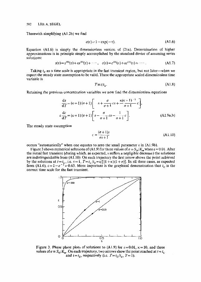
occurs "automatically" when one equates to zero the small parameter ~ in (A1.9b). Figure 3 shows numerical solutions of (A 1.9) for three values of a =-- S o / K m when ~ = 0.01. After

the initial fast transient (during which, as expected, s suffers a negligible decrease) the solutions are indistinguishable from (A 1.10)_ On each trajectory the first arrow shows the point achieved by the solutions at t = t c, i.e. z = 1, T= t c / t s = e/[(1 + K) (1 + a)]. In all three cases, as expected from (A1.6), c= l - e - -=0.63. More important is the graphical demonstration that t c is the correct time scale for the fast transient.

C o-=1

0 . 5

0 0.5 1.0 s

Figure 3. Phase plane plots of solutions to (A1.9) for e=0.01, K= 10, and three values of~ = S o / K . , . On each trajectory, two arrows show the point reached at t = t c

and t = t s , respectively (i.e. T = t c / t s , T = 1).

STEADY STATE ASSUMPTION OF ENZYME KINETICS 593

The second arrows on the trajectories show the points achieved by the solutions when t = t s, i.e. T= 1. It is thus demonstrated that t s is indeed the correct time scale for significant change in S (or s).

Higher approximations can again be found by series expansions, although "matching" methods of singular perturbation theory must be used to impose appropriate initial conditions. Segel and Slemrod (1988) provide detailed formulas for correction terms to the steady state approximation, together with a proof that the approximations are indeed valid for small e. Earlier such calculations and as well as a proof had been provided by Heineken, Tsuchiya and Aris (1967). The latter proof was less comprehensive in a certain sense [made precise by Segel and Slemrod (1988)]. More important, in the latter proof it was required that Eo/S o be small--instead of Eo/(S o + K,,).

L I T E R A T U R E

Fersht, A. 1985. Enzyme Structure and Mechanism, 2nd Edn. New York: W. F. Freeman. Frenzen, C. L. and P. K. Maini. Kinetics for a two step enzymic reaction with comparable initial

enzyme substrate ratios. Submitted for publication. Heineken, F., Tsuchiya, H. and Aris, R. 1967. "On the Mathematical Status of the Pseudo-

Steady State Hypothesis of Biochemical Kinetics." Math. Biosci. 1, 95-113. Lin, C. C. and L. A. Segel. 1974. Mathematics Applied to Deterministic Problems in the Natural

Sciences. New York: MacMillan. Miller, H. K. and M. E. Balis. 1969. Glutaminase Activity of L-asparagine amidohydrolase."

Biochem. Pharmacol. 18, 2225-2232. Murray, J. D. 1977. Lectures on Nonlinear Differential Equation Models in Biology. London:

Clarendon Press. Odell, G. M. and L. A. Segel. 1987. BIOGRAPH. A Graphical Simulation Package With

Exercises. To Accompany Lee A. Segers "Modeling Dynamic Phenomenon in Molecular and Cellular Biology." Cambridge: Cambridge University Press.

Rubinow, S. I. 1975. Introduction to Mathematical Biology. New York: Wiley. - - and J. L. Lebowitz. 1970. "Time-Dependent Michaelis-Menten Kinetics for an

Enzyme-Substrate-Inhibitor System." J. Am. Chem. Soc. 92, 3888-3893. Segel, L. A. 1984. Modeling Dynamic Phenomena in Molecular and Cellular Biology. Cambridge:

Cambridge University Press. - - and M. Slemrod. 1988. "The Quasi-Steady State Assumption: A Case Study in

Perturbation." S l A M Review, in press. Sols, A. and Marco, R. 1970. "Concentrations of Metabolites and Binding Sites. Implications in

Metabolic Regulation." In Current Topics in Cellular Regulation, Vol. 2. New York: Academic Press.

Wong, J. T.-F. 1965. "On the Steady-State Method of Enzyme Kinetics." J. Am. Chem. Soc. 87, 1788-1793.

Rece ived 29 M a r c h 1988