Embed Size (px)
Citation preview
Paper prepared for"The 3rd Conference of the European Research Network on Divorce"
University of Cologne, GermanyDecember 2nd - 4th 2004
On the variation of divorce risks in Europe: a meta-analysis
Michael Wagnerand
Bernd Weiss
6th December 2004
Research Institute for SociologyUniversity of Cologne
Greinstr. 250 939 Cologne
[email protected]@wiso.uni-koeln.de
Contents
1. Introduction 3
2. Divorce risks 3
3. Divorce risks and the societal context: some hypotheses 43.1. Modernization . . . . . . . . . . . . . . . . . . . . . . . . . . . . . . . . . . . 53.2. Marriage culture: Barriers to divorce . . . . . . . . . . . . . . . . . . . . . . . 6
4. Data and methods 64.1. Literature retrieval and sample description . . . . . . . . . . . . . . . . . . . 74.2. Levels of Analysis . . . . . . . . . . . . . . . . . . . . . . . . . . . . . . . . . . 84.3. Statistical methods . . . . . . . . . . . . . . . . . . . . . . . . . . . . . . . . . 9
4.3.1. Synthesis . . . . . . . . . . . . . . . . . . . . . . . . . . . . . . . . . . . 114.3.2. Testing for homogeneity of effect sizes . . . . . . . . . . . . . . . . . . 124.3.3. Estimation of weights . . . . . . . . . . . . . . . . . . . . . . . . . . . 13
5. Results 135.1. Country-specific divorce risks and their European summaries . . . . . . . . 13
5.1.1. Premarital cohabitation . . . . . . . . . . . . . . . . . . . . . . . . . . 135.1.2. Age at Marriage . . . . . . . . . . . . . . . . . . . . . . . . . . . . . . . 145.1.3. Experiences with parental divorce . . . . . . . . . . . . . . . . . . . . 175.1.4. Presence of children . . . . . . . . . . . . . . . . . . . . . . . . . . . . 175.1.5. Resources . . . . . . . . . . . . . . . . . . . . . . . . . . . . . . . . . . 18
5.2. Publication characteristics and divorce risks . . . . . . . . . . . . . . . . . . . 235.3. Context variables and divorce risks . . . . . . . . . . . . . . . . . . . . . . . . 25
5.3.1. Macro-level indicators . . . . . . . . . . . . . . . . . . . . . . . . . . . 255.3.2. Results for heterogeneity analysis by macro-level indicators . . . . . 27
6. Discussion 31
A. Forest plots 36
2
1. Introduction
The aim of this paper is to summarize European research on divorce risks. More precisely,we will examine how much divorce risks vary between European countries and whethersuch variations can be explained by country-specific macro-level factors. Are there anymeaningful differences in the divorce risks between European countries?
We perform a meta-analysis of 120 publications from European longitudinal divorcestudies that include empirical results from 21 European countries. This study is based ontwo earlier papers on the results of German divorce research (Wagner and Weiß, 2003a,2004) and its first extension towards an European level (Wagner and Weiß, 2003b). Here,we will proceed in two ways. First, we propose an improved conceptualization of macro-level factors. Secondly, we extend the spectrum of variables as we include not only in-dicators of the information level and marital investments but also of the partners’ socialresources and their divorce experience. Thirdly, we look more closely at the problem thateffect sizes are likely to differ according to the inclusion of control variables.
In a first step, we describe the elements of a divorce model and we characterize impor-tant divorce risks. Secondly, we specify hypotheses on the differences of divorce risksbetween European countries. Thirdly, we inform about our data and methods. Fourthly,we describe the European pattern of divorce risks and we discuss the problem whetherthe variation of divorce risks is a result of different methods applied. The last step isconcerned with the question to what extent macro variables account for the variability ofdivorce risks across European countries.
2. Divorce risks1
Most theories that are applied to explain divorce risks are formulated at the micro-levelof the individual or at the meso-level of the marital dyad. Central to microeconomic andexchange theories are the costs and gains marriage partners perceive from the actual mar-riage and from alternative options. It is assumed that individuals have several optionswith different expected costs and gains, individuals have at their commands certain re-sources (e.g. time for partner search) and that these resources are scarce.
Exchange theory assumes that individuals achieve their aims through an exchange ofmaterial and immaterial resources in that way that rewards are maximized and costs areminimized. The exchange of resources is regulated by norms of reciprocity and justicewhich enhance the progression of trust and commitment (Sabatelli and Shehan, 1993).Exchange theory has been applied to marital stability by Levinger (1965, 1982) and Lewisand Spanier (1979). It is hypothesized that marital stability depends on the quality ofrelationship, on the alternatives to the existing marriage, and on external social barriers whichare opposed to divorce. Marital quality is attributed to social and personal resources, tosatisfaction with the life style, and to rewards of spousal interaction. In accordance with themicroeconomic theory, several authors also emphasized the role of marital investmentsbecause they increase the costs of divorce. Couples break up if the quality of relationshipfalls below the aspiration level and if the expected gain from alternatives (for example a
1Parts of this section have already been published in Wagner and Weiß (2002, 2003b).
3

relationship with another partner) exceeds the costs of divorce.Based on the studies of Gary S. Becker, the microeconomic theory of the family suits
exchange theory in many aspects. It assumes persons to organize their household in sucha way that the utility of commodities is maximized. If the collective utility of marriage isless than the expected utility of the alternatives, the marriage will be divorced. Amongother things, the rewards of marriage depend on the mode of division of labor, investmentsin marital capital, and the "partner-match". Because microeconomic theory gives up theneoclassical fiction of a perfect market, conceptions like level of information and subjectiveinsecurity are implemented into the theory. Search costs arise because individuals needinformation about potential spouses. At the time of marriage not all attributes of thepartners are known (Hill and Kopp, 1995).
Very little theoretical research deals with the question whether the explanatory powerof the well-established divorce models depends on the wider societal context. Is the im-portance of certain determinants of divorce related to macro-level factors? In the follow-ing, we will present some hypotheses on how this societal context could affect divorcerisks.
We confine our analysis to four theoretical constructs which will be explored in a com-parative meta-analysis across European countries: premarital information level, maritalinvestments, personal resources and divorce experiences.
3. Divorce risks and the societal context: somehypotheses
As it is not reasonable to develop different theories of marital stability for different coun-tries it may well be that the strength of the proposed relationships between the variablesof a divorce model or the importance of certain predictors vary according to the widersocietal context. In empirical research, variation in societal context can be realized bya historical or a cross-national design. Historical studies are not only concerned withtrends in divorce rates but also with historical changes of different kinds of divorce risks(e.g. Wagner, 1997; Wolfinger, 1996).
There are three types of comparative studies. First, there are studies at the aggregatelevel that correlate national divorce rates with other aggregate statistics (e.g. Trent andSouth, 1989). Such studies have been critized for their missing correspondence to anaction-oriented explanation. Secondly, there are a number of new studies that comparemarriage behavior or divorce risks with micro data between single countries (Brüderland Diekmann, 1997; Diekmann and Schmidheiny, 2002). As these studies do not groupthe countries according to theoretical criteria they are usually descriptive without testingmacro-micro hypotheses.
Thirdly, as Gerhards and Hölscher (2003) argue countries are not very meaningful unitsof sociological analysis. Rather the unit "country" should be replaced by dimensionswhich are assumed to affect processes at the meso or micro level. The authors developthree dimensions: the level of modernization, cultural or religious orientations and thetype of family policy and welfare.
Another way of replacing countries by more theoretically validated constructs is the
4
construction of typologies. Welfare state typologies – like those from Esping-Andersen –have been applied to understand patterns of partner choice (Blossfeld and Müller, 2002),normative orientations toward women’s employment (Künzler et al., 1999) or the eco-nomic consequences of separations (Uunk and Kalmijn, 2002). However, many of thesestudies revealed that the explanatory power of such welfare typologies is very restricted.
In the following, we concentrate on two macro level factors: the degree of socioeco-nomic development or the modernization level and a more cultural factor that capturesthe strength of the marriage as an institution or of marital norms. The latter should in-dicate how much a society can be characterized by a more traditional marriage culture.Despite the fact that many scholars have criticized modernization theory because the con-cept "modernization" is vague and predictions of this theory have been falsified, it is stillan important question whether the socioeconomic development of a country, like the liv-ing standard, the expansion of the educational system or an increase in the labor marketchances of women affect divorce risks.
3.1. Modernization
If the level of modernization is high, individuals stay longer in the educational systemand marry relatively late. So far as the "institution effects hypothesis" holds, marriageand family formation are highly incompatible with educational enrollment and a careerorientation of women, early marriages should be especially "dysfunctional". From theperspective of the differentiation hypothesis, modernized countries are characterized byheterogenous marriage markets that require a longer partner search. Also for this reason,marriage age should matter more in these countries: The higher the level of moderniza-tion the stronger marriage age reduces the divorce risk.
The same is true in the case of cohabitation if we take cohabitation as an indicator ofhow much information about the partner is available before marriage. The higher thelevel of modernization the stronger cohabitation should reduce the divorce rate. It isknown that it is important to control for selectivity processes, because those who do notcohabit before marriage might be very reluctant to divorce. Selectivity and modernizationare likely to be linked in a U-shaped manner (Dourleijn and Liefbroer, 2003).
Research has clearly demonstrated that the presence of children is an important mari-tal investment that lowers the divorce rate. It is still not clear to what extent economic,social or emotional factors account for the fact that children born in the marriage increasemarital stability. Very little comparative research on children’s influence on marital sta-bility has been undertaken. Given economic factors play a role and countries differ withrespect to the effect of children on marital stability, modernization theory would arguethat the economic risks of living as a single parent decrease with a rising living standard,gainful employment of women and more economic independence of women. From thatperspective, the divorce risk associated with the presence of children should be lower incountries that are highly modernized. However, insofar as children increase the costs ofa divorce because parents do not want that their children grow up only with one parent,no correlation with the modernization level can be expected.
Whether the transmission effect is related to the socioeconomic development level ofthe society depends on the mechanisms that are responsible for the higher divorce risk of
5
people whose parents have been divorced. If parental divorce leads to economic and ed-ucational disadvantages for the children that in turn affect their own marriage negatively,the transmission effect should be stronger in countries with a low modernization level.
The higher the level of modernization the higher the general level of resources amongthe members of the society. In that case, resources should play a lesser role for an expla-nation of divorce. For example, a partner is less dependent on the resources of anotherpartner if many others potential partners exist with a similar level of resources.
3.2. Marriage culture: Barriers to divorce
In a country where marriage is highly institutionalized premarital cohabitors are a moreselective group than in societies that are characterized by a weak institutionalization ofmarriage. In the latter case we expect cohabitation to be less selective and to be lessstrongly correlated with the divorce risk.
If marriage as an institution is less important and if many marriages get divorced, onecan assume that a "divorce culture" has emerged that also facilitates parenthood after aseparation. For that reason, it can be stated that the effect of children on marital stabilityshould be stronger with higher divorce barriers.
If a marriage is divorced despite there are children, the "pressure" to divorce shouldbe very high. Therefore, children might suffer much more under such conditions. Incountries with high barriers to divorce only very devasted marriages get divorced whichmeans that children from such marriages have to bear a parental marriage which is es-pecially destructive. If barriers to divorce are low, the experience of a divorce should beless stigmatizing and divorce becomes less deviant. This should result in a less seriouseffect of the parental divorce on the stability of children’s marriage. The transmissionhypothesis should hold less in case of low divorce barriers.
Resources should play a greater role in a social context in which divorce barriers arehigh. The higher the costs of a divorce the more resources are necessary to overcomethe divorce barriers. Moreover, in a high-divorce country more alternative partners areavailable which should reduce the role of resources that a given marriage partner canprovide. Blossfeld et al. (1995) demonstrated that the educational attainment of womenhas its "liberating effect" mostly in countries with a high overall level of divorce (such asItaly). The same should be true with respect to women’s employment status.
4. Data and methods
Meta-Analysis is a technique that covers the whole research process. We apply a fivestage-model proposed by Cooper (1982): (1) research question, (2) literature retrieval, (3)data coding and data entry, (4) data analysis and (5) presentation of results (for details seeWagner and Weiß, 2003b).
If a meta-analysis about divorce risks in Europe is to be conducted, it is necessary toclarify which countries have to be included into the study. The countries considered hereare the 18 countries of the European Economic Area (EEA)2; the candidate countries for
2The European Economic Area (EEA) exists since 1994 and includes the 15 countries of the European
6
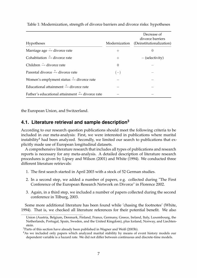
Table 1: Modernization, strength of divorce barriers and divorce risks: hypotheses
Decrease ofdivorce barriers
Hypotheses Modernization (Deinstitutionalization)
Marriage age −−→ divorce rate + 0
Cohabitation +−→ divorce rate + − (selectivity)
Children −−→ divorce rate 0 −
Parental divorce +−→ divorce rate (−) −
Women’s emplyment status +−→ divorce rate − −
Educational attainment +−→ divorce rate − −
Father’s educational attainment +−→ divorce rate − −
the European Union, and Switzerland.
4.1. Literature retrieval and sample description3
According to our research question publications should meet the following criteria to beincluded in our meta-analysis: First, we were interested in publications where maritalinstability4 had been analyzed. Secondly, we limited our search to publications that ex-plicitly made use of European longitudinal datasets.
A comprehensive literature research that includes all types of publications and researchreports is necessary for any meta-analysis. A detailed description of literature researchprocedures is given by Lipsey and Wilson (2001) and White (1994). We conducted threedifferent literature retrievals:
1. The first search started in April 2003 with a stock of 52 German studies.
2. In a second step, we added a number of papers, e.g. collected during "The FirstConference of the European Research Network on Divorce" in Florence 2002.
3. Again, in a third step, we included a number of papers collected during the secondconference in Tilburg, 2003.
Some more additional literature has been found while ’chasing the footnotes’ (White,1994). That is, we checked all literature references for their potential benefit. We also
Union (Austria, Belgium, Denmark, Finland, France, Germany, Greece, Ireland, Italy, Luxembourg, theNetherlands, Portugal, Spain, Sweden, and the United Kingdom), plus Iceland, Norway, and Liechten-stein.
3Parts of this section have already been published in Wagner and Weiß (2003b).4As we included only papers which analyzed marital stability by means of event history models our
dependent variable is a hazard rate. We did not differ between continuous and discrete-time models.
7
started retrieving eight literature databases using different search strategies. In a firststep, we used most of the authors names as search criteria to find other papers than thosecited. Secondly, we used as a distinguishing feature phrases like ’divorce’, ’marital disso-lution’, ’marital instability’ and ’longitud$’, ’event history’ in order to obtain longitudinalstudies. In a third step, we searched the World Wide Web for European longitudinal data-bases. These databases were also used as a further starting point for literature retrieval. Itshould be noted that these strategies of literature retrieval (footnote chasing, searching indatabases, and searching in the World Wide Web) have not been conducted successively,rather simultaneously.
In total, we collected 261 publications from 15 European countries, but due to com-parative publications, we are able to report empirical results for 21 European countries.Some papers cover more than one country. Compared to our paper presented in Tilburg(Wagner and Weiß, 2003b) we included 23 new publications.5
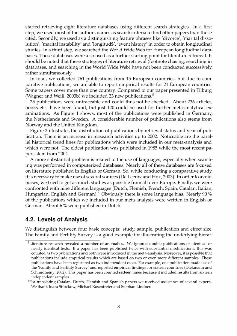
25 publications were untraceable and could thus not be checked. About 236 articles,books etc. have been found, but just 120 could be used for further meta-analytical ex-aminations. As Figure 1 shows, most of the publications were published in Germany,the Netherlands and Sweden. A considerable number of publications also stems fromNorway and the United Kingdom.
Figure 2 illustrates the distribution of publications by retrieval status and year of pub-lication. There is an increase in reasearch activities up to 2002. Noticeable are the paral-lel historical trend lines for publications which were included in our meta-analysis andwhich were not. The eldest publication was published in 1985 while the most recent pa-pers stem from 2004.
A more substantial problem is related to the use of languages, especially when search-ing was performed in computerized databases. Nearly all of these databases are focusedon literature published in English or German. So, while conducting a comparative study,it is necessary to make use of several sources (De Leeuw and Hox, 2003). In order to avoidbiases, we tried to get as much studies as possible from all over Europe. Finally, we wereconfronted with nine different languages (Dutch, Flemish, French, Spain, Catalan, Italian,Hungarian, English and German).6 Obviously there is some language bias. Nearly 90 %of the publications which we included in our meta-analysis were written in English orGerman. About 6 % were published in Dutch.
4.2. Levels of Analysis
We distinguish between four basic concepts: study, sample, publication and effect size.The Family and Fertility Survey is a good example for illustrating the underlying hierar-
5Literature research revealed a number of anomalies. We ignored double publications of identical ornearly identical texts. If a paper has been published twice with substantial modifications, this wascounted as two publications and both were introduced in the meta-analysis. Moreover, it is possible thatpublications include empirical results which are based on two or even more different samples. Thesepublications have been registered as two independent cases. For example, one publication made use ofthe ’Family and Fertility Survey’ and reported empirical findings for sixteen countries (Diekmann andSchmidheiny, 2002). This paper has been counted sixteen times because it included results from sixteenindependent samples.
6For translating Catalan, Dutch, Flemish and Spanish papers we received assistance of several experts.We thank Inara Stürckow, Michael Rosentreter and Stephan Lindner.
8
Fre
quen
cy
Cro
ss n
atio
nal
Aus
tria
Bel
gium
Fin
land
Fra
nce
Ger
man
y
Gre
ece
Hun
gary
Italy
Net
herla
nds
Nor
way
Pol
and
Spa
in
Sw
eden
Sw
itzer
land
Uni
ted
Kin
gdom
10
20
30
40
50
Only bibliographic informationNot suitable for meta−analysisSuitable for meta−analysis
Figure 1: Results of literature retrieval by retrieval status and country
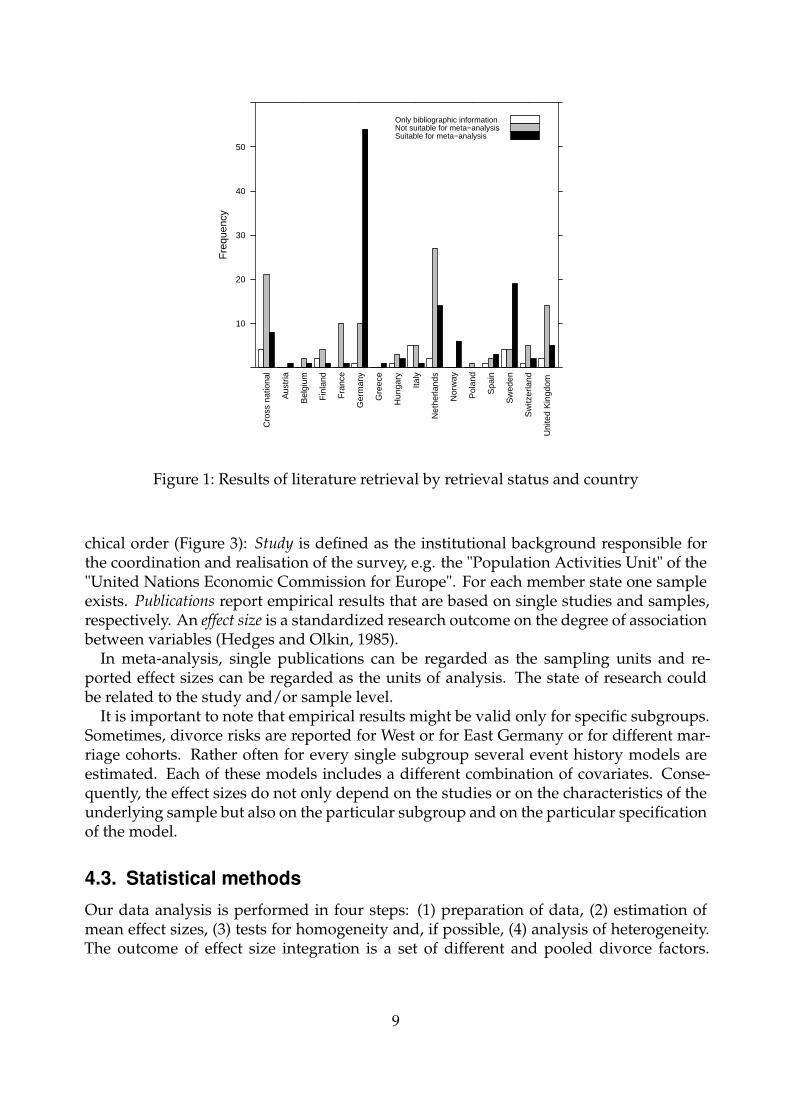
chical order (Figure 3): Study is defined as the institutional background responsible forthe coordination and realisation of the survey, e.g. the "Population Activities Unit" of the"United Nations Economic Commission for Europe". For each member state one sampleexists. Publications report empirical results that are based on single studies and samples,respectively. An effect size is a standardized research outcome on the degree of associationbetween variables (Hedges and Olkin, 1985).
In meta-analysis, single publications can be regarded as the sampling units and re-ported effect sizes can be regarded as the units of analysis. The state of research couldbe related to the study and/or sample level.
It is important to note that empirical results might be valid only for specific subgroups.Sometimes, divorce risks are reported for West or for East Germany or for different mar-riage cohorts. Rather often for every single subgroup several event history models areestimated. Each of these models includes a different combination of covariates. Conse-quently, the effect sizes do not only depend on the studies or on the characteristics of theunderlying sample but also on the particular subgroup and on the particular specificationof the model.
4.3. Statistical methods
Our data analysis is performed in four steps: (1) preparation of data, (2) estimation ofmean effect sizes, (3) tests for homogeneity and, if possible, (4) analysis of heterogeneity.The outcome of effect size integration is a set of different and pooled divorce factors.
9

Year of publication
Fre
quen
cy
1974
1979
1982
1984
1985
1986
1987
1988
1989
1990
1991
1992
1993
1994
1995
1996
1997
1998
1999
2000
2001
2002
2003
2004
0
5
10
15
20
● ● ● ●
● ●
●
●
● ●
● ●
●
●
●
●
●
●
●
●
● ● ●
●
Only bibliographic informationNot suitable for meta−analysisSuitable for meta−analysis
●
Figure 2: Results of literature retrieval by retrieval status and year
Integration will be done by means of calculating weighted mean effect sizes.Many authors describe meta-analytical methods for pooling bivariate statistics (e.g. cor-
relation coefficients, rank order correlations etc., see Bortz and Döring, 1995). In thepresent study we exclusively use regression coefficients7. The pooled effect sizes are at-tained through the computation of the weighted means of all effect sizes. Here, threerequirements are important: (1) It is only meaningful to aggregate effect sizes if at leasttwo single effect sizes exist; (2) effect sizes have to be statistically independent (Fricke andTreinies, 1985; Lipsey and Wilson, 2001); (3) effect sizes are weighted according to theirreliability.
A consequence of the first requirement 1) is that only a small sample of all variables isincluded in meta-analysis. To realize condition 2), it is important to integrate only thoseeffect sizes that are derived from different studies or subsamples. To meet these criteria,effect sizes for similar variables are aggregated for each study. In a second step, meaneffect sizes are pooled across studies (Beelmann and Bliesener, 1994; Bortz and Döring,1995).
To achieve the third requirement 3), we weighted the single effect sizes by their inversevariance (the squared standard error) of each effect size. As suggested by many authors,we use the weighted arithmetic mean (Hedges and Olkin, 1985; Lipsey and Wilson, 2001;Shadish and Haddock, 1994). "Hence, larger weights are assigned to effect sizes from stud-
7Less information exists on synthesizing regression coefficients from multivariate event history models(cf. Greenland, 1987). However, many meta-analysts include such regression coefficients (Amato andKeith, 1991; Karney and Bradbury, 1995; Amato, 2001).
10
Study
Publication A Publication B Publication C
Subgroup A Subgroup B
Model A Model B
Unit of analysis
Sampling unit
Divorce risk A
Divorce risk B
Divorce risk C
Divorce risk D
Effect size A
Effect size B
Effect size C
Effect size D
Effect size A
Effect size B
Effect size D
Figure 3: Levels of analysis
ies with smaller variances and larger withinstudy sample sizes" (Shadish and Haddock,1994). Effect sizes based on a large sample show a higher reliability and will therefore gethigher weights.
4.3.1. Synthesis
The mean effect size ES, weighted by its inverse variance vi, is calculated for n indepen-dent effects sizes ESi as follows:
ES =
∑wi × ESi∑
wi
, (1)
wherewi =
1
vi
=1
SE2. (2)
The inverse variance vi is a weight assigned to the study and equals the inverse squaredstandard error SE.
Another difficulty arises from the aggregation of effect sizes that stem from differentlyspecified models. Coefficients from bivariate or multivariate methods differ according totheir magnitudes and standard errors. Following Lipsey and Wilson (2001), meta-analysismisses adequate procedures of multivariate result integration (e.g. factor analysis or mul-tiple regression). Only very few authors discuss this methodological problem (Amato,2001; Lipsey and Wilson, 2001, 67 ff. and other meta-analyses cited in this book).8
8Some authors simply aggregate effect sizes of coefficients from multivariate models. For example, t-
11
4.3.2. Testing for homogeneity of effect sizes
Two distribution models of effect sizes have to be distinguished. The fixed effects modelassumes all effect sizes to come from one study population. It thus estimates only onepopulation effect size and differences of effect sizes between studies are ignored. The ran-dom effects model assumes the population parameters to be randomly distributed andlocated around a so-called superpopulation. The total variance of effect size estimates re-flects both a study-within-variance and a study-between-variance (Shadish and Haddock,1994): v∗i = σ2 + vi.
In the present case, the pooled effect sizes are expected to be heterogeneous because thedifferent effect sizes are based on different subgroups or model specifications (cf. above).Especially, the integration of partial coefficients is not successfully solved. Coefficientsfrom different models do not estimate the same parameter. Therefore, we particularlymake use of random effects models and expect results of strong heterogeneity.
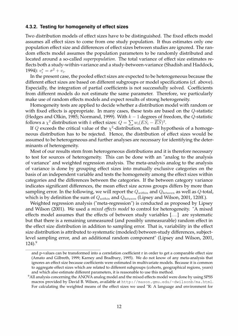
Homogeneity tests are applied to decide whether a distribution model with random orwith fixed effects is appropriate. In many cases, these tests are based on the Q-statistic(Hedges and Olkin, 1985; Normand, 1999). With k − 1 degrees of freedom, the Q-statisticfollows a χ2 distribution with k effect sizes: Q =
∑wi(ESi − ES)2.
If Q exceeds the critical value of the χ2-distribution, the null hypothesis of a homoge-neous distribution has to be rejected. Hence, the distribution of effect sizes would beassumed to be heterogeneous and further analyses are necessary for identifying the deter-minants of heterogeneity.
Most of our results stem from heterogeneous distributions and it is therefore necessaryto test for sources of heterogeneity. This can be done with an "analog to the analysisof variance" and weighted regression analysis. The meta-analysis analog to the analysisof variance is done by grouping effect sizes into mutually exclusive categories on thebasis of an independent variable and tests the homogeneity among the effect sizes withincategories and the differences between the categories. If the between category varianceindicates significant differences, the mean effect size across groups differs by more thansampling error. In the following, we will report the Qwithin and Qbetween as well as Q-total,which is by definition the sum of Qwithin and Qbetween (Lipsey and Wilson, 2001, 120ff.).
Weighted regression analysis ("meta-regression") is conducted as proposed by Lipseyand Wilson (2001). We used a mixed effects model to control for heterogeneity. "A mixedeffects model assumes that the effects of between study variables [. . . ] are systematicbut that there is a remaining unmeasured (and possibly unmeasurable) random effect inthe effect size distribution in addition to sampling error. That is, variability in the effectsize distribution is attributed to systematic (modeled) between-study differences, subject-level sampling error, and an additional random component" (Lipsey and Wilson, 2001,124).9
and p-values can be transformed into a correlation coefficient r in order to get a comparable effect size(Amato and Gilbreth, 1999; Karney and Bradbury, 1995). We do not know of any meta-analysis thatignores an effect size because coefficients were estimated in multivariate models. Because it is commonto aggregate effect sizes which are related to different subgroups (cohorts, geographical regions, years)and which also estimate different parameters, it is reasonable to use this method.
9All analysis concerning the ANOVA analog model and the mixed effects model were done by using SPSSmacros provided by David B. Wilson, available at http://mason.gmu.edu/~dwilsonb/ma.html.For calculating the weighted means of the effect sizes we used "R: A language and environment for
12
4.3.3. Estimation of weights
Serious problems emerge if publications do not report sufficient information to conducta meta-analysis. This is especially true if standard errors of the effect sizes are missing.In our case, less than 20 % of all publications report standard errors or t-values. Theremaining publications only offer information about significance levels using the wellknown ’star symbolism’. To estimate the standard errors the given information should beused at the best possible degree. Details on the estimation procedure of missing standarderrors can be found in Wagner and Weiß (2003a).
5. Results
The aim of this chapter is to describe the variation of effect sizes between and withinEuropean countries. We analyze age at marriage (in years) and premarital cohabitationas indicators of the information level, the birth of children after marriage as indicators ofmarital investments and serveral social resources like the educational attainment of therespondents and of the father’s as well as women’s employment status.
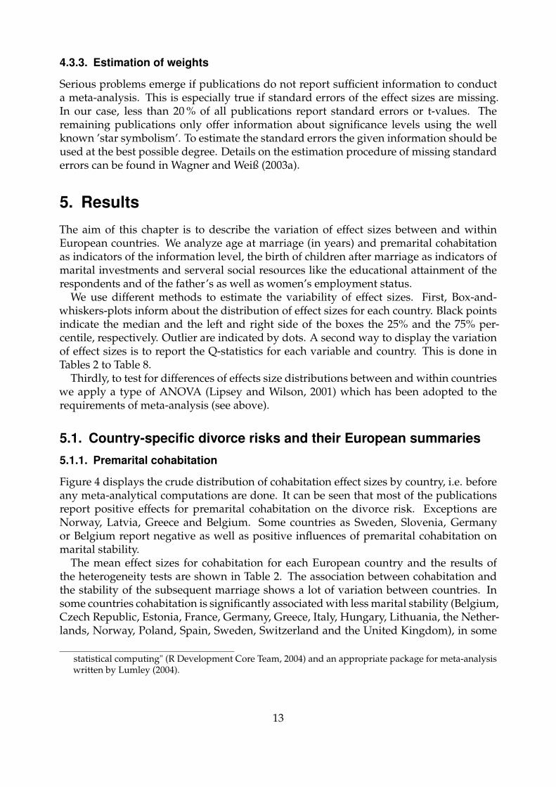
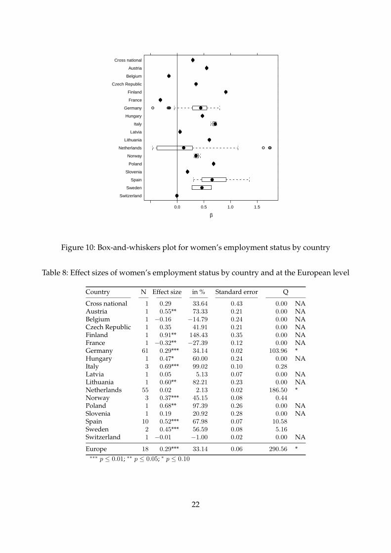
We use different methods to estimate the variability of effect sizes. First, Box-and-whiskers-plots inform about the distribution of effect sizes for each country. Black pointsindicate the median and the left and right side of the boxes the 25% and the 75% per-centile, respectively. Outlier are indicated by dots. A second way to display the variationof effect sizes is to report the Q-statistics for each variable and country. This is done inTables 2 to Table 8.
Thirdly, to test for differences of effects size distributions between and within countrieswe apply a type of ANOVA (Lipsey and Wilson, 2001) which has been adopted to therequirements of meta-analysis (see above).
5.1. Country-specific divorce risks and their European summaries
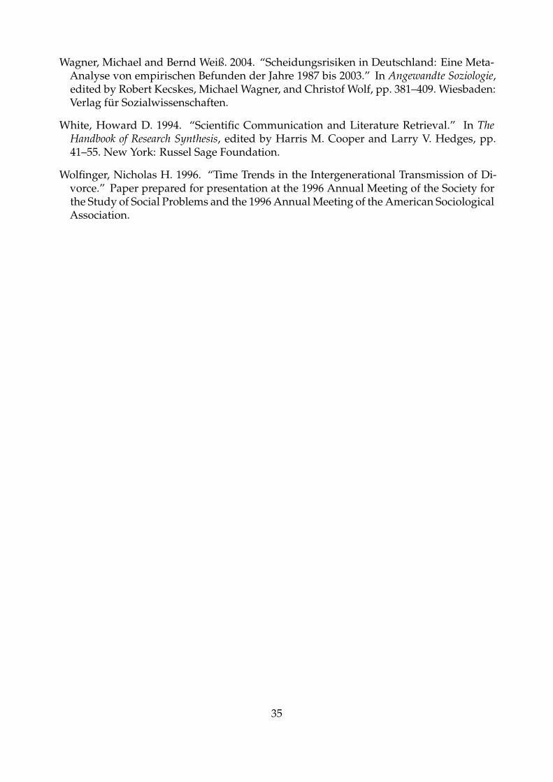
5.1.1. Premarital cohabitation
Figure 4 displays the crude distribution of cohabitation effect sizes by country, i.e. beforeany meta-analytical computations are done. It can be seen that most of the publicationsreport positive effects for premarital cohabitation on the divorce risk. Exceptions areNorway, Latvia, Greece and Belgium. Some countries as Sweden, Slovenia, Germanyor Belgium report negative as well as positive influences of premarital cohabitation onmarital stability.
The mean effect sizes for cohabitation for each European country and the results ofthe heterogeneity tests are shown in Table 2. The association between cohabitation andthe stability of the subsequent marriage shows a lot of variation between countries. Insome countries cohabitation is significantly associated with less marital stability (Belgium,Czech Republic, Estonia, France, Germany, Greece, Italy, Hungary, Lithuania, the Nether-lands, Norway, Poland, Spain, Sweden, Switzerland and the United Kingdom), in some
statistical computing" (R Development Core Team, 2004) and an appropriate package for meta-analysiswritten by Lumley (2004).
13
β
0 1 2
United Kingdom
Switzerland
Sweden
Spain
Slovenia
Poland
Norway
Netherlands
Lithuania
Latvia
Italy
Hungary
Greece
Germany
France
Finland
Estonia
Czech Republic
Belgium
Austria
Cross national ●
●
●
●
●
●●
●
● ●●●● ● ●
●
●●
●
●
●
●●● ●
●●
●
●
●
●
●●
●
Figure 4: Box-and-whiskers plot for premarital cohabitation by country
countries it is not related to marital stability (Austria, Finland, Latvia, Slovenia), and inone country – Greece – it increases marital stability.
Heterogeneity tests reveal considerable variation of the cohabitation effect within coun-tries (Belgium, Germany, the Netherlands, Sweden and United Kingdom). This mightbe due to the fact that the size and the direction of the cohabitation effect differs accord-ing to the specification of the underlying statistical model, especially with respect to theinclusion of control variables.
The European overall effect indicates a positve relationship between cohabitation andthe risk of divorce, i.e. cohabiting couples have a 31% higher risk to divorce than coupleswho do not share a common household before marriage.
A graphical representation of these findings can be found in Figure 13 (appendix). Thistype of plot is called forest plot. Each country-specific effect size and its 95 %-confidenceinterval is plotted. The overall value for Europe can be found at the bottom of the Figure.Each effect size is inverse proportional to its standard error, i.e. "better" estimates areindicated by larger squares.
5.1.2. Age at Marriage
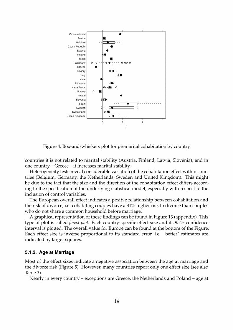
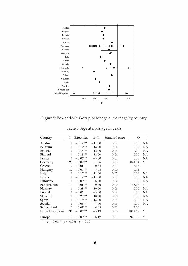
Most of the effect sizes indicate a negative association between the age at marriage andthe divorce risk (Figure 5). However, many countries report only one effect size (see alsoTable 3).
Nearly in every country – exceptions are Greece, the Netherlands and Poland – age at
14
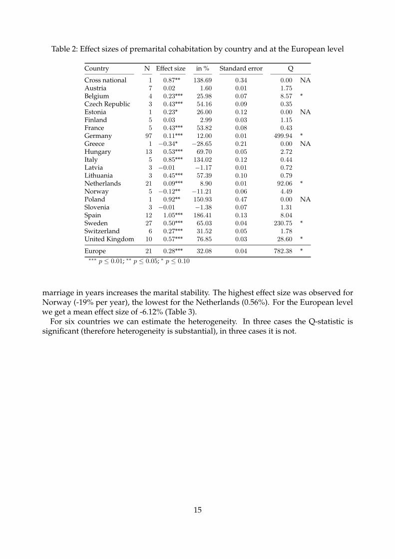
Table 2: Effect sizes of premarital cohabitation by country and at the European level
Country N Effect size in % Standard error Q
Cross national 1 0.87** 138.69 0.34 0.00 NAAustria 7 0.02 1.60 0.01 1.75Belgium 4 0.23*** 25.98 0.07 8.57 *Czech Republic 3 0.43*** 54.16 0.09 0.35Estonia 1 0.23* 26.00 0.12 0.00 NAFinland 5 0.03 2.99 0.03 1.15France 5 0.43*** 53.82 0.08 0.43Germany 97 0.11*** 12.00 0.01 499.94 *Greece 1 −0.34* −28.65 0.21 0.00 NAHungary 13 0.53*** 69.70 0.05 2.72Italy 5 0.85*** 134.02 0.12 0.44Latvia 3 −0.01 −1.17 0.01 0.72Lithuania 3 0.45*** 57.39 0.10 0.79Netherlands 21 0.09*** 8.90 0.01 92.06 *Norway 5 −0.12** −11.21 0.06 4.49Poland 1 0.92** 150.93 0.47 0.00 NASlovenia 3 −0.01 −1.38 0.07 1.31Spain 12 1.05*** 186.41 0.13 8.04Sweden 27 0.50*** 65.03 0.04 230.75 *Switzerland 6 0.27*** 31.52 0.05 1.78United Kingdom 10 0.57*** 76.85 0.03 28.60 *
Europe 21 0.28*** 32.08 0.04 782.38 *∗∗∗ p ≤ 0.01; ∗∗ p ≤ 0.05; ∗ p ≤ 0.10
marriage in years increases the marital stability. The highest effect size was observed forNorway (-19% per year), the lowest for the Netherlands (0.56%). For the European levelwe get a mean effect size of -6.12% (Table 3).
For six countries we can estimate the heterogeneity. In three cases the Q-statistic issignificant (therefore heterogeneity is substantial), in three cases it is not.
15
β
−0.3 −0.2 −0.1 0.0 0.1
United Kingdom
Switzerland
Sweden
Spain
Slovenia
Poland
Norway
Netherlands
Lithuania
Latvia
Italy
Hungary
Greece
Germany
France
Finland
Estonia
Belgium
Austria ●
●
●
●
●
●● ●●●●●● ●● ● ●●
●
●
●
●
●
●●
●
●
●
●
●
●
●● ●●●●
Figure 5: Box-and-whiskers plot for age at marriage by country
Table 3: Age at marriage in years
Country N Effect size in % Standard error Q
Austria 1 −0.12*** −11.00 0.04 0.00 NABelgium 1 −0.14*** −13.00 0.04 0.00 NAEstonia 1 −0.13*** −12.00 0.04 0.00 NAFinland 1 −0.13*** −12.00 0.04 0.00 NAFrance 1 −0.05*** −5.00 0.02 0.00 NAGermany 225 −0.02*** −1.95 0.00 841.84 *Greece 2 −0.01 −0.64 0.01 6.16Hungary 17 −0.06*** −5.58 0.00 6.43Italy 1 −0.15*** −14.00 0.05 0.00 NALatvia 1 −0.12*** −11.00 0.04 0.00 NALithuania 1 −0.06** −6.00 0.02 0.00 NANetherlands 10 0.01*** 0.56 0.00 138.16 *Norway 1 −0.21*** −19.00 0.06 0.00 NAPoland 1 −0.05 −5.00 0.08 0.00 NASlovenia 1 −0.20*** −18.00 0.06 0.00 NASpain 1 −0.16*** −15.00 0.05 0.00 NASweden 1 −0.07** −7.00 0.03 0.00 NASwitzerland 2 −0.07*** −6.42 0.02 2.06United Kingdom 35 −0.05*** −5.19 0.00 1877.58 *
Europe 19 −0.06*** −6.12 0.01 978.99 *∗∗∗ p ≤ 0.01; ∗∗ p ≤ 0.05; ∗ p ≤ 0.10
16
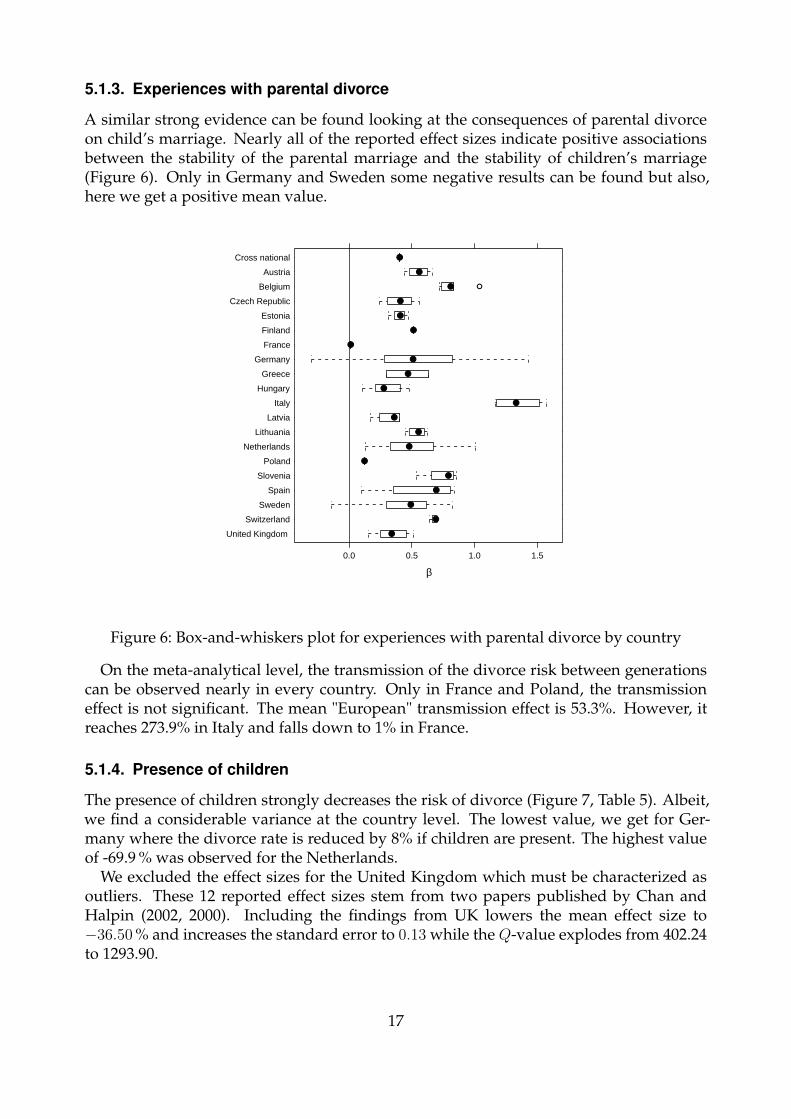
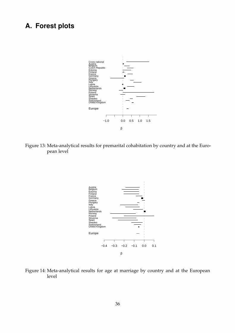
5.1.3. Experiences with parental divorce
A similar strong evidence can be found looking at the consequences of parental divorceon child’s marriage. Nearly all of the reported effect sizes indicate positive associationsbetween the stability of the parental marriage and the stability of children’s marriage(Figure 6). Only in Germany and Sweden some negative results can be found but also,here we get a positive mean value.
β
0.0 0.5 1.0 1.5
United Kingdom
Switzerland
Sweden
Spain
Slovenia
Poland
Netherlands
Lithuania
Latvia
Italy
Hungary
Greece
Germany
France
Finland
Estonia
Czech Republic
Belgium
Austria
Cross national ●
●
● ●
●
●
●
●
●
●
●
●
●
●
●
●
●
●
●
●
●
Figure 6: Box-and-whiskers plot for experiences with parental divorce by country
On the meta-analytical level, the transmission of the divorce risk between generationscan be observed nearly in every country. Only in France and Poland, the transmissioneffect is not significant. The mean "European" transmission effect is 53.3%. However, itreaches 273.9% in Italy and falls down to 1% in France.
5.1.4. Presence of children
The presence of children strongly decreases the risk of divorce (Figure 7, Table 5). Albeit,we find a considerable variance at the country level. The lowest value, we get for Ger-many where the divorce rate is reduced by 8% if children are present. The highest valueof -69.9 % was observed for the Netherlands.
We excluded the effect sizes for the United Kingdom which must be characterized asoutliers. These 12 reported effect sizes stem from two papers published by Chan andHalpin (2002, 2000). Including the findings from UK lowers the mean effect size to−36.50 % and increases the standard error to 0.13 while the Q-value explodes from 402.24to 1293.90.
17
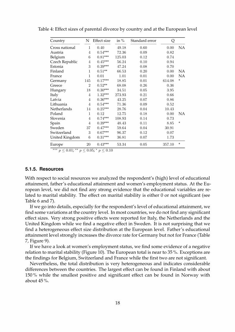
Table 4: Effect sizes of parental divorce by country and at the European level
Country N Effect size in % Standard error Q
Cross national 1 0.40 49.18 0.60 0.00 NAAustria 4 0.54*** 72.36 0.09 0.82Belgium 6 0.81*** 125.03 0.12 0.74Czech Republic 4 0.45*** 56.24 0.10 0.94Estonia 3 0.39*** 47.24 0.08 0.70Finland 1 0.51** 66.53 0.20 0.00 NAFrance 1 0.01 1.01 0.01 0.00 NAGermany 145 0.17*** 18.85 0.01 614.08 *Greece 2 0.52** 68.08 0.26 0.36Hungary 18 0.30*** 34.51 0.05 3.95Italy 4 1.32*** 273.93 0.21 0.66Latvia 4 0.36*** 43.25 0.07 0.86Lithuania 4 0.54*** 71.36 0.09 0.52Netherlands 14 0.25*** 28.76 0.04 10.43Poland 1 0.12 12.75 0.18 0.00 NASlovenia 4 0.74*** 108.93 0.14 0.73Spain 4 0.39*** 48.43 0.11 8.85 *Sweden 37 0.47*** 59.64 0.04 30.91Switzerland 3 0.67*** 96.37 0.12 0.07United Kingdom 6 0.31*** 36.81 0.07 1.73
Europe 20 0.43*** 53.34 0.05 357.10 *∗∗∗ p ≤ 0.01; ∗∗ p ≤ 0.05; ∗ p ≤ 0.10
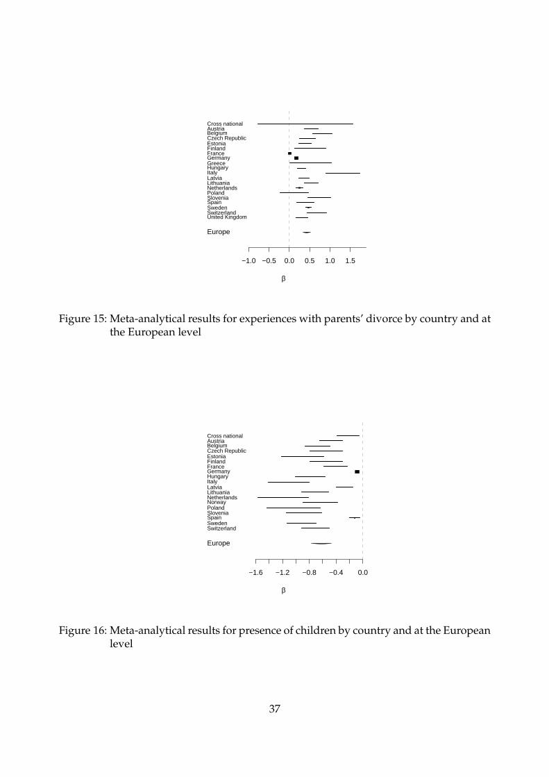
5.1.5. Resources
With respect to social resources we analyzed the respondent’s (high) level of educationalattainment, father’s educational attainment and women’s employment status. At the Eu-ropean level, we did not find any strong evidence that the educational variables are re-lated to marital stability. The effect on marital stability is either 0 or not significant (seeTable 6 and 7).
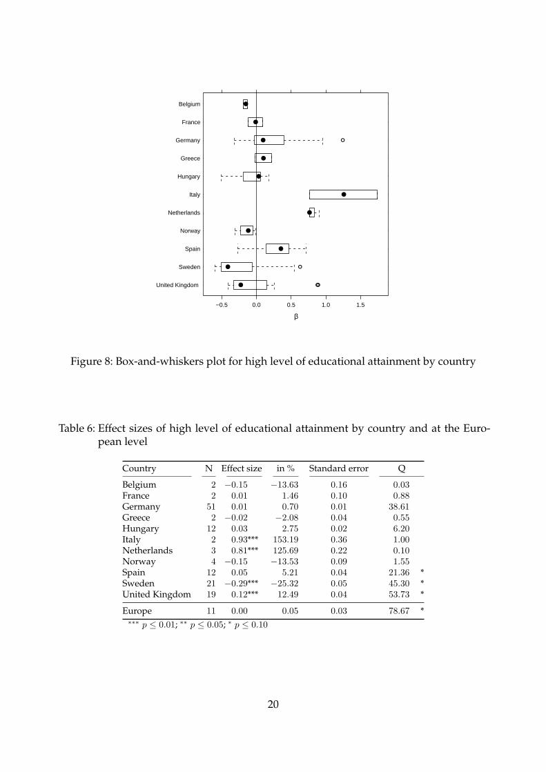
If we go into details, especially for the respondent’s level of educational attainment, wefind some variations at the country level. In most countries, we do not find any significanteffect sizes. Very strong positive effects were reported for Italy, the Netherlands and theUnited Kingdom while we find a negative effect in Sweden. It is not surprising that wefind a heterogeneous effect size distribution at the European level. Father’s educationalattainment level strongly increases the divorce rate for Germany but not for France (Table7, Figure 9).
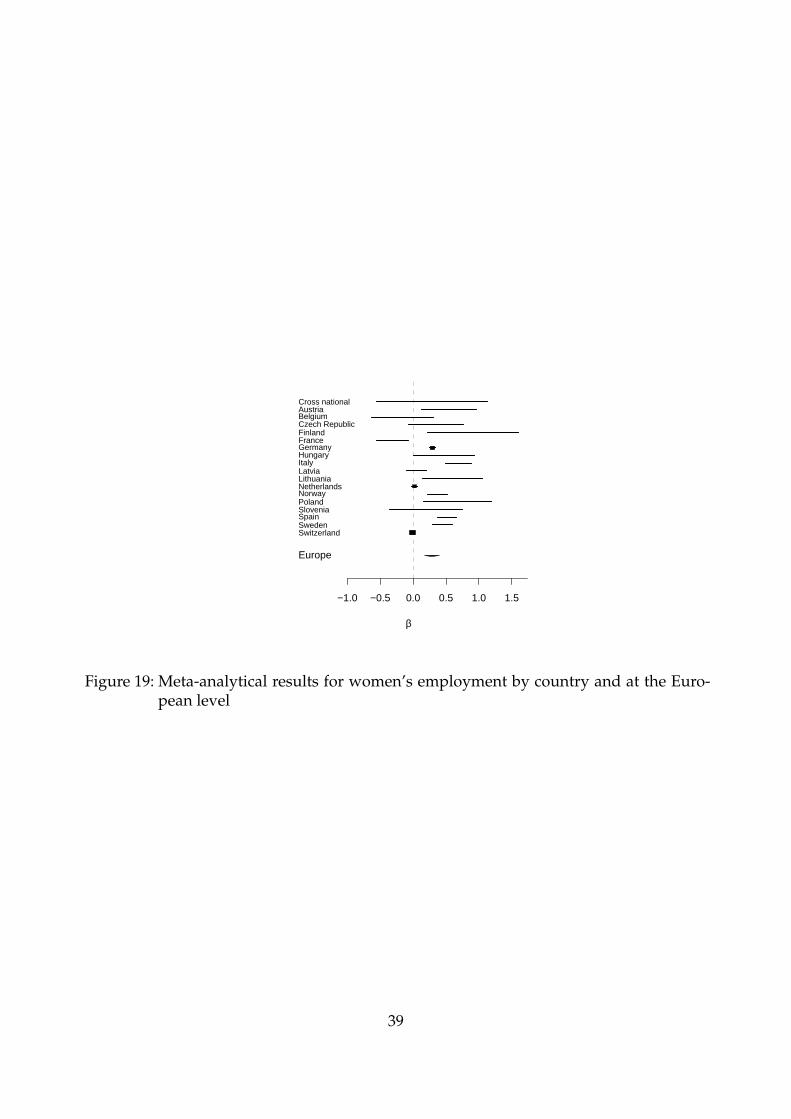
If we have a look at women’s employment status, we find some evidence of a negativerelation to marital stability (Figure 10). The European total is near to 35 %. Exceptions arethe findings for Belgium, Switzerland and France while the first two are not significant.
Nevertheless, the total distribution is very heterogeneous and indicates considerabledifferences between the countries. The largest effect can be found in Finland with about150 % while the smallest positive and significant effect can be found in Norway withabout 45 %.
18

β
−2.5 −2.0 −1.5 −1.0 −0.5 0.0
Switzerland
Sweden
Spain
Slovenia
Poland
Norway
Netherlands
Lithuania
Latvia
Italy
Hungary
Germany
France
Finland
Estonia
Czech Republic
Belgium
Austria
Cross national ●
●
● ●
●
●
●
●
●●●● ● ●●● ●●●
●
●
●
●
●
●
●
●
●
●
●
Figure 7: Box-and-whiskers plot for presence of children by country
Table 5: Effect sizes of presence of children by country and at the European level
Country N Effect size in % Standard error Q
Cross national 1 −0.22** −19.75 0.09 0.00 NAAustria 6 −0.48*** −37.86 0.09 16.38 *Belgium 7 −0.67*** −49.08 0.10 7.40Czech Republic 3 −0.54*** −41.95 0.12 2.90Estonia 4 −0.90*** −59.21 0.16 5.22Finland 4 −0.55*** −42.13 0.12 13.20 *France 6 −0.41*** −33.50 0.09 7.21Germany 91 −0.08*** −8.09 0.01 199.69 *Hungary 6 −0.78*** −54.32 0.11 13.47 *Italy 6 −1.11*** −67.06 0.16 9.45 *Latvia 6 −0.27*** −23.58 0.06 36.64 *Lithuania 6 −0.72*** −51.13 0.10 8.90Netherlands 9 −1.19*** −69.61 0.19 5.62Norway 4 −0.63*** −46.90 0.13 6.03Poland 4 −1.03*** −64.44 0.20 6.60 *Slovenia 6 −0.88*** −58.51 0.14 7.26Spain 10 −0.12*** −11.48 0.04 40.59 *Sweden 11 −0.92*** −60.11 0.11 10.25Switzerland 6 −0.71*** −50.71 0.10 12.59 *
Europe 19 −0.62*** −46.20 0.08 402.24 *∗∗∗ p ≤ 0.01; ∗∗ p ≤ 0.05; ∗ p ≤ 0.10
19
β
−0.5 0.0 0.5 1.0 1.5
United Kingdom
Sweden
Spain
Norway
Netherlands
Italy
Hungary
Greece
Germany
France
Belgium ●
●
● ●
●
●
●
●
●
●
● ●
● ●●
Figure 8: Box-and-whiskers plot for high level of educational attainment by country
Table 6: Effect sizes of high level of educational attainment by country and at the Euro-pean level
Country N Effect size in % Standard error Q
Belgium 2 −0.15 −13.63 0.16 0.03France 2 0.01 1.46 0.10 0.88Germany 51 0.01 0.70 0.01 38.61Greece 2 −0.02 −2.08 0.04 0.55Hungary 12 0.03 2.75 0.02 6.20Italy 2 0.93*** 153.19 0.36 1.00Netherlands 3 0.81*** 125.69 0.22 0.10Norway 4 −0.15 −13.53 0.09 1.55Spain 12 0.05 5.21 0.04 21.36 *Sweden 21 −0.29*** −25.32 0.05 45.30 *United Kingdom 19 0.12*** 12.49 0.04 53.73 *
Europe 11 0.00 0.05 0.03 78.67 *∗∗∗ p ≤ 0.01; ∗∗ p ≤ 0.05; ∗ p ≤ 0.10
20
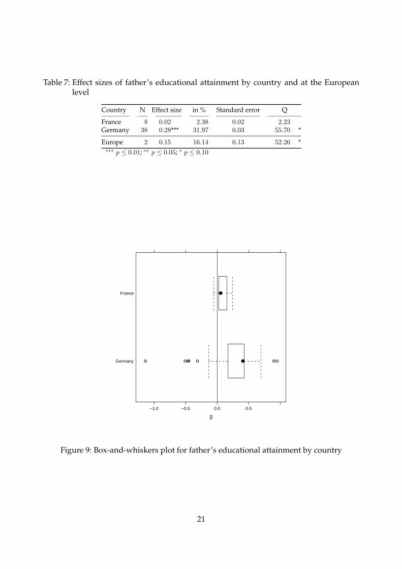
Table 7: Effect sizes of father’s educational attainment by country and at the Europeanlevel
Country N Effect size in % Standard error Q
France 8 0.02 2.38 0.02 2.23Germany 38 0.28*** 31.97 0.03 55.70 *
Europe 2 0.15 16.14 0.13 52.26 *∗∗∗ p ≤ 0.01; ∗∗ p ≤ 0.05; ∗ p ≤ 0.10
β
−1.0 −0.5 0.0 0.5
Germany
France ●
●● ● ●● ● ●●
Figure 9: Box-and-whiskers plot for father’s educational attainment by country
21
β
0.0 0.5 1.0 1.5
Switzerland
Sweden
Spain
Slovenia
Poland
Norway
Netherlands
Lithuania
Latvia
Italy
Hungary
Germany
France
Finland
Czech Republic
Belgium
Austria
Cross national ●
●
●
●
●
●
●●●●● ●
●
●
●
●
● ●● ●
●
●
●
●
●
●
Figure 10: Box-and-whiskers plot for women’s employment status by country
Table 8: Effect sizes of women’s employment status by country and at the European level
Country N Effect size in % Standard error Q
Cross national 1 0.29 33.64 0.43 0.00 NAAustria 1 0.55** 73.33 0.21 0.00 NABelgium 1 −0.16 −14.79 0.24 0.00 NACzech Republic 1 0.35 41.91 0.21 0.00 NAFinland 1 0.91** 148.43 0.35 0.00 NAFrance 1 −0.32** −27.39 0.12 0.00 NAGermany 61 0.29*** 34.14 0.02 103.96 *Hungary 1 0.47* 60.00 0.24 0.00 NAItaly 3 0.69*** 99.02 0.10 0.28Latvia 1 0.05 5.13 0.07 0.00 NALithuania 1 0.60** 82.21 0.23 0.00 NANetherlands 55 0.02 2.13 0.02 186.50 *Norway 3 0.37*** 45.15 0.08 0.44Poland 1 0.68** 97.39 0.26 0.00 NASlovenia 1 0.19 20.92 0.28 0.00 NASpain 10 0.52*** 67.98 0.07 10.58Sweden 2 0.45*** 56.59 0.08 5.16Switzerland 1 −0.01 −1.00 0.02 0.00 NA
Europe 18 0.29*** 33.14 0.06 290.56 *∗∗∗ p ≤ 0.01; ∗∗ p ≤ 0.05; ∗ p ≤ 0.10
22
5.2. Publication characteristics and divorce risks
We found strong evidence that all mean effect sizes at the European level are significantlyheterogeneous. This heterogeneity could be a consequence of societal factors or of differ-ent measurement issues and model specifications.
In the following, we test whether the number of variables per model affects the effectsizes. Table 9 presents the results from a number of bivariate regressions. All analyseswere performed at the level of effect sizes, not countries. For example: the analysis forcohabitation was based on 233 effect sizes.
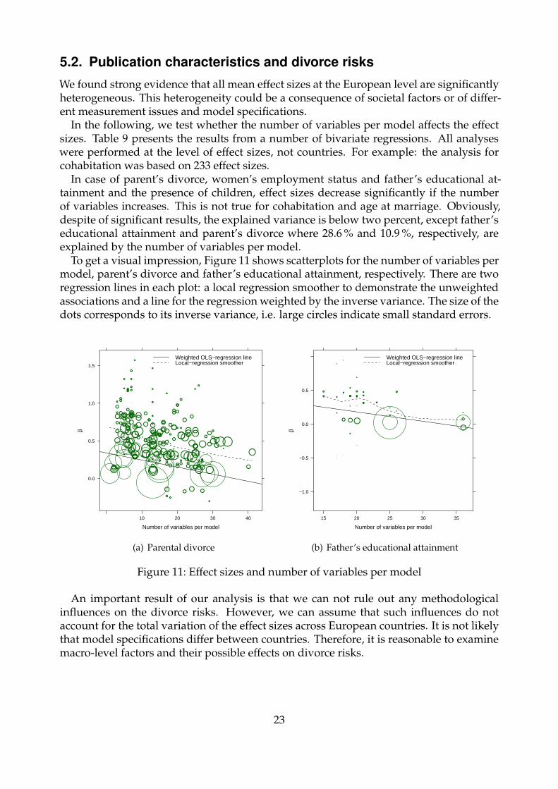
In case of parent’s divorce, women’s employment status and father’s educational at-tainment and the presence of children, effect sizes decrease significantly if the numberof variables increases. This is not true for cohabitation and age at marriage. Obviously,despite of significant results, the explained variance is below two percent, except father’seducational attainment and parent’s divorce where 28.6 % and 10.9 %, respectively, areexplained by the number of variables per model.
To get a visual impression, Figure 11 shows scatterplots for the number of variables permodel, parent’s divorce and father’s educational attainment, respectively. There are tworegression lines in each plot: a local regression smoother to demonstrate the unweightedassociations and a line for the regression weighted by the inverse variance. The size of thedots corresponds to its inverse variance, i.e. large circles indicate small standard errors.
Number of variables per model
β
10 20 30 40
0.0
0.5
1.0
1.5
●●
●●
●
●
●
●
●
●
●
●●
●●
●●●
●
●
●●
●
●
●
●
● ●
●
●
●
●
●
●
●
●
●
●●
●
●
●●
●
●
●
●
●
●
●
●
●
●
●
●
●
●
●
●
●
●
●
●
●
●
●
●
●
●●
●●
●
●
●
●
●
●
●
●
●
●
●
●●
●
● ● ●●●●
●●
●
●●●● ●●●●
●
● ●● ●
●●
●
●
●
●
●● ●
●
●
●
●
●
●
●
●
●
●
●
●●
●
●
●
●
●
●
●
● ●
●
●
●
●
●
●
●●
●
●
●
●
●
●
● ●
● ●
●
●
●●
●
●
●●
●
●
●
●
●
●
●
●
●
●
●●●
● ●●
●
●
● ●● ●
● ●
●
●
●
●
●
●
●●
●
●
●●
●
●
●
●●●● ●
●●
●
● ●
●●●
●●●
●●●
●
● ●
●●
●
●●
●
●●
● ●●
●●
●●●
Weighted OLS−regression lineLocal−regression smoother
(a) Parental divorce
Number of variables per model
β
15 20 25 30 35
−1.0
−0.5
0.0
0.5
●
●
●
●
●
● ●
●●
●
●
●
●●
●
●
●
●
●
●
●
●
●
●
●
●
●
●
●
●
●●
●
●
●
●
●
●
●
●
●
● ●
Weighted OLS−regression lineLocal−regression smoother
(b) Father’s educational attainment
Figure 11: Effect sizes and number of variables per model
An important result of our analysis is that we can not rule out any methodologicalinfluences on the divorce risks. However, we can assume that such influences do notaccount for the total variation of the effect sizes across European countries. It is not likelythat model specifications differ between countries. Therefore, it is reasonable to examinemacro-level factors and their possible effects on divorce risks.
23
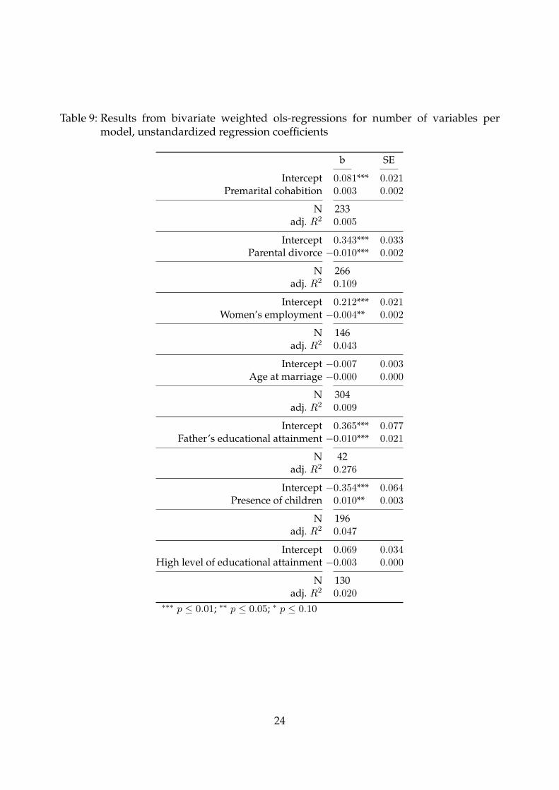
Table 9: Results from bivariate weighted ols-regressions for number of variables permodel, unstandardized regression coefficients
b SE
Intercept 0.081*** 0.021Premarital cohabition 0.003 0.002
N 233adj. R2 0.005
Intercept 0.343*** 0.033Parental divorce −0.010*** 0.002
N 266adj. R2 0.109
Intercept 0.212*** 0.021Women’s employment −0.004** 0.002
N 146adj. R2 0.043
Intercept −0.007 0.003Age at marriage −0.000 0.000
N 304adj. R2 0.009
Intercept 0.365*** 0.077Father’s educational attainment −0.010*** 0.021
N 42adj. R2 0.276
Intercept −0.354*** 0.064Presence of children 0.010** 0.003
N 196adj. R2 0.047
Intercept 0.069 0.034High level of educational attainment −0.003 0.000
N 130adj. R2 0.020
∗∗∗ p ≤ 0.01; ∗∗ p ≤ 0.05; ∗ p ≤ 0.10
24
5.3. Context variables and divorce risks
5.3.1. Macro-level indicators
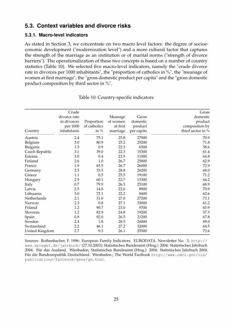
As stated in Section 3, we concentrate on two macro level factors: the degree of socioe-conomic development ("modernization level") and a more cultural factor that capturesthe strength of the marriage as an institution or of marital norms ("strength of divorcebarriers"). The operationalization of these two concepts is based on a number of countrystatistics (Table 10). We selected five macro-level indicators, namely the "crude divorcerate in divorces per 1000 inhabitants", the "proportion of catholics in %", the "meanage ofwomen at first marriage", the "gross domestic product per capita" and the "gross domesticproduct composition by third sector in %".
Table 10: Country-specific indicators
Crude Grossdivorce rate Meanage Gross domesticin divorces Proportion of women domestic product
per 1000 of catholics at first product composition byCountry inhabitants in % marriage per capita third sector in %
Austria 2.4 75.1 25.8 27900 70.9Belgium 3.0 80.9 25.2 29200 71.8Bulgaria 1.3 0.9 22.3 6500 58.6Czech Republic 3.1 39.0 22.3 15300 61.4Estonia 3.0 0.4 23.5 11000 64.8Finland 2.6 1.0 26.7 25800 62.9France 1.9 65.5 26.7 26000 72.9Germany 2.5 33.5 28.8 26200 68.0Greece 1.1 0.5 25.5 19100 71.2Hungary 2.5 60.1 22.7 13300 64.2Italy 0.7 79.9 26.3 25100 68.9Latvia 2.5 14.8 22.6 8900 70.9Lithuania 3.0 72.1 22.2 8400 62.6Netherlands 2.1 31.0 27.0 27200 73.1Norway 2.3 0.8 27.1 33000 61.2Poland 1.2 90.7 23.0 9700 65.9Slovenia 1.2 82.9 24.8 19200 57.3Spain 0.9 92.0 26.5 21200 67.8Sweden 2.4 1.8 28.5 26000 69.0Switzerland 2.2 46.1 27.2 32000 64.5United Kingdom 2.7 9.3 26.1 25500 72.6
Sources: Rothenbacher, F. 1996: European Family Indicators. EURODATA. Newsletter No. 3; http://www.spiegel.de/jahrbuch/ (27.10.2003); Statistisches Bundesamt (Hrsg.) 2004: Statistisches Jahrbuch2004. Für das Ausland. Wiesbaden; Statistisches Bundesamt (Hrsg.) 2004: Statistisches Jahrbuch 2004.Für die Bundesrepublik Deutschland. Wiesbaden.; The World Factbook http://www.odci.gov/cia/publications/factbook/geos/gm.html.
25
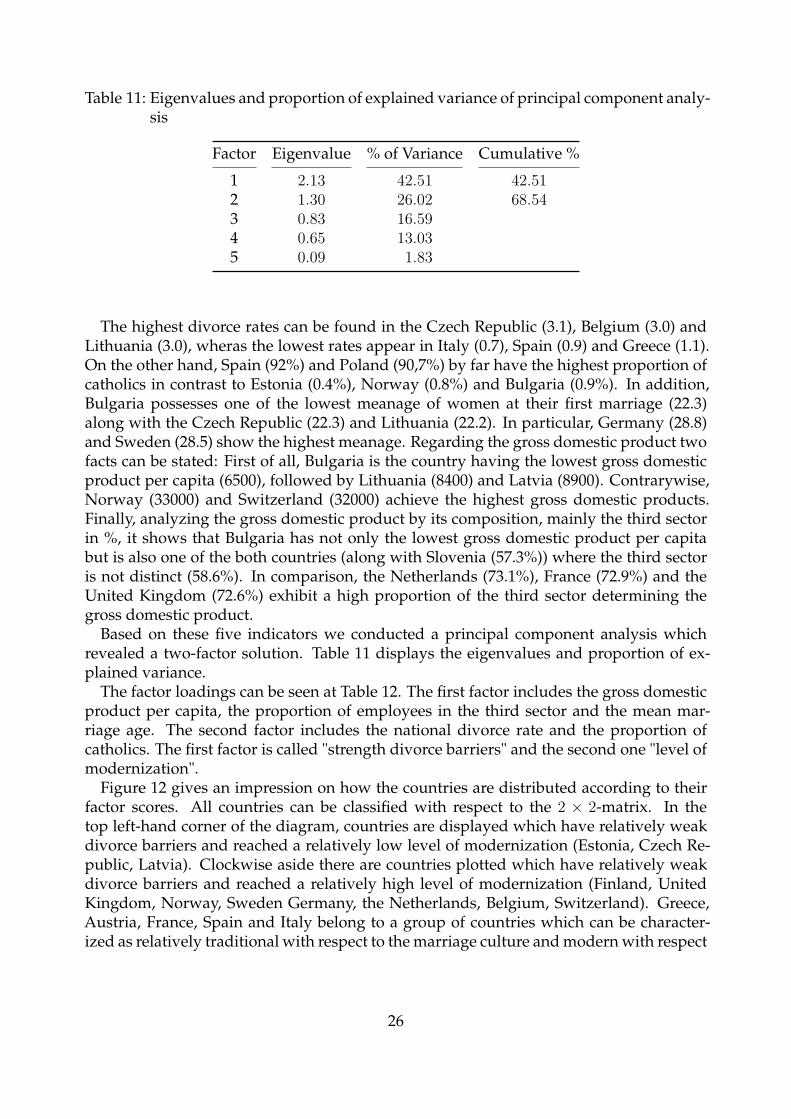
Table 11: Eigenvalues and proportion of explained variance of principal component analy-sis
Factor Eigenvalue % of Variance Cumulative %
1 2.13 42.51 42.512 1.30 26.02 68.543 0.83 16.594 0.65 13.035 0.09 1.83
The highest divorce rates can be found in the Czech Republic (3.1), Belgium (3.0) andLithuania (3.0), wheras the lowest rates appear in Italy (0.7), Spain (0.9) and Greece (1.1).On the other hand, Spain (92%) and Poland (90,7%) by far have the highest proportion ofcatholics in contrast to Estonia (0.4%), Norway (0.8%) and Bulgaria (0.9%). In addition,Bulgaria possesses one of the lowest meanage of women at their first marriage (22.3)along with the Czech Republic (22.3) and Lithuania (22.2). In particular, Germany (28.8)and Sweden (28.5) show the highest meanage. Regarding the gross domestic product twofacts can be stated: First of all, Bulgaria is the country having the lowest gross domesticproduct per capita (6500), followed by Lithuania (8400) and Latvia (8900). Contrarywise,Norway (33000) and Switzerland (32000) achieve the highest gross domestic products.Finally, analyzing the gross domestic product by its composition, mainly the third sectorin %, it shows that Bulgaria has not only the lowest gross domestic product per capitabut is also one of the both countries (along with Slovenia (57.3%)) where the third sectoris not distinct (58.6%). In comparison, the Netherlands (73.1%), France (72.9%) and theUnited Kingdom (72.6%) exhibit a high proportion of the third sector determining thegross domestic product.
Based on these five indicators we conducted a principal component analysis whichrevealed a two-factor solution. Table 11 displays the eigenvalues and proportion of ex-plained variance.
The factor loadings can be seen at Table 12. The first factor includes the gross domesticproduct per capita, the proportion of employees in the third sector and the mean mar-riage age. The second factor includes the national divorce rate and the proportion ofcatholics. The first factor is called "strength divorce barriers" and the second one "level ofmodernization".
Figure 12 gives an impression on how the countries are distributed according to theirfactor scores. All countries can be classified with respect to the 2 × 2-matrix. In thetop left-hand corner of the diagram, countries are displayed which have relatively weakdivorce barriers and reached a relatively low level of modernization (Estonia, Czech Re-public, Latvia). Clockwise aside there are countries plotted which have relatively weakdivorce barriers and reached a relatively high level of modernization (Finland, UnitedKingdom, Norway, Sweden Germany, the Netherlands, Belgium, Switzerland). Greece,Austria, France, Spain and Italy belong to a group of countries which can be character-ized as relatively traditional with respect to the marriage culture and modern with respect
26
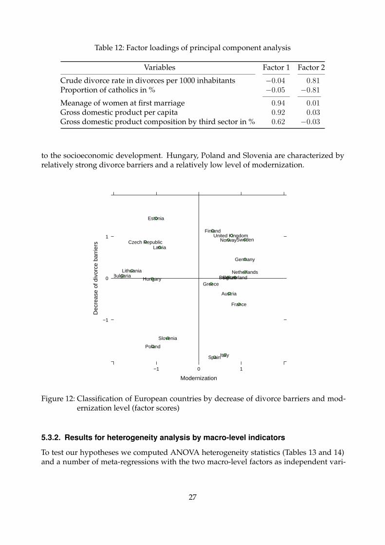
Table 12: Factor loadings of principal component analysis
Variables Factor 1 Factor 2
Crude divorce rate in divorces per 1000 inhabitants −0.04 0.81Proportion of catholics in % −0.05 −0.81
Meanage of women at first marriage 0.94 0.01Gross domestic product per capita 0.92 0.03Gross domestic product composition by third sector in % 0.62 −0.03
to the socioeconomic development. Hungary, Poland and Slovenia are characterized byrelatively strong divorce barriers and a relatively low level of modernization.
Modernization
Dec
reas
e of
div
orce
bar
riers
−1 0 1
−1
0
1
●
●●
●
●
●
●
●
●
●
●
●
● ●
●
●
●
●
●
●
●
Austria
BelgiumBulgaria
Czech Republic
Estonia
Finland
France
Germany
GreeceHungary
Italy
Latvia
Lithuania Netherlands
Norway
Poland
Slovenia
Spain
Sweden
Switzerland
United Kingdom
Figure 12: Classification of European countries by decrease of divorce barriers and mod-ernization level (factor scores)
5.3.2. Results for heterogeneity analysis by macro-level indicators
To test our hypotheses we computed ANOVA heterogeneity statistics (Tables 13 and 14)and a number of meta-regressions with the two macro-level factors as independent vari-
27
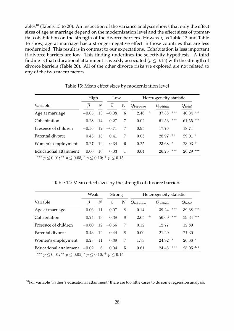
ables10 (Tabels 15 to 20). An inspection of the variance analyses shows that only the effectsizes of age at marriage depend on the modernization level and the effect sizes of premar-ital cohabitation on the strength of the divorce barriers. However, as Table 13 and Table16 show, age at marriage has a stronger negative effect in those countries that are lessmodernized. This result is in contrast to our expectations. Cohabitation is less importantif divorce barriers are low. This finding underlines the selectivity hypothesis. A thirdfinding is that educational attainment is weakly associated (p ≤ 0.15) with the strength ofdivorce barriers (Table 20). All of the other divorce risks we explored are not related toany of the two macro factors.
Table 13: Mean effect sizes by modernization level
High Low Heterogeneity statistic
Variable β N β N Qbetween Qwithin Qtotal
Age at marriage −0.05 13 −0.08 6 2.46 + 37.88 ∗∗∗ 40.34 ∗∗∗
Cohabitation 0.28 14 0.27 7 0.02 61.53 ∗∗∗ 61.55 ∗∗∗
Presence of children −0.56 12 −0.71 7 0.95 17.76 18.71
Parental divorce 0.43 13 0.41 7 0.03 28.97 ∗∗ 29.01 ∗
Women’s employment 0.27 12 0.34 6 0.25 23.68 ∗ 23.93 +
Educational attainment 0.00 10 0.03 1 0.04 26.25 ∗∗∗ 26.29 ***∗∗∗ p ≤ 0.01; ∗∗ p ≤ 0.05; ∗ p ≤ 0.10; + p ≤ 0.15
Table 14: Mean effect sizes by the strength of divorce barriers
Weak Strong Heterogeneity statistic
Variable β N β N Qbetween Qwithin Qtotal
Age at marriage −0.06 11 −0.07 8 0.14 39.24 ∗∗∗ 39.38 ∗∗∗
Cohabitation 0.24 13 0.38 8 2.65 + 56.69 ∗∗∗ 59.34 ∗∗∗
Presence of children −0.60 12 −0.66 7 0.12 12.77 12.89
Parental divorce 0.43 12 0.44 8 0.00 21.29 21.30
Women’s employment 0.23 11 0.39 7 1.73 24.92 ∗ 26.66 ∗
Educational attainment −0.02 6 0.04 5 0.61 24.45 ∗∗∗ 25.05 ***∗∗∗ p ≤ 0.01; ∗∗ p ≤ 0.05; ∗ p ≤ 0.10; + p ≤ 0.15
10For variable "Father’s educational attainment" there are too little cases to do some regression analysis.
28
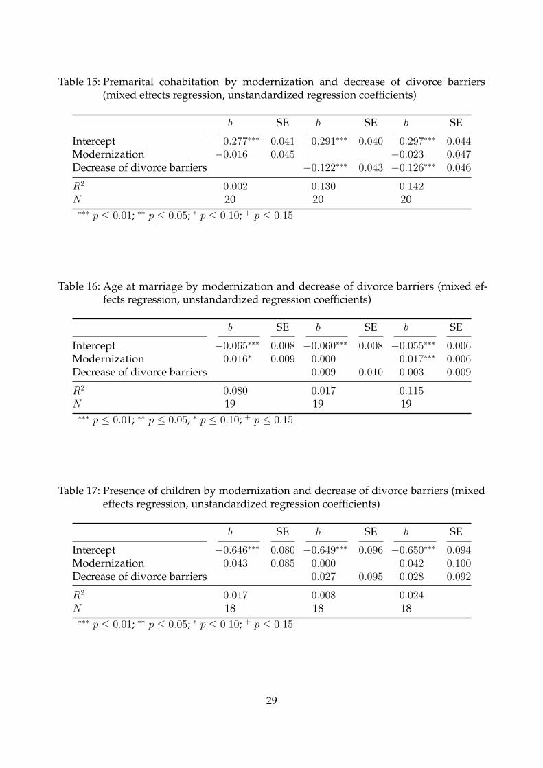
Table 15: Premarital cohabitation by modernization and decrease of divorce barriers(mixed effects regression, unstandardized regression coefficients)
b SE b SE b SE
Intercept 0.277∗∗∗ 0.041 0.291∗∗∗ 0.040 0.297∗∗∗ 0.044Modernization −0.016 0.045 −0.023 0.047Decrease of divorce barriers −0.122∗∗∗ 0.043 −0.126∗∗∗ 0.046
R2 0.002 0.130 0.142N 20 20 20∗∗∗ p ≤ 0.01; ∗∗ p ≤ 0.05; ∗ p ≤ 0.10; + p ≤ 0.15
Table 16: Age at marriage by modernization and decrease of divorce barriers (mixed ef-fects regression, unstandardized regression coefficients)
b SE b SE b SE
Intercept −0.065∗∗∗ 0.008 −0.060∗∗∗ 0.008 −0.055∗∗∗ 0.006Modernization 0.016∗ 0.009 0.000 0.017∗∗∗ 0.006Decrease of divorce barriers 0.009 0.010 0.003 0.009
R2 0.080 0.017 0.115N 19 19 19∗∗∗ p ≤ 0.01; ∗∗ p ≤ 0.05; ∗ p ≤ 0.10; + p ≤ 0.15
Table 17: Presence of children by modernization and decrease of divorce barriers (mixedeffects regression, unstandardized regression coefficients)
b SE b SE b SE
Intercept −0.646∗∗∗ 0.080 −0.649∗∗∗ 0.096 −0.650∗∗∗ 0.094Modernization 0.043 0.085 0.000 0.042 0.100Decrease of divorce barriers 0.027 0.095 0.028 0.092
R2 0.017 0.008 0.024N 18 18 18∗∗∗ p ≤ 0.01; ∗∗ p ≤ 0.05; ∗ p ≤ 0.10; + p ≤ 0.15
29
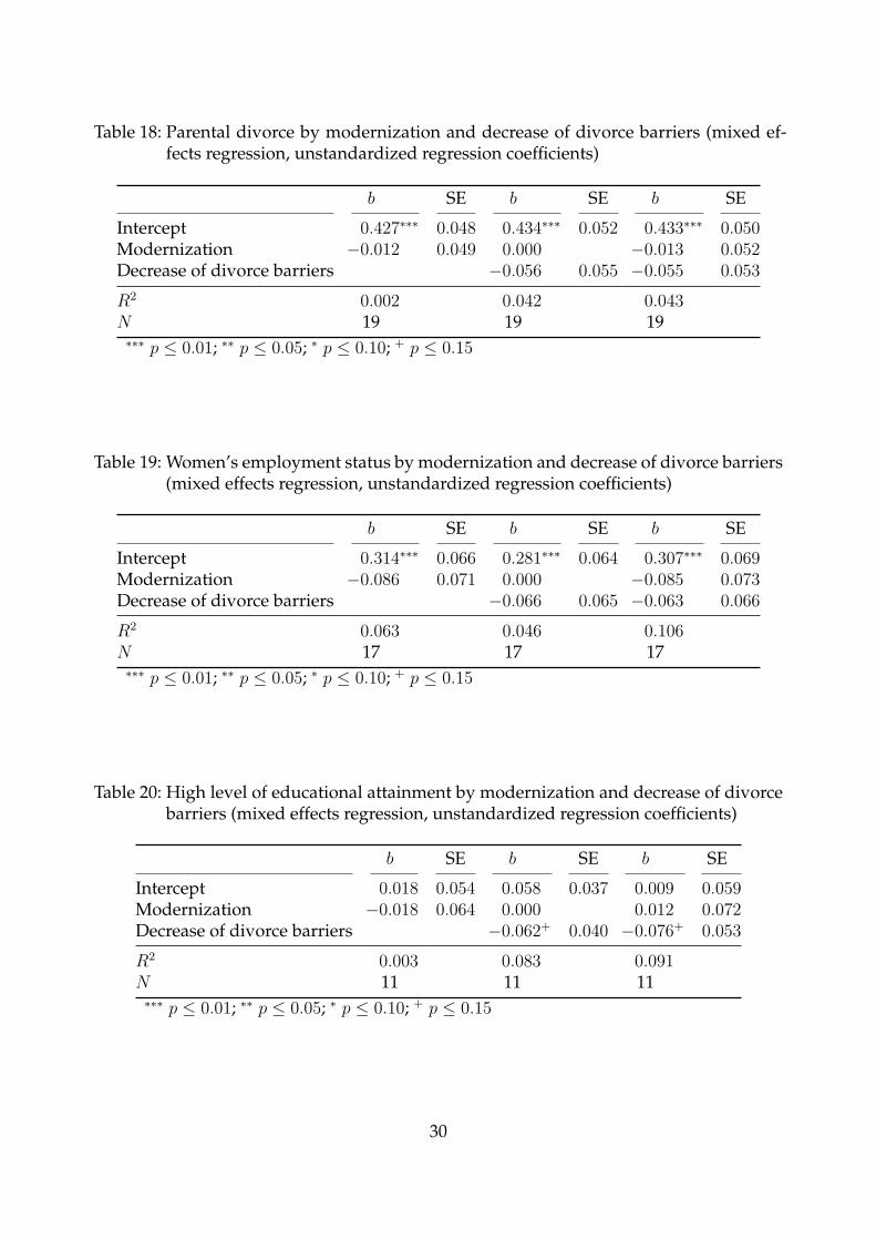
Table 18: Parental divorce by modernization and decrease of divorce barriers (mixed ef-fects regression, unstandardized regression coefficients)
b SE b SE b SE
Intercept 0.427∗∗∗ 0.048 0.434∗∗∗ 0.052 0.433∗∗∗ 0.050Modernization −0.012 0.049 0.000 −0.013 0.052Decrease of divorce barriers −0.056 0.055 −0.055 0.053
R2 0.002 0.042 0.043N 19 19 19∗∗∗ p ≤ 0.01; ∗∗ p ≤ 0.05; ∗ p ≤ 0.10; + p ≤ 0.15
Table 19: Women’s employment status by modernization and decrease of divorce barriers(mixed effects regression, unstandardized regression coefficients)
b SE b SE b SE
Intercept 0.314∗∗∗ 0.066 0.281∗∗∗ 0.064 0.307∗∗∗ 0.069Modernization −0.086 0.071 0.000 −0.085 0.073Decrease of divorce barriers −0.066 0.065 −0.063 0.066
R2 0.063 0.046 0.106N 17 17 17∗∗∗ p ≤ 0.01; ∗∗ p ≤ 0.05; ∗ p ≤ 0.10; + p ≤ 0.15
Table 20: High level of educational attainment by modernization and decrease of divorcebarriers (mixed effects regression, unstandardized regression coefficients)
b SE b SE b SE
Intercept 0.018 0.054 0.058 0.037 0.009 0.059Modernization −0.018 0.064 0.000 0.012 0.072Decrease of divorce barriers −0.062+ 0.040 −0.076+ 0.053
R2 0.003 0.083 0.091N 11 11 11∗∗∗ p ≤ 0.01; ∗∗ p ≤ 0.05; ∗ p ≤ 0.10; + p ≤ 0.15
30
6. Discussion
The aim of this paper was to describe and to explain the heterogeneity of divorce risks inEurope. We concentrated on such divorce risks that play a major role in common divorcemodels: level of information about the partner, marital investments, social resources anddivorce experiences.
European divorce research produced 120 publications that report divorce risks. Thesepublications appeared between the years 1985 and 2004. If one is interested in finding outwhat the results of this research are, there is no alternative to meta-analysis. It is the onlytechnique that allows an exact review of empirical research.
In a first step, we estimated the strength of divorce risks for 21 European countries.On the one hand, we found that rather often estimates of divorce risks vary significantlywithin countries. This is per se an important finding as it shows that we cannot be sureabout the strength of the relationships between the variables even at the national level.In that case, one has to be cautious when calculating a mean effect size as they do notrepresent the distribution of effect sizes adequately. On the other hand, for quite a num-ber of countries divorce risks do not a show strong internal variation. For example, thetransmission effects or the effects for educational attainment do not vary a lot within thecountries. Here, we get rather precise national estimates for certain divorce risks.
A central aim of this study was to explain the variation of the national divorce risksacross Europe. We developed two types of hypotheses. First, we asked whether themodernization level affects divorce risks. As a second macro factor we introduced theprevalence of traditional marriage norms.
Despite of a small sample size, two macro-micro relations were empirically confirmed.Both concern the level of information about the partner before marriage. But – not as ithas been hypothesized – the age effect is not stronger in highly modernized countries butin less modernized countries. The higher the level of modernization the weaker age atmarriage affects marital stability. In highly modernized European countries individualsmarry late and an early marriage is often not compatible with the requirements of theeducational system and the labor market. Early marriages are burdened and are likely tobreak up. But irrespective of this consideration in Eastern Europe – where the moderniza-tion level is relatively low – age at marriage is even more important for an explanation ofmarital stability.
A second hypothesis that has been confirmed is about the association of cohabitationon the divorce rate. In countries where traditional marriage norms are strongly institu-tionalized, cohabitation has a stronger effect than in countries where marriage norms areweaker. This result underlines the selectivity hypothesis.
A third hypothesis that was "nearly" confirmed is related to the role of social resources:the weaker divorce norms are the less important social resources are for an explanationof divorce. The reason should be that social resources are needed to overcome the costs ofa divorce. The higher these costs are the more social resources are required to overcomethese costs.
No empirical support was found with respect to our hypothesis that the associationbetween marital investments and marital stability depends on the modernization levelor the strength of divorce norms. It might be that a country indicator that captures thefamily policy and the infrastructure of child custody is a better explanatory variable. For
31

example, Gerhards/Hölscher 2003 differentiate between three models of family policy"family support", market oriented" and "dual earner". Especially, the implementation ofthe "dual career" model like in Sweden or in East European countries should facilitate adivorce in case of the presence of children. However, one has to take into account thatselectivity processes might counteract such a macro-micro link. In some countries, theformation of a family is more dependent on a stable marriage than in other countries.
How should comparative divorce research be performed? We still believe that meta-analytical techniques are the best procedure to get good estimators of effect sizes at thenational level. An effect size that is based on many studies is better than a effect size thatis only based on a single study. We demonstrated that effect sizes can differ accordingto the model specification. This was especially pronounced with respect to the transmis-sion effect and father’s educational level but surprisingly not for the cohabitation effect.Nevertheless, it is not very likely that these methodological issues account for the varia-tion of divorce risks across countries as the consequences of different model specificationsshould level off when comparing mean divorce risks.
Nevertheless, this study showed that it is difficult to explain the pattern of divorcerisks across Europe. Most of our hypotheses did not find any empirical support. Wedo not have a strong theory and empirical results demonstrate that such factors as themodernization level or the degree at which traditional marriage norms are established ina country are poor predictors of how divorce risks are distributed across Europe.
References
Amato, Paul R. 2001. “Children of Divorce in the 1990s: An Update of the Amato andKeith (1991) Meta-Analysis.” Journal of Family Psychology 15:355–370.
Amato, Paul R. and Joan G. Gilbreth. 1999. “Nonresident Father’s and Children’s Well-Being: A Meta-Analysis.” Journal of Marriage and the Family 61:557–573.
Amato, Paul R. and Bruce Keith. 1991. “Parental Divorce and the Well-Being of Children:A Meta-Analysis.” Psychological Bulletin 110:26–46.
Beelmann, A. and T. Bliesener. 1994. “Aktuelle Probleme und Strategien der Metaanalyse.”Psychologische Rundschau 45:211–233.
Blossfeld, Hans-Peter, Alessandra De Rose, Jan M. Hoem, and Götz Rohwer. 1995. “Edu-cation, Modernization, and the Risk of Marriage Disruption in Sweden, West Germany,and Italy.” In Gender and Family Change in Industrialized Countries, edited by Karen Op-penheim Mason and An-Magritt Jensen, pp. 200–222. Oxford: Clarendon Press.
Blossfeld, Hans-Peter and Rolf Müller. 2002. “Union Disruption in Comparative perspec-tive: The Role of Assortative Partner Choice and Careers of Couples.” InternationalJournal of Sociology 32:3–35.
Bortz, Jürgen and Nicola Döring. 1995. Forschungsmethoden und Evaluation für Sozialwis-senschaftler. Berlin/Heidelberg: Springer-Verlag.
32
Brüderl, Josef and Andreas Diekmann. 1997. “Education and Marriage. A ComparativeStudy.” Manuscript.
Chan, Tak Wing and Brendan Halpin. 2000. “Union Dissolution in the UK.”http://citeseer.ist.psu.edu/492462.html.
Chan, Tak Wing and Brendan Halpin. 2002. “Children and Marital Instability in the UK.”http://citeseer.ist.psu.edu/498477.html.
Cooper, Harris M. 1982. “Scientific guidelines for conducting integrative research re-views.” Review of Educational Research 52:291–302.
De Leeuw, Edith and Joop J. Hox. 2003. “The Use of Meta-Analysis in CrossnationalStudies.” In Cross-Cultural Survey Methods, edited by Janet A. Harkness, Fons van deVijver, and Peter Ph. Mohler, pp. 329–399. Hoboken: John Wiley & Sons.
Diekmann, Andreas and Kurt Schmidheiny. 2002. “The Intergenerational Transmissionof Divorce. Results From a Sixteen-Country Study with the Fertility and Family Sur-vey.” The Second Conference of the European Research Network on Divorce, TilburgUniversity, Netherlands, November 13-14, 2003.
Dourleijn, Edith and Aart C. Liefbroer. 2003. “Unmarried cohabitation and union stability:Testing the role of diffusion using data from 16 European countries.” Manuscript.
Fricke, Reiner and Gerhard Treinies. 1985. Einführung in die Metaanalyse. Bern: Huber.
Gerhards, Jürgen and Michael Hölscher. 2003. “Kulturelle Unterschiede zwischenMitglieds- und Beitrittsländern der EU. Das Beispiel Familien- und Gleichberechti-gungsvorstellungen.” Zeitschrift für Soziologie 32:206–225.
Greenland, Sander. 1987. “Quantitative Methods in the Review of Epidemiologic Litera-ture.” Epidemiologic Reviews 9:1–30.
Hedges, Larry V. and Ingram Olkin. 1985. Statistical Methods for Meta-Analysis. Orlando:Academic Press.
Hill, Paul Bernhard and Johannes Kopp. 1995. Familiensoziologie. Grundlagen und theore-tische Perspektiven. Stuttgart: Teubner.
Karney, Benjamin R. and Thomas N. Bradbury. 1995. “The Longitudinal Course of MaritalQuality and Stability: A Review of Theory, Method and Research.” Psychological Bulletin118:3–34.
Künzler, Jan, Hans-Joachim Schulze, and Suus M.J. van Hekken. 1999. “Welfare States andNormative Orientations Towards Women’s Employment.” Comparative Social Research18:197–225.
Levinger, George. 1965. “Marital Cohesiveness and Dissolution: An Integrative Review.”Journal of Marriage and the Family 27:19–28.
33
Levinger, George. 1982. “A Social Exchange View on the Dissolution of Pair Relation-ships.” In Family Relationships. Rewards and Costs, edited by F. Ivan Nye, pp. 97–121.Beverly Hills: Sage.
Lewis, Robert A. and Graham B. Spanier. 1979. “Theorizing about the Quality and Stabil-ity of Marriage.” In Contemporary Theories About the Family. General Theories/TheoreticalOrientations, edited by Wesley R. Burr, Reuben Hill, F. Ivan Nye, and Ira L. Reiss, vol-ume I, pp. 268–294. New York: Free Press.
Lipsey, Mark W. and David B. Wilson. 2001. Practical Meta-Analysis. Thousand Oaks,California: Sage Publications.
Lumley, Thomas. 2004. rmeta: Meta-analysis. R package version 2.12.
Normand, Sharon-Lise T. 1999. “Tutorial in Biostatistics. Meta-Analysis: Formulating,Evaluating, Combining, and Reporting.” Statistics in Medicine 18:321–359.
R Development Core Team. 2004. R: A language and environment for statistical computing. RFoundation for Statistical Computing, Vienna, Austria. ISBN 3-900051-07-0.
Sabatelli, Ronald M. and Constance L. Shehan. 1993. “Exchange and Resource Theories.”In Sourcebook of Family Theories and Methods. A Contextual Approach, edited by Pauline G.Boss, William J. Doherty, Ralph LaRossa, Walter R. Schumm, and Suzanne K. Steinmetz,pp. 385–417. New York: Plenum Press.
Shadish, William R. and Keith C. Haddock. 1994. “Combining Estimates of Effect Size.”In The Handbook of Research Synthesis, edited by Harris M. Cooper and Larry V. Hedges,pp. 261–281. New York: Russel Sage Foundation.
Trent, Katherine and Scott J. South. 1989. “Structural Determinants of the Divorce Rate:A Cross-societal Analysis.” Journal of Marriage and the Family 51:391–404.
Uunk, Wilfred and Matthijs Kalmijn. 2002. “Welfare State Regimes and the EconomicConsequences of Separation: Evidence from the European Household Panel Survey,1994–1998.” Paper prepared for "The First Conference of the European Research Net-work on Divorce", Florence, Italy, November 14–15, 2002.
Wagner, Michael. 1997. Scheidung in Ost- und Westdeutschland: Zum Verhältnis von Ehesta-bilität und Sozialstruktur. Frankfurt/Main: Campus.
Wagner, Michael and Bernd Weiß. 2002. “A Meta-Analysis of German Research on Di-vorce Risks.” Paper prepared for "The First Conference of the European Research Net-work on Divorce", Florence, Italy, November 14–15, 2002.
Wagner, Michael and Bernd Weiß. 2003a. “Bilanz der deutschen Scheidungsforschung.Versuch einer Meta-Analyse.” Zeitschrift für Soziologie 32:29–49.
Wagner, Michael and Bernd Weiß. 2003b. “Divorce Risks in Europe: An Overview.” Paperprepared for "The Second Conference of the European Research Network on Divorce",Tilburg University, Netherlands, November 13-14, 2003.
34
Wagner, Michael and Bernd Weiß. 2004. “Scheidungsrisiken in Deutschland: Eine Meta-Analyse von empirischen Befunden der Jahre 1987 bis 2003.” In Angewandte Soziologie,edited by Robert Kecskes, Michael Wagner, and Christof Wolf, pp. 381–409. Wiesbaden:Verlag für Sozialwissenschaften.
White, Howard D. 1994. “Scientific Communication and Literature Retrieval.” In TheHandbook of Research Synthesis, edited by Harris M. Cooper and Larry V. Hedges, pp.41–55. New York: Russel Sage Foundation.
Wolfinger, Nicholas H. 1996. “Time Trends in the Intergenerational Transmission of Di-vorce.” Paper prepared for presentation at the 1996 Annual Meeting of the Society forthe Study of Social Problems and the 1996 Annual Meeting of the American SociologicalAssociation.
35
A. Forest plots
β
−1.0 0.0 0.5 1.0 1.5
Cross nationalAustriaBelgiumCzech RepublicEstoniaFinlandFranceGermanyGreeceHungaryItalyLatviaLithuaniaNetherlandsNorwayPolandSloveniaSpainSwedenSwitzerlandUnited Kingdom
Europe
Figure 13: Meta-analytical results for premarital cohabitation by country and at the Euro-pean level
β
−0.4 −0.3 −0.2 −0.1 0.0 0.1
AustriaBelgiumEstoniaFinlandFranceGermanyGreeceHungaryItalyLatviaLithuaniaNetherlandsNorwayPolandSloveniaSpainSwedenSwitzerlandUnited Kingdom
Europe
Figure 14: Meta-analytical results for age at marriage by country and at the Europeanlevel
36
β
−1.0 −0.5 0.0 0.5 1.0 1.5
Cross nationalAustriaBelgiumCzech RepublicEstoniaFinlandFranceGermanyGreeceHungaryItalyLatviaLithuaniaNetherlandsPolandSloveniaSpainSwedenSwitzerlandUnited Kingdom
Europe
Figure 15: Meta-analytical results for experiences with parents’ divorce by country and atthe European level
β
−1.6 −1.2 −0.8 −0.4 0.0
Cross nationalAustriaBelgiumCzech RepublicEstoniaFinlandFranceGermanyHungaryItalyLatviaLithuaniaNetherlandsNorwayPolandSloveniaSpainSwedenSwitzerland
Europe
Figure 16: Meta-analytical results for presence of children by country and at the Europeanlevel
37
β
−0.5 0.0 0.5 1.0 1.5
Belgium
FranceGermany
GreeceHungaryItaly
NetherlandsNorwaySpain
SwedenUnited Kingdom
Europe
Figure 17: Meta-analytical results for high level of educational attainment by country andat the European level
β
−1.0 −0.6 −0.2 0.2
France
Germany
Europe
Figure 18: Meta-analytical results for father’s educational attainment by country and atthe European level
38
β
−1.0 −0.5 0.0 0.5 1.0 1.5
Cross nationalAustriaBelgiumCzech RepublicFinlandFranceGermanyHungaryItalyLatviaLithuaniaNetherlandsNorwayPolandSloveniaSpainSwedenSwitzerland
Europe
Figure 19: Meta-analytical results for women’s employment by country and at the Euro-pean level
39