Embed Size (px)
Citation preview

On the visualization of time-varying complexelectromagnetic field lines in 3D and 4D
fashions
vorgelegt vonDipl.-Inf.
Ibrahim Abu El-Khair
von der Fakultat IV-Elektrotechnik und Informatikder Technischen Universitat Berlin
Zur Erlangung des akademischen Grades
Doktor der Ingenieurwissenschaft-Dr.-Ing.-
genehmigte Dissertation
Promotionsausschuss:
Vorsitzender: Prof. Dr. B. Lutterbeck1. Berichter: Prof. Dr. G. Monich2. Berichter: Prof. Dr. G. Barwolff
Tag der wissenschaftlichen Aussprache: 24. November 2006
Berlin 2006D83

i
Contents
The objectiveness of this thesis xvii
Dedication xvii
Acknowledgment 1
1 Principles of EM Radiation 1
1.1 A single Wire . . . . . . . . . . . . . . . . . . . . . . . . . . . . . . . . . . . . . . . . . 2
1.2 Principle of field detachment shown by small loop and finite length antennas . . . . 4
1.2.1 Derivation of Time-varying Fields for a Hertzian Dipole . . . . . . . . . . . . 7
2 Maxwell’s Equations 15
2.1 The classes of Maxwell’s equations . . . . . . . . . . . . . . . . . . . . . . . . . . . . . 16
2.1.1 Maxwell’s Equations in differential form . . . . . . . . . . . . . . . . . . . . . 18
2.1.2 Maxwell’s equations in integral form . . . . . . . . . . . . . . . . . . . . . . . 19
2.1.3 Maxwell’s equations in transform domain . . . . . . . . . . . . . . . . . . . . 20
2.1.4 Introductory to the phasor-notation . . . . . . . . . . . . . . . . . . . . . . . . 22
2.1.5 Duality . . . . . . . . . . . . . . . . . . . . . . . . . . . . . . . . . . . . . . . . . 28

ii Contents
3 Tracing of Fieldlines 29
3.1 The longitudinal sectors’ approach . . . . . . . . . . . . . . . . . . . . . . . . . . . . . 29
3.2 A synoptical glance on classical methods of field lines representation: . . . . . . . . . 32
3.2.1 A line as the intersection of two surfaces . . . . . . . . . . . . . . . . . . . . . 32
Line density versus flux intensity . . . . . . . . . . . . . . . . . . . . . . . . . . 33
4 E-wall , H-wall and Image theory 35
4.1 Magnetic and electric walls . . . . . . . . . . . . . . . . . . . . . . . . . . . . . . . . . 35
4.2 Image Theory . . . . . . . . . . . . . . . . . . . . . . . . . . . . . . . . . . . . . . . . . 38
5 From EM Fields to fieldlines 43
6 Start points for line tracing 49
6.1 Topology of surface and displacement currents . . . . . . . . . . . . . . . . . . . . . . 49
6.1.1 Discretization of the conducting plane . . . . . . . . . . . . . . . . . . . . . . . 50
6.1.2 Line families . . . . . . . . . . . . . . . . . . . . . . . . . . . . . . . . . . . . . . 53
6.1.3 Chronological visualization of the field evolution . . . . . . . . . . . . . . . . 53
6.1.4 The new surface definitions, applied to a straight wire . . . . . . . . . . . . . 54
7 On the arbitrarily oriented radiators 57
7.1 A provoked solution: Replacement Rules . . . . . . . . . . . . . . . . . . . . . . . . . 58
How does it really work? . . . . . . . . . . . . . . . . . . . . . . . . . . . . . . 58
7.1.1 Limitations . . . . . . . . . . . . . . . . . . . . . . . . . . . . . . . . . . . . . . 59
7.2 Rotation Matrices . . . . . . . . . . . . . . . . . . . . . . . . . . . . . . . . . . . . . . . 60

Contents iii
7.2.1 The Adopted Rotation Matrix . . . . . . . . . . . . . . . . . . . . . . . . . . . . 60
7.2.2 What are transpose Matrices really good for? . . . . . . . . . . . . . . . . . . . 63
A correction . . . . . . . . . . . . . . . . . . . . . . . . . . . . . . . . . . . . . . 64
7.3 To Formulas . . . . . . . . . . . . . . . . . . . . . . . . . . . . . . . . . . . . . . . . . . 65
An example . . . . . . . . . . . . . . . . . . . . . . . . . . . . . . . . . . . . . . 67
Yet another example . . . . . . . . . . . . . . . . . . . . . . . . . . . . . . . . . 67
7.3.1 For an arbitrarily oriented Hertzian Dipole . . . . . . . . . . . . . . . . . . . . 69
magnetic fields . . . . . . . . . . . . . . . . . . . . . . . . . . . . . . . . . . . . 69
Electric Fields . . . . . . . . . . . . . . . . . . . . . . . . . . . . . . . . . . . . . 69
7.3.2 For an arbitrarily oriented finite length linear dipole . . . . . . . . . . . . . . . 70
Magnetic Fields . . . . . . . . . . . . . . . . . . . . . . . . . . . . . . . . . . . . 70
Electric Fields . . . . . . . . . . . . . . . . . . . . . . . . . . . . . . . . . . . . . 70
8 Numerical Approach 73
A minimal requirement . . . . . . . . . . . . . . . . . . . . . . . . . . . . . . . 74
A well-posed Problem . . . . . . . . . . . . . . . . . . . . . . . . . . . . . . . . 74
Sources of error . . . . . . . . . . . . . . . . . . . . . . . . . . . . . . . . . . . . 75
8.0.3 Order of Accuracy, Convergence and Stability of numerical Methods . . . . . 76
8.1 Why to undertake a numerical approach? . . . . . . . . . . . . . . . . . . . . . . . . . 78
8.1.1 The main reason: Discretization . . . . . . . . . . . . . . . . . . . . . . . . . . 78
8.1.2 Which strategies are used to plot the field lines? . . . . . . . . . . . . . . . . . 79
8.2 A system of differential equations . . . . . . . . . . . . . . . . . . . . . . . . . . . . . . 84
8.2.1 Application: Kepler’s Problem; a test problem . . . . . . . . . . . . . . . . . . 86

iv Contents
Kepler’s Laws first . . . . . . . . . . . . . . . . . . . . . . . . . . . . . . . . . . 87
Formulation . . . . . . . . . . . . . . . . . . . . . . . . . . . . . . . . . . . . . . 89
Performance . . . . . . . . . . . . . . . . . . . . . . . . . . . . . . . . . . . . . . 91
9 Results 107
9.1 An omnidirectional radiation . . . . . . . . . . . . . . . . . . . . . . . . . . . . . . . . 107
9.2 A directional radiation . . . . . . . . . . . . . . . . . . . . . . . . . . . . . . . . . . . . 110
9.2.1 A passage to 4D visualization . . . . . . . . . . . . . . . . . . . . . . . . . . . . 112
Appendix 115
A On small square loop Antenna . . . . . . . . . . . . . . . . . . . . . . . . . . . . . . . 115
B On small circular loop Antenna . . . . . . . . . . . . . . . . . . . . . . . . . . . . . . . 123
B.1 The Magnetic Fields . . . . . . . . . . . . . . . . . . . . . . . . . . . . . . . . . 128
B.2 The Electric Fields . . . . . . . . . . . . . . . . . . . . . . . . . . . . . . . . . . 131
C A finite length dipole . . . . . . . . . . . . . . . . . . . . . . . . . . . . . . . . . . . . . 133
D Mathematical Notes . . . . . . . . . . . . . . . . . . . . . . . . . . . . . . . . . . . . . . 149
D.1 Taylor Polynomials and Taylor Series . . . . . . . . . . . . . . . . . . . . . . . 149
D.2 Numerical techniques to approximate derivatives. . . . . . . . . . . . . . . . . 150
What does O(hp) , or Big O mean? . . . . . . . . . . . . . . . . . . . . . . . . . 152
D.3 Summary, revision and more . . . . . . . . . . . . . . . . . . . . . . . . . . . . 152
E The Algorithms: . . . . . . . . . . . . . . . . . . . . . . . . . . . . . . . . . . . . . . . . 161
E.1 One-step methods: fixed step-size . . . . . . . . . . . . . . . . . . . . . . . . . 161
Euler’s Method in Mathematica code . . . . . . . . . . . . . . . . . . . . . . . 161

Contents v
Heun’s Method in Mathematica code . . . . . . . . . . . . . . . . . . . . . . . 161
The Runge-Kutta Method RK4 in Mathematica code . . . . . . . . . . . . . . 162
E.2 One-step methods: variable step-size . . . . . . . . . . . . . . . . . . . . . . . 163
The Runge-Kutta-Fehlberg Method RK45 in Mathematica code . . . . . . . . 163
E.3 Multi-step methods: fixed step-size . . . . . . . . . . . . . . . . . . . . . . . . 167
The Adams-Bashforth-Moulton Method ABM in Mathematica code . . . . . 167
The Milne-Simpson Method MS in Mathematica code . . . . . . . . . . . . . 169
The Hamming’s Method in Mathematica code . . . . . . . . . . . . . . . . . . 171
E.4 Multi-step methods: variable step-size . . . . . . . . . . . . . . . . . . . . . . . 173
The Adams-Bashforth-Moulton Variable step-size Method ABMV in Math-ematica code . . . . . . . . . . . . . . . . . . . . . . . . . . . . . . . . 173
Bibliography 177
Index 177


vii
List of Figures
1 Hertz’s Drawings . . . . . . . . . . . . . . . . . . . . . . . . . . . . . . . . . . . . . . . xv
1.1 synoptical view on both field types, illustrating Maxwell’s equations . . . . . . . . . 3
1.2 Single wire Radiation, configurations for different possible cases. . . . . . . . . . . . 3
1.3 Single wire Radiation, configurations for different possible cases. . . . . . . . . . . . 4
1.4 A small circular loop antenna. . . . . . . . . . . . . . . . . . . . . . . . . . . . . . . . 6
1.5 A short linear dipole antenna. . . . . . . . . . . . . . . . . . . . . . . . . . . . . . . . 7
1.6 Using Biot-savart law to Derive the formula of a Hertzian Dipole . . . . . . . . . . . 8
2.1 The classes of Maxwell’s equations . . . . . . . . . . . . . . . . . . . . . . . . . . . . . 15
2.2 Differential flux at a point on closed surface . . . . . . . . . . . . . . . . . . . . . . . . 19
3.1 Explaining the longitudinal sectors’ approach . . . . . . . . . . . . . . . . . . . . . . . 30
3.2 Integration of flux for a given area . . . . . . . . . . . . . . . . . . . . . . . . . . . . . 34
4.1 The electric fieldlines of a circular loop antenna 4.1(a) and a linear dipole 4.1(b) . . . 36
4.2 The electric fieldlines of a circular loop antenna 4.2(a) and a linear dipole 4.2(b) . . . 36
4.3 The E-wall and the respective surficial electric currents. . . . . . . . . . . . . . . . . . 37
4.4 The H-wall and the respective surficial electric currents. . . . . . . . . . . . . . . . . . 37

viii List of Figures
4.5 The E-Wall for a small circular loop antenna and a linear one. . . . . . . . . . . . . . 39
4.6 The H-Wall for a small circular loop antenna and a linear one. . . . . . . . . . . . . . 39
4.7 E-Wall, source and image for a small circular loop antenna and a linear one. . . . . . 40
4.8 H-Wall, source and image for a small circular loop antenna and a linear one. . . . . . 40
4.9 E-Wall, H-Wall, source and image for a linear radiator. . . . . . . . . . . . . . . . . . . 41
5.1 The field lines and their symmetry surfaces . . . . . . . . . . . . . . . . . . . . . . . . 44
6.1 Border contours with the region of interest and current lines . . . . . . . . . . . . . . 50
6.2 Regions of interest, border contours, sectors and field lines . . . . . . . . . . . . . . . 51
7.1 Rotating Coordinates . . . . . . . . . . . . . . . . . . . . . . . . . . . . . . . . . . . . . 58
7.2 A Z-oriented Dipole centered at origin, along with its electric symmetry plane! . . . 61
7.3 The first Rotation about Z-axis! . . . . . . . . . . . . . . . . . . . . . . . . . . . . . . . 61
7.4 The second Rotation about X’-axis! . . . . . . . . . . . . . . . . . . . . . . . . . . . . . 62
7.5 The third Rotation about Z’-axis! . . . . . . . . . . . . . . . . . . . . . . . . . . . . . . 62
7.6 Two coordinates systems! . . . . . . . . . . . . . . . . . . . . . . . . . . . . . . . . . . 65
7.7 Dimensions for a finite length linear dipole! . . . . . . . . . . . . . . . . . . . . . . . . 68
8.1 A block diagram showing a rough configuration of ‘Divide and Conquer Scheme’ . 79
8.2 The processing of an order of tasks form . . . . . . . . . . . . . . . . . . . . . . . . . . 80
8.3 Center of Information . . . . . . . . . . . . . . . . . . . . . . . . . . . . . . . . . . . . . 81
8.4 The Expert System . . . . . . . . . . . . . . . . . . . . . . . . . . . . . . . . . . . . . . 82
8.5 The Interaction among ‘Divide and Conquer’, Expert System, and Display Unit . . . 83
8.6 Poor Performance of Euler . . . . . . . . . . . . . . . . . . . . . . . . . . . . . . . . . . 92
List of Figures ix
8.7 Euler performance for h = π800 , it takes 3100 points, and 0.093 seconds for the result . 93
8.8 Euler performance at h = π1600 , it takes 4100 points, and 3.171 seconds for the result . 93
8.9 Euler performance for h = π3200 , it takes 8100 points, and 15.813 seconds for the result 94
8.10 Euler performance for h = π6400 , it takes 14, 000 points, and 49.032 seconds for the
result . . . . . . . . . . . . . . . . . . . . . . . . . . . . . . . . . . . . . . . . . . . . . . 94
8.11 Second Order accuracy is obtained by using the initial derivative at each step tofind a point halfway across the interval, then using the midpoint derivative acrossthe full width of the interval. In the figure solid dots represent final function values,while open dots represent function values that are discarded once their derivativeshave been calculated and used. . . . . . . . . . . . . . . . . . . . . . . . . . . . . . . . 95
8.12 Heun performance for h = π800 , it takes 3100 points, and 2.219 seconds for the result 96
8.13 Heun performance for h = π1600 , it takes 4100 points, and 4.265 seconds for the result 96
8.14 Heun performance for h = π3200 , it takes 8100 points, and 15.343 seconds for the result 97
8.15 Fourth-order Runge-Kutta method. In each derivative is evaluated four times: onceat the initial point, twice at trial midpoints, and once at a trial endpoint. From thesederivatives the final function value(shown as a filled dot) is calculated. . . . . . . . . 98
8.16 Runge-Kutta performance for h = π800 , it takes 3100 points, and 3.172 seconds for
the result . . . . . . . . . . . . . . . . . . . . . . . . . . . . . . . . . . . . . . . . . . . . 99
8.17 Adaptive step size Runge-Kutta-Fehlberg performance for h = π800 , and Tol = 10−13
it takes 3100 points, and 2.203 seconds for the result . . . . . . . . . . . . . . . . . . . 100
8.18 Integration over [xn, xn+1] in Adams-Bashforth method. . . . . . . . . . . . . . . . . 101
8.19 Adams-Bashforth-Moulton performance for h = π800 , it takes 1800 points, and 1.281
seconds for the result . . . . . . . . . . . . . . . . . . . . . . . . . . . . . . . . . . . . . 103
8.20 Milne-Simpson performance for h = π800 , it takes 1800 points, and 1.265 seconds for
the result . . . . . . . . . . . . . . . . . . . . . . . . . . . . . . . . . . . . . . . . . . . . 104
8.21 Hamming performance for h = π800 , it takes 1800 points, and 0.953 seconds for the
result . . . . . . . . . . . . . . . . . . . . . . . . . . . . . . . . . . . . . . . . . . . . . . 105
8.22 Adaptive Step Size Adams-Bashforth-Moulton performance for h = π800 , and Tol =
10−13 it takes 1000 points, and 0.609 seconds for the result . . . . . . . . . . . . . . . 106

x List of Figures
9.1 Field lines and their corresponding planes of symmetry . . . . . . . . . . . . . . . . . 107
9.2 Field lines and their corresponding planes of symmetry . . . . . . . . . . . . . . . . . 108
9.3 Different circulation of inner and outer formations. . . . . . . . . . . . . . . . . . . . 108
9.4 Same circulation of inner and outer formations. . . . . . . . . . . . . . . . . . . . . . . 109
9.5 synoptical view on both field types, illustrating Maxwell’s equations . . . . . . . . . 109
9.6 3-D Radiation patterns of arrays . . . . . . . . . . . . . . . . . . . . . . . . . . . . . . 110
9.7 The directivity of arrays: two elements . . . . . . . . . . . . . . . . . . . . . . . . . . . 111
9.8 The directivity of arrays: four elements . . . . . . . . . . . . . . . . . . . . . . . . . . 112
9.9 The directivity of arrays: six-element broadside array 3D fashion . . . . . . . . . . . 112
9.10 The Visualization of the field lines in 4D fashion . . . . . . . . . . . . . . . . . . . . . 113
11 A small square loop Antenna . . . . . . . . . . . . . . . . . . . . . . . . . . . . . . . . 115
12 A small circular loop Antenna . . . . . . . . . . . . . . . . . . . . . . . . . . . . . . . . 124
13 A finite length dipole . . . . . . . . . . . . . . . . . . . . . . . . . . . . . . . . . . . . . 133
14 A finite length dipole . . . . . . . . . . . . . . . . . . . . . . . . . . . . . . . . . . . . . 137

xi
List of Tables
2.1 Overview of Maxwell’s equations . . . . . . . . . . . . . . . . . . . . . . . . . . . . . . 17
2.2 Symbols . . . . . . . . . . . . . . . . . . . . . . . . . . . . . . . . . . . . . . . . . . . . 21
2.3 Some time-domain functions and their phasor-domain equivalents. . . . . . . . . . . 25
3.1 Synoptic view of the three examples above, showing fieldlines as the intersection oftwo surfaces. . . . . . . . . . . . . . . . . . . . . . . . . . . . . . . . . . . . . . . . . . . 33
7.1 Replacement rules . . . . . . . . . . . . . . . . . . . . . . . . . . . . . . . . . . . . . . . 66
7.2 The rotated fields components . . . . . . . . . . . . . . . . . . . . . . . . . . . . . . . . 66
7.3 two more dimensions for a finite length . . . . . . . . . . . . . . . . . . . . . . . . . . 68
8.1 The relation between evaluations number and local truncation error . . . . . . . . . . 98
1 Some available Methods . . . . . . . . . . . . . . . . . . . . . . . . . . . . . . . . . . . 153


xiii
The objectiveness of this thesis
The title of thesis is “On The Visualization of Time-varying complex Electromagnetic Field lines in 3Dand 4D Fashions”, which means that either the visualization depicts one instant, taken at a desiredtime, or depicts the field lines distribution and propagation over an interval of time.
Michael Faraday’s Concept of lines of force: Faraday’s research into electricity and electrolysiswas guided by the belief that electricity is only one of many manifestation of the unified forcesof nature, which included heat, light, magnetism and chemical affinity. Although this idea waserroneous, it led him into the field of electromagnetism, which was still in its infancy. Inspired bythe discovery of Oersted and Ampere, that an electric current produces a magnetic field, and hisown idea about conservation of Energy led him to believe that since an electric current could causea magnetic field, a magnetic field should be able to produce an electric current. He demonstratedthis principle of induction in 1831. Faraday expressed the electric current induced in the wire interms of the number of lines of force that are cut by a wire.
Faraday’s introduction of the concept of lines of force was rejected by most of the mathematicalphysicists of Europe, however, this descriptive theory of lines of forces moving between bodieswith electrical an magnetic properties enabled Clerk Maxwell formulate an exact mathematicaltheory of electromagnetic waves.
The lines of forces or field lines as we call them today, are the mean ever to demonstrate the intensityand distribution of a field, a field is a vector quantity defined by its magnitude and direction ateach point in space. In case of current harmonic distribution flowing in a linear Dipole Antenna,for instance these field lines tend to form closed loops, magnetic circular loops surround the dipoleaxis, lie in parallel planes right-angled to dipole itself, and electrical kidney-shaped loops in meridianplanes that contain the dipole itself. In 1888 Hertz drew an influential series of diagrams to accom-pany his 1889 paper on dipole radiation, which was translated as “The forces of electric oscillations,treated according to Maxwell’s theory.” Hertz took a great deal of care with these drawings. Theyhave been reprinted innumerable times since their first appearance, often directly from Hertz’s

xiv List of Tables
originals (see Fig. 1). Merely by using a simple formula that expressed the electric field in term ofthe magnetic field multiplied by the radius ρ of a cylinder surrounds a z-oriented dipole, he cameout with a formula which depends on ρ and sin2(θ).
Unfortunately, eversince the technique has been all but abandoned, to be replaced by:
' Tables containing numerical data about the field intensity etc!
' Radiation Patterns, to give an overall pictorial illustration of the behavior of the radiantobject in the far-field.
' Different visualizations depicting contours represent different intensities.
' Or by using many 2D or 3D arrows.
All these methods, though they are certainly useful somewhere else, are not as near as good inrepresenting the field lines as a solid line, viewed as tangential trajectory of the field itself at everypoint which the field line passes.
Hertz’s approach, is unfortunately restricted to a single Hertzian dipole, and demands rotational ofsymmetry as a prerequisite, to produce the field lines described above.
Using multi-start-points chosen carefully according to certain scheme, and relying on numericalmethods to trace these trajectories, enabled us to produce the desired visualization to our bestexpectation. The following terms are corner stones in our approach:
At least one Plane of Symmetry A prerequisite to ensure the closure of a field line, to form aclosed loop. Here we distinguish between two types of these planes:
' Electric plane of symmetry which is, for convenience, a plane that make a right-angle to axisof the dipole.
' Magnetic plane of symmetry which is, a plane that contains axis of the dipole or parallel toit.
The Image Theory The image theory boosts the applicability of this technique to cover generalcases comprise arbitrary oriented and located dipoles, the symmetry plane works like sort of amagic mirror, that reflects the images of individuals within a group of radiators, according toprescribed manner. The sum of the fields of sources and images due to the symmetry enable us totreat them as a resultant or net field to be visualized.

List of Tables xv
Searching Starting and launch Points A scheme has been developed to guarantee that each fieldline depicted represents the same amount of Flux ψ or φ. The border lines on the infinite planes ofsymmetry, moreover, have additional function beside being delimiters between launch points andfalling points, they are the place where the Birth/Death Process of those field lines takes place.This is literally the passage to the time-varying visualization of the fields lines over a given timeinterval, or merely parts of it, reduced to discrete points, within an interval.
The entire work,is intended to be a humble gesture of deference to Michael Faraday, the greatest ex-perimentalist with real clairvoyant powers and perception.
Figure 1: Hertz’s Drawings


xvii
Dedication
This work is dedicated to the shining stars of mine,Their Highnesses My beloved Parents!


xix
Acknowledgement
I would like to thank professor G. Monich, my chief supervisor for his unlimited support andencouragement. Thanks go to professor G. Barwolff and professor B. Lutterbeck, members of mysupervisory board together with professor G. Monich for their assistance and suggestions overthe course of this work and in the preparation of this thesis.
Pretty special thanks go to the dear ones of mine, Milady and sweetheart Jin Wei and Milady Dr.Susanne Brauning for their absolute and true love, support, encouragement and patience.
Also thanks go to lady Kader Polat from the Residency Office of Berlin for her friendly attitude.


1
Chapter 1
Principles of EM Radiation
In physics, we learned that current, either alternating or direct, had been always associated with itsmagnetic and electric fields. It is usual to refer to the combined fields as electromagnetic fields.
It was also taught that high frequency electromagnetic currents in a wire antenna, also in turnresult in high frequency electromagnetic fields around the antenna, which results in the electro-magnetic radiation, in waves that move away from the antenna into the free space at the velocity oflight (≈ 3 · 108 meter per second.)
Conservation of energy is possibly the most important, and certainly the most practically usefulof several conservation laws in physics.
The law states that the total inflow of energy into a system must equal the total outflow of energyfrom the system, plus the change in the energy contained within the system. In other words,energy can be converted from one form to another, but it cannot be created or destroyed.
This law helps us to understand the mechanism of EM radiation, as both electric and magneticfield, possess a form of energy each. In case of time-varying fields, this energy can either beabsorbed or leveled, in accordance, the intensities of those fields experience respectively growthor decay phases.
Considering a lossless and nonconducting medium as free space only, one comes to the conclusionthat only two forms of energy are possibly available there, namely the electric and magneticenergy. Therefore, it is obvious that a magnetic field which experiences a growth-phase, can only

2 1 Principles of EM Radiation
extort the required energy from a decaying electric field that sets its energy in the free space. Thevery same is valid for an electric field that experience a growing-phase.
The energy thus, undergoes conversion process and be passed from the electric to magnetic fieldsand vice versa, as long as, the radiator is fed. The response to the feeding signal is accompa-nied with a certain delay time however, that prevents the abrupt collapse or growth of these fields.
The electric and magnetic fields, which induced by alternative sources are always coupled, andalways occur together as given in Fig. 4.1.
1.1 A single Wire
Considering a linear thin wire for the moment we conclude that; for the existence of electro-magnetic radiation, either time-varying current or an acceleration or deceleration of charge has to beassumed. We usually refer to currents in context with time-harmonic applications, while charge ismost often mentioned in transients. Periodic charge acceleration (or deceleration) or time-varyingcurrent is also created when charge is oscillating in time-harmonic motion.
Therefore, whether EM Radiation takes place, one comes to the following cases:
¬ If a charge is not moving, current is not created and there is no radiation.
If charge is moving with a uniform velocity, equals that of light:
• There is no radiation if the wire is straight, and infinite in extent.
• There is radiation if the wire is bent, discontinuous, truncated or composed of two segmentsconnected through a mismatched impedance , as shown in Fig. 1.2
® If charge is oscillating in a time-harmonic motion, then:
• There is no radiation if the oscillation occurs at the velocity of light and wire has straightinfinite extent.
• There is radiation if the wire is bent, discontinuous, truncated or composed of two segmentsconnected through a mismatched impedance , as shown in Fig. 1.2
In all the cases mentioned above, where the EM Radiation occurs, sort of harmony has been dis-turbed for a while, the response, in form of EM Radiation resembles a very loud protest, or like

1.1 A single Wire 3
pain signals flow through the nerve system, conveying to us that sort of disturbance had takencontrol.
(a) The electromagnetic field lines of asmall circular loop antenna
(b) The electromagnetic field lines of z-oriented λ
2antenna
Figure 1.1: synoptical view on both field types, illustrating Maxwell’s equations
(a) Two Wires connected through an im-pendence
(b) Bent Wire
Figure 1.2: Single wire Radiation, configurations for different possible cases.

4 1 Principles of EM Radiation
(a) Discontinuous Wire (b) Truncated Wire
Figure 1.3: Single wire Radiation, configurations for different possible cases.
1.2 Principle of field detachment shown by small loop and finite lengthantennas
A qualitative understanding of the radiation mechanism may be obtained by considering thecreation of the field lines. We will demonstrate that by two examples, the first represents themagnetic field lines of a small circular loop, and later by demonstrating the electric field lines of afinite length linear (short) dipole, as shown in Fig. 1.4 and Fig. 1.5
Fig. 1.4(a) depicts the magnetic field lines, during the first quarter of a time-harmonic cycle ofan alternative current up to its peak, the outmost loops were detached before, and they traveloutwardly of the center of the loop antenna. The magnetic fields induced by the present currentenjoy a growth period, and increase in number and expansion in size.
Fig. 1.4(b) depicts the immediate instant after entering the second quarter and shortly beforeleaving it, the current starts to decay, and so do the field lines in accordance. Due to the fact thatthe outmost ones among them, have expanded considerably in space, the decay of the currentwill influence but the portions which are close to the loop antenna, so that saddle points startto form. The closer the lines are, the stronger the force acts on them, the very closed field linesshrink gradually and proportionally to the decay of the current, till most of them get absorbed inthe antenna inductance, while the further ones experience the detaching process, depicted in Fig.1.4(c), so new kidney-shaped loops are thus created, with a different polarization.

1.2 Principle of field detachment shown by small loop and finite length antennas 5
Fig. 1.4(c) emphasizes the detaching process, for simplicity, just the last loop is considered here, thesaddle points coincide at one point and then the formed loops detach, in a manner that remindsus with an “Ameba Splitting In Half During Fission.” Two daughter-loops replace the originalone, which undergoes detachment, the outer one moves outwardly and expands its dimension,while the other one keeps shrinking and get closer to the loop antenna, till it gets absorbed withinit.
Fig. 1.4(d) depicts the second half of the current-wave, where the polarization takes the oppositesign than before. It shows the instant in which the peak is reached.
While the loop antennas, due to their configuration form closed loops, only currents are expectedwithin them, the linear dipole, however works as depositories for charges, which place them-selves on either rod of the dipole in a different polarity. Their distribution is mostly found nearthe tips of the antenna, once the first quarter of the charging cycle is over. Immediately afterthat, the antenna undergoes the conducting phase, which reaches its maximum a quarter cycleafterward, then the charging phase starts once over again and reaches its maximum also afteranother quarter of the cycle. This process continues as long as the antenna is fed.
The external source accelerates the charges and set them in motion and thus occurs the radi-ation,while at the end of the wire the buildup of charge concentration induces counter field,that decelerates the charges. Therefore, charge acceleration due to an exciting electric field anddeceleration due to impedance discontinuities or smooth curves of the wire are mechanismsresponsible for EM Radiation.
While both current density ~J and charge density ρe appear as sources in terms of Maxwell’sEquations, charge is viewed as a more fundamental quantity, especially for transient fields. Eventhough this interpretation of radiation is primarily used for transients, it can be used to explainsteady-state radiation as well.
Fig. 1.5 depicts the creation of the electric field lines of such type of antennas. Fig. 1.5(a) depictsa totally energized antenna during the first quarter of the cycle, positive charges are assumed atthe upper half, and their negative counterparts at the lower, the electric field lines originate fromthe positive charges and land at their negative counterparts forming a pattern similar to that ofthe electrostatic dipole, with the exception that these curves move outwardly with time instead.The outmost kidney-shaped loops were as well created during a previous cycle, so they are not ofsignificant interest to us right now.

6 1 Principles of EM Radiation
Fig. 1.5(b) depicts the situation during the second quarter of the cycle, the conduction phasestarts, and charges diminishes, the inmost curves are absorbed by the signal generator, which thelarger one get smaller. Detaching points starts to form, and the effects appears clearly on the nextlines to the antenna, which detached in two parts, one forms a closed loop that moves outwardly,which the other part keep diminishing, till eventually get swallowed by the signal generator.
Fig. 1.5(c) depicts the start of the third quarter, where the charging phase starts, and the polarityreverses here, so the new electric fields originate from the lower half of the antenna and end at theupper, in the meanwhile the detachment process of the lines induced by the former quarter of thecycle is accomplished, once the third quarter is reached, which depicts in Fig. 1.5(d). The entireprocess repeat itself from this time on, in a manner similar to that in Fig. 1.5(b) and Fig. 1.5(c) butin a different circulation.
(a) The growth of the field lines during one quarterof a cycle
(b) The decaying of the field lines
(c) The detachment process (d) The growth of the field lines during the last quar-ter of a cycle
Figure 1.4: A small circular loop antenna.

1.2 Principle of field detachment shown by small loop and finite length antennas 7
(a) The growth of the field lines during onequarter of a cycle
(b) The decaying of the field lines and detachmentprocess
(c) detached loops (d) The growth of the field lines during the lastquarter of a cycle
Figure 1.5: A short linear dipole antenna.
1.2.1 Derivation of Time-varying Fields for a Hertzian Dipole
In Fig. 1.6, a time-varying current i(t) = I0 sin(ωt) flows in a z-oriented infinitesimal piece of wired~, in a spatial point P (x, y, z) distanced by r =
√x2 + y2 + z2, the magnetic flux Density ~B can be
determined by Biot-Savart Law
~B =µ0i(t)
4π
(d~× ~err2
)(1.1)
where ~er = x|~r|~ex + y
|~r|~ey + z|~r|~ez is the unit vector along the line joining the current element and
the point P in space, and r is the distance from the current element to the point of interest. Themagnetic field is perpendicular to both the direction of the line and the direction from the currentelement to the point P .

8 1 Principles of EM Radiation
Figure 1.6: Using Biot-savart law to Derive the formula of a Hertzian Dipole
A couple of simplification can be first done:
~err2
= −∇(1r)
~B =µ0i(t)
4πd~×
(−∇1
r
)(1.2)
From the vector identity ∇× (ϕ ~C) = ϕ(∇× ~C) + ~C ×∇(ϕ) Equation (1.2) can be written as
~B =µ0i(t)4πr
∇× d~+∇× µ0i(t)d~
4πr(1.3)
Which, since d~ is constant, becomes
~B = ∇× µ0i(t)d~
4πr(1.4)
Now i(t) was assumed at the start to be a time-varying current given by i(t, r = 0) = I0 sin(ωt) atthe dipole. At distances away from the dipole,
Eq.(1.4) cab be written as:
~B = ∇× µ0I0d`
4πrsin(ωt)~ez (1.5)

1.2 Principle of field detachment shown by small loop and finite length antennas 9
With ~B = ∇× ~A, we then extract the value of the z-oriented Magnetic Vector Potential to be:
~Az =I0d`
4πrsin(ωt) (1.6)
However, there is a retardation effect due to the time required for the EM field to propagate to thepoint P , where r 6= 0, i.e., the time varying part becomes sin(ωt − ωr
c ) = sin(ωt − βr), thereforei(t, r) = I0sin(ωt− βr), and Eq.(1.5) becomes
~B = ∇× µ0I0d`
4πrsin(ωt− βr)~ez (1.7)
where ~B = µ0~H, then we get
~H = ∇× I0d`
4πrsin(ωt− βr)︸ ︷︷ ︸
Az
~ez (1.8)
~H = Hx~ex +Hy~ey +Hz~ez =
~ex ~ey ~ez∂∂x
∂∂y
∂∂z
0 0 Az
Therefore we obtain:
Hx =∂
∂y(Az)
Hy = − ∂
∂x(Az)
Hz = 0 (1.9)
Hx =I0d`
4π∂
∂y
(sin(ωt− βr)
r
)=I0d`
4π∂
∂y
(−β r cos(ωt− βr) ∂r
∂y − sin(ωt− βr) ∂r∂y
r2
)
=I0d`
4π∂
∂y
(−β r cos(ωt− βr)yr − sin(ωt− βr)y
r
r2
)= −I0d`
4π
( yr3
sin(ωt− βr) + βy
r2cos(ωt− βr)
)(1.10)
Similarly we get
10 1 Principles of EM Radiation
Hy = −I0d`4π
∂
∂x
(sin(ωt− βr)
r
)= −I0d`
4π∂
∂x
(−β r cos(ωt− βr) ∂r
∂x − sin(ωt− βr) ∂r∂x
r2
)
= −I0d`4π
∂
∂x
(−β r cos(ωt− βr)xr − sin(ωt− βr)x
r
r2
)=I0d`
4π
( xr3
sin(ωt− βr) + βx
r2cos(ωt− βr)
)(1.11)
and
Hz = 0 (1.12)
From Ampere-Maxwell Equation (Maxwell’s equations are described in details in Chapter 2 on page15)
∇× ~H = ~J +∂ ~D∂t
(1.13)
where in free space ~J = 0 and ~D = ε0~E , then we have
∇× ~H =∂ ~D∂t
= ε0∂~E∂t
(1.14)
∂~E∂t
=1ε0∇× ~H (1.15)
~E =∫∂~E∂tdt = ~Ex~ex + ~Ey~ey + ~Ez~ez (1.16)
∂ ~D∂t
=
~ex ~ey ~ez∂∂x
∂∂y
∂∂z
~Hx~Hy 0
= ~ex (− ∂
∂zHy)︸ ︷︷ ︸
∂Dx∂t
+~ey (∂
∂zHx)︸ ︷︷ ︸
∂Dy∂t
+~ez (∂
∂xHy −
∂
∂yHx)︸ ︷︷ ︸
∂Dz∂t
(1.17)

1.2 Principle of field detachment shown by small loop and finite length antennas 11
∂Dx
∂t= −∂Hy
∂z
= −I0d`4π
∂
∂z
( xr3
sin(ωt− βr) + βx
r2cos(ωt− βr)
)= −I0d`
4π
(x
r3∂
∂z(sin(ωt− βr)) + sin(ωt− βr)
∂
∂z
( xr3
)+ β
(x
r2∂
∂z(cos(ωt− βr)) + cos(ωt− βr)
∂
∂z
( xr2
)))
= −I0d`4π
∂
∂z
( xr3
sin(ωt− βr) + βx
r2cos(ωt− βr)
)= −I0d`
4π
(− β
x
r3z
r(cos(ωt− βr))− 3 x z
r5cos(ωt− βr)
+ β
(βx
r2z
r(sin(ωt− βr))− 2 x z
r4cos(ωt− βr)
))
= −I0d`4π
(3 x zr5
cos(ωt− βr)− β3 x zr4
cos(ωt− βr) + β2 x z
r3sin(ωt− βr)
)
=I0d`
4π
((3 x zr5
+ β3 x zr4
)cos(ωt− βr)− β2 x z
r3sin(ωt− βr)
)(1.18)
From Eq. (1.18) we can derive ∂Ex∂t
∂Ex
∂t=I0d`
4π ε
((3 x zr5
+ β3 x zr4
)cos(ωt− βr)− β2 x z
r3sin(ωt− βr)
)(1.19)
and finally Ex is obtained by integrating Eq. (1.19) with respect to the time
Ex =∫∂Ex
∂tdt
=I0d`
4π ε ω
((3 x zr5
+ β3 x zr4
)sin(ωt− βr) + β2 x z
r3cos(ωt− βr)
)(1.20)
Similarly we can obtain the formula for ∂Dy
∂t = ∂∂zHx

12 1 Principles of EM Radiation
∂Dy
∂t=∂Hx
∂z
= −I0d`4π
∂
∂z
( yr3
sin(ωt− βr) + βy
r2cos(ωt− βr)
)= −I0d`
4π
(y
r3∂
∂z(sin(ωt− βr)) + sin(ωt− βr)
∂
∂z
( yr3
)+ β
(y
r2∂
∂z(cos(ωt− βr)) + cos(ωt− βr)
∂
∂z
( yr2
)))
= −I0d`4π
∂
∂z
( yr3
sin(ωt− βr) + βy
r2cos(ωt− βr)
)= −I0d`
4π
(− β
y
r3z
r(cos(ωt− βr))− 3 y z
r5cos(ωt− βr)
+ β
(βy
r2z
r(sin(ωt− βr))− 2 y z
r4cos(ωt− βr)
))
= −I0d`4π
(3 y zr5
cos(ωt− βr)− β3 y zr4
cos(ωt− βr) + β2 y z
r3sin(ωt− βr)
)
=I0d`
4π
((3 y zr5
+ β3 y zr4
)cos(ωt− βr)− β2 y z
r3sin(ωt− βr)
)(1.21)
From Eq. (1.21) we can derive ∂Ey
∂t
∂Ey
∂t=I0d`
4π ε
((3 y zr5
+ β3 y zr4
)cos(ωt− βr)− β2 y z
r3sin(ωt− βr)
)(1.22)
and finally Ey is obtained by integrating Eq. (1.22) with respect to the time
Ey =∫∂Ey
∂tdt
=I0d`
4π ε ω
((3 y zr5
+ β3 y zr4
)sin(ωt− βr) + β2 y z
r3cos(ωt− βr)
)(1.23)
After obtaining the x-component and y-component of the electric field ~E , we go ahead to derivethe z-component, where ∂Dz
∂t = ∂Hy
∂x − ∂Hx∂y

1.2 Principle of field detachment shown by small loop and finite length antennas 13
We start here with the first term ∂Hy
∂x
∂Hy
∂x=I0d`
4π∂
∂x
( xr3
sin(ωt− βr) + βx
r2cos(ωt− βr)
)=I0d`
4π
(− β
x
r3x
rcos(ωt− βr) +
r2 − 3 x2
r5sin(ωt− βr)
+ β
(−β x
r2x
r(sin(ωt− βr))− r2 − 2 x2
r4cos(ωt− βr)
))
=I0d`
4π
((r2 − 3 x2
r5− β2 x
2
r4
)sin(ωt− βr)
+ β
(r2 − 2 x2
r4− x2
r4
)cos(ωt− βr)
)
=I0d`
4π
((r2 − 3 x2
r5− β2 x
2
r4
)sin(ωt− βr)
+ β
(r2 − 3 x2
r4
)cos(ωt− βr)
)(1.24)
The second term −∂Hx∂y is similarly obtained
− ∂Hx
∂y=I0d`
4π∂
∂y
( yr3
sin(ωt− βr) + βy
r2cos(ωt− βr)
)=I0d`
4π
(− β
y
r3y
rcos(ωt− βr) +
r2 − 3 y2
r5sin(ωt− βr)
+ β
(−β y
r2y
r(sin(ωt− βr))− r2 − 2 y2
r4cos(ωt− βr)
))
=I0d`
4π
((r2 − 3 y2
r5− β2 y
2
r4
)sin(ωt− βr)
+ β
(r2 − 2 y2
r4− y2
r4
)cos(ωt− βr)
)
=I0d`
4π
((r2 − 3 y2
r5− β2 y
2
r4
)sin(ωt− βr)
+ β
(r2 − 3 y2
r4
)cos(ωt− βr)
)(1.25)

14 1 Principles of EM Radiation
Adding the first term (1.24) to the second term (1.25) yields ∂Dz∂t
∂Dz
∂t=I0d`
4π
((r2 − 3 (x2 + y2)
r5− β2 (x2 + y2)
r4
)sin(ωt− βr)
+ β
(r2 − 3 (x2 + y2)
r4
)cos(ωt− βr)
)
=I0d`
4π
((3 z2 − r2
r5− β2 z
2 − r2
r3
)sin(ωt− βr) + β
3 z2 − r2
r4cos(ωt− βr)
)(1.26)
From Eq. (1.26) we can get ∂Ez∂t
∂Ez
∂t=I0d`
4πε
((3 z2 − r2
r5− β2 z
2 − r2
r3
)sin(ωt− βr) + β
3 z2 − r2
r4cos(ωt− βr)
)(1.27)
and finally Ez is obtained by integrating Eq. (1.27) with respect to time
Ez =∫∂Ez
∂dt
=I0d`
4πε ω
(−(
3 z2 − r2
r5− β2 z
2 − r2
r3
)cos(ωt− βr) + β
3 z2 − r2
r4sin(ωt− βr)
)(1.28)

15
Chapter 2
Maxwell’s Equations
Figure 2.1: The classes of Maxwell’s equations
A passage of Feynman (1) summarizes how physical problems and phenomena should be seenand understood

16 2 Maxwell’s Equations
Mathematicians, or people who have very mathematical minds, are often led astraywhen “studying” physics because they lose sight of the physics. They say: ‘Look,these differential -the Maxwell equations-are all there is to electrodynamics; it is ad-mitted by the physicists that there is nothing which is not contained in the equations.The equations are complicated, but after all they are only mathematical equations andif I understand them mathematically inside out, I will understand the physics insideout.’ Only it doesn’t work that way. Mathematicians who study physics with thatpoint of view-and there have been many of them-usually make little contribution tophysics and, in fact, little to mathematics. They fail because the actual physical situa-tions in the real world are so complicated that it is necessary to have a much broaderunderstanding of the equations.
Thanks a lot, Mr. Feynman, that is very true indeed, and we may add, that a genuine engineershould be a genuine combination of both; a mathematician and a physicist, yet more biased tobe a physicist, that is. A physical understanding is a completely unmathematical, imprecise, andinexact thing, but absolutely necessary to understand a certain phenomenon as a whole, insteadof fractions or parts.
2.1 The classes of Maxwell’s equations
The unification of electric and magnetic phenomena in a complete mathematical theory was theachievement of the Scottish physicist Maxwell (1850’s). See Table (2.1). In a set of four elegantequations, Maxwell formalized the relationship between electric and magnetic fields. In addition,he showed that a linear magnetic and electric field can be self-reinforcing and must move at aparticular velocity, the speed of light. Thus, he concluded that light is energy carried in the formof opposite but supporting electric and magnetic fields in the shape of waves, i.e. self-propagatingelectromagnetic waves.
In doing this, Maxwell moved physics to a new realm of understanding. Maxwell actually wasinspired by Faraday’s experimental work and by the mental picture provided through the “linesof force” that Faraday introduced in developing his theory of electricity and magnetism. By usingfield theory as the core to electromagnetism, we have moved beyond a Newtonian world-viewwhere objects change by direct contact and into a theory that uses invisible fields. This introducesa type of understanding which can only be described with a type of mathematics that cannotbe directly translated into language. In other words, scientists where restricted in talking aboutelectromagnetic phenomenon strictly through the use of a new type of language, one of pure math.Fig. 2.1 offers a possible classification of problems which, Maxwell’s equations deals.
¬ Maxwell’s new theory provides a new description of light, as electromagnetic waves.

2.1 The classes of Maxwell’s equations 17
Electromagnetism represents a sharp change in the way nature is described, i.e. the use ofinvisible fields and understanding that can only be communicated with mathematics.
® Light is electromagnetic radiation propagating through space.
¯ The wavelength of the light determines its energy and characteristics.
Electromagnetic radiation is energy that is propagated through free space or through a materialmedium in the form of electromagnetic waves, such as radio waves, visible light, and gammarays. The term also refers to the emission and transmission of such radiant energy.The wavelength of the light determines its characteristics. For example, short wavelengths arehigh energy gamma-rays and x-rays, long wavelengths are radio waves. The whole range ofwavelengths is called the electromagnetic spectrum.
In 1887 Heinrich Hertz, a German physicist, provided experimental confirmation of Maxwell’s ideasby producing the first man-made electromagnetic waves and investigating their properties. Sub-sequent studies resulted in a broader understanding of the nature and origin of radiant energy.
Differential Form Integral Form Remarks
∇ · ~D∮s~D · d~s =
∫v ρedv Gauss’s law
∇ · ~B∮s~B · d~s = 0 Gauss’s law for magnetism
∇× ~E = −∂ ~B∂t
∮`~E · d~= − ∂
∂t
∫s~B · d~s Faraday’s law
∇× ~H = ~J + ∂ ~D∂t
∮`~H · d~=
∫s( ~J + ∂ ~D
∂t ) · d~s Ampere’s circuit law
Table 2.1: Overview of Maxwell’s equations

18 2 Maxwell’s Equations
2.1.1 Maxwell’s Equations in differential form
Maxwell’s equations in differential or point, form are:
∇× ~H = ~Je +∂ ~D∂t, (2.1)
∇× ~E = − ~Jm −∂ ~B∂t, (2.2)
∇ · ~D = ρe, (2.3)∇ · ~B = ρm, (2.4)
where
~E = electric field (in V/m),~H = magnetic field (in A/m),~D = electric flux density (in C/m2),~B = magnetic flux density (in Wb/m2),ρe = electric charge density (in C/m3),ρm = magnetic charge density (in Wb/m3),~Je = electric current density (in A/m2),~Jm = magnetic current density (in V/m2),
and all eight quantities are, in general, functions of position ~r and time t.
Presently, there is no experimental evidence to confirm the existence of isolated magnetic charges,therefore, many authors set both ρm and ~Jm equal to zero at the onset, in equations (2.2) and (2.4)(See Table (2.1)). There are, however, at least two reasons for retaining ρm and ~Jm: first, symmetrybetween electric and magnetic is retained, second, equivalent magnetic sources appear in a va-riety of applications, such as radiation and scattering from aperture antennas or penetrable bodies.
By taking ∇· of (2.1) using (2.3) and the identity ∇ · ∇× ≡ 0, and by assuming the interchange-ability of space and time differentiation, we obtain the continuity equation
∇ · ~Je +∂ρe
∂t= 0 (2.5)
which expresses conservation of electric charge. Similarly, from (2.2) and (2.4) we obtain the con-tinuity equation

2.1 The classes of Maxwell’s equations 19
∇ · ~Jm +∂ρm
∂t= 0 (2.6)
Equations (2.1) through (2.4) are necessary but not sufficient for determination of the eight fieldquantities (six vectors and two scalars) which appear in them. We still must specify the primarysources of the electromagnetic fields, as well as the physical properties of the medium in whichthe field exists; these physical properties take the form of functional relations among the variousfield quantities, called constitutive relations, we observe that in vacuo (or free space) the constitu-tive relations are: ~D = ε0~E and ~B = µ0
~H, where ε0 and µ0 are two constants called the electricpermittivity and the magnetic permeability of free space. In addition to ε0 and µ0, a material is char-acterized by its conductivity σ, the term σ ~E is called the conduction current density, which occursin response to the impressed (feeding) current. The current density σ ~E is a current flowing on anearby conductor due to the electric field ~E created by source ~J (3).
2.1.2 Maxwell’s equations in integral form
Consider a fixed volume v bounded by the closed surface S, whose outward unit normal is ~n asshown in Fig. 2.2.
Figure 2.2: Differential flux at a point on closed surface
Integration of ((2.3), (2.4)) and ((2.5), (2.6)) over v, followed by the use of the divergence theorem,

20 2 Maxwell’s Equations
yields: ∮s
~D · ~n dS =∫
vρe dv = Qe, (2.7)∮
s
~B · ~n dS =∫
vρm dv = Qm, (2.8)∮
s
~Je · ~n dS = −dQe
dt, (2.9)∮
s
~Jm · ~n dS = −dQm
dt, (2.10)
where Qe and Qm are the total electric charge (in C) and magnetic charge (in Wb) inside thevolume v, respectively.
Eq. (2.7) means that the total electric charge contained in v equals the outgoing of ~D through thesurface S of v. A similar interpretation applies to (2.8), since Qm is zero, the total outgoing flux of~B through any fixed closed surface is zero.
Eq. (2.9) means that the rate of decrease of the total electric chargeQe inside v equals the amount ofelectric charge which leaves v in unit time by traveling outward through S; thus (2.3) is obviouslya statement of conservation of electric charge. A similar interpretation applies to (2.10); since Qm
is zero, the outgoing flux of Jm through S is also zero.
2.1.3 Maxwell’s equations in transform domain
Maxwell’s equations ((2.1) to (2.4)) are a system of eight first-order partial differential equationsin four independent variables: three space coordinates and time, whose solution is often quitecomplicated.
It may be advantageous to eliminate the dependence of the field upon one or more of theindependent variables by applying Fourier (or Laplace) transform to ((2.1) to (2.4)), solving theresulting equations in the transform domain, and then obtaining the desired field quantities byan inverse transformation.
Obviously, the main advantage of a transform technique with respect to an independent variable isto change the dependence of the equations on that variable from a differential one to an algebraicone; thus, a four-fold Fourier transform can change the differential system ((2.1) to (2.4)) to analgebraic system in the transform domain.
The Fourier transform pair:

2.1 The classes of Maxwell’s equations 21
~E(~r, ω) =
∞∫−∞
~E(~r, t)e−ωtdt, (2.11)
~E(~r, t) =12π
∞∫−∞
~E(~r, ω)eωtdω, (2.12)
allows us to transform the electric field from time domain, where the appropriate field vector is~E(~r, t), to the frequency domain, where the appropriate field vector is ~E(~r, ω), and viceversa.
Identical transformation can be applied to all field variables in ((2.1) to (2.4)); the appropriatesymbols are listed in Table 2.2.
time-domain symbol ~E ~H ~D ~B ρe ρm~Je
~Jm
frequency-domain symbol ~E ~H ~D ~B ρe ρm~Je
~Jm
Table 2.2: Symbols
If eq. (2.11) and similar formulas are used in ((2.1) to (2.4)) we obtain, on equating the integrands:
∇× ~H = ~Je + ω ~D, (2.13)∇× ~E = − ~Jm − ω ~B, (2.14)∇ · ~D = ρe, (2.15)∇ · ~B = ρm, (2.16)
similarly, the continuity equations (2.5) and (2.6) become:
∇ · ~Je + ω ρe = 0 (2.17)∇ · ~Jm + ω ρm = 0 (2.18)
Observe that (2.13) to (2.18) are formally obtained from (2.1) to (2.6) by replacing the differentialoperator ∂/∂t with the multiplicative factor ω, where =
√−1 and ω is measured in rad/s.
Example 1. Consider, the sinusoidal (or time-harmonic) electric field

22 2 Maxwell’s Equations
~E(~r, t) = E0 cos(ω0 t+ ϕ(~r)) (2.19)
with angular velocity ω0 and initial phase ϕ(~r). The corresponding field in the frequency domain is obtainedby substituting (2.19) into (2.11) and using the integral representation
δ(ω) =12π
∞∫−∞
e−ωtdt (2.20)
for the one-dimensional δ-function; we find that
~E (~r, ω) = πE0(~r)[eϕ(~r)δ(ω − ω0) + e−ϕ(~r)δ(ω + ω0)] (2.21)
2.1.4 Introductory to the phasor-notation
If all fields quantities vary sinusoidally with time, with angular frequency ω0, the electric field(2.19) may be written as:
~E(~r, t) =12[ ~E(~r)eω0t + ~E∗(~r)eω0t] = < ~E(~r)eω0t, (2.22)
where the asterisk means the complex conjugate, and
~E(~r) = E0eϕ(~r) (2.23)
should be compared with the field ~E of (2.21) in the frequency domain. While ~E is measured inV/m, ~E is measured in V s/m. The electric field ~E is obtained from ~E by multiplying ~E times thetime-dependence factor eω0t and taking the real part of the product, and from ~E via the inversetransform (2.12).
When all fields quantities are written as phasors, Maxwell’s equations assume the form ((2.13)-(2.18)) and are thus indistinguishable from the equations in the frequency domain. Basically,phasors quantities and frequency-domain quantities lead to the same analytical derivations.Unless indicated otherwise, in the following we will use phasors and indicate the angularfrequency with ω instead of ω0.
Phasor analysis is a useful tool for solving problems involving linear systems in which theexcitation is a periodic time function. Many engineering problems are cast in the form of linearintegro-differential equations. If the excitation or forcing function varies sinusoidally with time, the

2.1 The classes of Maxwell’s equations 23
use of phasor notation to represent time-dependent variables allows us to convert the integro-differential equation into a linear algebraic one with no sinusoidal functions, thereby simplifyingthe solution considerably.After solving for the desired variable, such as voltage or current, conversion from the phasordomain back to the time domain provides the desired result.A sinusoidal waveform hast two attributes, magnitude and phase, and thus sinusoids are naturalcandidates for representation by phasors. Why might such a representation be useful? One reasonis mentioned already, namely it simplifies the description and solution since a complete spatial ortemporal waveform is reduced to just a single point represented by the tip of a phasor’s arrow.Thus changes in the waveform are easily documented by the trajectory of the point in the complexplane. In electromagnetism, however, it is a convenient way to decouple the spatial-dependentparts and time-varying ones, and cast the problem in pure spatial-dependent functions instead.
The second reason is that it helps us to visualize how an arbitrary sinusoid maybe decomposedin the sum of a pure sine and pure cosine waveform.
The phasor technique can also be used for analyzing linear systems when the forcing functionis any arbitrary (nonsinusoidal) periodic time function, such as a square wave or a sequence ofpulses. By expanding the forcing function into a Fourier series of sinusoidal components, we cansolve for the desired variable using the phasor analysis for each Fourier component of the forcingfunction separately.
According to the principle of superposition, the sum of the solutions due to all Fourier componentsgives the same results as one would obtain had the problem been solved entirely in the timedomain without the aid of Fourier representation. The obvious advantage of the Phasor-Fourierapproach is simplicity and speed, once routines are used to solve the similar parts using a PC.Moreover, in the case of nonperiodic source functions, such as a single pulse, the function can beexpressed Fourier integrals, and a similar application of the principle of superposition can beused as well.
Various forms of the Fourier series description for periodic signals are based on alternate ways ofwriting a cosine signal. Consider
x(t) = a cos(ω t+ ϕ)
with amplitude a > 0, frequency ω > 0, and radian phase angle ϕ. (The case of negative amplitudeis treated by adding π to ϕ).

24 2 Maxwell’s Equations
• Trigonometric: x(t) = a cos(ϕ) cos(ω t)− a sin(ϕ) sin(ω t)
• Complex exponential: x(t) = a2 e
ϕ e ω t + a2 e
− ϕ e− ω t
• Phasor real part: x(t) = < a e(ω t + ϕ)
Equivalence of these expressions can be verified by using Euler’s formula,
e ϑ = cos(ϑ) + sin(ϑ)
Phasors as a e(ω t + ϕ) can be viewed as a vector at the origin of the complex plane having lengtha and, at any time t, angle (ω t + ϕ). The vector rotates counterclockwise with time, since ω > 0,and the projection on the real axis is described by
< a e(ω t + ϕ) = < a cos(ω t + ϕ) + sin(ω t + ϕ)= a cos(ω t + ϕ)
For graphical representation, projection on the real (horizontal) axis is inconvenient, and thereforewe rotate phasors by π
2 radians and project on the vertical axis. This makes use of the mathematicalrelationship
< a e(ω t + ϕ) = = a e(ω t + ϕ + π2)
The Phasor technique can be fully described as follows:
• Adopt a cosine reference, which means that the forcing function should be as a cosine, e.g.,replace x(t) = a sin(ω t + ϕ) by x(t) = a cos(ω t + ϕ − π
2 )
• Express time-dependent variables as phasors: which means that any time-varying functionx(t) can be expressed in form x(t) = <X e(ω t, where X is a time-independent complex-valued function called the phasor of the instantaneous function x(t).
• Recast the differential/integral equation in a phasor form. (see Table 3.1).
• Solve the phasor-domain equations.
• Find the instantaneous values by multiplying the phasor value Z for instance, by e(ω t) andthen take the real part.

2.1 The classes of Maxwell’s equations 25
The following table provides a summary of some time-domain functions and their phasor equiv-alents.
z(t) Z
a cos(ω t) ⇐⇒ aa cos(ω t + ϕ) ⇐⇒ a eϕ
a cos(ω t + β r + ϕ) ⇐⇒ a e(β r + ϕ)
a e−α x cos(ω t + β r + ϕ) ⇐⇒ a e−α x e(β r + ϕ)
a sin(ω t) ⇐⇒ a e− π2
a sin(ω t + ϕ) ⇐⇒ a e(ϕ − π2)
ddt(z1(t)) ⇐⇒ ω Z1
ddt(a cos(ω t + ϕ)) ⇐⇒ ω a eϕ∫
z1(t) dt ⇐⇒ 1ω Z1∫
a sin(ω t + ϕ) dt ⇐⇒ 1ω a e
(ϕ − π2)
Table 2.3: Some time-domain functions and their phasor-domain equivalents.
Example 2. In a medium characterized by σ = 0, µ = µ0, ε0, and
~E = E0 sin(108t− βz)~ey V/m
calculate β and ~H.
Solution:
This problem can be solved directly in time domain or using phasors. We find β and ~H by making ~E and ~Hsatisfy Maxwell’s four equations.
Method 1 (time domain): Let us solve this problem the harder way- in time domain. It is evident thatGauss’s law for electric fields is satisfied; that is,
∇ · ~E =∂Ey
∂y= 0
From Faraday’s law,
∇× ~E = −µ ∂~H∂t
=⇒ ~H = − 1µ
∫(∇× ~E)dt
But

26 2 Maxwell’s Equations
∇× ~E =
~ex ~ey ~ez∂∂x
∂∂y
∂∂z
0 Ey 0
= −∂Ey
∂z~ex +
∂Ey
∂x~ez
= E0β cos(108t− βz)~ex + 0
Hence,
~H = −E0 β
µ
∫cos(108t− βz)dt ~ex
= −E0 β
µ108 sin(108t− βz)~ex (2.24)
It is readily verified that
∇ · ~H =∂Hx
∂x= 0
showing that Gauss’s law for magnetic fields is satisfied. Lastly, from Ampere’s law
∇× ~H = σ~E + ε∂ ~E∂t
=⇒ ~E =1ε
∫(∇× ~E)dt (2.25)
because σ = 0.But
∇× ~H =
~ex ~ey ~ez∂∂x
∂∂y
∂∂z
Hx 0 0
= −∂Hx
∂z~ey −
∂Hx
∂y~ez
=E0 β
2
µ108 cos(108t− βz)~ey + 0
where ~H in (2.24) has been substituted: Thus eq. (2.25) becomes
~E = −E0 β2
µε108
∫cos(108t− βz)dt ~ey
= − E0 β2
µε1016 sin(108t− βz)~ey
Comparing this with the given ~E , we have
E0 β2
µε1016 = E0
or
β = ±108√µε = ±108√µ0 · 4ε0 = ±108(2)
c= ± 108(2)
3× 108
= ±23
2.1 The classes of Maxwell’s equations 27
From eq. (2.24),~H = ± E0
60πsin(108t± 2z
3) ~ex A/m
Method 2 (using phasors:)
~E = = ~Eeωt =⇒ ~E = E0 e−βz~ey (2.26)
where ω = 108.
Again
∇ · ~E =∂Ey
∂y= 0
∇× ~E = −ωµ ~H =⇒ ~H =∇× ~E
−ωµor
~H =1
−ωµ
[∂Ey
∂z~ex
]= −E0 β
ωµe−βz~ex (2.27)
Notice that ∇ · ~H = 0 is satisfied.
∇× ~H = ωε ~E =⇒ ~E =∇× ~H
ωε(2.28)
Substituting ~H in eq. (2.27) into eq. (2.28) gives
~E =1ωε
∂Hx
∂z~ey =
E0 β2e−βz
ω2µε~ey
Comparing this with the given ~E in eq. (2.26), we have
E0 =E0 β
2
ω2µε
orβ = ±ω√µε = ±2
3as obtained before. From eq. (2.27),
~H = ± E0 (2/3)e±βz
108(4π × 10−7)~ex = ± E0
60πe±βz~ex

28 2 Maxwell’s Equations
~H = = ~Heωt
= ± E0
60πsin(108t± βz)~ex A/m
as obtained before. It should be obvious that working with phasors provides a considerable simplificationcompared with working directly in time domain. Also, notice that we have used
~A = = ~Aeωt
because the given ~E is in sine form and not cosine. We could have used
~A = < ~Aeωt
in which case sine is expressed in terms of cosine and eq. (2.26) would be
~E = E0 cos(108t− βz − π/2)~ey = < ~Eeωt
or~E = E0 e
−βz− π2 ~ey = − E0e
−βz~ey
and we follow the same procedure.
2.1.5 Duality
The Maxwell’s equation (2.1) to (2.4) are invariant under the substitutions:
~E → ~H, ~E → − ~H,~D → ~B, ~B → − ~D,
(2.29)~Je → ~Jm, ~Jm → − ~J,
ρe → ρm, ρm → −ρe,
The duality relation (2.29) may be restated by saying that Maxwell’s equations are unchangedwhen each electric quantity is replaced by the corresponding magnetic quantity, and viceversa.

29
Chapter 3
Tracing of Fieldlines
3.1 The longitudinal sectors’ approach
First introduced by H. Hertz to depict the electric fields of an infinitesimal dipole, which has beennamed after him later. In his paper (2) which was translated as “The forces of electric oscillations,treated according to Maxwell’s theory”, he mentioned very briefly the concept of a field line, asthe intersection of a surface of revolution and a meridian plane. He wrote:
“ For the purpose of solving the equation (EM Energy), we will limit ourselves to thespecial case, but the important case where the distribution of electric field is symmetri-cal about the z-axis, and hence at every point (P); lies in a meridian plane intersectingthe z-axis, and only depends on the z-coordinate of that point, and its distance ρ fromthe z-axis.”
After introducing his vector Π as a function of ρ and z, he defined another function Q = ρdΠdρ , then
he added:
“The function Q is of importance. The lines in which the surface of revolutionQ = const, cut the meridian planes, are lines of electric forces; the construction of thesame meridian planes furnishes at every instant an immediate presentation of forcedistribution.”

30 3 Tracing of Fieldlines
Hertz went in rather long ambiguous calculations and definitions of some quantities as m = mλ ,
n = πT , Π = E ` sin(m r−n t)
r and in a flash, quite suddenly he eventually presented this Q as
Q = E ` m
(cos(m r − n t)− sin(m r − n t)
m r
)sin2 ϑ (3.1)
Unfortunately, I never found a reference that describes his approach, or refer even to it, except ofa few lines of Monich. Though almost all the classics on Electromagnetism have a copy of Hertz’soriginal drawings. This is really odd.
Let’s instead try to get to the same result, using more familiar terms:
Figure 3.1: Explaining the longitudinal sectors’ approach
Let’s consider a tangential infinitesimal segment d~S along the way of electric field ~E for a z-orientedHertzian as shown in Fig. 3.1. Their cross-product of both yields a zero, as both d~S and ~E areparallel to each other.
d~S × ~E = 0 (3.2)

3.1 The longitudinal sectors’ approach 31
Expressed the quantities in the spherical coordinates
~E = Er ~er + Eϑ ~eϑ + Eϕ ~eϕ
d~S = dr ~er + r dϑ ~eϑ + r sinϑdϕ ~eϕ
eq. (3.2) is then can be expressed as:
d~S × ~E = (rdϑ Eϕ − r sinϑ dϕ Eϑ)~er + (r sinϑ dϕ Er − dr Eϕ)~eϑ+(dr Eϑ − rdϑ Er)~eϕ = 0 (3.3)
This means that every term of Eq. (3.3) must be zero. The first two terms vanish due to Eϕ = 0 anddϕ = 0, however, the third term
dr Eϑ − rdϑ Er = 0 (3.4)
is the interesting one which yieldsdr Eϑ = rdϑ Er
orEr
Eϑ=rdϑ
dr(3.5)
Using Maxwell-Amperes curl formula,
∇× ~H =∂ ~D∂t
(3.6)
which in phasor-notion is∇× ~H = ωε0 ~E (3.7)
For a z-oriented Dipole ~H = Hϕ ~eϕ is valid. Solving Eq. (3.7), yields the following:
Er =1
ωε0
1r sinϑ
∂(Hϕ sinϑ)∂ϑ
Eϑ = − 1ωε0
1r
∂(r Hϕ)∂r
(3.8)
Eϕ = 0
Substituting these values in Eq. (3.4) and multiplying each side by r sinϑ gives the following:
∂(
const︷ ︸︸ ︷r sinϑHϕ )∂ϑ
dϑ+∂(
const︷ ︸︸ ︷r sinϑHϕ )∂r
dr = 0 (3.9)

32 3 Tracing of Fieldlines
which means that r sinϑHϕ = ρ Hϕ is constant, where ρ = r sinϑ where
Hϕ = βI d`
4π rsinϑ
(1 +
1βr
)e−βr (3.10)
Let’s now express ρ Hϕ in the Time-domain
ρHϕ = <(Hϕeωt)
= βI d`
4πsin2 ϑ
(1βr
cos(ωt− β r)− sin(ωt− βr))
(3.11)
Which is the function of the surface of the revolution, we seek.
3.2 A synoptical glance on classical methods of field lines representa-tion:
3.2.1 A line as the intersection of two surfaces
In the past, the majority of the most impressive plots of electromagnetic fields were achieved bymaking field lines visible. As the field vector in a couple of cases can be represented as the curl ofanother vector ~v with only one component, the iso-lines of the latter are the sought for lines. Theclassic example, even in use today, is the Hertzian Dipole. The procedure used by Hertz is appliedin the making of animated films. The considered quantity is the magnetic field strength, directedin azimuth, multiplied by the radius ρ in cylindrical coordinates eq. (3.11). As the method can beused in all rotational symmetric cases, it can be also applied to longer dipoles, even with lumpedloads and multiple feeds.
Some authors sometimes seem to forget to mention, that in reality displacement current ∂ ~D∂t lines
are found, when ρ ∗ Hϕ iso-lines are depicted.
Changing to cartesian coordinates, arrays of several dipoles can be treated, if they are all parallel,thus producing a vector potential with only one component, say Az . The magnetic lines are givenby Az = const. due to ~H = ∇× ~A.
A generalization in the sense of a three dimensional interpretation of the three examples aboveleads to the realization, that these lines are always given by the intersection of two surfaces. Theirequations can be found in Table 3.1

3.2 A synoptical glance on classical methods of field lines representation: 33
Problem Reference depicted surf.1 surf.2 Normal Normal Involvedconsidered frame field ~v xi = k U = k vector 1 vector 2 metric factor f
Someparallel cartesian ~H z = k Az = k ~ez ∇Az/|∇Az| 1dipoles
Long wirearbitrary cylindrical d ~D/dt ϕ = k ρHϕ = k ~eϕ
∇(ρHϕ)|∇ρHϕ| ρ
length
sphericalwave spherical ~E, ~H r = k Πr = k ~er ∇Πr/|∇Πr| 1
modes
Table 3.1: Synoptic view of the three examples above, showing fieldlines as the intersection of twosurfaces.
The proof of the validity of relations in the tables can be given for all three examples simultane-ously:
If the intersection of surface 1 with surface 2 is a field line, then the vectors ~v must be parallel tothe cross product of their normal components ~n1 and ~n2 respectively.
~v = ∇× (~eiU
f) = U ∇× ~ei
1f︸ ︷︷ ︸
0
+∇U × (~ei1f
) (3.12)
Line density versus flux intensity
Calculating the flux Φ, intended to be represented by the number of lines through a given area F,limited by given values of the coordinates in Fig.4.3(a) gives by using Stokes theorem:
Φ =∫ b
a
∫ 2
1~v · d~F =
∫ b
a
∫ 2
1∇× (~ei
U
f) · d~F =
∮(~ei
U
f) · d~s (3.13)
where |d~s| = f · dx. The closed integration path contains two sections parallel to the coordinate xi
and two perpendicular to it. The latter do not contribute to the result, the first run along a path ofconstant U ,which can be taken out of the integral:

34 3 Tracing of Fieldlines
Φ = U1
∫ b
adxi + U2
∫ a
bdxi = (U1 − U2)(a− b) (3.14)
If the differences a − b and U1 − U2 are kept equal for all areas F the same amount of flux Φ isensured within the boundaries of F . See fig. 3.2.1.
Figure 3.2: Integration of flux for a given area

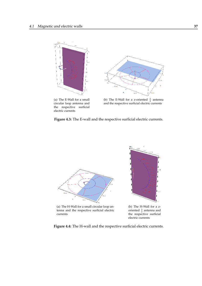
35
Chapter 4
E-wall , H-wall and Image theory
4.1 Magnetic and electric walls
Magnetic walls and electric walls (aka H-Walls and E-Walls) are merely explanatory mathematicaltools, that help us to understand the behavior of the fields. They are so ideal, that it were a realchallenge to manufacture H-Wall in reality. They are usually assumed planes or surfaces, whichpossess infinite dimension, and have total reflection and infinite electric conductivity as well.
Our convention states the following:
• E-Wall
– The only possible component of an Electric Field of a radiator, is the one which is normalto the surface, while the tangential components vanishes. (See Fig. 4.1)
– The only possible components of an Magnetic Field of a radiator, are the ones who aretangential to the surface, while the normal components vanish.(See Fig. 4.2(b))
– the electric field lines experience an odd symmetry with respect to their surface of sym-metry.
– the magnetic field lines experience an even symmetry with respect to their surface ofsymmetry.
– Magnetic Fields induce surficial electric currents on the surface of the E-wall. (See Fig.4.3)
– The surface is normal to the axis of the radiator, if the radiator is linear, otherwise it isparallel to it.

36 4 E-wall , H-wall and Image theory
(a) The electric field lines of a small circularloop antenna, the arrows show an odd sym-metry
(b) The electric field lines of z-oriented λ2
antenna, the arrows show an odd symme-try.
Figure 4.1: The electric fieldlines of a circular loop antenna 4.1(a) and a linear dipole 4.1(b)
(a) The magnetic field lines of a small circularloop antenna, the arrows show an odd sym-metry to the H-Wall
(b) The magnetic field lines of z-oriented λ2
an-tenna, the arrows show an odd symmetry tothe E-Wall.
Figure 4.2: The electric fieldlines of a circular loop antenna 4.2(a) and a linear dipole 4.2(b)
4.1 Magnetic and electric walls 37
(a) The E-Wall for a smallcircular loop antenna andthe respective surficialelectric currents
(b) The E-Wall for a z-oriented λ2
antennaand the respective surficial electric currents
Figure 4.3: The E-wall and the respective surficial electric currents.
(a) The H-Wall for a small circular loop an-tenna and the respective surficial electriccurrents
(b) The H-Wall for a z-oriented λ
2antenna and
the respective surficialelectric currents
Figure 4.4: The H-wall and the respective surficial electric currents.
38 4 E-wall , H-wall and Image theory
• H-Wall
– The only possible component of an Magnetic Field of a radiator, is the one which isnormal to the surface, while the tangential components vanish. (See Fig. 4.2)
– The only possible components of an Electric Field of a radiator, are the ones which aretangential to the surface, while the normal components vanish. (See Fig. 4.2(a))
– the electric field lines experience an even symmetry with respect to their surface of sym-metry.
– the magnetic field lines experience an odd symmetry with respect to their surface ofsymmetry.
– Electric Fields induce surficial magnetic currents on the surface of the H-Wall. (See Fig.4.3)
– The surface is either parallel to the axis of the radiator, or contains it, if the radiator islinear, otherwise it is normal to it.
4.2 Image Theory
E-Walls and H-Walls are surfaces of symmetry, where the fieldlines either start from certain pointson them, or land on other points. The start and landing points are separated by lines, whichwe call Border Contours ‘BC’. The existence of E-Walls and H-Walls as surfaces of symmetry forthe radiators, is essential if we were concerned in have closed loops as fieldlines. Due to thesymmetry, every half of these loops, is provides by one half of a symmetrically built radiator, whichis located at the origin.A dislocated radiator, or more generally an arbitrary oriented and located radiator, or even onewith complex construction, that has no symmetry, will certainly fail to produce closed loops asfieldlines.The Image theory, offers a great aid to cope with this very situation, and help us to analyze theperformance of a radiator. Every source has its counterpart image, that accounts for the reflectedreflection on the surface. These images are not real sources, but imaginary ones, which whencombined with the real sources, form an equivalent surface. This equivalent system gives thesame radiated field above the surface of symmetry as the actual system itself, for that below thissurface or within the field vanishes.
The amount of reflection is generally determined by the respective constitutive parameter belowand above surface of symmetry ‘SOS’. For a perfect electric surface (E-Wall) for instance, the entireincident wave will completely reflected, as the fields there vanish. According to the boundaryconditions, the tangential components of the electric field must vanish at all points along theinterface. The polarization of both the incident field, and that of the reflected wave must satisfythe boundary condition, in order to assume the right direction, in which currents flow in both of

4.2 Image Theory 39
the source and its image.
(a) The E-Wall for a small cir-cular loop antenna
(b) The E-Wall for a z-oriented λ2
antenna
Figure 4.5: The E-Wall for a small circular loop antenna and a linear one.
(a) The H-Wall for a small circularloop antenna
(b) The H-Wall for a z-orientedλ2
antenna
Figure 4.6: The H-Wall for a small circular loop antenna and a linear one.
This also valid for the (H-Wall). Important is, to observe the Boundary conditions as stated insection 4.1.For a single radiator located at the origin, the source and image coincide. Fig. 9.1 depicts the situ-ation, when an E-Wall is invoked, and Fig. 9.2 depicts the situation, when an H-Wall is invoked.
Now, if the center of the radiator is displaced by a distance z0 above the surface, an image at thesame opposite distance will be produced, the orientation of the currents of both source and image

40 4 E-wall , H-wall and Image theory
is shown in Fig. 9.3 showing the E-Wall.
(a) The E-Wall for a small cir-cular loop antenna, above is thesource and below is the image
(b) The E-Wall for a z-oriented λ2
antenna, the source and image
Figure 4.7: E-Wall, source and image for a small circular loop antenna and a linear one.
(a) The H-Wall for a small circularloop antenna, above is the sourceand below is the image
(b) The H-Wall for a z-oriented λ2
an-tenna, the source and image
Figure 4.8: H-Wall, source and image for a small circular loop antenna and a linear one.

4.2 Image Theory 41
Fig. 9.4 shows the H-Wall.
Eventually Fig. 9.5 depicts the situation for an arbitrary oriented dipole.
Radiators that have more complex construction like these, we just handled, could be like-wiselyturn into equivalent system of sources and images, just by following the same procedure as wementioned before.
(a) The E-Wall for a z-oriented λ2
antenna, the source and image(b) The H-Wall for a z-oriented λ
2
antenna, the source and image
Figure 4.9: E-Wall, H-Wall, source and image for a linear radiator.


43
Chapter 5
From EM Fields to fieldlines
What are the EM Fields?
They are vector functions, (1) who vary with respect to both spatial position ~r and time t. Theythus can in free space be expressed as
~E = ~E(t, ~r), ~D = ~D(t, ~r)~H = ~H(t, ~r), ~B = ~B(t, ~r)~r = ~r(x, y, z) (5.1)
where,~D = ε0~E ,~B = µ0
~H
When t varies, each of these vectors above traces out a curve, in general a space curve which variesin magnitude and direction, such a curve is called a hodograph.
The right side of both “Maxwell’s curl Equations”, ∇ × ~E = −∂ ~B∂t and ∇ × ~H = ∂ ~D
∂t , include time
derivative terms, that is, the rate of change of the “displacement current” ~D = ∂ ~D∂t with respect to
time and ~B = ∂ ~B∂t the rate of change of the “magnetic flux density” with respect to time.
For an instance of time ti, every point pi along the trajectories of the numerical integration of ~Dand ~B with respect to the time, can be express as
pi = p(ti, xi, yi, zi) |ti=const (5.2)

44 5 From EM Fields to fieldlines
Here we use a mathematical trick, by discretizing the time interval t, into chosen subintervals, eachof which, is fixed-valued, so Eq. (5.2) can be expressed in terms of the coordinates axes only, andone yet can trace the “time-varying factor” out.
pi = p(ti, xi, yi, zi) |ti=const = p(xi, yi, zi) |ti=const (5.3)
(a) The electric field lines loops of a z-oriented singlelinear Dipole lie in a meridian yz-plane, notice thatthe Boundary contour Dz = 0 lies in xy-plane. Evensymmetry to ‘IMS’, and odd symmetry to ‘IES’, ~n =0, 0, 1.
(b) The magnetic field lines loops of a z-oriented singlelinear Dipole lie in an equatorial xy-plane, notice thatthe Boundary contour By = 0 lies in xz-plane. Evensymmetry to ‘IES’, and odd symmetry to ‘IMS’, ~n =0, 1, 0.
Figure 5.1: The field lines and their symmetry surfaces
Plotting a series of many field lines, representing different ‘start points’ taken for consecutive subin-tervals each, will do the trick, to visualize quantities which vary with respect to ~r and t. Thedifference between Eq. (5.2) and Eq. (5.3) is obvious, the former requires a 4-orthogonal coor-dinate system, which is not invented yet, while the latter is very content with the familiar 3-orthogonal coordinate system. In addition the discretization is the core of all numerics, simplybecause the computer has only finite storage capacity, that will have hard times handling con-tinuous intervals, either in space or time, and hence there is no way to represent continuous data,except approximately as a sequence of discrete values. Using the rectangular coordinate system asa standard, has despite the inconvenience, the advantage to sum the vector fields of many radiators
up, besides its mostly the standard coordinate system in the simulation programs. Writing ~D and

45
~B in terms of their components, we come to a situation as shown in Fig. 9.2.
~D = Dx ~ex + Dy ~ey + Dz ~ez
~B = Bx ~ex + By ~ey + Bz ~ez (5.4)
~E = Ex ~ex + Ey ~ey + Ez ~ez~H = Hx ~ex +Hy ~ey +Hz ~ez (5.5)
Note The quantities in Eq. (5.4) lead their counterparts in Eq. (5.5) by Phase displacement of π2 due
to time-harmonic current distribution assumption.
Note Fig. 4.1 depicts the field lines and ‘SOS’ for a linear z-oriented Dipole located at origin, casewe have a small xy-loop antenna centered likewise, ‘IES’ and ‘IMS’ interchange their positions,and so also the ‘Electric’ and ‘Magnetic’ field lines, and their corresponding ‘Boundary contours’,
i.e., ~D → ~B and vice versa. Consider Fig. 4.1(a) and its counterpart Fig. 5.1(b), there an infinitesi-
mal segment d ~D and d ~B between two adjacent points p1 and p2 along their corresponding loops~D and ~B are respectively labeled. In terms of their components, they are
d ~D = dDx ~ex + dDy d~ey + dDz ~ez
d ~B = dBx ~ex + dBy ~ey + dBz d~ez (5.6)
The components dDx, dDy, dDy and dBx, dBy, dBy each represent spatial displacement, they eachcan be rewritten as dot product (·) of their gradients respectively, and a displacement vector d~r =dx ~ex + dy ~ey + dz ~ez
dDx = ∇(Dx) · d~r, dDy = ∇(Dy) · d~r, dDz = ∇(Dz) · d~r (5.7)
dBx = ∇(Bx) · d~r, dBy = ∇(By) · d~r, dBz = ∇(Bz) · d~r (5.8)
and
dDx = ∇(Dx) · d~r =∂Dx
∂xdx+
∂Dx
∂ydy +
∂Dx
∂zdz
= Φ1(Dx(t, x, y, z)) (5.9)

46 5 From EM Fields to fieldlines
dDy = ∇(Dy) · d~r =∂Dy
∂xdx+
∂Dy
∂ydy +
∂Dy
∂zdz
= Φ2(Dy(t, x, y, z)) (5.10)
dDz = ∇(Dz) · d~r =∂Dz
∂xdx+
∂Dz
∂ydy +
∂Dz
∂zdz
= Φ3(Dz(t, x, y, z)) (5.11)
Similarly
dBx = ∇(Bx) · d~r =∂Bx
∂xdx+
∂Bx
∂ydy +
∂Bx
∂zdz
= Ψ1(Bx(t, x, y, z)) (5.12)
dBy = ∇(By) · d~r =∂By
∂xdx+
∂By
∂ydy +
∂By
∂zdz
= Ψ2(By(t, x, y, z)) (5.13)
dBz = ∇(Bz) · d~r =∂Bz
∂xdx+
∂Bz
∂ydy +
∂Bz
∂zdz
= Ψ3(Bz(t, x, y, z)) (5.14)
The Equations (5.9) through (5.14) are functions of functions, each of which is a 4-dimensional func-
tion, however they all have their the dimensions of their fields, ~D and ~B respectively. These couldbe used whenever the field intensity is concerned. So that every field line can be associated witha certain strength, or intensity. To yield another sort of functions, however, i.e., functions witharguments in terms of x, y, z and t, we need to turn the equations (5.9) through (5.14) into di-mensionless ones. The trick is done by dividing them each by their corresponding vector-fieldmagnitude. Using another script, to show the new unit vectors:
d ~D =d ~D
|d ~D|= dDx~ex + dDy~ey + dDz~ez (5.15)
d ~B =d ~B
|d ~B|= dBx~ex + dBy~ey + dBz~ez (5.16)

47
where their corresponding components are
dDx =dDx
|d ~D|= f1(t, x, y, z), dDy =
dDy
|d ~D|= f2(t, x, y, z),
dDz =dDz
|d ~D|= f3(t, x, y, z) (5.17)
Equivalently we have
dBx =dBx
|d ~B|= g1(t, x, y, z), dBy =
dBy
|d ~B|= g2(t, x, y, z),
dBz =dBz
|d ~B|= g3(t, x, y, z) (5.18)
These six quantities represent four dimensional differential equation each, these have to be solvedsimultaneously, for the values of x, y, z and t, where as we mentioned above only fixed values oft are admissible, the algorithm form the values for the points on the integration path in form ofpi = p(x, y, z) |t=const, accumulate then in lists, coded them, then use them in plotting.


49
Chapter 6
Start points for line tracing
Although start points must be found in magnetic and electric walls as well, the following explana-tion shall be given for the perfectly conducting plane. Here the surface currents do indeed exist,in the other planes they have to be derived from the field. So the more familiar scenario is invokedfor purposes of explanation.
6.1 Topology of surface and displacement currents
Currents in perfectly conducting surfaces are two dimensional vector fields, here in the x,y-plane.In a time harmonic field each of the two components Jx and Jyvanishes along a curve for a giventime. The intersections of both curves define points of zero current density, called PZD in thefollowing.
Jx = 0, Jy = 0
Under normal conditions the magnetic field above metallic surfaces shows an elliptical polariza-tion. Due to ~J = ~n× ~H, this holds true for the current density ~J too. Along certain lines - the linesof linear polarization - the polarization ellipses degenerate into straight lines. So the current canvanish only at these lines, PZD can be found only here.
Now the border contour ‘BC’ between starting and landing regions can be determined. Keepingin mind the complex formulation jωDz , the time dependent formulation is given by:
Dz = <(jωDz) cos(ωt)−=(jωDz) sin(ωt) (6.1)

50 6 Start points for line tracing
So vanishing values for an arbitrary time t1 are given by:
tan(ωt1) =<(jωDz)=(jωDz)
−→ −ωt1 = arctan(=(Ez)<(Ez)
)±nπ (6.2)
In the past, the lines of constant amplitude and constant phase were widely used to characterizethe time harmonic electric field above metallic surfaces. They could be easily measured with amonopole probe and a vector voltmeter.
|Ez|2 = =2(Ez) + <2(Ez) arg(Ez) = arctan(=(Ez)<(Ez)
)(±π) (6.3)
As the arctan function is normally defined over [−π · · ·+ π], however, the phase angle π has to beadded or subtracted depending on the quadrant.
Comparing the equations (6.3) and (6.2) shows that the BC for a given time t1 can be referred tothe phase front:
arg(Ez) = −ωt1(±π) (6.4)
6.1.1 Discretization of the conducting plane
The tracing of the BC’s can be started from any arbitrary point ‘Start’ in the ‘SOS’ Fig. 6.1, whereDz = 0 holds true. Integrating the magnetic field along the BC with the coordinate s yields thecurrent I , crossing the BC between the start and any other point of the path.
Figure 6.1: Border contours with the region of interest and current lines

6.1 Topology of surface and displacement currents 51
(a) Sector, subdivided into ar-eas launching the same displace-ment current
(b) Fieldlines, embedded insurfaces of constant I or con-stant ζ, forming horizontalor vertical families
(c) Field line, appearing or disappearing at a BC
Figure 6.2: Regions of interest, border contours, sectors and field lines
I =
s1∫Start
~Hd~s =
s1∫Start
~n× ~Jd~s (6.5)
Now the area of interest can be indicated by Imax.
Imax =
Stop∫Start
~Hd~s =
Stop∫Start
~n× ~Jd~s (6.6)
Segmentation of the BC between ’Start’ and ’Stop’ into N parts with the same amount of crossingcurrents ∆I = Imax/N divides the total current into equal portions ∆I .
Now the flow lines of Fig.4.3(b) can be started, all parallel to the surface current density vector ~J .

52 6 Start points for line tracing
They usually end in a PZD. The current i enclosed between two lines is given by:
i = | ~J | · sinα · w (6.7)
The conduction current I gradually becomes the displacement current, stemming from the plane.The continuity equation requires that the amount of displacement current, launching from thedashed area w sinα∆η in Fig.6.2(a) is equal to the difference between the currents i entering at η1
and leaving at η2 :
∂i
∂η·∆η = − ∂
∂η(| ~J | sinαw)∆η = w sinα∆η · Dz (6.8)
Eq.(6.8) shows, that the maximum of i occurs in the BC, where Dz = 0.
The next task is to subdivide the area 1, 2, PZD in Fig.6.2(a) into pieces, from which the sameamount of displacement current arises. A helpful tool to this end can be a second vector field ~j inthe plane, which is parallel to ~J everywhere, but divergence-less,
~j = g(x, y) · ~J (6.9)
Now a new fictive current i, crossing the lines η = const. can be referred to
i = |~j(η)| · sinα · w = ∆I
which does not depend on η.
Extending the term in brackets in eq.(6.8) by the function g defined in eq. (6.9) yields after differ-entiation:
− ∂
∂η
(g| ~J | sinαw1
g
)·∆η = −1
g
∂
∂η
(g| ~J | sinαw
)·∆η +
1g2
∂g
∂η(g| ~J | sinαw) ·∆η
The first differentiation on the right side leads to zero, as i = g| ~J | sinαw is independent of η.Together with eq. (6.8):
Dzw sinα∆η =1g2
∂g
∂η(g| ~J | sinαw) ·∆η

6.1 Topology of surface and displacement currents 53
Rearranging makes a direct integration on either side possible:
Dz
| ~J |=
1g
∂g
∂ηln g =
η∫η=0
Dz
| ~J |dη (6.10)
Now a re-scaling of the η coordinate can be done in such a way, that the remaining current i(η) =∆I/g in the sector is normalized ∆I .
Starting from the BC and keeping in mind that g(η = 0) = 1 results in
ζ = (1− 1/g) (6.11)
with the new scaling ζ from 0 at the BC to 1 in the PZD.
6.1.2 Line families
Up to now the area of interest has been defined and divided into sectors, starting from a BC.Another division of these sectors into subareas, each launching the same displacement current,led to the start points for field lines. These could be placed in the middle of the subareas or, likedone here, in the intersection points of the coordinate lines of I and ζ of the new skew coordinateframe for the area of interest.
Once the displacement currents lines have been calculated, the values of I and ζ can be transferredfor all points in the volume of interest above the plane. So I = const. and ζ = const. in Fig.6.2(b)describe bunches of surfaces, in which lines are embedded. So the lines can be assumed again asan intersection of two surfaces, as it has been done in the 2nd section for the simple cases. So eachline can be associated to the values of I and ζ of its start point. On the other hand, two differentgroups or families can be distinguished: lines, starting from points with constant I lead to a groupof lines, we call horizontal family. Starting from points with constant ζ, leads to a vertical family.
6.1.3 Chronological visualization of the field evolution
The basis of an animated film are frames, i.e. field plots following one another. The questiontherefore arises as to a line can be referred to another in a plot for an earlier as well as later time.To answer this question, one should regard the ‘birth‘ or ‘death‘ of a line, the limits of its ‘life‘,

54 6 Start points for line tracing
which can occur on BCs only. In Fig.6.2(c) a field-line in the vicinity of a BC is shown at threedifferent times t1, t2, t3. For t1 < t2 < t3 a line appears, for t1 > t2 > t3 a line disappears.
Consider a BC at two different times, the start time t0 and an arbitrary time whereby t > t0. Theresults for Imax calculated with eq. (6.6) for both times will be different most probably. Proceedingas described above would lead to different ∆I . The pieces however, in which the sector 1,2,PZDhas to be divided, must launch the same amount of displacement current at both times. So theremaining current i(η) must not be normalized w.r.t. different ∆I , but only w.r.t. ∆I(t0) for bothtimes t0 and t, whereas the number N has to be held constant.
As the lines appear or disappear on the BC, a new scale ζ instead of ζ appears expedient, beginningin the PZD with ζ = 0 and ending at the BC.
ζ =∆I(t)∆I(t0)
· 1g
=∆Imax(t)∆Imax(t0)
· 1g
0 < ζ <∆I(t)∆I(t0
Keeping the number N for both times is easy to enforce for a closed BC. The maximum of ζ,ζmax = ∆I(t)/∆I(t0) determines whether lines appear (ζmax > 1) or disappear (ζmax < 1)
6.1.4 The new surface definitions, applied to a straight wire
It is worth to formulate the new surface definition to the rotational symmetric case of a straightfilament current with a symmetry to the xy-plane . With
I =∫
~Hd~s =
φ0∫φ=0
Hφ(Dz = 0) · ρdφ
one gets an integration path with constant ρ the path element ds = ρdφ and constant values of Hφ.So ρHφ can be taken out of the integral.
I = ρHφ
∣∣∣∣Dz=0
φ0∫φ=0
dφ = ρ0Hφ(ρ0)φ0 (6.12)
where the index 0 denotes a radius where Dz = 0. So, planes of constant φ are the first group.

6.1 Topology of surface and displacement currents 55
The second is given by constant values of ζ or, closer to the original calculation, of g, given by eq.(6.10). With Dz, | ~J | and the path element dη in the cylindrical coordinates one obtains
Dz =1ρ
∂
∂ρ
(ρHφ
)|J | = Hφ dη = dρ
due to symmetry. So eq. (6.12) becomes:
ln g =
ρ∫ρ=ρ0
1ρHφ
∂
∂ρ
(ρHφ
)dρ = ln
(ρHφ
)∣∣∣∣ρρ0
g =ρHφ(ρ)ρ0Hφ(ρ0)
= ρHφ(ρ) · const.


57
Chapter 7
On the arbitrarily oriented radiators
Dr. Zuhrt H. (5) in his book “Electromagnetic radiation fields”, Springer 1953”, seems to be theonly one, sofar, who made an attempt to deal the general case of orientation, he described a rathersimple method to derive a formula, unfortunately, that method covers but the Far-Field of a hori-zontally oriented Hertzian.
Though we are grateful to his revolutionary advance, indeed, it was not at all satisfactory, firstfor that he considered the far-field case only, and finally, that he restricted it on just a Hertzian.The Hertzian Dipole, though of some scientific interest to understand the behavior of more com-plicated antennas, is by no means a real antenna that could exist for its own. It is nothing morethan a piece of uniform current of infinitesimal length, that is. This chapter presents a techniqueused to derive the entire field formulas for both arbitrary oriented Hertzian and finite length lin-ear Dipoles, and visualize the electric and magnetic field lines, afterwards. The arbitrary orientedhalf-wave linear dipole though, will be taken as a standard example for convenience.
One encounters such a dipole in all imaginable orientation, in almost every aspect, that has any-thing to do with broadcasting, transmitting or receiving signals, either in the free space or underthe sea. Sometimes, one finds such a dipole in a stationary variant, like being a part of a com-plicated radiating object, or also in a transient variant, that change its orientation continuously,just consider a jet or a submarine, tracing certain courses. Now, as it is obviously clear, that such adipole is significant, how comes that everybody left it over? The reason, obviously, is the difficultyto derive its formulas in the conventional manner, besides, there is always alternatives for every-thing in life, an arbitrary oriented dipole antenna, can also be replaced be weighted dipoles, thatone is accustomed with their formulas and radiation, with the suitable combination of these, onecan get the equivalent of an arbitrary oriented. It works, but whence it gets to closed field linesvisualization, the entire process will certainly collapse, simply because having an equivalent outof three other dipoles oriented in the direction of the three axes, has no symmetry plane, and thusthe enclosure of these lines won’t occur. For this very reason, we were very concerned in deriving

58 7 On the arbitrarily oriented radiators
formulas belong to a real arbitrary oriented, not its substitute.
7.1 A provoked solution: Replacement Rules
Four years ago, we came out with a simple and very efficient solution that deals with dipoles,which are oriented in the other axes rather the z-axis. Astonishingly this process worked fine withall sort of the dipoles considered, i.e., they do not have to be of linear form. The solution was todevelop some replacement rules, applied to the formulas of a Z-oriented antenna, to get in no timenew formulas for the desired orientation to either of the other rectangular coordinates, that is, Xor Y.
How does it really work?
Let’s explain the process briefly right here. We will furthermore adopt mathematica notation toexpress, vectors, sets and replacement rules, to keep as close as possible, to the items used inthe programs used to visualize the results. Consider first, the following three sequences of thecoordinates system, X, Y, and Z, Y, Z, and X, Z, X, and Y . At once, one will notice thatthey are the rotations of each other, in a positive sense of the right hand rule. Fig.7.1 on page 58depicts the situation.
(a) X Y Z (b) Y Z X (c) Z X Y
Figure 7.1: Rotating Coordinates
Now, notice the last symbol of each sequence, and compare this to its own axes in figure 1, amaz-ing, all we need is, in the axes in Fig. 7.1(b), z replaced by X, X by Y, and Y by Z, and in Fig.

7.1 A provoked solution: Replacement Rules 59
7.1(c) to the right Z replaced by Y, Y by X, and X by Z, right? And exactly these our replacementrules, that we apply to the formulas of a Z-oriented dipole to obtain either an X orientation or a Yorientation, by applying the set of rules belongs to the desired orientation.In other words: To derive formulas for an X oriented antenna from, old formulas derived for aZ oriented one, do the following:
¬ Replace all X’s in an expression by Y’s or in mathematica notation x :→ y
Replace all Y’s in an expression by Z’s or in mathematica notation y :→ z
® Replace all Z’s in an expression by X’s or in mathematica notation z :→ x
Or just follow the following steps instead to derive formulas for an y-oriented antenna from, oldformulas derived for a z-oriented one, do the following:
¬ Replace all X’s in an expression by Z’s or in mathematica notation x :→ z
Replace all Y’s in an expression by X’s or in mathematica notation y :→ x
® Replace all Z’s in an expression by Y’s or in mathematica notation z :→ y
Quite elementary, isn’t? We though, decided to be completely sure of the correctness of theserules, so we derived, in conventional method, the formulas for the X and Y oriented antennas,and the comparison showed that the results were identical, a matter that, we never doubtedactually. The technique, in reality, based on simple and elegant concept, that is, always create anew coordinates system, where the dipole antenna keeps its Z orientation, but in terms of thenew belonging to coordinates.
In other words, we simulate a new up-down world for the dipole in which, only the dipoleitself, believes that it were Z oriented, to the old coordinates system. That’s true, case it take therole of an X oriented, the X axis of Y, Z, X system coincides with the Z axis of X, Y, Zsystem, and the dipole will radiate further, without noticing the drastic changes, of the orientation.
7.1.1 Limitations
However, though these rules were very effective in time and efforts’ sparing, they were not verysatisfactory to us; we wanted to extend them further to cover real arbitrary cases, many methodswere considered, and finally we decided for Euler’s rotation theorem, it is the most straightfor-ward approach to our method, and it is besides its simplicity to be understood and programmeda very effective tool too.

60 7 On the arbitrarily oriented radiators
7.2 Rotation Matrices
According to Euler’s theorem of rotation, any rotation can be described using three angles, namelya triple (ϕ, ϑ, ψ). Each of these rotations can be written and described in terms a rotation matrix,and then a general matrix A, which is the multiplication of all the three matrices, can be con-structed. Unfortunately, there are several conventions for Euler angles, depending on the axesabout which the rotations are carried out. One can obtain 12 different rotation sequences; onlythree of them are widely used, in graphics and computer games or simulators.
7.2.1 The Adopted Rotation Matrix
The so-called “x-convention”, is the most common definition. In this convention, the rotationgiven by Euler angles (ϕ, ϑ, ψ), where the first rotation is by an angle ϕ about the z-axis, thesecond is by an angle ϑ about the x-axis, and the third is by an angle ψ about the z-axis (again).
Note, however, that several notational conventions for the angles are in common use. Gold-stein (7)(1960, pp. 145-148) and Landau and Lifschitz (1976) (8)use (ϕ, ϑ, ψ), Tuma (1974) (11)says (ψ, ϑ, ϕ) is used in aeronautical engineering in the analysis of space vehicles (but claims that(ϕ, ϑ, ψ) is used in the analysis of gyroscopic motion), while Bate et al. (1971) use (Ω, ι, ω) . Gold-stein remarks that continental authors usually use, and warns that left-handed coordinate systemsare also in occasional use (ψ, ϑ, ϑ)(Osgood 1937 (10), Margenau (9)). Varshalovich (12)(1988, pp.21-23) uses the notation (α, β, γ) or (α′, β′, γ′) to denote the Euler angles, and gives three differentangle conventions, none of which corresponds to the x-convention. No matter, we will describeand use, the x- convention, a.k.a ZXZ convention.Let’s call the first rotation about the Z axis Rz(ϕ), and the second rotation about the rotated X-axis(X’) Rx(ϑ), and finally the third and last rotation about the rotated Z-axis(Z’) Rz(ψ). Thedefinition of Rz(ϕ) is given by:
Rz(ϕ) =
cos(ϕ) sin(ϕ) 0− sin(ϕ) cos(ϕ) 0
0 0 1
(7.1)

7.2 Rotation Matrices 61
Figure 7.2: A Z-oriented Dipole centered at origin, along with its electric symmetry plane!
Applying this Rotation Matrix Rz(ϕ) to a Z-Oriented linear dipole 7.2, it results in that, the X-axisand Y to rotate clockwisely about the Z-axis by an angle ϕ, Fig.7.3 depicts its effect:
Figure 7.3: The first Rotation about Z-axis!
The primed symbols indicate that a rotation has taken place.The next rotation Rx(ϑ) that follows the first one immediately, is about the rotated X-axis (X’)byan angle ϑ and given by:
Rx(ϑ) =
1 0 00 cos(ϑ) sin(ϑ)0 − sin(ϑ) cos(ϑ)
(7.2)
Fig.7.4 depicts its effect:

62 7 On the arbitrarily oriented radiators
Figure 7.4: The second Rotation about X’-axis!
The last rotation that follow is about the rotated Z-axis (Z’) by an angle ψ and given by Rx(ψ)Rotation Matrix:
Rz(ψ) =
cos(ψ) sin(ψ) 0− sin(ψ) cos(ψ) 0
0 0 1
(7.3)
Its final effect results in the desired orientation of the dipole, as the depicted in Fig.7.5. Note thedouble prime of the symbols now.Now we have got a dipole, which orientation coincides with Z”, which match exactly the desiredorientation, we had in mind, i.e., expressed in terms of Euler triple (ϕ, ϑ, ψ).
Figure 7.5: The third Rotation about Z’-axis!
The three successive rotations can be expressed in terms of one general rotation matrix A, which

7.2 Rotation Matrices 63
is their multiplication, as given by Equation 4.
A = Rz(ψ) ·Rz(ϑ) ·Rz(ϕ) (7.4)
This can be written in terms of a matrix
A =
a11 a12 a13
a21 a22 a23
a31 a32 a33
(7.5)
where
a11 = cos(ψ) cos(ϕ)− cos(ϑ) sin(ϕ) sin(ψ)a12 = cos(ψ) sin(ϕ) + cos(ϑ) cos(ϕ) sin(ψ)a13 = sin(ψ) cos(ϑ) (7.6)
a21 = − sin(ψ) cos(ϕ)− cos(ϑ) sin(ϕ) cos(ψ)a22 = − sin(ψ) sin(ϕ) + cos(ϑ) cos(ϕ) cos(ψ)a23 = cos(ψ) sin(ϑ) (7.7)
a31 = sin(ϑ) sin(ϕ)a32 = − sin(ϑ) cos(ϕ)a33 = cos(ϑ) (7.8)
Rotation matrices are orthogonal matrices, i.e. unit matrices (which are matrices for which M ·MT = I) with real coefficients. The module of the determinant of unit matrices is one, among theorthogonal 3× 3 matrices, only the ones having a positive determinant (+1) are rotation matrices.Notice we used the transpose of a matrix instead of its inverse, simply because, their determinantwere the unity.
One notes that our replacement-rules were, intuitively and implicitly based on Euler’s angles
principal. For a Z-oriented Dipole, we set ϕ = ϑ = ψ = 0. The A matrix attributed to this
orientation is A =(
1 0 00 1 00 0 1
), to obtain an orientation in the x-Axis, we just set ϕ = 0, ϑ = 3π
2 and ψ =
3π2 instead, to obtain A =
(0 1 00 0 11 0 0
). The y-orientation is easily obtained, likewise, by setting ϕ =
π2 , ϑ = π
2 and ψ = 0, and thus A =(
0 0 11 0 00 1 0
).
7.2.2 What are transpose Matrices really good for?
The transpose of a matrix A is a matrix formed from A by interchanging the rows and columnssuch that row i of matrix Abecomes column i of the transposed matrix. The transpose of A is

64 7 On the arbitrarily oriented radiators
denoted by AT . Each element aij in A becomes element aji in AT . The following represents AT
the transpose of A:
AT =
a11 a21 a31
a12 a22 a32
a13 a23 a33
(7.9)
Rotating a dipole implies rotating its field along with its orientation. Multiplying the rotation
matrix A by the vector, containing the original coordinates, say ~X =
(xyz
), will invoke the
replacement rules, ~X ′ = A · ~X =
(x′
y′
z′
)these when applied to a field vector, e.g., the magnetic
vector ~H = Hx ~ex + Hy ~ey + Hz ~ez , or in vector notation ~H =
(Hx
Hy
Hz
)will result in a vector field
~H ′ =
H ′x′
H ′y′
H ′z′
, these expressions though completely correct in content and symbols, they have al-
together different order: H ′x′ , H
′y′ , H
′z′ refer to their corresponding new coordinates,X ′, Y ′, Z ′
they are by no means, components of the old world of X, Y, Z.
Is that a real problem? Certainly not to a human, but for a machine that is programmed, to dealmatters sequentially, it is a serious problem. Quite often, one has a sophisticated software writtento simulate a real 3D world, like ours, and its by convention that x-component been placed first,followed by y-component and finally z-component, to visualize the fields lines belong to the neworientation, we must rearrange the component within the new vector, that they match the oldorder. Otherwise, the visualization will make no difference from those the z-oriented one.
A correction
The multiplication by AT the transpose of A corrects this behavior and produces a new vector
~H = Hx ~ex +Hy ~ey +Hz ~ez , or as vector ~H = AT ·
H ′x′
H ′y′
H ′z′
=
Hx
Hy
Hz
, so the calligraphic text is
right here reserved for the corrected fields.
The next installment To Formulas deals the matter of more details, and finally gives expressions forthe arbitrary oriented dipole for both a Hertzian and finite length dipole.

7.3 To Formulas 65
7.3 To Formulas
Now, in the XYZ system, a space vector ~r from the origin to the point of observation P in the spacecan be expressed as
~r = x~ex + y~ey + z~ez (7.10)
and its magnitude is
r = |~r| =√x2 + y2 + z2 (7.11)
in the X’Y’Z’ system (see Fig. 7.6), however, the very same vector is defined by
~r′ = x′~e ′x + y′~e ′y + z′~e ′z (7.12)
Figure 7.6: Two coordinates systems!
Thought they both obviously have the very same magnitude r = r′ =√x2 + y2 + z2, we have
e.g., x 6= x′, y 6= y′, z 6= z′, ~ex 6= ~e ′x, ~ey 6= ~e ′y,& ~ez 6= ~e ′z . To distinguished between the different casesof orientation, we are making a convention by reserving the unprimed symbols for the case of aZ-oriented cases, primed otherwise.We just agreed that original non-rotated coordinates can be expressed in a vector notation as ~X =(XYZ
), the rotated one is ~X ′ =
(X ′
Y ′
Z ′
), so that every point in space ~P (x, y, z) can be expressed in
both coordinates systems components equivalently as
(x′
x′
z′
)= A ·
(xyz
)or
(xxz
)= AT ·
(x′
y′
z′
).
Table # 7.1 summarizes the entire replacement rules used in this work. We will show a sign of

66 7 On the arbitrarily oriented radiators
courtesy to mathematica, that helped us doing the visualizations though, by adopting its notation,so the symbol slash dot (/·) will be used as a replacement operator.
In X Y Z System In X’ Y’ Z’ Systemx = a11x
′ + a21y′ + a31x
′ x′ = a11x+ a12y + a13zx = a12x
′ + a22y′ + a32x
′ x′ = a21x+ a22y + a23zx = a13x
′ + a23y′ + a33x
′ x′ = a31x+ a32y + a33z
Table 7.1: Replacement rules
Applying a set of rules, let’s say x :→ x′ y :→ y′ z :→ z′ on either an electric field vector
~E =
Ex
Ey
Ez
or a magnetic field vector ~H =
Hx
Hy
Hz
, rotates the fields and induces
~E / · x :→ x′ y :→ y′ z :→ z′ = ~E′ =
(E′
x
E′y
E′z
)
and ~H / · x :→ x′ y :→ y′ z :→ z′ = ~H ′ =
(H ′
x
H ′y
H ′z
)respectively. Table # 7.2 shows that every
new field component is indeed a combination of all the three old components, weighted by thecorresponding component of the rotation matrix A.
Magnetic field components Electric field componentsH ′
x = a11Hx + a12Hy + a13Hz E′x = a11Ex + a12Ey + a13Ez
H ′x = a21Hx + a22Hy + a23Hz E′x = a21Ex + a22Ey + a23Ez
H ′x = a31Hx + a32Hy + a33Hz E′x = a31Ex + a32Ey + a33Ez
Table 7.2: The rotated fields components
The next example will show that these components, though completely correct symbolically, theirorder won’t satisfy a machine, a robot for instance, or another program, that used to work on setsof input data, which come in a certain order.

7.3 To Formulas 67
An example
To keep the discussion as simple and obvious as possible, we will consider a magnetic field vec-tor of a Z-oriented linear dipole regardless of its sort. It has no magnetic component along its
axis or Hz = 0, so the magnetic field vector reduces to ~H =
Hx
Hy
0
, we furthermore want to
extract expressions for an X-oriented dipole, and have, therefore, constructed a rotation matrix
A =
0 1 00 0 11 0 0
and its transpose AT =
0 0 11 0 00 1 0
. The coordinates of any point P (x, y, z) in space
can expressed in terms of newly generated coordinates by
(x′
y′
z′
)=
(0 1 00 0 11 0 0
)·
(xyz
)=
(yzx
)in
space can expressed in terms of newly generated coordinates by
(yzx
), and so the magnetic field
that yields ~H ′ =
(0 1 00 0 11 0 0
)·
(Hx
Hy
0
)=
(Hy
Hz
0
), this is indeed expressions for an X-Oriented dipole
alright, for that the Hx vanishes, but the order of the components is not satisfactory.
Now multiply ~H ′ by AT corrects the order, as we desire it: ~H =
Hx
Hy
Hz
=
0 0 11 0 00 1 0
·
Hy
Hz
0
=
0Hy
Hz
Now its been done!
Yet another example
Now, we want to extract a Y-oriented Dipole out of the wellknown Z-oriented formulas, and
have, therefore, constructed a rotation matrix A =
0 0 11 0 00 1 0
and its transpose AT =
0 1 00 0 11 0 0
.
The coordinates of any point P (x, y, z) in space can expressed in terms of newly generated coor-
dinates by
(x′
y′
z′
)=
(0 0 11 0 00 1 0
)·
(xyz
)=
(zxy
)in space can expressed in terms of newly generated
coordinates by
(zxy
), and so the magnetic field that yields ~H ′ =
(0 0 11 0 00 1 0
)·
(Hx
Hy
0
)=
(Hz
Hx
0
), this

68 7 On the arbitrarily oriented radiators
is, once more, indeed expressions for an Y-Oriented dipole alright, for that the Hy vanishes, butthe order of the components is not satisfactory.
Now multiply ~H ′ by AT corrects the order, as we desire it: ~H =
Hx
Hy
Hz
=
0 1 00 0 11 0 0
·
Hz
Hx
0
=Hx
0Hz
To cover the case of dealing an arbitrary oriented linear finite length radiating object as well, thedistance from each tip (please see Fig. # 7.7) has got to be defined as in table 7.3 on page # 68.
Figure 7.7: Dimensions for a finite length linear dipole!
Z-oriented Arbitrary Oriented
R1 =√x2 + y2 + (z − `
2)2 R′1 =√x′2 + y′2 + (z′ − `
2)2
R2 =√x2 + y2 + (z + `
2)2 R′2 =√x′2 + y′2 + (z′ − `
2)2
Table 7.3: two more dimensions for a finite length

7.3 To Formulas 69
7.3.1 For an arbitrarily oriented Hertzian Dipole
magnetic fields
Hx = I0 d`
4π
((−a11y
′ + a21x′
r′3
)+ β
(−a11y
′ + a21x′
r′2
))e− β r′ (7.13)
Hy = I0 d`
4π
((−a12y
′ + a22x′
r′3
)+ β
(−a12y
′ + a22x′
r′2
))e− β r′ (7.14)
Hz = I0 d`
4π
((−a13y
′ + a23x′
r′3
)+ β
(−a13y
′ + a23x′
r′2
))e− β r′ (7.15)
The amazing matter, that a new componentHz has appeared right from a blue sky! Remember nodipole has a magnetic component along it axis.
In analogous way we go ahead to derive the corresponding expressions of the electric fields:
Electric Fields
Ex =I0 d`
4π ω ε
((3z′(a11x
′ + a21y′) + a31(3z′2 − r′2)r′5
)+ β
(3z′(a11x
′ + a21y′) + a31(3z′2 − r′2)r′4
)− β2
(z′(a11x
′ + a21y′) + a31(z′2 − r′2)r′3
))e− β r′ (7.16)
Ey =I0 d`
4π ω ε
((3z′(a12x
′ + a22y′) + a32(3z′2 − r′2)r′5
)+ β
(3z′(a12x
′ + a22y′) + a32(3z′2 − r′2)r′4
)− β2
(z′(a12x
′ + a22y′) + a32(z′2 − r′2)r′3
))e− β r′ (7.17)

70 7 On the arbitrarily oriented radiators
Ez =I0 d`
4π ω ε
((3z′(a13x
′ + a23y′) + a33(3z′2 − r′2)r′5
)+ β
(3z′(a11x
′ + a21y′) + a33(3z′2 − r′2)r′4
)− β2
(z′(a13x
′ + a23y′) + a33(z′2 − r′2)r′3
))e− β r′ (7.18)
7.3.2 For an arbitrarily oriented finite length linear dipole
Magnetic Fields
Hx = I0 (−a11y
′ + a21x′)
4π(x′2 + y′2)
(e− β R′
1 + e− β R′2 − 2 cos
(β `
2
)e− β r′
)(7.19)
Hy = I0 (−a12y
′ + a22x′)
4π(x′2 + y′2)
(e− β R′
1 + e− β R′2 − 2 cos
(β `
2
)e− β r′
)(7.20)
Hz = I0 (−a13y
′ + a23x′)
4π(x′2 + y′2)
(e− β R′
1 + e− β R′2 − 2 cos
(β `
2
)e− β r′
)(7.21)
Electric Fields
Ex = η I0
4π(x′2 + y′2)
((e− β R′
1 + e− β R′2 − 2 cos
(β `
2
)e− β r′
)∗
((a11x
′2 + a21y′2)− a31
(x′2 + y′2
)))(7.22)
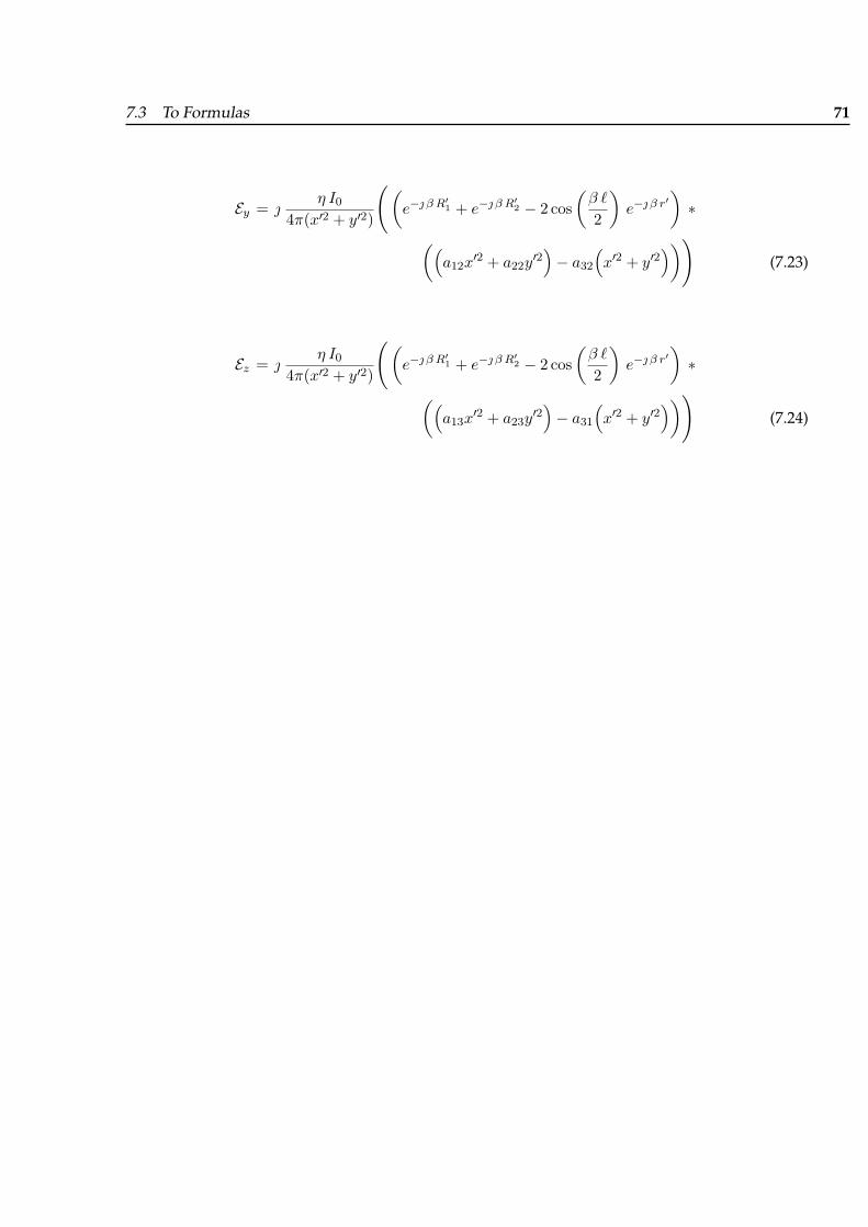
7.3 To Formulas 71
Ey = η I0
4π(x′2 + y′2)
((e− β R′
1 + e− β R′2 − 2 cos
(β `
2
)e− β r′
)∗
((a12x
′2 + a22y′2)− a32
(x′2 + y′2
)))(7.23)
Ez = η I0
4π(x′2 + y′2)
((e− β R′
1 + e− β R′2 − 2 cos
(β `
2
)e− β r′
)∗
((a13x
′2 + a23y′2)− a31
(x′2 + y′2
)))(7.24)


73
Chapter 8
Numerical Approach
NUMERICAL solution of ordinary differential equations is the most important technique in con-tinuous time dynamics. Since most ordinary differential equations are not soluble analytically,numerical integration is the only way to obtain information about the trajectory. Many differentmethods have been proposed and used in an attempt to solve accurately various types of ordinarydifferential equations. However there are a handful of methods known and used universally (i.e.,Runge-Kutta, Adams–Bashforth–Moulton and Backward Differentiation Formulae methods). All thesediscretize the differential system to produce a difference equation or map. The methods obtaindifferent maps from the same differential equation, but they have the same aim; that the dynam-ics of the map should correspond closely to the dynamics of the differential equation. From theRunge–Kutta family of algorithms come arguably the most well-known and used methods fornumerical integration.
Differential equation is an equation involving an unknown function and one or more of its deriva-tives. The equation is an ordinary differential equation (ODE) if the unknown function dependson only one independent variable.
As for numerical methods, bear the following items in mind:
( Solution of a DE is function in infinite-dimensional space.
( Numerical solutions of a DE is based on finite-dimensional approximation.
( Differential equation is replaced with algebraic equation, called Difference equation whoseapproximates that of given DE.
( There is no method, which can deliver the best results, all times.
With a differential equation, we can associate initial conditions or boundary conditions, auxiliary
74 8 Numerical Approach
conditions on the unknown function and its derivatives. If these conditions are specified at a singlevalue of the independent variable, usually at start points, they are referred to as initial conditionsand the combination of the differential equation and an appropriate number of initial conditions iscalled an initial value problem (IVP). If these conditions are specified at more than one value of theindependent variable,usually at start and end points, they are referred to as boundary conditionsand the combination of the differential equation and the boundary conditions is called a boundaryvalue problem (BVP). Partial differential equations are beyond the scope of this text, instead we shalltake a brief look at some methods for solving the single first-order ordinary differential equation,written in the standard form:
y′ = f(x, y) (8.1)
we expand the scope of eq (8.1) to cover a system of differential equations in section 8.2.
A minimal requirement
The functions we shall be considering here when discussing the implemented numerical methodsone by one, are assumed to be continuous, since this is a minimal requirement for predictablebehavior. The set of formulas, in hand may have derivatives of all orders as well C∞(X), andnon-stiff equations as well, so it is just right to adopt methods used to solve the IVPs, to solve themnumerically.
Functions that are not continuous can skip over point of interest, which is not satisfactory traitwhen attempting to approximate a solution. More sophisticated understanding of the nature ofa problem, leads to a better formulation, in our Test Problem in section 8.2.1 on page 86, we triedto give a comprehensive description of the Kepler’s Problem, which has been chosen, due the fact,that it is very sensitive to the initial conditions, therefore, once the used algorithms succeed there,they will also succeed in solving much well-posed set of formulas.
A well-posed Problem
The term well-posed problem stems from a definition given by French mathematician J. S.Hadamard. He believed that mathematical models of physical phenomena should have the prop-erties that:
A good method possesses the following three characteristics:
Ê A solution exists.
Ë The solution is unique ( that is, there is one and only one solution to the differential equa-tion).

75
Ì The solution depends continuously on the data, in some reasonable topology. Topology isthe study or science of places.
If a problem is well-posed, then it stands a good chance of solution on a computer using a stablealgorithm. If it is not well-posed, it needs to be re-formulated for numerical treatment. Typicallythis involves including additional assumptions, such as smoothness of solution. This process isknown as regularization, which means making a function regular or smooth. A smooth functionis one that is infinitely differentiable, i.e., has derivatives of all finite orders.
In the course of carrying out a mathematical computation, one has to deal with problem of errors.There are three ways in which errors can enter a calculation.
Sources of error
The main sources of error in obtaining numerical solutions to mathematical problems are:
1 The model: its construction usually involves simplifications and omissions;
1 The data: there may be errors in measuring or estimating values;
1 The numerical method : generally based on some approximation (truncation);
1 The representation of numbers: (roundoff) for example,π cannot be represented exactly bya finite number of digits;
1 The arithmetic: frequently errors are introduced in carrying out operations such as addition(+) and multiplication (∗) .
Each of these errors is unavoidable in a calculation. Hence, the “problem of errors” is not one ofpreventing their occurrence. Instead, it is one of controlling their size in order to obtain a finalresult that is as accurate as possible. This process is called error control. It is concerned withthe propagation of errors throughout a computation. For example, we want to be sure that theerror that results from performing an arithmetic operation on two or more numbers, which arethemselves in error, is within tolerable limits. In addition, the propagation or cumulative effects,of that error in subsequent calculations should also be kept under control.
In this regard Picard theorem is very useful (See page 154).

76 8 Numerical Approach
8.0.3 Order of Accuracy, Convergence and Stability of numerical Methods
To quantify the order of accuracy of a numerical approximation the Taylor expansion of y(x) ∈ Cr
around xn is considered, i.e.
yT (xn + h) = y(xn) + hy′(xn) +h2
2y′′(xn) + · · ·+ hr
r!y(r)(ξ) (8.2)
where ξ ∈ [xn, xn+1] and substitute this into the approximate solution xn−1.
Let us assume that the f ∈ Cr, i.e. of the same order of the solution.
Definition 1. An approximate method is r-th order accurate if the term in hr in the Taylor expansion ofthe unknown is correctly reproduced: it is indicated by O(hr).
The knowledge of the order r is of importance, because it allows us to tell by how much the results areimproved when the step is reduced. In general, one prefers methods with a large , since then a reduction ofh promises a large gain in accuracy.
Note: The order r depends only on the method and not on the differential equation, provided fsatisfies the assumption.
Definition 2. A numerical method is convergent if
limh→0
yn = y(x)
for all x over the finite interval [x0, xN ], i.e. if the sequence of improved values converges to the true valueof x. A method which is not convergent is said to be divergent.
We now study what conditions a numerical method must satisfy, if it is to be convergent. One would expectthat one such condition would be that it has to be sufficiently accurate representation of the differentialsystem.
The value of the residual En+k is considered as measure of accuracy:
The leading order deviation is called local truncation error at the n-th step
En+k =k∑
j=0
αjy(xn+j)− hφf (y(xn+k, y(xn+k−1, · · · , y(xn), xn;h) (8.3)
and the local unit truncation error is given by
θn+k =En+k
h(8.4)

77
where it is considered the Cauchy problemu′ = f(y)u0 = y(xn)
(8.5)
starting at the exact value at time xn, i.e. it is calculated with single-step of integration at theposition (tn + kh)
Definition 3. The total (global) truncation error is the difference between the solution y(xn+1) and yn+1
(the solution calculated after n+ 1 steps):
en+1 = |y(xn+1)− yn+1| (8.6)
The definition of convergence can be formulated using the total error: a numerical method is convergent if
limh→0
maxn=0,1,··· ,N
|en| = 0 (8.7)
It is natural to expect that the error will accumulate steadily as an integration proceeds, but that is not so.The stability of the problem can cause errors to decrease as well as to increase.
first thought on the appropriate level of accuracy, that might be needed for convergence, is that En+1 → 0as h→ 0.
In-depth remarks show that this is not going to be enough. The appropriate level is to demand that θn+k → 0as h→ 0.
First of all some important properties for a numerical method are given:
Definition 4. A numerical method is called consistent ( with the differential system ) if the local truncationerror
limh→0
θn+ k = 0 (8.8)
Although convergence implies consistency, the converse is not true. It can happen that the difference system,produced by applying a numerical method, suffers an in-built instability which persists even in the limit ash→ 0 and prevents convergence.
Definition 5. A method is said to be stable if a small deviation from the true solution does not tend to growas the solution is iterated.
Let us consider a form of stability, which is concerned with the stability of the difference system in the limitas h tends to zero.
Definition 6. Let δn, n = 0, 1, · · · , N and δ∗n, n = 0, 1, · · · , N be any two perturbations of thediscretized problem (i.e. difference equation generated by the method) and let yn, n = 0, 1, · · · , N and

78 8 Numerical Approach
y∗n, n = 0, 1, · · · , N be the resulting perturbed solutions. Then if there exist positive constant S and h0
such that, for all h ∈ (0, h0]:
|yn − y∗n| ≤ Sε whenever |δn − δ∗n| ≤ ε, 0 ≤ n ≤ N (8.9)
then the method is said to be zero-stable.
It is a characteristic of non zero-stable methods, that decreasing the step-size actually makes matters worse,i.e. the error grows at an increasing pace. Any error due to discretization and round-off could be interpretedas being equivalent to perturbing the problem. The zero-stability is thus a requirement that the differencesystem be likewise insensitive to perturbations. If the inequality (8.9) is not satisfied, then no acceptablesolution will be produced.
8.1 Why to undertake a numerical approach?
One may ask, what bother with numerical methods, IVPs and stuff ? Especially, whence we already,have the solutions in form of neat mathematical formulas?
Capturing a fieldline means tracing it as close as possible, as if it were a route of course which westrictly follow. On the contrary of fields, no solid evidence was ever delivered either to affirm oreven to exclude the existence of ‘fieldlines’ as were proposed by Faraday. Taking refuge in mathe-matics and observing ‘mother nature’ while performing varieties of phenomena of all kinds, mayimply that existence of such ‘a thing’ is likely to be true. We know for sure that fields have certainvalues and directions all over the space, who surrounds their origins. These field are described byDifferential Equations, which once solvable possess at least one solution each, which can be graph-ically represented. Otherwise a family of solutions or no solution at all. These solutions can bedrafted by curves, no matter whether they are plane or space curves, they reveal us a great dealinformation about the behavior of these solutions by merely just a glance. Therefore, taking theexistence of the ‘fieldlines’ for possible is really advantageous. By Means of mathematics, Hertzwas able to trace the fieldlines of an ideal theoretical dipole, which has been an event in his times,these fieldlines of his, turn out to form ‘closed loops’, pertaining certain direction every half aperiod. Accordingly, bearing that in mind left the way open to conclude that such unseen lineswhich connect certain points in the domain of an oscillating radiator could be much more than‘just likely to occur’, they could as good as undiscovered yet fact.
8.1.1 The main reason: Discretization
The reason is quite simple; namely, the analytical solutions to DE’s (once available) deal with con-tinuous functions; i.e. functions that depend continuously on the independent variables. A com-puter, however, has only finite storage capacity, and hence there is no way to represent continuous

8.1 Why to undertake a numerical approach? 79
data, except approximately as a sequence of discrete values, this what the process of discretizationall about.
The best passage to is to pave ground by a pictorial mean, this is, to show what our visualizationis all about, and thereafter whether an analytical solution could or could not possibly cope?
Obviously we are solely interested in visualizing the propagated fieldlines radiated by either adipole antenna, or an array of antennas regardless of the location, orientation and configuration,our algorithm must deliver good results.
8.1.2 Which strategies are used to plot the field lines?
The methodology of implementation can be summarized by means of a simple flow chart, asshown in Fig.8.1.
This is known as Divide and Conquer Strategy. It consists in breaking a problem into simpler sub-problems, usually of similar type, next to solve these subproblems, possibly in parallel once de-sired , and finally to amalgamate the obtained results into a solution to the problem. Thus thestrategy displays two aspects; the first one breaks the problem into subproblems, the second onemerges the partial results into the total results. Though, this sounds rather elementary and ev-idently, the process of ‘Dividing’ and ‘Merging’ could turn into real cumbersome and tediousmatter, if the choice was wrong.
Figure 8.1: A block diagram showing a rough configuration of ‘Divide and Conquer Scheme’
Summary: The task is divided in three subtasks, (see Fig.8.1, each of which processes and ma-nipulates certain expressions, performs numerical integration operation, labels the outcomes, andstores them in form of sets of sets of numerical data, each of which is a 3-dimensional representa-tion of a point in space. These data, thereafter deposited in local storages, where only one provider

80 8 Numerical Approach
has access to a certain storage, where the labeled and packed data are ready to be delivered to thenext stage, to start working. Each stage is activated, once it obtains the required data, and theorder to start.
Order of tasks
Center of Information
Analysis & Classification
Electric Fields
Magnetic Fields
Expert System
Divide & conquer Scheme
Numerical Processing Unit
Display Unit
Figure 8.2: The processing of an order of tasks form
In our case, we are interested in a ‘genetic model’ that stands for a family of programs, whichare capable to solve families of various problems, Fig.8.2. This model itself is based on threesubprograms, which adopt Centralized Control/Decentralized Execution strategy in addition, in hope,it is a valid tenet of excellent performance, to ensure a frictionless flow of information, and toreduce the possibility of conflicts between the active processes. Fig.8.2 through Fig.8.5.

8.1 Why to undertake a numerical approach? 81
Specify the Sort of the Field Lines and their inducing radiators.
Specify the Grouping of the Field Lines and their inducing radiators.
Identify, Label, & Check up Unit
Magnetic Electric
Time
Interval? Instance?
Currents Phasing Intensity
Radiators NumberGrouping Location Orientation
SOS & Arrows NumberGrouping Location
Orientation
Field Lines Number
Distribution Grouping
Expert System
Figure 8.3: Center of Information
As we mentioned, these three subprograms work on data delivered to them by special providers,once called, they manipulate these data locally, label and encoded them, and send the encodedlabeled data to next stage for further manipulation, and their own to the ‘display unit’.

82 8 Numerical Approach
Sets of rules
Constructors & Modifiers
Data Bank Graphical Symbols
Data BankBasic Formulas
Modified formulas Modified graphics
Formulas processing center
Unit Vectors Boundary Contours
Unit Vectors Surficial Currents
Unit Vectors Field Lines
Starting Points Finder
Divide & Conquer Scheme
Numerical Processing Unit Display Unit
Figure 8.4: The Expert System
The core of such a model is an expert system, which possesses a “Data Bank” and “Sets of Rules”,the data bank contains basic symbolic formulas for a variety of radiators, usually located at ori-gin, and also auxiliary graphical symbols to represent each radiator and the surfaces of symmetry‘SOS’. Once an ‘order of tasks’ is made, this activates the expert-system, such an ‘order of tasks’contains information about the radiators, the fields to be visualized and the interval of time; as forthe radiators, the number of the radiators, their types, current distribution, location, and orienta-tion.

8.1 Why to undertake a numerical approach? 83
Providers of BC Starting Points
Expert System
Divide & Conquer Scheme
Splitter & Selector
BC Determination
Surficial Currents Determination
Field Lines Determination
Numerical Unit
Algorithms
Sets of Points
Labeling & Packing Unit
Sets of Points
Storage Providers
Sets of Points
Labeling & Packing Unit
Storage Providers
Display Unit Display Unit Display Unit
Figure 8.5: The Interaction among ‘Divide and Conquer’, Expert System, and Display Unit
The fields are characterized by their sorts, ‘electric’, ‘magnetic’ or ‘both’, their number and distri-bution within a contour, and the number of these contours. Eventually one has the choice between‘Snapshot visualization’ and ‘clip visualization’, the former considers the field lines distributionin a certain instance of time, while the latter over selected points of an interval. These are all used

84 8 Numerical Approach
as inputs in the header of the main program. The ‘Expert System’ checks these inputs, abstractsthe required formulas, constructs their images, both symbolically and graphically, and stores thefinal expressions in a local warehouse. In this warehouse, the process of computing three distin-guished ‘unit vectors’ for the contours, surficial currents in the ‘SOS’ and eventually the field lines,is accomplished.Determining the start points for the boundary contours on the ‘SOS’ follows in a manner matchingthe requirements of their desired number (spatially) and occurrence (time varying). These pointsget labeled and packed into a special package, and given free to a certain provider, which deliverthem to one of the three subprograms, namely the first one. Having the unit vectors as differentialequations and the start points as initial values, the program solves them numerically, and con-structs the results, into packages of sets of sets of 3-dimensional x, y, z points, which can be firstsent to the display facility, and afterwards manipulated to choose start points among them, forthe next stage namely the surficial currents on the ‘SOS’. The second subprogram starts where thefirst has ceased, and after drafting the required currents, it delivers start points for the final stage,namely the plotting of field lines.
8.2 A system of differential equations
The terminology used in (8.1) is misleadingly simple, because y could be a vector-valued function.Thus, if we are working in RN , and x is permitted to take on any real value, then the domain andrange of the function f which defines a differential equation and the solution to this equation aregiven by
f : R× RN → RN ,
y : R → RN
Since we might be interested in time values that lie only in some interval [a, b], we sometimesconsider problems in which y : [a, b] → RN , and f : [a, b] × RN → RN . When dealing withspecific problems, it is often convenient to focus, not on the vector-valued function f and y, buton individual components. Thus, instead of writing a differential equation system in the form(8.1), we can write coupled equations for the individual components:
y′1(x) = f1(x, y1, y2, . . . , yN )y′1(x) = f1(x, y1, y2, . . . , yN )
...... (8.10)
y′N (x) = fN (x, y1, y2, . . . , yN )
A differential equation for which f is a function of y only, is said to be ‘autonomous.’ Some equa-tions arising in physical modeling are more naturally expressed in one form or the other, but we

8.2 A system of differential equations 85
‘emphasize’ that is always possible to write a ‘non-autonomous’ equation in an equivalent ‘au-tonomous’ form. All we need to do to change the formulation is to introduce an additional com-ponent yN+1 into the y vector, and ensure that this can always maintain the same value as x, byassociating it with the differential equation y′N+1 = 1. Thus, the modified system is
y′1(x) = f1(yN+1, y1, y2, . . . , yN )y′1(x) = f1(yN+1, y1, y2, . . . , yN )
...... (8.11)
y′N (x) = fN (yN+1, y1, y2, . . . , yN )y′N+1(x) = 1.
A system of differential equations alone does not generally define a unique solution, and it isnecessary to add to the formulation of the problem a number of addition conditions. These areeither “boundary conditions”, if further information is given at two or more values of x, or “initialconditions”, if all components of y are specified at a single value of x. If the value of y(x0) = x0 isgiven, then the pair of equations
y′(x) = f(x, y(x)), y(x0) = y0 (8.12)
is known as ‘initial value problem IVP’. Our main interest is with exactly this problem, where theaim is to obtain approximate values of y(x) for specific values of x, usually with x > x0, corre-sponding to the prediction of future states of a differential equation system.
Note that for anN -dimensional system, the individual components of an initial-value vector needto be given specific values. Thus, we might write
y0 = [η1 η2 . . . ηN ]T .
For many naturally occurring phenomena, the most appropriate form in which to express a dif-ferential equation is as a high order system. For example, an equation might be of the form
y(n) = φ(x, y, y′, y′′, . . . , y(n−1)
), (8.13)
with initial values given for y(x0), y′(x0), y′′(x0), . . . , y(n−1)(x0). Especially important in modelingof the motion of physical systems subject to forces are the equation system of the form
y′′1(x) = f1(x, y1, y2, . . . , yN )y′′1(x) = f1(x, y1, y2, . . . , yN )
...... (8.14)
y′′N (x) = fN (x, y1, y2, . . . , yN ),

86 8 Numerical Approach
where the equations, though second order, do have the advantages of being autonomous, (that isf is a function not of x, but of y only) and without y′1, y
′2, . . . , y
′N occurring amongst the arguments
of f1, f2, . . . , fN .
To write (8.13) in what will become our standard first order system form, we can introduce addi-tional components yN+1, yN+2, . . . , y2N . The differential equation (8.14) can now be written as firstorder system
y′1(x) = yN+1
y′2(x) = yN+2
......
y′N (x) = y2N
y′N+1(x) = f1(x, y1, y2, . . . , yN ), (8.15)y′N+2(x) = f1(x, y1, y2, . . . , yN ),
......
y′2N (x) = fN (x, y1, y2, . . . , yN ),
8.2.1 Application: Kepler’s Problem; a test problem
Description
Historically, the first description of the orbits of the Solar System’s planets was empirical, given bythe three Kepler’s laws. These empirical laws were demonstrated by Newton, as a simple 2-bodyapplication of the theory of universal gravitation. But, in reality, the Solar System is a n-bodysystem and not a 2-body one, since the orbit of each planet is not only determined by the Sun’sattraction. Every planet is also influenced by the other planets. So, considering the Solar System a2-body system is a very rough estimation of the reality.
This problem can be overridden in two ways:
• @ first it is possible to use computers to simulate to a certain extent a n-body problem;
• @ a second solution is to consider that the planets’ orbits can be described by Kepler’s laws,applying to the orbits some corrections due to the fact that planets interact gravitationally.

8.2 A system of differential equations 87
Kepler’s Laws first
The planets’ orbits around the Sun are described by three laws first formulated by Johannes Kepler(1571-1630), a great astronomer of the sixteenth century. These empirical laws have been initiallyformulated on the basis of astronomical observations of Mars’ orbit, made by Tycho Brahe (1546-1601). Later, Isaac Newton (1642-1727) demonstrated that these three laws can be obtained asan application of the law of universal gravitation in an approximated case (a 2-body problemwhere the bodies are point-like, the Sun is still and the planets don’t interact ). To formulate thisdemonstration, Newton invented the infinitesimal calculus. Here are Kepler’s three laws and theirmain consequences:
• @ Kepler’s first law The orbits of the planets are ellipses with the Sun at one focus.
• @ Kepler’s second lawThe line joining the planet to the Sun sweeps equal areas in equaltimes.
• @ Kepler’s third lawThe ratio of the squares of the revolutionary period and the cube ofthe semi-major axis is constant for all planets: p2
1
A31
= p22
A32.
Now the first law implies the following:
• W the orbit of a planet is planar, this means that it all lies on a single plane;
• W the orbit is also closed and periodic;
• W the distance between Sun and planet is not constant during the orbit.
A very important consequence of the second law is that the planet’s speed will not be constantduring the orbit. In fact, due to the elliptical shape of the orbit (first law) the line joining the Sunand the planet will not be a constant distance. Since, as the second law says, the area swept by thisline must be constant, this means that the speed of the motion will vary during the orbit. So, as aconsequence of the first and second Kepler’s laws, the planet will go faster near the perihelion(thepoint where the object is nearest to the sun) and slow down when it comes near the aphelion (thepoint of this orbit where the object is farthest).
The third law implies that the period of a planet increases rapidly with the radius of its orbit: themore the planet is distant from the sun, the bigger is its major semi-axis, and the longer is itsperiod P. This means that the farther planets of the solar system are much slower than the innerplanets, and therefore have much longer years (the time it takes them to make a complete orbitaround the Sun).

88 8 Numerical Approach
The simplest formulation of the 2-body problem: Newton’s solutions:
A first approximated example of the 2-body problem is the case when the smallest of the twobodies has a negligible mass. In this case, the heaviest body can be considered as having aninfinite mass, and so being still, while the lighter body evolves around it. Newton showed that inthe hypothesis formulated above, using the second principle of dynamics, and knowing that thetwo bodies are attracted by each other by the force of universal attraction ~F = −γ m M
r2 ~er , where,
~er =~r
| r |= x~ex + y ~ey + z ~ez, and r =
√x2 + y2 + z2
It is possible to determine the orbit of the lighter object which comes near the Sun from an infinitedistance. The orbits resulting from this calculations are four curves called conics, represented onthe drawing on the right.
The orbits found by Newton as a solution to the 2-body problem are very different from each other:some of them are closed and periodic, meaning that the body will periodically continue followingthat trajectory (circle and ellipse) while the others are opened orbits (parabola and hyperbola).
But, in which of the possible orbits determined by Newton the body will lie? This depends on theinitial binding energy of the two bodies, or in other words the energy required to bring the twobodies at an infinite distance.
In particular, the binding energy E is a measure of how much a body is tied to another : it cor-responds to the work necessary to bring the two bodies at an infinite distance. This energy canbe negative if the two bodies are gravitationally bound (as in the case of closed orbits, such asthe circle or the ellipse) or positive if the two bodies are not bound, and the orbit is opened. Thevalue of the binding energy E is inversely proportional and of opposite sign of the major axes.This means that a very little semi-axis corresponds to a strongly negative energy and therefore toa very bound orbit.
This principle, applied to the solar system, marked the end of the ptolemaic system. In fact, beingthe force exerted by a body proportional to its mass, it seemed impossible that the Earth couldmake the Sun orbit around it.
Even if the two assumptions made in this case (the fact that there are only 2 bodies, isolatedfrom the universe, and the assumption that the heaviest of the two bodies is still) seem fairlyrestrictive, they allow us to give a first explanation of why Kepler’s three laws describe, in a firstapproximation, the dynamics of the solar system.
In the reality, it is difficult to imagine a body having an infinite mass. If the mass of the lighterbody is not negligible (or the two bodies have comparable masses) the problem is a little morecomplicated. In fact, in this case, it is necessary to define the center of mass of the system that willbe the point around which the two bodies will evolve.

8.2 A system of differential equations 89
For the restricted 2-body problem, some important simplifications can be introduced in the equa-tions expressing Newton’s laws.
• The larger body may be assumed to remain at rest, and its position may then be chosenas the origin of the coordinate system.
• The motion of the smaller body must lie in the plane determined by its initial velocitydirection and the position of the larger body. So the system is only 2-dimensional. Forobvious reasons we exclude the case in which the initial velocity vector points exactly at thelarger body.
• Finally, we can rescale the space and time coordinates to make the constant γ m equal to1. For example, to interpret these calculations in terms of the motion, in our solar system,of a planet at approximately one earth-orbit radius, the unit of length would correspondto 7.2 ∗ 1010 m (approximately 45 million miles), and the unit of time to 1.7 ∗ 106 seconds,approximately 19 days.
Formulation
Solving the famous Kepler’s Problem is an application to the previous approach, this problem de-scribes the motion of a single planet about a heavy sun. By this we mean that, although the sunexerts a gravitational attraction on the planet, we regard the corresponding attraction of the planeton the sun as negligible, and the that the sun will be treated as being stationary. This approxima-tion to the physical system can be interpreted in another way: even though both bodies are inmotion about their center of mass, the motion of the planet relative to the sun can be modeledusing the simplification we just described. We also make a further assumption, that the motion ofthe planet is confined to a planet.
Let y1(x) and y2(x) denote rectangular coordinates centered at the sun, specifying at time x theposition of the planet. Also let y3(x) and y(x) denote the components of velocity in y1 and y2
directions, respectively. If M denotes the mass of the sun, γ the gravitational constant and m themass of the planet, then attractive force on the planet will have the magnitude
γM m
y21 + y2
2
Resolving this force in the coordinate directions, we find that the components of acceleration ofthe planet, due to this attraction, are
− γM y1
(y21 + y2
2)3/2
− γM y2
(y21 + y2
2)3/2

90 8 Numerical Approach
where the negative sign denotes the inward direction of the acceleration. We can write the equa-tions of motion:
dy1
dx= f1(y1, y2, y3, y4) = y3,
dy2
dx= f2(y1, y2, y3, y4) = y4,
dy3
dx= f3(y1, y2, y3, y4) = − γM y1
(y21 + y2
2)3/2, (8.16)
dy4
dx= f4(y1, y2, y3, y4) = − γM y2
(y21 + y2
2)3/2,
By adjusting the scales of the variables, the factor γM can be removed from the formulation, andwe arrived at the the equations
dy1
dx= f1(y1, y2, y3, y4) = y3,
dy2
dx= f2(y1, y2, y3, y4) = y4,
dy3
dx= f3(y1, y2, y3, y4) = − y1
(y21 + y2
2)3/2, (8.17)
dy4
dx= f4(y1, y2, y3, y4) = − y2
(y21 + y2
2)3/2,
The solutions of this system are known to be conic sections, that is ellipses, parabolas or hyperbolas, ifwe ignore the possibility that the trajectory is a straight line directed either towards or away fromthe sun.
Considering the ellipse case only, we find that all points on the trajectory lie on the ellipse
(y1 + e)2 +y22
1− e2= 1 where e ≥ 0 is the eccentricity of an ellipse on which orbit lies.
This very problem well be our test to evaluate the performance of the implemented algorithms.The eight implemented algorithms are divided evenly between two major methods:
W One-Step Method
R The fixed step size algorithms:

8.2 A system of differential equations 91
@ Euler@ Heun@ Runge-Kutta of order tour or RK4
P The variable step size algorithm:
: Runge-Kutta-Fehlberg or RKF45
W Multi-step Methods
R The fixed step size algorithms:
@ Adams-Bashforth-Moulton@ Milne-Simpson@ Hamming
P The variable step size algorithm:
: Adams variable step size
The one-step methods are referred to as memoryless. That is, the values of Yi(x) for x before xj donot directly affect the values of Yi(x) for x after xj .
In the multi-step methods information at more than one previous point is used to estimate thesolution at the next point. That is, the points at xk, xk−1, xk−2, . . . could make the approximationof y(xk+1), which could make the process more efficient.
Performance
The initial value y(0) = [1, 0, 0, 1]T , defines the solution y(x) = [cos(x), sin(x),− sin(x), cos(x)]T .
8 One Step Methods
= First: Euler You notice the poor performance of this method to solve an IVP (8.1), taking thescalar form for explanatory purpose, we recall that basic idea of Euler is to use the tangent lineto the actual solution curve as an estimate of the curve itself(see Fig. 8.6), with the though thatprovided we don’t project too far along the tangent line on a particular step, these two won’t drifttoo far apart. In reality, this turn out to be expecting pretty much. Even when extremely small stepsizes are used, over a large number of steps the error starts to accumulate and the two solutionsare part company! The general rule of this type is the Euler update formula:
yn+1 = yn + h · f(xn, yn), xn+1 ≡ xn + h, y(x0) = y0 (8.18)

92 8 Numerical Approach
which tells us how to compute y1 once we know y0, and then how to compute y2 once we knowy1, and so on.
Where the actual solution curve, as in Fig. 8.6 is concave-up, its tangent line will underestimate thevertical coordinate of the next point.
Figure 8.6: Poor Performance of Euler
For each step the eq. (8.18) should include the correction O(h2) which refers to its local Truncationerror τi = |yexact − ycomputed| at each step. The global Error τ is one degree smaller, i.e. τ = O(h).Besides, there are actually two kinds of Truncation Errors:
+ Local - occurs at each step!
+ propagational - due to the error at previous steps!
+ Their sum makes the global truncation error!
There are many reasons that Euler’s method is not recommended for practical use, among them,
J the method is not accurate compared with other methods run at the same step-size!
J neither is it very stable!
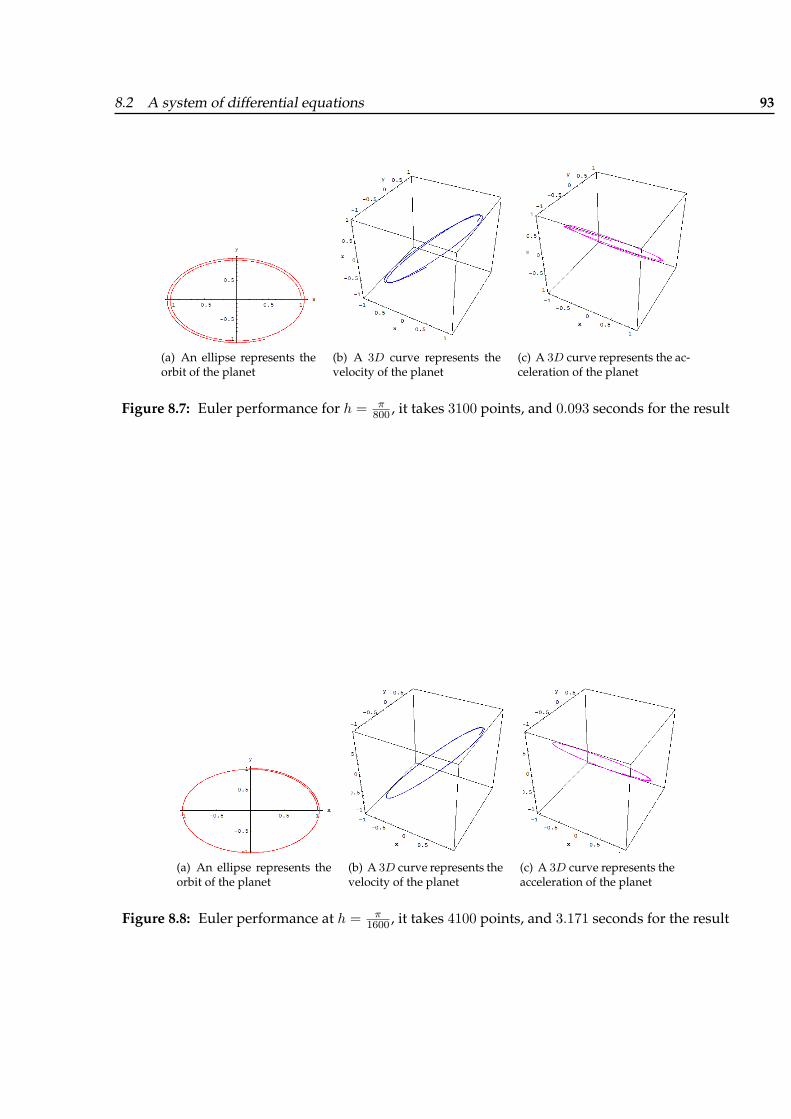
8.2 A system of differential equations 93
(a) An ellipse represents theorbit of the planet
(b) A 3D curve represents thevelocity of the planet
(c) A 3D curve represents the ac-celeration of the planet
Figure 8.7: Euler performance for h = π800 , it takes 3100 points, and 0.093 seconds for the result
(a) An ellipse represents theorbit of the planet
(b) A 3D curve represents thevelocity of the planet
(c) A 3D curve represents theacceleration of the planet
Figure 8.8: Euler performance at h = π1600 , it takes 4100 points, and 3.171 seconds for the result

94 8 Numerical Approach
(a) An ellipse represents theorbit of the planet
(b) A 3D curve representsthe velocity of the planet
(c) A 3D curve representsthe acceleration of theplanet
Figure 8.9: Euler performance for h = π3200 , it takes 8100 points, and 15.813 seconds for the result
(a) An ellipse represents theorbit of the planet
(b) A 3D curve representsthe velocity of the planet
(c) A 3D curve representsthe acceleration of theplanet
Figure 8.10: Euler performance for h = π6400 , it takes 14, 000 points, and 49.032 seconds for the
result
= Second:Heun Heun’s method has two versions, a.k.a modified Euler, or Runge-Kutta secondorder
k1 = hf(xn, yn)
k2 = hf(xn + 12h, yn + 1
2k1)
yn+1 = yn + k2 +O(h3)
(8.19)
which use the midpoint method, i.e. take a “trial” step to the midpoint of the interval. Then use

8.2 A system of differential equations 95
the value of both x and y at that midpoint to compute the “real” step across the whole interval.(See Fig. 8.11)
Figure 8.11: Second Order accuracy is obtained by using the initial derivative at each step to finda point halfway across the interval, then using the midpoint derivative across the full width ofthe interval. In the figure solid dots represent final function values, while open dots representfunction values that are discarded once their derivatives have been calculated and used.
The other form is:
k1 = hf(xn, yn)
k2 = hf(xn + 23h, yn + 2
3k1)
yn+1 = yn + 14k1 + 3
4k2
(8.20)
Both versions have the Truncation Error of O(h2). They have two evaluations per step as younotice, while Euler has but one, accordingly they deliver rather satisfactory results!

96 8 Numerical Approach
(a) An ellipse represents the or-bit of the planet
(b) A 3D curve represents thevelocity of the planet
(c) A 3D curve represents theacceleration of the planet
Figure 8.12: Heun performance for h = π800 , it takes 3100 points, and 2.219 seconds for the result
(a) An ellipse represents the or-bit of the planet
(b) A 3D curve represents thevelocity of the planet
(c) A 3D curve represents the ac-celeration of the planet
Figure 8.13: Heun performance for h = π1600 , it takes 4100 points, and 4.265 seconds for the result

8.2 A system of differential equations 97
(a) An ellipse represents the or-bit of the planet
(b) A 3D curve represents thevelocity of the planet
(c) A 3D curve represents theacceleration of the planet
Figure 8.14: Heun performance for h = π3200 , it takes 8100 points, and 15.343 seconds for the result
= Third:Runge-Kutta Runge-Kutta methods requires four evaluation per a step h.
See Fig. 8.15 for the graphical interpretation.
k1 = hf(xn, yn)
k2 = hf(xn + 12h, yn + 1
2k1)
k3 = hf(xn + 12h, yn + 1
2k2)
k4 = hf(xn + h, yn + k1)
yn+1 = yn + 16(k1 + 2k2 + 2k3 + k4) +O(h5)
(8.21)
An excellent discussion of the pitfalls in constructing a good Runge-Kutta algorithm is given in(17) and (? ).

98 8 Numerical Approach
Figure 8.15: Fourth-order Runge-Kutta method. In each derivative is evaluated four times: onceat the initial point, twice at trial midpoints, and once at a trial endpoint. From these derivativesthe final function value(shown as a filled dot) is calculated.
It has a truncation error of O(h4) then. Butcher (16) has established the relationship between thenumber of evaluations per step and the local truncation error shown in Table.
Evaluations per Step 2 3 4 5 ≤ n ≤ 7 8 ≤ n ≤ 9 10 ≤ n
Best PossibleLocal Truncation Error O(h2) O(h3) O(h4) O(hn−1) O(hn−2) O(hn−3)
Table 8.1: The relation between evaluations number and local truncation error
While for many scientific users, fourth order Runge-Kutta is the α and ω, especially if you combineit with an adaptive step size, but keep in mind Runge-Kutta is just a field-horse and no race-horse, soit’s not the best option though, once speed and high accuracy are required.
The Predictor-corrector methods or Bulirsch-Stoer method proved to be very much more efficient forproblems where very high accuracy is a requirement. These methods are Arabians, real high-strungracehorses. So use Runge-Kutta whenever:
d you don’t know any better, or
d you have an intransigent problem where Predictor-Corrector is falling, or
d you have a trivial problem where computational efficiency is of no concern.

8.2 A system of differential equations 99
(a) An ellipse represents the or-bit of the planet
(b) A 3D curve represents thevelocity of the planet
(c) A 3D curve represents theacceleration of the planet
Figure 8.16: Runge-Kutta performance for h = π800 , it takes 3100 points, and 3.172 seconds for the
result
This will be superior to the midpoint methods Heun and Modified Euler, if at least twice as large astep is possible withRK4 for the same accuracy, and more accurate than Euler with one-quarter ofthe step size h. Is that so? The answer is: often, perhaps even usually, but surely not always. Thismeans that high order does not always imply high accuracy, however for sure it is superior to bothEuler and Heun in a sense of practice of science rather than as a statement of strict mathematics.
Adaptive Step Size A good ODE integrator should exert some adaptive control over its ownProgress, making frequent changes in its step size. Usually the purpose of this step size controlis to achieve some predetermined accuracy Tolerance through estimated truncation error in the solu-tion with minimum computational efforts. Many small steps should tiptoe through treacherousterrain, while a few great strides should speed through smooth uninteresting countryside. Theresulting gain in efficiency can sometimes be factors of ten, a hundred, or more, depends on theproblem in hand.
= Fourth:Runge-Kutta-Fehlberg RKF45 This technique consists of using a Runge-Kuttamethod with local truncation error of order five
yn+1 = yn +16135
k1 +665612825
k3 +2856156430
k4 −95k5 +
255k6,
to estimate the local error in a Runge-Kutta method of order four,
yn+1 = yn +25216
k1 +14082565
k3 +21974104
k4 −15k5,

100 8 Numerical Approach
where
k1 = h f(xn, yn),
k2 = h f(xn +14h, yn +
14k1),
k3 = h f(xn +38h, yn +
332k1 +
932k2),
k4 = h f(xn +1213h, yn +
19322197
k1 −72002179
k2 +72962179
k3),
k5 = h f(xn + h, yn +439216
k1 − 8k2 +3680513
k3 −8454104
k4),
k6 = h f(xn +12h, yn −
827k1 + 2k2 −
35442565
k3 +18594104
k4 −11240
k5),
Error Estimate |yn+1 − yn+1|
Step size qualifier q =(
Tol h
2|yn+1 − yn+1|
)1/4
0 ≤ hmin ≤ h ≤ hmax
(a) An ellipse represents the or-bit of the planet
(b) A 3D curve represents thevelocity of the planet
(c) A 3D curve represents the ac-celeration of the planet
Figure 8.17: Adaptive step size Runge-Kutta-Fehlberg performance for h = π800 , and Tol = 10−13
it takes 3100 points, and 2.203 seconds for the result
See (17) chapter 5 for details. An advantage of this method is that only six evaluations of f arerequired per step. Arbitrary Runge-Kutta methods of order four and five used together require (seeTable 8.1) at least four evaluations of f for the fourth-order method an an additional six for thefifth-order method for a total of at least ten functional evaluations. The value of q is determinedat the nth step for two purposes:
¬ To reject, if necessary, the initial choice of h at the nth step and repeat the calculation using

8.2 A system of differential equations 101
h = q h, and
To predict an appropriate choice of h for the (n+ 1)st step.
Finally it has the local truncation error O(h6).
8 Multi Steps Methods All the previous methods use the information from one previous pointto compute the successive point; that is, only the initial point (x0, y0) is used to compute (x1, y1)and in general, yn is used to compute yn+1. After several points have been found, it is feasi-ble to use several prior points in the calculation. These methods are not self-starting; four ini-tial points (x0, y0), (x1, y1), (x2, y2) and (x3, y3) must be given in advance in order to generate thepoints (xn, yn) : n ≥ 4.
A desirable feature of a multi-step method is that the local truncation error can be determined and acorrection term can be included, which improve the accuracy of the answer at each step. Also, it ispossible to determine if the step size small enough to obtain an accurate value for yn+1, yet largeenough so that unnecessary and time-consuming calculations are eliminated, or even introducean adaptive step size, to increase the speed of the calculations considerably.
Using the combinations of predictor, an explicit method and corrector, an implicit method requires onlytwo function evaluations of f(x, y) per step. Besides boosts the power of the algorithm, to copewith the stiff-equations, because the implicit methods can handle this issue fairly enough.
= Fifth: Adams-Bashforth-Moulton The Adams-Bashforth-Moulton method is a multi-stepmethod derived from the fundamental theorem of calculus:
yn+1 = yn +∫ xn+1
xn
f(x, y(x))dx (8.22)
(a) The four nodes for the Adams-Bashforthpredictor (extrapolation is used)
(b) The four nodes for the Adams-Moultoncorrector (interpolation is used)
Figure 8.18: Integration over [xn, xn+1] in Adams-Bashforth method.

102 8 Numerical Approach
The predictor uses the Lagrange polynomial approximation for f(x, y(x)) based on the points(xn−3, yn−3), (xn−2, yn−2), (xn−1, yn−1) and (xn, yn). It is integrated over the interval [xn, xn+1] in(8.22). This process produces the Adams-Bashforth Explicit Predictor:
pn+1 = yn +h
24(−9fn−3 + 37fn−2 − 59fn−1 + 55fn) (8.23)
The corrector is developed similarly. The value pn+1 just computed can now be used. A sec-ond Lagrange polynomial for f(x, y(x)) is constructed, which is based on the points (xn−2, yn−2),(xn−1, yn−1), (xn, yn), and the new point (xn+1, fn+1) = (xn+1, f(xn+1, pn+1)). This polynomial isthen integrated over [xn, xn+1] producing the Adams-Moulton Implicit Corrector
yn+1 = yn +h
24(fn−2 − 5fn−1 + 19fn + 9fn+1) (8.24)
Fig. 8.18 shows the nodes for the Lagrange polynomials that are used in developing formulas(8.24) and (8.23), respectively.
According to Mathews (18) and Burden (17) the local truncation error error for both the predictorand corrector is of the order O(h5)
τn+1(h) =251720
y(5)(µn)h5 µn ∈ (xn−3, xn+1) (L.T.E for the predictor)
τn+1(h) = − 19720
y(5)(µn)h5 µn ∈ (xn−2, xn+1) (L.T.E for the corrector)

8.2 A system of differential equations 103
(a) An ellipse represents the orbitof the planet
(b) A 3D curve represents the ve-locity of the planet
(c) A 3D curve represents the ac-celeration of the planet
Figure 8.19: Adams-Bashforth-Moulton performance for h = π800 , it takes 1800 points, and 1.281
seconds for the result
= Sixth: Milne-Simpson Another popular Predictor-Corrector scheme. Its predictor is based onintegration of f(x, y(x)) over the interval [xn−3, xn+1].
yn+1 = yn−3 +∫ xn+1
xn−3
f(x, y(x))dx (8.25)
The predictor uses the Lagrange polynomial approximation for f(x, y(x)) based on the points(xn−3, fn−3), (xn−2, fn−2), (xn−1, fn−1) and (xn, fn) over the interval [xn−3, xn+1]. This producesthe Milne Explicit Predictor
pn+1 = yn−3 +4h3
(2fn−2 − fn−1 + 2fn) (8.26)
The value pn+1 can be used to derive the corrector, another Lagrange polynomial which based onthe points (xn−1, fn−1), (xn, fn), and the new point (xn+1, fn+1) = (xn+1, f(xn+1, pn+1)) is con-structed, and the integration is taken over [xn−1, xn+1], the results is the familiar Simpson ImplicitCorrector
yn+1 = yn−1 +h
3(2fn−1 − 4fn + fn+1) (8.27)

104 8 Numerical Approach
(a) An ellipse represents the orbitof the planet
(b) A 3D curve represents the ve-locity of the planet
(c) A 3D curve represents the ac-celeration of the planet
Figure 8.20: Milne-Simpson performance for h = π800 , it takes 1800 points, and 1.265 seconds for
the result
According to Mathews (18) and Burden (17) also the local truncation error error for both the pre-dictor and corrector is of the order O(h5)
τn+1(h) =2890y(5)(µn)h5 µn ∈ (xn−3, xn+1) (L.T.E for the predictor)
τn+1(h) = − 190y(5)(µn)h5 µn ∈ (xn−2, xn+1) (L.T.E for the corrector)
This method, however in practice has less stability than the former one!
= Seventh: Hamming Almost has same performance as Adams-Bashforth-Moulton in this exam-ple it has been even 1.34418 times faster, these two horses are running neck-and-neck in mostapplication.
The Hamming Explicit Predictor over the interval [xn−3, xn+1] :
pn+1 = yn−3 +4h3
(2fn−2 − fn−1 + 2fn) (8.28)
and
The Hamming Implicit Corrector over the interval [xn−2, xn+1] :
yn+1 =yn−2 + 9yn
8+
3h8
(−fn−1 + 2fn + 2fn+1) (8.29)
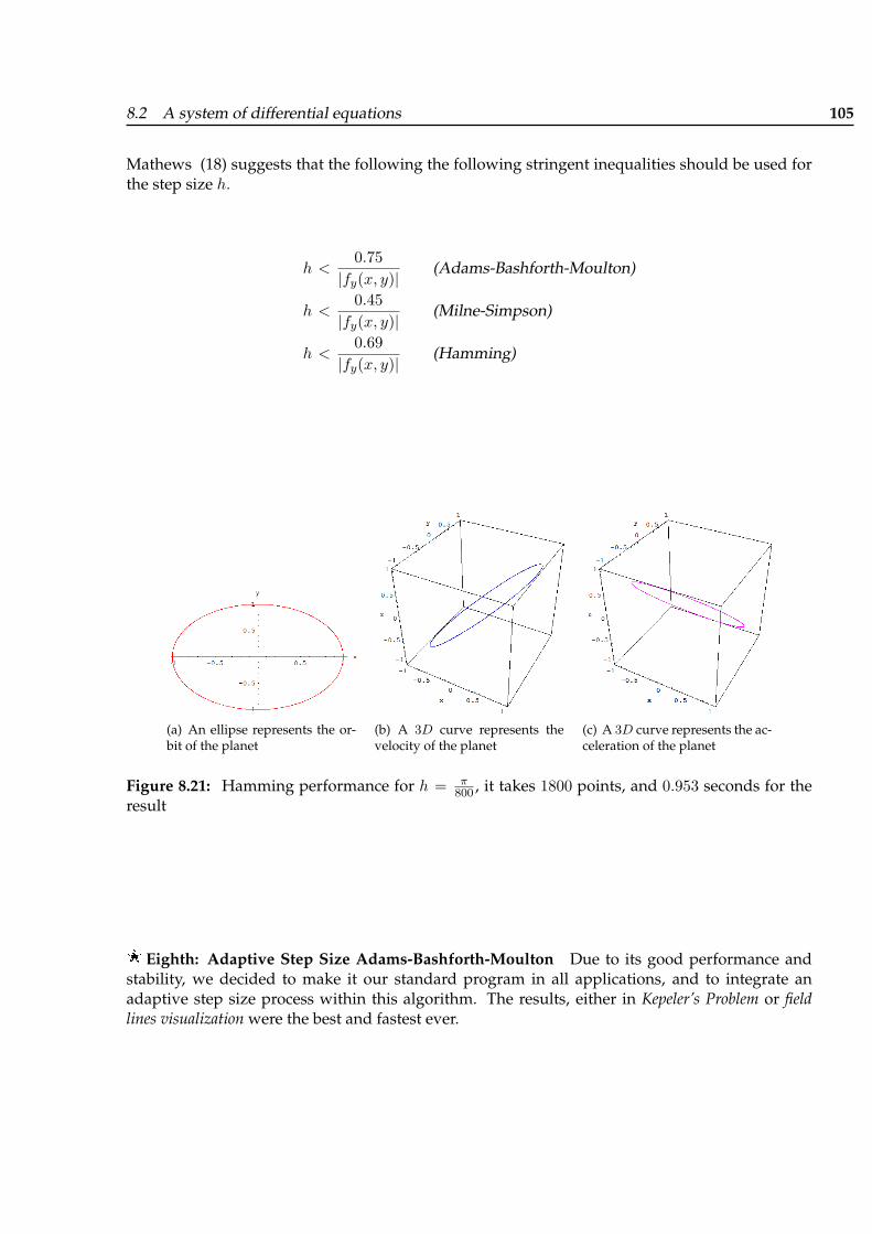
8.2 A system of differential equations 105
Mathews (18) suggests that the following the following stringent inequalities should be used forthe step size h.
h <0.75
|fy(x, y)|(Adams-Bashforth-Moulton)
h <0.45
|fy(x, y)|(Milne-Simpson)
h <0.69
|fy(x, y)|(Hamming)
(a) An ellipse represents the or-bit of the planet
(b) A 3D curve represents thevelocity of the planet
(c) A 3D curve represents the ac-celeration of the planet
Figure 8.21: Hamming performance for h = π800 , it takes 1800 points, and 0.953 seconds for the
result
= Eighth: Adaptive Step Size Adams-Bashforth-Moulton Due to its good performance andstability, we decided to make it our standard program in all applications, and to integrate anadaptive step size process within this algorithm. The results, either in Kepeler’s Problem or fieldlines visualization were the best and fastest ever.

106 8 Numerical Approach
(a) An ellipse represents the or-bit of the planet
(b) A 3D curve represents the veloc-ity of the planet
(c) A 3D curve represents the accel-eration of the planet
Figure 8.22: Adaptive Step Size Adams-Bashforth-Moulton performance for h = π800 , and Tol =
10−13 it takes 1000 points, and 0.609 seconds for the result

107
Chapter 9
Results
Fields of a half-wave dipole can be computed almost as fast as those of the Hertzian dipole (15),whereby the former is of greater relevance. So in the following presentation is made used of thistype of dipole only.
(a) The magnetic field lines of a smallcircular loop antenna, and its mag-netic plane of symmetry
(b) The electric field lines of z-oriented λ
2antenna, and its electric
plane of symmetry
Figure 9.1: Field lines and their corresponding planes of symmetry
9.1 An omnidirectional radiation
The first example considers a single radiator, located at the origin, both linear λ/2 dipole andcircular small loop antenna are present, the figures 9.1 through 9.5. Fig. 9.1 establishes the parallel

108 9 Results
attitude of the magnetic field lines of a loop antenna Fig. 9.1(a) and the electric field lines of alinear antenna Fig. 9.1(b), as well as their magnetic and electric surfaces of symmetry, they bothform the familiar kidney-shaped closed loops.
(a) The electric field lines of a smallcircular loop antenna, and its electricplane of symmetry
(b) The magnetic field lines of z-oriented λ
2antenna, and its magnetic
plane of symmetry
Figure 9.2: Field lines and their corresponding planes of symmetry
(a) The magnetic field lines of asmall circular loop antenna
(b) The electric field lines of z-oriented λ
2antenna, and its mag-
netic plane of symmetry
Figure 9.3: Different circulation of inner and outer formations.
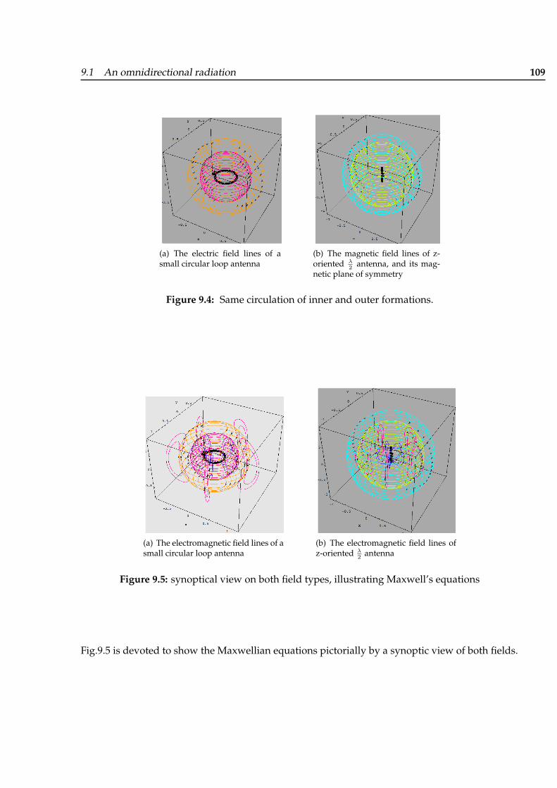
9.1 An omnidirectional radiation 109
(a) The electric field lines of asmall circular loop antenna
(b) The magnetic field lines of z-oriented λ
2antenna, and its mag-
netic plane of symmetry
Figure 9.4: Same circulation of inner and outer formations.
(a) The electromagnetic field lines of asmall circular loop antenna
(b) The electromagnetic field lines ofz-oriented λ
2antenna
Figure 9.5: synoptical view on both field types, illustrating Maxwell’s equations
Fig.9.5 is devoted to show the Maxwellian equations pictorially by a synoptic view of both fields.

110 9 Results
9.2 A directional radiation
Once more than one radiator is involved, the effects of directivity appears clearly in a way thatold omnidirectional fashion of radiation is no longer valid. Omnidirectional antennas have aradiation pattern that is donut shaped with the antenna at the center of the donut. This meansthat with the antenna oriented vertically, the signal coverage is equal in all directions in thehorizontal plane.Directional antennas have a radiation pattern that is more focused than omnidirectional antennas.The coverage area is limited to a conical area of various widths depending on the type ofdirectional antenna. Fig.9.6 is of great relevance, once we decide for a scheme to plot the fieldlines, where they are so dense, and discard them otherwise.
(a) Two-element end-fire (b) four-element end-fire
(c) five-element end-fire (d) six-elementbroadside
Figure 9.6: 3-D Radiation patterns of arrays

9.2 A directional radiation 111
The first example considers two elements, a quarter wavelength apart from each other, and fed asan endfire array. They develop low directivity only, as shown in Fig.9.6(a), the three dimensionalradiation pattern. The formation of its electric and magnetic field lines is given in Fig.9.7(a),Fig.9.7(b) respectively, to improve the visibility in Fig.9.7(a), only one half of the surface ofsymmetry is shown.
(a) The electric field lines of two-element end-fire array
(b) The magnetic field lines of two-element end-fire array
Figure 9.7: The directivity of arrays: two elements
In the second example a four-element endfire array is shown, which may be compared witha short Yagi-Uda-Antenna or the active region of a medium sized logarithmic periodic dipoleantenna (LPD). The pattern shows higher directivity (see Fig.9.6(b), Fig.9.8(a) and Fig.9.8(b) ).The BC, the current lines and the displacement (field) lines in Fig.9.8 are restricted to the mainbeam. In the moment of the snapshot the inner members of the vertical families have alreadydetached from the first dipole, whereas detachment for the outer members has not yet taken place.

112 9 Results
(a) The electric field lines of four-element endfire array
(b) The magnetic field linesof four-element endfire ar-ray
Figure 9.8: The directivity of arrays: four elements
The Figures 9.6(d) and 9.9 consider the electric field launched by a six- element broadside array.In 9.9 two lines families are heading in each main lobe, and one into each side-lobe.
Figure 9.9: The directivity of arrays: six-element broadside array 3D fashion
9.2.1 A passage to 4D visualization
The pattern of the four element array in Fig.9.6(b) reveals a null backwards. Therefore a subdi-vision of the BC, which leads to displacement current lines starting from the negative x-axis, is

9.2 A directional radiation 113
to be avoided. This would represent an almost vanishing portion of the displacement current,Fig.9.8(a).
The next example shall demonstrate that lines can be traced over a given time interval. Thereforea coverage of the full range from the positive to the negative x-axis is necessary. A five-elementendfire array with a medium back-lobe in Fig.9.6(c) allows this coverage and lines can be startedfrom the negative x-axis. In Fig.9.10(b) the inner BC is calculated for a certain moment, the outerfor an eighth of a period later. The displacement currents in Fig.9.10(a) of both moments are shown(magenta color for the later moment) synoptically, this is an application of the 4D visualization,i.e., the spatial and time dependency.
(a) Displacement lines of a five-element endfire array attwo moments with a time difference of 45 degrees
(b) Two boundary contours for two differenttimes of a five-element endfire array
Figure 9.10: The Visualization of the field lines in 4D fashion


115
Appendix
A On small square loop Antenna
The field of an electrically small loop antenna are dependent of the area of loop, but are independentof its shape. In Fig. 11, a model of xy square antenna centered at the origin. The area of the loop isassumed to be (∆`)2 and it carries a uniform current I0.
Figure 11: A small square loop Antenna
The loop may be viewed as four segments, which each represents a Hertzian dipole, each parallelpair carries opposite directed current. Due to the tiny dimensions of that loop, relative to a point

116 Appendix
P in space, the distance vectors from the centers of the four segments become almost parallel, andcan be expressed as
R1 ' r +∆`2
sinϑ sinϕ
R2 ' r − ∆`2
sinϑ cosϕ
(1)
R3 ' r − ∆`2
sinϑ sinϕ
R4 ' r +∆`2
sinϑ cosϕ
The individual magnetic vector potential contributions due to the four segments of the currentloop are given by
~A1 =µ0I0∆`
4πe−β(r+∆`
2sin ϑ sin ϕ)
r + ∆`2 sinϑ sinϕ
~ex
~A2 =µ0I0∆`
4πe−β(r−∆`
2sin ϑ cos ϕ)
r − ∆`2 sinϑ cosϕ
~ey
(2)
~A3 =µ0I0∆`
4πe−β(r−∆`
2sin ϑ sin ϕ)
r − ∆`2 sinϑ sinϕ
(−~ex)
~A4 =µ0I0∆`
4πe−β(r+∆`
2sin ϑ cos ϕ)
r + ∆`2 sinϑ cosϕ
(−~ey)
We need to define another four functions, which can be expressed in a Maclaurin series about ∆`,these functions are:

A On small square loop Antenna 117
f1 =e−β(r+∆`
2sin ϑ sin ϕ)
r + ∆`2 sinϑ sinϕ
f2 =e−β(r−∆`
2sin ϑ cos ϕ)
r − ∆`2 sinϑ cosϕ
f3 =e−β(r−∆`
2sin ϑ sin ϕ)
r − ∆`2 sinϑ sinϕ
(3)
f4 =e−β(r+∆`
2sin ϑ cos ϕ)
r + ∆`2 sinϑ cosϕ
Using the expression (4), each term can be expanded as in Eq. (5), which are very good approxi-mations by considering just the first two terms of Eq. (4):
f = f(0) + f ′(0)∆`+12f ′′(0)(∆`)2 + . . .
(4)
f ′(0) =∂f
∂∆`
∣∣∣∣∆`=0
, f ′′(0)∂2f
∂∆`2
∣∣∣∣∆`=0
, . . .
f1 =(
1r− ∆`
2
(β
r+
1r2
)sinϑ sinϕ
)e−βr
f2 =(
1r
+∆`2
(β
r+
1r2
)sinϑ cosϕ
)e−βr
f3 =(
1r
+∆`2
(β
r+
1r2
)sinϑ sinϕ
)e−βr (5)
f4 =(
1r− ∆`
2
(β
r+
1r2
)sinϑ cosϕ
)e−βr

118 Appendix
We can now simply combine the x-directed and y-directed terms, which yields:
Ax = | ~A1 + ~A3|
=µ0I0∆`
4π
(1r− ∆`
2
(β
r+
1r2
)sinϑ sinϕ−
1r− ∆`
2
(β
r+
1r2
)sinϑ sinϕ
)e−βr
= −µ0I0(∆`)2
4π
((β
r+
1r2
)sinϑ sinϕ
)e−βr
(6)Ay = | ~A2 + ~A4|
=µ0I0∆`
4π
(1r
+∆`2
(β
r+
1r2
)sinϑ cosϕ−
1r
+∆`2
(β
r+
1r2
)sinϑ cosϕ
)e−βr
=µ0I0(∆`)2
4π
((β
r+
1r2
)sinϑ cosϕ
)e−βr
The terms of Eq. (6) can be expressed in the rectangular coordinates
Ax = −µ0I0(∆`)2
4πe−βr
(β
r+
1r2
)√x2 + y2
r
y
√x2 + y2
= −µ0I0(∆`)2
4πy e−βr
(β
r2+
1r3
)(7)
Ay =µ0I0(∆`)2
4πe−βr
(β
r+
1r2
)√x2 + y2
r
x
√x2 + y2
=µ0I0(∆`)2
4πx e−βr
(β
r2+
1r3
)Az = 0.
The magnetic fields are determined according to Eq. (8)
~H =1µ0∇× ~A = Hx~ex +Hy~ey +Hz~ez (8)
where
∇× ~A =
7
0∂Az
∂y− ∂Ay
∂z
~ex +
∂Ax
∂z−
0
∂Az
∂x
~ey +(∂Ay
∂z− ∂Ax
∂y
)~ez (9)

A On small square loop Antenna 119
Therefore,
Hx = − 1µ0
∂Ay
∂z
= −I0(∆`)2
4πx∂
∂z
((β
r2+
1r3
)e−βr
)
= −I0(∆`)2
4πx
((β
r2+
1r3
)∂e−βr
∂z+ e−βr ∂
∂z
(β
r2+
1r3
))
= −I0(∆`)2
4πx
((β
r2+
1r3
)(−β z
re−βr
)+ e−βr
(β
2 zr4
+3 zr5
))
= −I0(∆`)2
4πx
(β2 z
r3− β
z
r4− β
2 zr4− 3 zr5
)e−βr
= −I0(∆`)2
4πx
(β2 z
r3− β
3 zr4− 3 zr5
)e−βr
=I0(∆`)2
4π
(3 z xr5
+ β3 z xr4
− β2 z x
r3
)e−βr (10)
Hy = − 1µ0
∂Ax
∂z
=I0(∆`)2
4πy∂
∂z
((β
r2+
1r3
)e−βr
)
=I0(∆`)2
4πy
((β
r2+
1r3
)∂e−βr
∂z+ e−βr ∂
∂z
(β
r2+
1r3
))
=I0(∆`)2
4πy
((β
r2+
1r3
)(−β z
re−βr
)+ e−βr
(β
2 zr4
+3 zr5
))
=I0(∆`)2
4πy
(β2 z
r3− β
z
r4− β
2 zr4− 3 zr5
)e−βr
=I0(∆`)2
4πy
(β2 z
r3− β
3 zr4− 3 zr5
)e−βr
= −I0(∆`)2
4π
(3 z yr5
+ β3 z yr4
− β2 z y
r3
)e−βr (11)
and
Hz =1µ0
(∂Ay
∂x− ∂Ax
∂y
)(12)
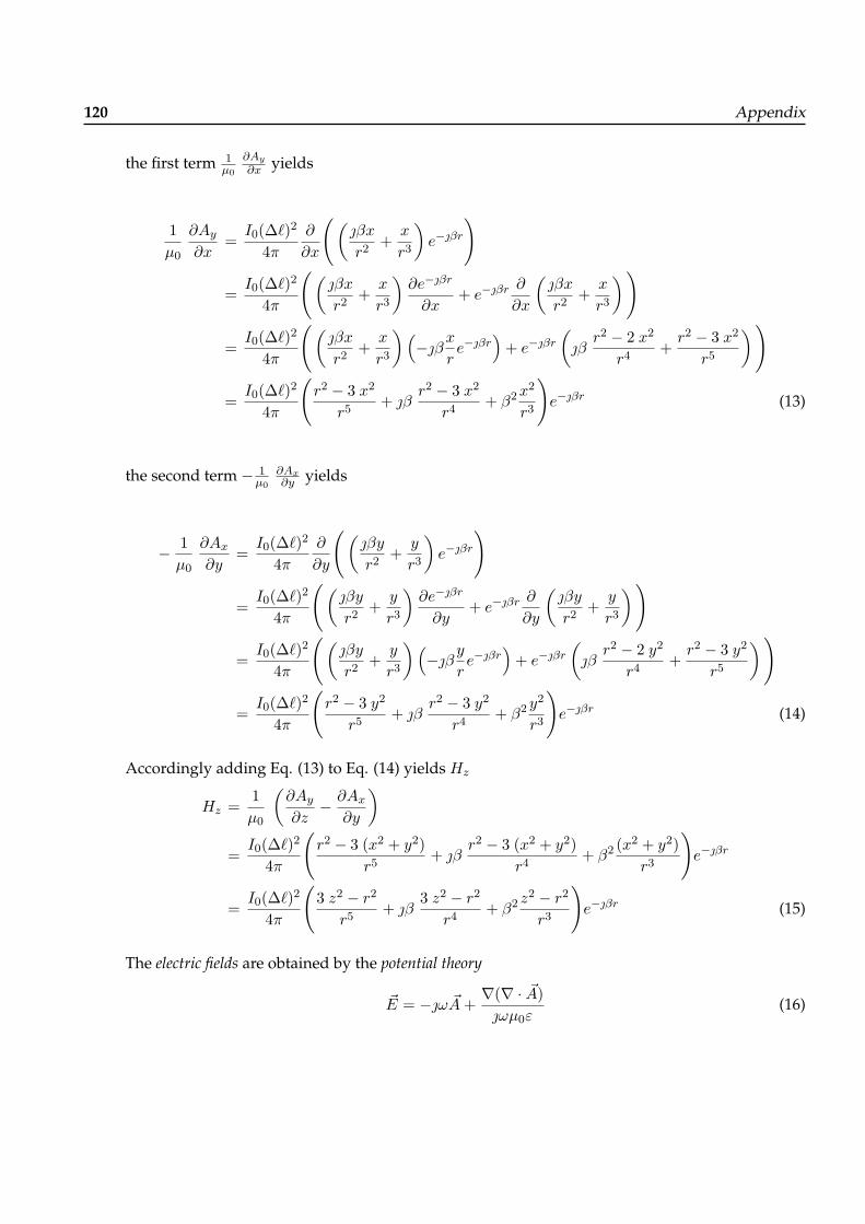
120 Appendix
the first term 1µ0
∂Ay
∂x yields
1µ0
∂Ay
∂x=I0(∆`)2
4π∂
∂x
((βx
r2+x
r3
)e−βr
)
=I0(∆`)2
4π
((βx
r2+x
r3
)∂e−βr
∂x+ e−βr ∂
∂x
(βx
r2+x
r3
))
=I0(∆`)2
4π
((βx
r2+x
r3
)(−β x
re−βr
)+ e−βr
(β
r2 − 2 x2
r4+r2 − 3 x2
r5
))
=I0(∆`)2
4π
(r2 − 3 x2
r5+ β
r2 − 3 x2
r4+ β2x
2
r3
)e−βr (13)
the second term − 1µ0
∂Ax∂y yields
− 1µ0
∂Ax
∂y=I0(∆`)2
4π∂
∂y
((βy
r2+
y
r3
)e−βr
)
=I0(∆`)2
4π
((βy
r2+
y
r3
)∂e−βr
∂y+ e−βr ∂
∂y
(βy
r2+
y
r3
))
=I0(∆`)2
4π
((βy
r2+
y
r3
)(−β y
re−βr
)+ e−βr
(β
r2 − 2 y2
r4+r2 − 3 y2
r5
))
=I0(∆`)2
4π
(r2 − 3 y2
r5+ β
r2 − 3 y2
r4+ β2 y
2
r3
)e−βr (14)
Accordingly adding Eq. (13) to Eq. (14) yields Hz
Hz =1µ0
(∂Ay
∂z− ∂Ax
∂y
)=I0(∆`)2
4π
(r2 − 3 (x2 + y2)
r5+ β
r2 − 3 (x2 + y2)r4
+ β2 (x2 + y2)r3
)e−βr
=I0(∆`)2
4π
(3 z2 − r2
r5+ β
3 z2 − r2
r4+ β2 z
2 − r2
r3
)e−βr (15)
The electric fields are obtained by the potential theory
~E = −ω ~A+∇(∇ · ~A)ωµ0ε
(16)

A On small square loop Antenna 121
Let’s check up whether ∇ · ~A != 0? Where
∇ · ~A =∂Ax
∂x~ex +
∂Ay
∂y~ey +
>
0∂Az
∂z~ez (17)
The first term of Eq. (17) is
∂Ax
∂x= −µ0I0(∆`)2
4πy∂
∂x
((β
r2+
1r3
)e−βr
)
= −µ0I0(∆`)2
4πy
((β
r2+
1r3
)∂e−βr
∂x+ e−βr ∂
∂x
(β
r2+
1r3
))
= −µ0I0(∆`)2
4πy
((β
r2+
1r3
)(−β x
re−βr
)+ e−βr
(β−2 xr4
+−3 xr5
))
=µ0I0(∆`)2
4π
(− 3 x y
r5− β
3 x yr4
+ β2x y
r3
)e−βr (18)
and the second term of Eq. (17) is
∂Ay
∂y=µ0I0(∆`)2
4πx∂
∂y
((β
r2+
1r3
)e−βr
)
=µ0I0(∆`)2
4πx
((β
r2+
1r3
)∂e−βr
∂y+ e−βr ∂
∂y
(β
r2+
1r3
))
=µ0I0(∆`)2
4πx
((β
r2+
1r3
)(−β y
re−βr
)+ e−βr
(β−2 yr4
+−3 yr5
))
=µ0I0(∆`)2
4π
(3 x yr5
+ β3 x yr4
− β2x y
r3
)e−βr (19)
Indeed adding Eq. (18) to Eq. (19) yields that ∇ · ~A = 0.
Eq. (16) is thus reduced to
~E = −ω ~A = −ωAx ~ex − ωAy ~ey
= Ex ~ex + Ey ~ey (20)=⇒

122 Appendix
Ex = − ωAx
= ωµ0I0(∆`)2
4πy
( β
r2+
1r3
)e−βr
= β
√µ0 ε0
µ0I0(∆`)2
4πy
(β
r2+
1r3
)e−βr
= β
õ0
ε0
I0(∆`)2
4πy
(β
r2+
1r3
)e−βr
= β ηI0(∆`)2
4πy
(β
r2+
1r3
)e−βr (21)
and
Ey = − ωAy
= − ωµ0I0(∆`)2
4πx
( β
r2+
1r3
)e−βr
= − β√µ0 ε0
µ0I0(∆`)2
4πx
(β
r2+
1r3
)e−βr
= − β√µ0
ε0
I0(∆`)2
4πx
(β
r2+
1r3
)e−βr
= − β η I0(∆`)2
4πx
(β
r2+
1r3
)e−βr (22)
and finallyEz = 0. (23)

B On small circular loop Antenna
Any antenna used for transmission has the same goal. By generating an alternating current in aconductor, a rapidly changing electrical field is induced in free space. An electrical field cannotexist without a magnetic field component. These fields propagate until reaching another conduc-tor - in which an alternating current similar to the original is induced. The only difference beingthe much lower energy level.
To make the transfer of energy from transmitter to antenna, and from antenna to space mostefficient, the antenna is made resonant - in other words the alternating current flowing withinthe antenna swings to and fro at a rate that matches the arrival of each peak of current from thetransmitter. It’s like pushing a child on a swing - if you push at the same rate that the swing ismoving, you get bigger swings for your effort...
A magnetic loop antenna is so called because unlike a conventional wire dipole the small trans-mitting loop aims to generate the magnetic field rather than the electrical one. The result is thesame once the radio wave is produced. Both the magnetic and electrical components propagate asbefore. The significance of generating a magnetic field lies in the tendency of magnetic fields to becaptured by nearby conductors, but to be less affected by nearby ground. This may be because themagnetic field falls away more rapidly with distance than the electric field. This doesn’t mean thatsmall loops prefer being near the ground - but it does seem to suggest that they may be happierthan the equivalent ’electrical’ antenna at the same hight. Very low dipoles tend to radiate straightup!
Symmetric loop antennas have a plane of symmetry running along the feed and through the loop.Planar loop antennas lie in a single plane which also contains the conductors of the feed.
Three-dimensional loop antennas have wire which runs in all of the x, y, and z directions (in a rect-angular Cartesian system). By definition they are not planar. They may, however, be symmetricabout planes which contain the feed.
In the case of vanishingly small loops, the traditional calculation assumes that the current ele-ment I0 ~d`′ is the same everywhere around the loop perimeter, as can be seen diagrammatically inFig. 12. In this case, the radiation along any loop diameter arrives from an oppositely directed butparallel element of current after a short time delay, which puts in a phase shift so that the radiationcontributions do not entirely cancel.

124 Appendix
Figure 12: A small circular loop Antenna
Even a single, straight wire conductor has an electrical and magnetic field around it so long as thecurrent flowing in it varies over time. However by coiling this conductor, the magnetic lines offorce are concentrated (this is the basis of an electromagnet). Small transmitting loop antennas, aretherefor small (single turn) coil antennas! Multiple turn small transmitting loop (STL) antennashave been successfully built and used.
The resonance of a dipole antenna is determined by its size - the smallest resonant length is ahalf wavelength long (slightly smaller in fact because radio frequency travels more slowly in aconductor than in free space ). It is this ’half-wavelength limitation’ that gives the magnetic loopits sense of appeal, or even dare I say, mystery?
A magnetic loop antenna is comprised of a (usually but not necessarily) round conductor of atotal length perhaps one quarter or more commonly for short wave one fifth or one eight of awavelength. Loops made from conductors longer than a quarter wave-length, probably behavemore like delta loop antennas.
Since frequency multiplied by wavelength always equals the speed of light, the higher the oper-

B On small circular loop Antenna 125
ating frequency, the smaller the half wave antenna can be. This isn’t so small. The magnetic loop,or small transmitting loop (STL) antenna appears to offer some performance without needing thatmystical half-wavelength measurement. Indeed the whole operation of magnetic loops generatesconsiderable debate. The pivot of this argument is the possibility that a small magnetic loop mightbe as effective as a half wave wire antenna. It is surprisingly difficult to establish one way or theother as to whether this is in fact the case.
Unlike the approach used before, in deriving Time-varying expression for a linear Dipole antenna,we will use the phasor notation this time, because it is much simpler. The shape of the antenna isno matter, it could be instead, a rectangular, square, triangle, ellipse or any symmetrical figure, tosimplify the calculations in analysis and construction.
Firstly the Magnetic Vector Potential MPV ~A of a circular loop of radius a Fig. 12, at the observationpoint in space P has to be found, whereR a. Due to the cylindrical symmetry, one deduces that~A is independent of the azimuthal angle ϕ′. The position vectors of P and the integration point Q,which lies in the middle of a current-element I0 ~d`′ are defined as the following:
~r = ~r′ + ~R (24)~r′ = a cosϕ′ ~ex + a sinϕ′ ~ey (25)~r = x~ex + z ~ez taken at ϕ′ = 0 for simplicity (26)
Therefore we have,
~R = ~r′ − ~r′
=√x2 + z2 − 2 a x cosϕ′ + a2
=√r2 − 2 a r sinϑ cosϕ′ + a2
= r
√1− 2
a
rsinϑ cosϕ′ + (
a
r)2
The term(
ar
)2 can be neglected due to the assumption r a, thus we have
R ' r
√1− 2
a
rsinϑ cosϕ′ (27)
Applying the binomial theorem
(a+ b)n = n an−1b+n(n− 1)
2!an−2b2 +
n(n− 1)(n− 2)3!
an−3b3 + . . .
on Eq. (27), further simplification can be obtained:
R ' r
√1− a
rsinϑ cosϕ′ (28)

126 Appendix
The infinitesimal segment of the loop d`′ is defined as d`′ = adϕ′, therefore in a thin wire ~A isgiven by:
~A(x, y, z) =µ0
4π
∫e
~Ic(x′, y′, z′)e−βR
Rd`′ (29)
The current ~Ie(x′, y′, z′) can be expressed in its three cartesian components
~Ie(x′, y′, z′) = Ix(x′, y′, z′)~ex + Iy(x′, y′, z′)~ey + Iz(x′, y′, z′)~ez
The current ~Ie(x′, y′, z′) in Fig. 12 flows in ~eϕ = − sinϕ′~ex + cosϕ′~ey direction, therefore it is
~Ie = −Ix sinϕ′~ex + Iy cosϕ′~ey
Assuming a very thin loop, enables us to assume that Ix = Ix = I0, where I0 is constant, whichyields:
~A =µ0I0a
4π
∫ 2π
0
e−β(r−a sin ϑ cos ϕ′)
(r − a sinϑ cosϕ′)dϕ′~eϕ
= −µ0I0a
4π
∫ 2π
0sinϕ′
e−β(r−a sin ϑ cos ϕ′)
(r − a sinϑ cosϕ′)dϕ′~ex
+µ0I0a
4π
∫ 2π
0cosϕ′
e−β(r−a sin ϑ cos ϕ′)
(r − a sinϑ cosϕ′)dϕ′~ey (30)
For a small loop, the function f = e−β(r−a sin ϑ cos ϕ′)
(r−a sin ϑ cos ϕ′) can be expanded in Maclaurin Series about a = 0using:
f = f(0) + f ′(0)a+12!f ′′(0)a2 + · · ·+ 1
(n− 1)!fn−1an−1 + . . .
where f ′ = ∂f∂a |a=0, f
′′ = ∂2f∂a2 |a=0, . . . , f
m = ∂mf∂am |a=0 . We consider only the first two terms of the
expansion:
f(0) =e−βr
r
f ′(0) = a
(β
r+
1r2
)sinϑ cosϕ′
e−βr
r
f '(
1r
+ a
(β
r+
1r2
)sinϑ cosϕ′
)e−βr
r(31)

B On small circular loop Antenna 127
Using the previous relations in ~A
~A =µ0I0a
4π
∫ 2π
0
(− sinϕ′
e−βr
r
(1r
+ a
(β
r+
1r2
)sinϑ cosϕ′
)dϕ′
+cosϕ′e−βr
r
(1r
+ a
(β
r+
1r2
)sinϑ cosϕ′
)dϕ′
)(32)
and observing that the integration∫ 2π0 sinϕ′ cosϕ′ = 0 the Eq. (32) can be further simplified to
~A = Aϕ~eϕ =µ0I0a
4π
∫ 2π
0cosϕ′
e−βr
r
(1r
+ a
(β
r+
1r2
)sinϑ cosϕ′
)dϕ′
=µ0I0a
4πe−βr
rsinϑ
∫ 2π
0
(1r
+ a
(β
r+
1r2
)cos2 ϕ′
)dϕ′~eϕ
=µ0I0a
4e−βr
r
(1r
+ a
(β
r+
1r2
))sinϑ ~eϕ
' µ0I0a2
4e−βr
r
(β
r+
1r2
)sinϑ ~eϕ (33)
Accordingly we have
Ax = − sinϕAϕ
Ay = cosϕAϕ (34)Az = 0
which can be expressed in the cartesian coordinates x, y, z
Ax = −(a
2
)2µ0I0 e
−βr
(β
r+
1r2
)√x2 + y2
r
y
√x2 + y2
= −(a
2
)2µ0I0 e
−βr y
r
(β
r+
1r2
)(35)
Similarly we obtain
Ay =(a
2
)2µ0I0 e
−βr
(β
r+
1r2
)√x2 + y2
r
x
√x2 + y2
=(a
2
)2µ0I0 e
−βr x
r
(β
r+
1r2
)(36)

128 Appendix
The magnetic field components can now be obtained using the relation:
~H = Hx~ex +Hy~ey +Hz~ez =1µ0∇× ~A (37)
where
∇× ~A =
7
0∂Az
∂y− ∂Ay
∂z
~ex +
∂Ax
∂z−
0
∂Az
∂x
~ey +
(∂Ay
∂x− ∂Ax
∂y
)~ez (38)
B.1 The Magnetic Fields
Hx = − 1µ0
∂Ay
∂z
= −(a
2
)2I0 x
∂
∂z
((β
r2+
1r3
)e−βr
)
= −(a
2
)2I0 x
((β
r2+
1r3
)∂e−βr
∂z+ e−βr ∂
∂z
(β
r2+
1r3
))
= −(a
2
)2I0 x
((β
r2+
1r3
)(−β z
re−βr
)− e−βr
(2 β
z
r4+
3 zr5
))
=(a
2
)2I0
(3 x zr5
+ β3 x zr4
− β2 x z
r3
)e−βr (39)
Hy =1µ0
∂Ax
∂z
= −(a
2
)2I0 y
∂
∂z
((β
r2+
1r3
)e−βr
)
= −(a
2
)2I0 y
((β
r2+
1r3
)∂e−βr
∂z+ e−βr ∂
∂z
(β
r2+
1r3
))
= −(a
2
)2I0 y
((β
r2+
1r3
)(−β z
re−βr
)− e−βr
(2 β
z
r4+
3 zr5
))
=(a
2
)2I0
(3 y zr5
+ β3 y zr4
− β2 y z
r3
)e−βr (40)
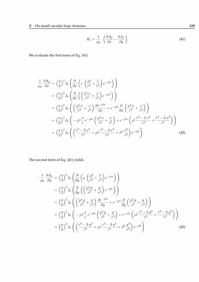
B On small circular loop Antenna 129
Hz =1µ0
(∂Ay
∂x− ∂Ax
∂y
)(41)
We evaluate the first term of Eq. (41)
1µ0
∂Ay
∂x=(a
2
)2I0
(∂
∂x
(x
(β
r2+
1r3
)e−βr
))
=(a
2
)2I0
(∂
∂x
((β x
r2+x
r3
)e−βr
))
=(a
2
)2I0
((β x
r2+x
r3
)∂e−βr
∂x+ e−βr ∂
∂x
(β x
r2+x
r3
))
=(a
2
)2I0
(− β
x
re−βr
(β x
r2+x
r3
)+ e−βr
(β
r2 − 2 x2
r4+r2 − 3 x2
r5
))
=(a
2
)2I0
((r2 − 3 x2
r5+ β
r2 − 3 x2
r4+ β2 x
2
r3
)e−βr
)(42)
The second term of Eq. (41) yields
− 1µ0
∂Ax
∂y=(a
2
)2I0
(∂
∂y
(y
(β
r2+
1r3
)e−βr
))
=(a
2
)2I0
(∂
∂y
((β y
r2+
y
r3
)e−βr
))
=(a
2
)2I0
((β y
r2+
y
r3
)∂e−βr
∂y+ e−βr ∂
∂y
(β y
r2+
y
r3
))
=(a
2
)2I0
(− β
x
re−βr
(β y
r2+
y
r3
)+ e−βr
(β
r2 − 2 y2
r4+r2 − 3 y2
r5
))
=(a
2
)2I0
((r2 − 3 y2
r5+ β
r2 − 3 y2
r4+ β2 y
2
r3
)e−βr
)(43)

130 Appendix
Adding (42) to (43) results in Hz
Hz =1µ0
(∂Ay
∂x− ∂Ax
∂y
)=(a
2
)2I0
(r2 − 3 x2 + r2 − 3 y2
r5+ β
r2 − 3 x2 + r2 − 3 y2
r4+ β2 x
2 + y2
r3
)e−βr
=(a
2
)2I0
(2 r2 − 3 (x2 + y2)
r5+ β
2 r2 − 3 (x2 + y2)r4
+ β2 x2 + y2
r3
)e−βr
=(a
2
)2I0
(3 z2 − r2
r5+ β
3 z2 − r2
r4+ β2 z
2 − r2
r3
)e−βr (44)
This time we will use the potential theory ~E = −ω ~A − ∇ϕ, to derive the electric fields expressions,where according to Lorentz Gauge ϕ = − 1
ωµ0ε0∇(∇ · ~A), thus we have
~E = −ω ~A+1
ωµ0ε0∇(∇ · ~A) (45)
Let’s examine whether the second term of Eq. (45) yields a zero?
∇ · ~A =∂Ax
∂x+∂Ay
∂y+
0
∂Az
∂z=⇒∂Ax
∂x= −
(a2
)2µ0I0 y
((βr
r2+
1r3
)∂e−βr
∂x+ e−βr ∂
∂x
(β
r2+
1r3
))
= −(a
2
)2µ0I0 y
((β
r2+
1r3
)(−β x
re−βr
)+ e−βr
(−β 2 x
r4− 3 x
r5
))
= −(a
2
)2µ0I0
(β2x y
r3− β
3 x yr4
− 3 x yr5
)e−βr
=(a
2
)2µ0I0
(− β2x y
r3+ β
3 x yr4
+3 x yr5
)e−βr

B On small circular loop Antenna 131
and
∂Ay
∂y=(a
2
)2µ0I0 x
((βr
r2+
1r3
)∂e−βr
∂y+ e−βr ∂
∂y
(β
r2+
1r3
))
=(a
2
)2µ0I0 x
((β
r2+
1r3
)(−β y
re−βr
)+ e−βr
(−β 2 y
r4− 3 yr5
))
=(a
2
)2µ0I0
(β2x y
r3− β
3 x yr4
− 3 x yr5
)e−βr
=⇒
∂Ax
∂x+∂Ay
∂y= ∇ · ~A = 0. (46)
The electric fields can be now easily obtained
B.2 The Electric Fields
~E = −ω ~A = −ω Ax~ex − ω Ay~ey = Ex~ex + Ey~ey (47)
All we need is to substitute for Eq. (35) and Eq. (36) in their counterparts in Eq. (47) to get theresults:
Ex = −ω Ax
= ω(a
2
)2µ0I0 y
(β y
r2+
y
r3
)e−βr
= µ0ω(a
2
)2I0 y
(β y
r2+
y
r3
)e−βr
= µ0β
√µ0ε0
(a2
)2I0 y
(β y
r2+
y
r3
)e−βr
= β
õ0
ε0
(a2
)2I0 y
(β y
r2+
y
r3
)e−βr (48)

132 Appendix
Ey = −ω Ay
= −ω(a
2
)2µ0I0 x
(β x
r2+x
r3
)e−βr
= −µ0ω(a
2
)2I0 x
(β x
r2+
x
r3
)e−βr
= −µ0β
√µ0ε0
(a2
)2I0 x
(β x
r2+
x
r3
)e−βr
= −β√µ0
ε0
(a2
)2I0 x
(β x
r2+
x
r3
)e−βr (49)
and
Ez = −ω >
0Az = 0. (50)
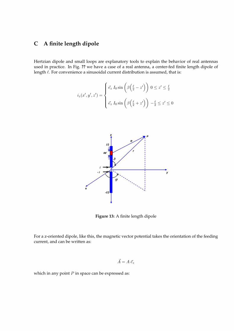
C A finite length dipole
Hertzian dipole and small loops are explanatory tools to explain the behavior of real antennasused in practice. In Fig. ?? we have a case of a real antenna, a center-fed finite length dipole oflength `. For convenience a sinusoidal current distribution is assumed, that is:
iz(x′, y′, z′) =
~ez I0 sin
(β(
`2 − z′
))0 ≤ z′ ≤ `
2
~ez I0 sin(β(
`2 + z′
))− `
2 ≤ z′ ≤ 0
Figure 13: A finite length dipole
For a z-oriented dipole, like this, the magnetic vector potential takes the orientation of the feedingcurrent, and can be written as:
~A = A ~ez
which in any point P in space can be expressed as:

134 Appendix
~A =µ I04π
∫ 0
− `2
sin(β( `
2− z′
))e−βR
Rdz′
+ sin(β( `
2+ z′
))e−βR
Rdz′~ez (51)
Assuming a very thing wire, implies further simplifications, that is x′ = y′ = 0, and from anypoint on the dipole to a space point P , the distance R can be expressed as:
R =√
(x− x′)2 + (y − y′)2 + (z − z′)2
=√
(x)2 + (y)2 + (z − z′)2 (52)
From Maxwell’s equations we know that
∇ · ~B = 0 =⇒ ~B = ∇× ~A
therefore, in free space we have
~B = µ0~H
~H =1µ0∇× ~A (53)
=⇒
∇× ~A =
∂Az
∂y−
0
∂Ay
∂z
~ex +
0∂Ax
∂z− ∂Az
∂x
~ey +
*0
∂Ay
∂x− ∂Ax
∂y
~ez=∂Az
∂y~ex +
∂Az
∂x~ey (54)
Accordingly equation (53) can be expressed as
~H =1µ0
∂Az
∂y~ex +
1µ0
∂Az
∂x~ey = Hx ~ex +Hy ~ey (55)
Using Euler’s Identity
sin(β( `
2± z′
))=eβ( `
2±z′) + e−β( `
2±z′)
2
and (51) in (53), the x-component of the magnetic field yields:

C A finite length dipole 135
Hx =I04π
∂
∂y
(∫ 0
−`/2
(eβ( `2+z′) − e−β( `
2+z′))
2e−βR
Rdz′
+∫ `/2
0
(eβ( `2−z′) − e−β( `
2−z′))
2e−βR
Rdz′)
=I08π
eβ`/2
∫ 0
−`/2
∂
∂y
(e−jβ(R−z′)
R
)dz′
−e−β`/2
∫ 0
−`/2
∂
∂y
(e−jβ(R+z′)
R
)dz′
+eβ`/2
∫ `/2
0
∂
∂y
(e−jβ(R+z′)
R
)dz′
−e−β`/2
∫ `/2
0
∂
∂y
(e−jβ(R−z′)
R
)dz′
(56)
Now we examine the terms in (56) closely, the term eβ`/2∫ `/20
∂∂y
(e−jβ(R+z′)
R
)dz′ for instance can
be rearranged as:
eβ`/2
∫ `/2
0
∂
∂y
(e−jβ(R+z′)
R
)dz′ = eβ`/2
∫ `/2
0
1R
∂
∂y
(e−jβ(R+z′)
)+ e−jβ(R+z′) ∂
∂y
(1R
)= y eβ`/2
∫ `/2
0
(− β
e−jβ(R+z′)
R2− e−jβ(R+z′)
R3
)dz′ (57)
The term in (57) can considerably simplified if we tailored a suitable differentiation that exactlymatches it, therefore consider the the following differentiation:
∂
∂z′
(e−jβ(R+z′)
R(R+ z′ − z)
)=
∂
∂z′
(R−1(R+ z′ − z)−1e−jβ(R+z′)
)= e−jβ(R+z′)
(1
(R+ z′ − z)∂R−1
∂z′+
1R
∂
∂z′(R+ z′ − z)−1
−β ∂
∂z′(R+ z′)
R(R+ z′ − z)
)(58)

136 Appendix
The first term in (58) yields:
1(R+ z′ − z)
∂R−1
∂z′=(
z − z′
R3(R+ z′ − z)
)(59)
The second term in (58) yields:
1R
∂
∂z′(R+ z′ − z)−1 = −
(1R2
1(R+ z′ − z)
)(60)
and eventually the third term yields:
− β
R(R+ z′ − z)∂
∂z′(R+ z′) = −β
(1R2
)(61)
Therefore their sum yields:
∂
∂z′
(e−jβ(R+z′)
R(R+ z′ − z)
)= e−jβ(R+z′)
(z − z′
R3(R+ z′ − z)
− 1R2(R+ z′ − z)
− β
(1R2
))
= e−jβ(R+z′)
(− 1R3
− β1R2
)(62)
We, thus can use (62) in (57) and get:

C A finite length dipole 137
eβ`/2
∫ `/2
0
∂
∂y
(e−jβ(R+z′)
R
)dz′ = y eβ`/2
∫ `/2
0
(− β
e−jβ(R+z′)
R2− e−jβ(R+z′)
R3
)dz′
= y eβ`/2
∫ `/2
0
(− β
e−jβ(R+z′)
R2− e−jβ(R+z′)
R3
)dz′
= y eβ`/2
∫ `/2
0
∂
∂z′
(e−jβ(R+z′)
R(R+ z′ − z)
)dz′
= y eβ`/2
[e−jβ(R+z′)
R(R+ z′ − z)
∣∣∣∣∣`/2
0
(63)
For further simplifications, of (62) we introduce two more dimensionsR1 andR2, which representeach the distance between the space point P and the upper and lower tips of the dipole, as shownin Fig. 14, these are defined as:
R1 =
√x2 + y2 + (z − `
2)2
R2 =
√x2 + y2 + (z +
`
2)2
Figure 14: A finite length dipole
Using (52), R1 and R2 in (63) we get:

138 Appendix
eβ`/2
∫ `/2
0
∂
∂y
(e−jβ(R+z′)
R
)dz′ = y eβ`/2
(e−jβ(R+z′)
R1(R1 + `2 − z)
− e−jβr
r(r − z)
)(64)
In a similar manner, eβ`/2∫ 0−`/2
∂∂y
(e−jβ(R−z′)
R
)dz′ can also be computed:
eβ`/2
∫ 0
−`/2
∂
∂y
(e−jβ(R−z′)
R
)dz′ = eβ`/2
∫ 0
−`/2
1R
∂
∂y
(e−jβ(R−z′)
)+ e−jβ(R−z′) ∂
∂y
(1R
)= y eβ`/2
∫ 0
−`/2
(− β
e−jβ(R−z′)
R2− e−jβ(R−z′)
R3
)dz′ (65)
Again finding a suitable differentiation for this term simplifies its integration considerably, regardthis term:
∂
∂z′
(−e−jβ(R−z′)
R(R− z′ + z)
)= − ∂
∂z′
(R−1(R− z′ + z)−1e−jβ(R−z′)
)= −e−jβ(R−z′)
(1
(R− z′ + z)∂R−1
∂z′+
1R
∂
∂z′(R− z′ + z)−1
−β ∂
∂z′(R− z′)
R(R− z′ + z)
)(66)
The first term in (66) yields:
1(R− z′ + z)
∂R−1
∂z′=(
z − z′
R3(R− z′ + z)
)(67)
The second term in (66) yields:
1R
∂
∂z′(R− z′ + z)−1 = −
(1R2
1(R− z′ + z)
)(68)
and eventually the third term yields:

C A finite length dipole 139
− β
R(R− z′ + z)∂
∂z′(R− z′) = β
(1R2
)(69)
together they make the sum
∂
∂z′
(− e−jβ(R−z′)
R(R− z′ + z)
)= −e−jβ(R−z′)
(z − z′
R3(R− z′ + z)
− 1R2(R− z′ + z)
− β
(1R2
))
= e−jβ(R−z′)
(− 1R3
− β1R2
)(70)
We, thus can use (70) in (65) and get:
eβ`/2
∫ 0
−`/2
∂
∂y
(e−jβ(R−z′)
R
)dz′ = y eβ`/2
∫ 0
−`/2
(− β
e−jβ(R−z′)
R2− e−jβ(R−z′)
R3
)dz′
= y eβ`/2
∫ 0
−`/2
(− β
e−jβ(R−z′)
R2− e−jβ(R−z′)
R3
)dz′
= y eβ`/2
∫ 0
−`/2
∂
∂z′
(e−jβ(R−z′)
R(R− z′ + z)
)dz′
= y eβ`/2
[e−jβ(R−z′)
R(R− z′ + z)
∣∣∣∣∣0
−`/2
= y eβ`/2
(e−βr
r(r + z)+
e−β(R2+ `2)
R2(R2 + `2 + z)
)(71)
The term −e−β`/2∫ `/20
∂∂y
(e−jβ(R−z′)
R
)dz′ can also be computed:
− e−β`/2
∫ `/2
0
∂
∂y
(e−jβ(R−z′)
R
)dz′ = −e−β`/2
∫ `/2
0
1R
∂
∂y
(e−jβ(R−z′)
)+ e−jβ(R−z′) ∂
∂y
(1R
)= y e−β`/2
∫ `/2
0
(βe−jβ(R−z′)
R2+e−jβ(R−z′)
R3
)dz′ (72)

140 Appendix
The differentiation ∂∂z′
(e−β(R−z′)
R(R−z′+z)
)fits perfectly for the integrand in (72)
∂
∂z′
(e−jβ(R−z′)
R(R− z′ + z)
)=
∂
∂z′
(R−1(R− z′ + z)−1e−jβ(R−z′)
)= e−jβ(R−z′)
(1
(R− z′ + z)∂R−1
∂z′+
1R
∂
∂z′(R− z′ + z)−1
−β ∂
∂z′(R− z′)
R(R− z′ + z)
)
= e−jβ(R−z′)
(1R3
+ β1R2
)(73)
Thus
e−β`/2
∫ `/2
0
∂
∂y
(e−jβ(R−z′)
R
)dz′ = y e−β`/2
∫ `/2
0
(βe−jβ(R−z′)
R2+e−jβ(R−z′)
R3
)dz′
= y e−β`/2
∫ `/2
0
∂
∂z′
(e−jβ(R−z′)
R(R− z′ + z)
)dz′
= y e−β`/2
[e−jβ(R−z′)
R(R− z′ + z)
∣∣∣∣∣`/2
0
= y e−β`/2
(− e−βr
r(r + z)+
e−β(R1− `2)
R1(R1 − `2 + z)
)(74)
The last term −e−β`/2∫ 0−`/2
∂∂y
(e−jβ(R+z′)
R
)dz′ can also be computed:
− e−β`/2
∫ 0
−`/2
∂
∂y
(e−jβ(R+z′)
R
)dz′ = −e−β`/2
∫ 0
−`/2
1R
∂
∂y
(e−jβ(R+z′)
)+ e−jβ(R+z′) ∂
∂y
(1R
)= y e−β`/2
∫ 0
−`/2
(βe−jβ(R+z′)
R2+e−jβ(R+z′)
R3
)dz′ (75)
For integrand in (75), the differentiation ∂∂z′
(− e−β(R+z′)
R(R+z′−z)
)fits perfectly:

C A finite length dipole 141
∂
∂z′
(− e−jβ(R+z′)
R(R+ z′ − z)
)= − ∂
∂z′
(R−1(R+ z′ − z)−1e−jβ(R+z′)
)= e−jβ(R−z′)
(1R3
+ β1R2
)(76)
Thus
− e−β`/2
∫ 0
−`/2
∂
∂y
(e−jβ(R+z′)
R
)dz′ = y e−β`/2
∫ 0
−`/2
∂
∂z′
(e−jβ(R−z′)
R(R+ z′ − z)
)dz′
= y e−β`/2
[e−jβ(R−z′)
R(R+ z′ − z)
∣∣∣∣∣0
−`/2
= y e−β`/2
(− e−βr
r(r − z)+
e−β(R2− `2)
R2(R2 − `2 − z)
)(77)
We set (64), (71), (74) and (77) in (56) to evaluate Hx

142 Appendix
Hx =I08π
[y eβ`/2
(e−β(R2+ `
2)
R2(R2 + `2 + z)
− e−βr
r(r + z)
)
+ y eβ`/2
(e−β(R1+ `
2)
R1(R1 + `2 − z)
− e−βr
r(r − z)
)+ y e−β`/2
(e−β(R1− `
2)
R1(R1 − `2 + z)
− e−βr
r(r + z)
)+ y e−β`/2
(e−β(R2− `
2)
R2(R2 − `2 − z)
− e−βr
r(r − z)
)]
=I08π
[y eβ`/2
(e−βR2 · e−β `
2
R2(R2 + `2 + z)
+e−βR1 · e−β `
2
R1(R1 + `2 − z)
)
+ y e−β`/2
(e−βR1 · e−β `
2
R1(R1 − `2 + z)
+e−βR2 · e−β `
2
R2(R2 − `2 − z)
)− y eβ`/2
(e−βr
r(r + z)+
e−βr
r(r − z)
)− y e−β`/2
(e−βr
r(r + z)+
e−βr
r(r − z)
)]
=I08π
[y e−βR1
(R1 +
2 − z +R1 −
2 + z
R1(R1 + `2 − z)(R1 − `
2 + z)
)
+ y e−βR2
(R2 +
2 − z +R2 −
2 + z
R2(R2 + `2 + z)(R2 − `
2 − z)
)+ y e−βr 2
r2 − z2
(2 cos
(β `2
))]

C A finite length dipole 143
Which simplifies to:
Hx =I08π
y
[e−βR1
(2
R21 −
(`2 − z
)2
)
+ e−βR2
(2
R22 −
(`2 + z
)2
)
− 2r2 − z2
(2 cos
(β `2
))e−βr
]
=I08π
[y
(e−βR2
R2
(R2 + `
2 + z) +
e−βR1
R1
(R1 + `
2 − z)
+e−βR2
R2
(R2 − `
2 − z) +
e−βR1
R1
(R1 − `
2 + z))
− y e−βr
(e−β`
(1
r(r + z)+
1r(r − z)
)
+ eβ`
(1
r(r + z)+
1r(r − z)
))]
=I08π
y
[e−βR1
(1
R1
(R1 + `
2 − z) +
1
R1
(R1 − `
2 + z))
+ e−βR2
(1
R2
(R2 + `
2 + z) +
1
R2
(R2 − `
2 − z))
−
(r + z + r − z
r(r + z)(r − z)e−βr
(eβ` + e−β`
))]
Therefore Hx can be given as:
Hx =I04π
y
x2 + y2
(e−βR1 + e−βR2 − 2 cos
(β`2
)e−βr
)(78)
Similarly Hy = − 1µ0
∂∂x can be also derived:

144 Appendix
Hy = − I04π
x
x2 + y2
(e−βR1 + e−βR2 − 2 cos
(β`2
)e−βr
)(79)
and
Hz = 0 (80)
Deriving expressions for the electric field in free space follows by using Ampere-Maxwell’s curlequation:
∇× ~H = 0~J + ωε0 ~E
=⇒
~E =1
ωε0∇× ~H
= Ex ~ex + Ey ~ey + Ez ~ez
and
∇× ~H =
0∂Hz
∂y− ∂Hy
∂z
~ex +
∂Hx
∂z−
0∂Hz
∂x
~ey +
(∂Hy
∂x− ∂Hx
∂y
)~ez
Accordingly,

C A finite length dipole 145
Ex = − 1ωε0
∂Hy
∂z
= − I04πωε0
x
x2 + y2
∂
∂z
(e−βR1 + e−βR2 − 2 cos
(β`2
)e−βr
)
= − I04πωε0
x
x2 + y2
(− β e−βR1
∂R1
∂z− β e−βR2
∂R2
∂z+ 2β cos
(β`2
)e−βr ∂r
∂z
)
=I0
4πωε0x
x2 + y2β e−βr
(z − `
2
R1e−β(R2−r) +
z + `2
R2e−β(R2−r) − 2
z
rcos(β`
2
))
= I0
4πωε0x
x2 + y2β e−βr
(z − `
2
R1e−β(R2−r) +
z + `2
R2e−β(R2−r)
−2z
rcos(β`
2
))(81)
and
Ey =1
ωε0
∂Hx
∂z
= − I04πωε0
y
x2 + y2
∂
∂z
(e−βR1 + e−βR2 − 2 cos
(β`2
)e−βr
)
= − I04πωε0
y
x2 + y2
(− β e−βR1
∂R1
∂z− β e−βR2
∂R2
∂z+ 2β cos
(β`2
)e−βr ∂r
∂z
)
=I0
4πωε0y
x2 + y2β e−βr
(z − `
2
R1e−β(R2−r) +
z + `2
R2e−β(R2−r) − 2
z
rcos(β`
2
))
= I0
4πωε0y
x2 + y2β e−βr
(z − `
2
R1e−β(R2−r) +
z + `2
R2e−β(R2−r)
−2z
rcos(β`
2
))(82)
Finally, we Evaluate the z-component Ez
Ez =1
ωε0
(∂Hy
∂x− ∂Hx
∂y
)(83)

146 Appendix
Evaluation of the first term 1ωε0
∂Hy
∂x of (83) yields:
1ωε0
∂Hy
∂x= − 1
ωε0
I04π
∂
∂x
(x
x2 + y2
(e−βR1 + e−βR2 − 2 cos
(β`2
)e−βr
))
=I0
4πωε0
(x
x2 + y2
(− βe−βR1
∂R1
∂x− βe−βR2
∂R2
∂x
+ 2β cos(β`
2
)e−βr
)∂r
∂x
+(e−βR1 + e−βR2 − 2 cos
(β`2
)e−βr
)∂
∂x
( x
x2 + y2
))
=I0
4πωε0
(x
x2 + y2β
(−
e−βR1
R1−
e−βR2
R2+ 2
2r
cos(β`
2
)e−βr
)
+y2 − x2(x2 + y2
)2
(e−βR1 + e−βR2 − 2 cos
(β`2
)e−βr
))(84)
The second term − 1ωε0
∂Hx∂y of (83) yields:
− 1ωε0
∂Hx
∂y= − 1
ωε0
I04π
∂
∂y
(y
x2 + y2
(e−βR1 + e−βR2 − 2 cos
(β`2
)e−βr
))
=I0
4πωε0
(y
x2 + y2
(− βe−βR1
∂R1
∂y− βe−βR2
∂R2
∂y
+ 2β cos(β`
2
)e−βr
)∂r
∂y
+(e−βR1 + e−βR2 − 2 cos
(β`2
)e−βr
)∂
∂y
( y
x2 + y2
))
=I0
4πωε0
(y
x2 + y2β
(−
e−βR1
R1−
e−βR2
R2+ 2
2r
cos(β`
2
)e−βr
)
+x2 − y2(x2 + y2
)2
(e−βR1 + e−βR2 − 2 cos
(β`2
)e−βr
))(85)
Using (84) and (85) in (83), we obtain Ez

C A finite length dipole 147
Ez =I0
4πωε0β
(
>1
x2 + y2
x2 + y2
(−
e−βR1
R1−
e−βR2
R2+ 2
2r
cos(β`
2
)e−βr
)
+
*0
y2 − x2 + x2 − y2(x2 + y2
)2
(e−βR1 + e−βR2 − 2 cos
(β`2
)e−βr
))
= − I0 β4πωε0
(e−βR1 + e−βR2 − 2 cos
(β`2
)e−βr
)(86)


D Mathematical Notes 149
D Mathematical Notes
D.1 Taylor Polynomials and Taylor Series
Taylor Series are of fundamental importance in numerical analysis. They are the most basic toolfor talking about the approximation of functions. Consider a function f(x) that is smooth – whenwe say “smooth”, what we mean is that its derivatives exist and are bounded (for the followingdiscussion, we need f to have (n + 1) derivatives). We would like to approximate f(x) near thepoint x = x0, and we can do it as follows:
f(x) = Pn(x)︸ ︷︷ ︸Taylor polynomial
+ Rn(x)︸ ︷︷ ︸remainder term
,
where
Pn(x) = f(x0) + f ′(x0)(x− x0) +f ′′(x0)
2!(x− x0)2 + · · ·+ f (n)(x0)
n!(x− x0)n
is the nth order Taylor polynomial of f about x0, and
Rn(x) =f (n+1)(ξ(x))
(n+ 1)!(x− x0)n+1
is the remainder term or truncation error. The point ξ(x) in the error term lies somewhere betweenthe points x0 and x. If we look at the infinite sum ( i.e. let n→∞), then the resulting infinite sumis called the Taylor series of f(x) about x = x0. This result is also know as Taylor’s Theorem.
Remember that we assumed that f(x) is smooth (in particular, that its derivatives up to order(n + 1) exist and are finite). That means that all of the derivatives appearing in Pn and Rn arebounded. Therefore, there are two ways in which we can think of the Taylor polynomial Pn(x) asan approximation of f(x):
1. First of all, let us fix n. Then, we can improve the approximation by letting x approach x0,since as (x − x0) gets small, the error term Rn(x) goes to zero (n is considered fixed and allterms depending on n are thus constant). Therefore, the approximation improves when xgets closer and closer to x0.
2. Alternatively, we can think of fixing x. Then, we can improve the approximation by takingmore and more terms in the series. When n is increased, the factorial in the denominator ofthe error term will eventually dominate the (x− x0)n+1 term (regardless of how big (x− x0)is), and thus drive the error to zero.
In summary, we have two ways of improving the Taylor polynomial approximation to a function:by evaluating it at points closer to the point x0; and by taking more terms in the series.

150 Appendix
D.2 Numerical techniques to approximate derivatives.
Note
f ′(x0) = limx→0
f(x0 − h)− f(x0)h
Difference formula:
f(x0 − h)− f(x0)h
≈ f ′(x0), h 6= 0, h small.
Forward-difference formula: h > 0.Backward-difference formula: h < 0.That is, forward-difference is used for f ′(x0) and backward-difference is used for f ′(xn).
Q: How accurate is the difference formula?
By Taylor expansion,
f(x0 + h) = f(x0) + h f ′(x0) +12h2f ′′(ξ), ξ in between x0 and x0 + h
=⇒ f(x0 + h)− f(x0)h
− f ′(x0) =12h f ′′(ξ)
Truncation error: 12h f
′′(ξ) = O(h)
Order of accuracy: 1.
Q: How to get more accurate approximation?Using interpolation polynomial.Given data (xi, yi)n
i=0, we construct the interpolation polynomial pn(x). Without loosing gener-ality, assume x0 < dots < xn. Then ∀x ∈ [x0, xn],
p′(x) ≈ f ′(x)
Error analysis:
Define

D Mathematical Notes 151
Φn(x) =n∏
i=0
(x− xi)
Then it can be proved that
f ′(x)− p′(x) =
O(hn), if Φ′
n(x) 6= 0O(hn+1), if Φ′
n(x) = 0
If the truncation error is O(hn) , we say the method has order of accuracy n.
Consider n = 1 : Lagrange form:
p1(x) =x− x1
x0 − x1f(x0) +
x− x0
x1 − x0f(x1)
=⇒ f ′(x) ≈ p′1(x) = −f(x0)h
+f(x1)h
=f(x1)− f(x0)
h
Now based on the above error analysis we may use this formula for any x ∈ [x0, x1] and trunca-tion error is O(h) if Φ′
1(x) 6= 0 and O(h2) if Φ′1(x) = 0.
Q: What point in [x0, x1] makes Φ′1(x) = 0?
Only mid point x = (x0 + x1)/2
Φ′1(x) = (x− x0) + (x− x1)
=⇒ x = (x0 + x1)/2
Truncation error for p1(x) :
¬ O(h) for any x 6= (x0 + x1)/2. In particular, truncation error is O(h) for x0 and x1.
O(h2) for any x = (x0 + x1)/2.
For x = (x0+x1)/2 we can write x0 = x− 12h and x1 = x+ 1
2h. We thus get the central-differenceformula:
f ′(x) ≈f(x+ 1
2h)− f(x− 12h)
h.
Truncation error for central-difference: O(h2)

152 Appendix
What does O(hp) , or Big O mean?
O(x) is read as “Big O of x” or “ order x”, and similarly O(xp) is “Big O of xp” or “ order xp”.Note that for our purpose p will always be a positive integer. The notation is occasionally knownas the Landau Notation.
Definition 7. (the rigorous Landau O notation) Let g : R → R . If there exists a constant C andε > 0 such that
|g(x)| ≤ C |xp|, ∀|x| < ε (87)
then we say thatg(x) = O(xp) (88)
Notice that the equality in Equation (88) is a slight abuse of the notation, as O(xp) is not a function, butrather a class of functions. The pedantic should write g(x) ∈ O(xp) but since nobody wants to admitpedantry the equality sign is used universally.
D.3 Summary, revision and more
Consider the initial value problem for a system of n ordinary differential equations of first order:
y′ = f(t, y), y(t0) = y0, (89)
on the interval [a, b] where the function f(t, y) :
f : R× Rn → Rn, (90)
is continuous in t and Lipschitz continuous in y, that is,
|f(t, y)− f(t, x)| < M |y − x|, (91)
for some positive constant M . Under these conditions, problem (89) admits one and only onesolution, y(t), t ∈ [a, b].
there are many numerical methods in service to solve (89). Methods may be explicit or implicit,one-step or multi-step, actually just few out of many possible methods, they we won’t bother to mention.
We would first recall few methods to warm the reader up and to introduce some notations.(SeeTable (1))

D Mathematical Notes 153
Simple, Low Order Methods Error
Explicit Euler: wi+1 = wi + h f(ti, wi) O(h)Implicit Euler: wi+1 = wi + h f(ti+1, wi+1) O(h)Trapezoidal Method: wi+1 = wti + h
2 [f(ti, wi) + f(ti+1, wi+1)] O(h2)
Modified Euler Method Error
a) Predictor: wp(i+1) = wi + h f(ti, wi)b) Corrector: wi+1 = wi + h
2
[f(ti, wi) + f(ti+1, w
pi+1)
]O(h2)
Classical Runge-Kutta Method Error
set k1 : k1 = h f(ti, y(ti))set k2 : k2 = h f(ti + 1
2h, y(ti) + 12k1)
set k3 : k3 = h f(ti + 12h, y(ti) + 1
2k2)set k4 : k4 = h f(ti + h, y(ti) + k3)
wi+1 = wi + 16 [k1 + 2k2 + 2k3 + k4] O(h4)
Table 1: Some available Methods
Notes: Things to bear in mind
¬ wi denotes the numerical solution, while either y(ti) or yi stands for the exact solution.
An ODE solver needs to produce a numerical solution wi of system (89) which converges tothe exact solution y(ti) as h ↓ 0, with h = ti+1 − ti = b−a
N for each ti ∈ [a, b], and remainsstable at working step size.
® In each method, the weights(the coefficients that multiply function f ) add to 1.
¯ The accuracy of(the exponent on h) equals the number of f evaluations.
° Runge-Kutta methods achieve higher accuracy by retaining the one-step form but sacrificinglinearity. One-step form makes it easy to change the step size but it makes it difficult toestimate the local errors.
± Linear methods combine values of wi+1, wi, wi−1, . . . in a linear way to achieve higher ac-curacy, but sacrifice the one-step format (which is easier to understand and to implement).
154 Appendix
Linearity allows for a simple local error estimate, but it makes it difficult to change the stepsize.
² If the stability of an explicit method requires an unduly small step size, we say that theproblem is stiff and use an implicit method. We will address the stiffness issue early enoughhere.
³ inasmuch as the best numerical methods we do have today, the entire numerics, regardlessof all sincere efforts, is still in the sweet days of innocence and juvenility, having preciousamateurs who may cope with many classes of solutions, at times, does not imply the claimof making professionals out of them, even if they were the best we had had sofar.
´ There is no method, which can deliver the best results, all times.
• Solution of a DE is function in infinite-dimensional space.
• Numerical solutions of a DE is based on finite-dimensional approximation.
• Differential equation is replaced with algebraic equation, called Difference equationwhose approximates that of given DE.
Theorem 1. Picard.
Let f(x, y) be continuous for a ≤ x ≤ b and all y, and satisfy the Lipschitz condition |f(x, u)− f(x, v)| ≤L|u− v| for a ≤ x ≤ b, all u, v. Then there exists a unique solution y(x) to the initial value problem
y′(x) = f(x, y(x)) for a ≤ x ≤ b, y(a) = A.
Picard’s Theorem also holds for systems of equations like
y′1(x) = f1(x, y1, y2, . . . , yn), y1(a) = A1,
... with initial conditions...
y′n(x) = fn(x, y1, y2, . . . , yn), yn(a) = An,
where each fi satisfies a Lipschitz condition in each yj . Note that any higher order initial value problemy(n) = g(x, y, y′, . . ., y(n−1)), a ≤ x ≤ b, y(a) = A1, y′(a) = A2, . . . , y
(n−1)(a) = An can always beconverted (in many different ways) to a first order initial value problem.
Stiffness and Numerical Stability
• Stiffness of ODE: A stiff equation is a differential equation for which certain numericalmethods for solving the equation are numerically unstable, unless the step size is taken tobe extremely small. Or one can say, the equations are still once certain implicit methods,in particular backward differentiation methods, perform much better than explicit ones. It has

D Mathematical Notes 155
proved difficult to formulate a precise definition of stiffness. However,
Given system (89), consider the n× n Jacobian matrix
J = ∂yf(t, y) =(
∂fi
∂yj
)for each i, j = 1, . . . , n
We assume that the n eigenvalue λ1, . . . , λn of the J matrix have negative real parts, <λj < 0,and ordered as follows:
<λn ≤ · · · ≤ <λ2 ≤ <λ1 < 0
W Stiffness ratio The stiffness ratio of the system y′ = f(t, y) is the positive number
r =<λn
<λ1
where the eigenvalues of the Jacobian matrix of the system satisfy the relation
y′ = λy, <λ < 0
The phenomenon of stiffness appears under various aspects
– A linear constant coefficient system is stiff if all of its eigenvalues have negative realparts and the stiffness ratio is large.
– Stiffness occurs when stability requirements, rather than those of accuracy, constrainthe step length.
– Stiffness occurs when some components decay more rapidly than others. We willcomeback to this point soon.
– A system is said to be stiff in a given interval I containing t if in I the neighboringsolution curves approach the solution curve at rate which is very large in comparisonwith the rate at which the solution varies in that interval.
• Numerical stability: A numerical stability is a property of numerical algorithms. It de-scribes how errors in the input data propagate through the algorithm. In a stable method,the errors due to the approximations get damped out as the computation proceeds. In an un-stable method, any errors in processing get magnified as the calculation proceeds. Unstablemethods quickly generate garbage and are useless for numerical processing.
– The numerical stability of a method together with the condition number defines howgood a result one can get when using approximate methods to calculate a certain math-ematical problem. The condition number associated with a numerical problem is ameasure of that quantity’s amenability to digital computation, that is, how well-posedthe problem is. A problem with a low condition number is said to be well-conditioned,while a problem with a high condition number is said to be ill-conditioned.

156 Appendix
– Sometimes a single calculation can be achieved in several ways, all of which are alge-braically identically in terms of ideal real or complex numbers, but in practice yielddifferent results as they have different levels of numerical stability. One of the commontasks of numerical analysis is to try to select algorithms which are robust that is to say,have good numerical stability in a wide range of situations.
– Definition: Given an algorithm f(x), with x the input data and ε the error in the inputdata,
∗ one says that the algorithm is “numerically stable” for the absolute error if· x− (x+ ε) ' f(x)− f(x+ ε)
∗ and numerically stable for the relative error if· x−(x+ε)
x ' f(x)−f(x+ε)f(x) .
∗ One says that an algorithm is “numerically unstable” for the absolute error if· x− (x+ ε) << f(x)− f(x+ ε)
∗ and numerically unstable for the relative error if· x−(x+ε)
x << f(x)−f(x+ε)f(x) .
– Absolute Error Given some value a and an approximation b of a, the “absolute error”is
ε := |a− b|– Absolute Error
η :=|a− b||a|
where the vertical bars denote the absolute value.
More on the Phenomenon of Stiffness Many time dependent phenomena which can be mod-eled via systems of differential equations are of such a nature that significantly different time scalesoccur, i.e., that rapidly and slowly varying processes appear simultaneously. While the long-termbehavior of such a system is governed by the solution components connected with the slow timescale, transient phenomena are described by rapidly varying components. Stability of such a sys-tem means that these strongly varying components do not grow but die out quickly. Despite thestable behavior of such a dynamical system, the numerical simulation by standard techniquesoften leads to serious difficulties and numerical instabilities. In the direction field of the corre-sponding system of differential equations, widely differing directions occur even for points whichare close together. Conventional discretization methods based on locally frozen directions get intotrouble in such a situation. Even small discretization errors may lead to the evaluation of signif-icantly wrong directions; if such a direction is frozen and used for integrating forward up to thenext mesh point, the numerical solution obtained at this point will be dramatically inaccurate.Such an instability can only be suppressed if extremely small step-sizes are used, which is out ofquestion due to efficiency reasons. Algorithms which are robust against such a difficulty havebeen well known for a long time; originally, the design and understanding of such methods wasstrongly based on simple models, leading to concepts like A-stability.

D Mathematical Notes 157
Jacobian matrix The Jacobian matrix is the matrix of all first-order partial derivatives of a vector-valued function. Its importance lies in the fact that it represents the best linear approximation toa differentiable function near a given point. In this sense, the Jacobian is akin to a derivative of amultivariate function.
Suppose F : Rn → Rm is a function from Euclidean n-space to Euclidean m-space. Such a func-tion is given by m real-valued component functions, y1(x1, ..., xn), . . . ym(x1, ..., xn). The partialderivatives of all these functions (if they exist) can be organized in an m × n matrix, the Jacobianmatrix of F, as follows:
∂y1
∂x1· · · ∂y1
∂xn...
. . ....
∂ym
∂x1· · · ∂ym
∂xn
This matrix is denoted by :
JF (x1, . . . , xn) or by∂(y1, . . . , ym)∂(x1, . . . , xn)
The ith row of this matrix is given by the gradient of the function yi for i = 1, . . . ,m.
If p is a point in Rn and F is differentiable at p, then its derivative is given by JF (p) (and this is theeasiest way to compute said derivative). In this case, the linear map described by JF (p) is the bestlinear approximation of F near the point p, in the sense that
F (x) ≈ F (p) + JF (p) · (x− p).
for x close to p.
Example 3. The Jacobian matrix of the function F : R3 → R4 with components:
y1 = x1
y2 = 5x3
y3 = 4(x2)2 − 2x3
y4 = x3sin(x1)
is:
JF (x1, x2, x3) =
1 0 00 0 50 8x2 −2
x3 cos(x1) 0 sin(x1)

158 Appendix
Example 4. What does Stiffness, look like? Significant difficulties can occurs the standard numericaltechniques are applied to approximate a DE when the exact solution contains terms of the form eλ t,where λ ∈ C, with negative real parts. This very term decays to zero with increasing t. The problem istparticularly acute when the exact solution consists of a steady-state-term that does not grow significantlywith t, together with a transient term that decays rapidly to zero, that is; it has a transient region whosebehavior is on a different scale from that outside this transient region. A physical example of a stiff systeminvolves chemical reaction rates, where typically the convergence to a final solution can be quite rapid. Thetransient portion will dominate the calculations and produce meaningless results.
An important characteristic of a stiff system is that the equations are always stable, meaning that theyconverge to a solution. The following example clarifies this characteristic:
y′(t) = J(t)y(t) + p′(t)
The analytical solution isy(t) = (A− p(0)) eJ(t) + p(t)
For any negative |J(t)|, the solutions y and p will eventually converge, demonstrating that the equation isstable. If |J(t)|, is large, the convergence will be quite rapid. During this transient period, a small step sizemight be necessary for numerical stability. Using the following stiff system,
(u′(t)v′(t)
)=(
998 1998−998 −1998
)·(u(t)v(t)
)with initial condition
(u(0)v(0)
)=(
10
)the analytical solution to this system is
u(t) = 2e−t︸︷︷︸steady
− e−1000t︸ ︷︷ ︸transient
v(t) = −e−t︸ ︷︷ ︸steady
+ e−1000t︸ ︷︷ ︸transient
The solutions u and v have a second term e−1000t that has a negligible effect on the solution for t > 0 butcan restrict the step size of a numerical solver, it is who causes stiffness. You must usually reduce this stepsize to limit the numerical instability, h 1000.
We have now enough knowledge, that make us claim that the Formulas we are working on, arenon-stiff ones, they don’t contain any negative real part at all, therefore, our decision to adopt

D Mathematical Notes 159
techniques used to solve non-stiff DE, based on IVPs was a good one! The two sets of formulasbelow, consider the simplest cases we treated at all, the linear Dipole Antennas either a Hertzian ora finite Length, we studied pretty much complicated cases actually, that comprise arrays of dipoles,of every possible orientation, location and configuration.


E The Algorithms: 161
E The Algorithms:
E.1 One-step methods: fixed step-size
Euler’s Method in Mathematica code
• Having IVP Equations System
Euler[h , t0 , x0 , y0 , z0 , n ] = Block [k1, l1,m1,fx[t , x , y , z ] := Form1
fy[t , x , y , z ] := Form2
fz[t , x , y , z ] := Form3
• INPUT the initial values t0, x0, y0, y0, z0, a fixed step-size h and the number of the calculatedpoints n.
t = t0; x = x0; y = y0; z = z0; pts = x, y, z;
• Build an iterative loop as follows
Do[k1 = h fx[t, x, y, z]; l1 = h fy[t, x, y, z]; m1 = h fz[t, x, y, z];x = x+ k1; y = y + l1; z = z +m1; pts = AppendTopts, x, y, z;t = t+ h, i, 1, n
];Print[” ”]; Print[”Euler′s methotd is used with ”, n, ” subintervals.”];
]
Heun’s Method in Mathematica code
• Having IVP Equations System
Heun[h , t0 , x0 , y0 , z0 , n ] = Block [k1, k2, l1, l2,m1,m2,fx[t , x , y , z ] := Form1 fy[t , x , y , z ] := Form2 fz[t , x , y , z ] := Form3

162 Appendix
• INPUT the initial values t0, x0, y0, y0, z0, a fixed step-size h and the number of the calculatedpoints n.
t = t0; x = x0; y = y0; z = z0; pts = x, y, z;
• Build an iterative loop as follows
Do[k1 = h fx[t, x, y, z]; l1 = h fy[t, x, y, z]; m1 = h fz[t, x, y, z];
k2 = h fx[t+23h, x+
23k1, y +
23l1, z +
23m1];
l2 = h fy[t+23h, x+
23k1, y +
23l1, z +
23m1];
m2 = h fz[t+23h, x+
23k1, y +
23l1, z +
23m1];
x = x+14(k1 + 3k2); y = y +
14(l1 + 3l2); z = z +
14(m1 + 3m2);
pts = AppendTopts, x, y, z; t = t+ h, i, 1, n];
Print[” ”]; Print[”Heun′s methotd is used with ”, n, ” subintervals.”];]
The Runge-Kutta Method RK4 in Mathematica code
• Having IVP Equations System
RK4[h , t0 , x0 , y0 , z0 , n ] = Block [k1, k2, k3, k4, l1, l2, l3, l4,m1,m2,m3,m4,fx[t , x , y , z ] := Form1 fy[t , x , y , z ] := Form2 fz[t , x , y , z ] := Form3
• INPUT the initial values t0, x0, y0, y0, z0, a fixed step-size h and the number of the calculatedpoints n.
t = t0; x = x0; y = y0; z = z0; pts = x, y, z; ptts = t, x, y, z, h;
• Build an iterative loop as follows

E The Algorithms: 163
Do[k1 = h fx[t, x, y, z]; l1 = h fy[t, x, y, z]; m1 = h fz[t, x, y, z];
k2 = h fx[t+12h, x+
12k1, y +
12l1, z +
12m1];
l2 = h fy[t+12h, x+
12k1, y +
22l1, z +
12m1];
m2 = h fz[t+12h, x+
12k1, y +
22l1, z +
12m1];
k3 = h fx[t+12h, x+
12k2, y +
12l2, z +
12m2];
l3 = h fy[t+12h, x+
12k2, y +
12l2, z +
12m2];
m3 = h fz[t+12h, x+
12k2, y +
12l2, z +
12m2];
k4 = h fx[t+ h, x+ k3, y + l3, z +m3];l4 = h fy[t+ h, x+ k3, y + l3, z +m3];m4 = h fz[t+ h, x+ k3, y + l3, z +m3];
x = x+16(k1 + 2k2 + 2k3 + k4);
y = y +16(l1 + 2l2 + 2l3 + l4);
z = z +16(m1 + 2m2 + 2m3 + l4);
pts = AppendTopts, x, y, z;ptts = AppendToptts, t, x, y, z, h;
t = t+ h, i, 1, nPrint[” ”];Print[”The Runge−Kutta methotd is used with ”, n, ” subintervals.”];
]
E.2 One-step methods: variable step-size
The Runge-Kutta-Fehlberg Method RK45 in Mathematica code
• Having IVP Equations System
RK45[h , t0 , x0 , y0 , z0 , n ] = Block [k1, k2, k3, k4, k5, k6, l1, l2, l3, l4, l5, l6,m1,m2,m3,m4,m5,m6,fx[t , x , y , z ] := Form1 fy[t , x , y , z ] := Form2 fz[t , x , y , z ] := Form3

164 Appendix
• INPUT the initial values t0, x0, y0, y0, z0, a fixed step-size h and the number of the calculatedpoints n.
hmax = 64h; hmin =164h; Tol = 10−10; t = t0; x = x0; y = y0;
z = z0; h = hmax; pts = x, y, z;
• Build an iterative loop as follows
Do[k1 = h fx[t, x, y, z]; l1 = h fy[t, x, y, z]; m1 = h fz[t, x, y, z];
k2 = h fx[t+14h, x+
14k1, y +
14l1, z +
14m1];
l2 = h fy[t+14h, x+
14k1, y +
14l1, z +
14m1];
m2 = h fz[t+14h, x+
14k1, y +
14l1, z +
14m1];
k3 = h fx[t+38h, x+
332k1 +
932k2, y +
332l1 +
932l2, z +
332m1 +
932m2];
l3 = h fy[t+38h, x+
332k1 +
932k2, y +
332l1 +
932l2, z +
332m1 +
932m2];
m3 = h fz[t+38h, x+
332k1 +
932k2, y +
332l1 +
932l2, z +
332m1 +
932m2];
k4 = h fx[t+1213h, x+
19322197
k1 −72002197
k2 +72002197
k3,
y +19322197
l1 −72002197
l2 +72002197
l3, z +19322197
m1 −72002197
m2 +72002197
m3]
l4 = h fy[t+1213h, x+
19322197
k1 −72002197
k2 +72002197
k3,
y +19322197
l1 −72002197
l2 +72002197
l3, z +19322197
m1 −72002197
m2 +72002197
m3]
m4 = h fz[t+1213h, x+
19322197
k1 −72002197
k2 +72002197
k3,
y +19322197
l1 −72002197
l2 +72002197
l3, z +19322197
m1 −72002197
m2 +72002197
m3]

E The Algorithms: 165
k5 = h fx[t+ h, x+439216
k1 − 8k2 +3680513
k3 −8454104
k4,
y +439216
l1 − 8l2 +3680513
l3 −8454104
l4,
z +439216
m1 − 8m2 +3680513
m3 −8454104
m4]
l5 = h fy[t+ h, x+439216
k1 − 8k2 +3680513
k3 −8454104
k4,
y +439216
l1 − 8l2 +3680513
l3 −8454104
l4,
z +439216
m1 − 8m2 +3680513
m3 −8454104
m4]
m5 = h fz[t+ h, x+439216
k1 − 8k2 +3680513
k3 −8454104
k4,
y +439216
l1 − 8l2 +3680513
l3 −8454104
l4,
z +439216
m1 − 8m2 +3680513
m3 −8454104
m4]
k6 = h fx[t+12h, x− 8
27k1 + 2k2 −
35442565
k3 +18594104
k4 −1140k5,
y − 827l1 + 2l2 −
35442565
l3 +18594104
l4 −1140l5,
z − 827m1 + 2m2 −
35442565
m3 +18594104
m4 −1140m5]
l6 = h fy[t+12h, x− 8
27k1 + 2k2 −
35442565
k3 +18594104
k4 −1140k5,
y − 827l1 + 2l2 −
35442565
l3 +18594104
l4 −1140l5,
z − 827m1 + 2m2 −
35442565
m3 +18594104
m4 −1140m5]
m6 = h fz[t+12h, x− 8
27k1 + 2k2 −
35442565
k3 +18594104
k4 −1140k5,
y − 827l1 + 2l2 −
35442565
l3 +18594104
l4 −1140l5,
z − 827m1 + 2m2 −
35442565
m3 +18594104
m4 −1140m5]
σ1 = N
[Abs
[1
360k1 − 1284275k3 − 75240
360 k4 + 150k5 + 2
55k6;]
h
]
σ2 = N
[Abs
[1
360 l1 −1284275 l3 −
75240360 l4 + 1
50 l5 + 255 l6;
]h
]
σ3 = N
[Abs
[1
360m1 − 1284275m3 − 75240
360 m4 + 150m5 + 2
55m6;]
h
]
σ = N
[√σ2
1 + σ22 + σ2
3
];

166 Appendix
If [σ 6= 0,
δ = 0.84(Tol
σ
) 14
;
If [δ > 4, h = 4h, h = δ h];If [δ < .1, h = .1h, h = .7δ h];If [h > hmax, h = .313hmax];If [h < hmin, Break[ ]];];
If [δ ≤ Tol,
x = x+25216
k1 +14082565
k3 +21974104
k4 −15k5;
y = y +25216
l1 +14082565
l3 +21974104
l4 −15l5;
z = z +25216
m1 +14082565
m3 +21974104
m4 −15m5;
pts = AppendTopts, x, y, z;];
t = t+ h,
i, 1, nPrint[” ”];Print[”The Runge−Kutta−Fehlberg methotd is used with ”, n, ” subintervals.”];
]

E The Algorithms: 167
E.3 Multi-step methods: fixed step-size
The Adams-Bashforth-Moulton Method ABM in Mathematica code
• Having IVP Equations System
ABM [h , t0 , x0 , y0 , z0 , n ] = Block [F1, F2, F3, F4, F5, F6, F7, F8, F9, F10, F11,fx[t , x , y , z ] := Form1 fy[t , x , y , z ] := Form2 fz[t , x , y , z ] := Form3
• INPUT the initial values t0, x0, y0, y0, z0, a fixed step-size h and the number of the calculatedpoints n.
t = t0; x = x0; y = y0; z = z0; pts = x, y, z; ptts = t, x, y, z, h;
• Run a starter sub-algorithm RK4 RK4[h, t, x, y, z, 3];
• Now start the Explicit-Implicit Predictor-Corrector main algorithm:
Do[t = t+ h;
F0 = fx[ptts [[i− 3, 1]], ptts[[i− 3, 2]], ptts[[i− 3, 3]], ptts[[i− 3, 4]], ptts[[i− 3, 5]]] ;F1 = fx[ptts [[i− 2, 1]], ptts[[i− 2, 2]], ptts[[i− 2, 3]], ptts[[i− 2, 4]], ptts[[i− 2, 5]]] ;F2 = fx[ptts [[i− 1, 1]], ptts[[i− 1, 2]], ptts[[i− 1, 3]], ptts[[i− 1, 4]], ptts[[i− 1, 5]]] ;F3 = fx[ptts [[i, 1]], ptts[[i, 2]], ptts[[i, 3]], ptts[[i, 4]], ptts[[i, 5]]] ;F4 = fy[ptts [[i− 3, 1]], ptts[[i− 3, 2]], ptts[[i− 3, 3]], ptts[[i− 3, 4]], ptts[[i− 3, 5]]] ;F5 = fy[ptts [[i− 2, 1]], ptts[[i− 2, 2]], ptts[[i− 2, 3]], ptts[[i− 2, 4]], ptts[[i− 2, 5]]] ;

168 Appendix
F6 = fy[ptts [[i− 1, 1]], ptts[[i− 1, 2]], ptts[[i− 1, 3]], ptts[[i− 1, 4]], ptts[[i− 1, 5]]] ;F7 = fy[ptts [[i, 1]], ptts[[i, 2]], ptts[[i, 3]], ptts[[i, 4]], ptts[[i, 5]]] ;F8 = fz[ptts [[i− 3, 1]], ptts[[i− 3, 2]], ptts[[i− 3, 3]], ptts[[i− 3, 4]], ptts[[i− 3, 5]]] ;F9 = fz[ptts [[i− 2, 1]], ptts[[i− 2, 2]], ptts[[i− 2, 3]], ptts[[i− 2, 4]], ptts[[i− 2, 5]]] ;F10 = fz[ptts [[i− 1, 1]], ptts[[i− 1, 2]], ptts[[i− 1, 3]], ptts[[i− 1, 4]], ptts[[i− 1, 5]]] ;F11 = fz[ptts [[i, 1]], ptts[[i, 2]], ptts[[i, 3]], ptts[[i, 4]], ptts[[i, 5]]] ;
Explicit Adams-Bashforth Predictor
p1 = x+h
24(−9F0 + 37F1 − 59F2 + 55F3) ;
p2 = x+h
24(−9F4 + 37F5 − 59F6 + 55F7) ;
p3 = x+h
24(−9F8 + 37F9 − 59F10 + 55F11) ;
Implicit Adams-Moulton Corrector
x = x+h
24(F1 − 5F2 + 19F3 + 9fx[t, p1, p2, p3, p4]) ;
y = x+h
24(F5 − 5F6 + 19F7 + 9fy[t, p1, p2, p3, p4]) ;
z = x+h
24(F9 − 5F10 + 19F11 + 9fz[t, p1, p2, p3, p4]) ;
pts = AppendTopts, x, y, z;ptts = AppendToptts, t, x, y, z, h, i, 4, n
Print[” ”];Print[”The Adams−Bashforth−Moulton methotd is used with ”, n, ” subintervals.”];
]
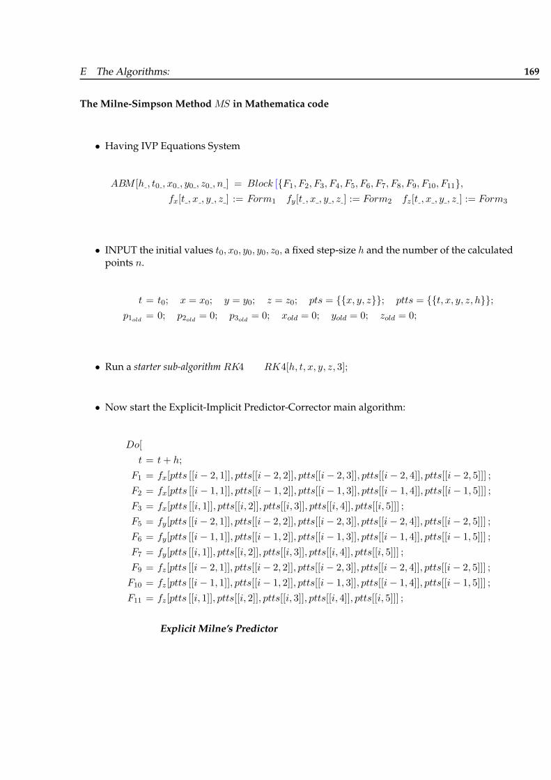
E The Algorithms: 169
The Milne-Simpson Method MS in Mathematica code
• Having IVP Equations System
ABM [h , t0 , x0 , y0 , z0 , n ] = Block [F1, F2, F3, F4, F5, F6, F7, F8, F9, F10, F11,fx[t , x , y , z ] := Form1 fy[t , x , y , z ] := Form2 fz[t , x , y , z ] := Form3
• INPUT the initial values t0, x0, y0, y0, z0, a fixed step-size h and the number of the calculatedpoints n.
t = t0; x = x0; y = y0; z = z0; pts = x, y, z; ptts = t, x, y, z, h;p1old
= 0; p2old= 0; p3old
= 0; xold = 0; yold = 0; zold = 0;
• Run a starter sub-algorithm RK4 RK4[h, t, x, y, z, 3];
• Now start the Explicit-Implicit Predictor-Corrector main algorithm:
Do[t = t+ h;
F1 = fx[ptts [[i− 2, 1]], ptts[[i− 2, 2]], ptts[[i− 2, 3]], ptts[[i− 2, 4]], ptts[[i− 2, 5]]] ;F2 = fx[ptts [[i− 1, 1]], ptts[[i− 1, 2]], ptts[[i− 1, 3]], ptts[[i− 1, 4]], ptts[[i− 1, 5]]] ;F3 = fx[ptts [[i, 1]], ptts[[i, 2]], ptts[[i, 3]], ptts[[i, 4]], ptts[[i, 5]]] ;F5 = fy[ptts [[i− 2, 1]], ptts[[i− 2, 2]], ptts[[i− 2, 3]], ptts[[i− 2, 4]], ptts[[i− 2, 5]]] ;F6 = fy[ptts [[i− 1, 1]], ptts[[i− 1, 2]], ptts[[i− 1, 3]], ptts[[i− 1, 4]], ptts[[i− 1, 5]]] ;F7 = fy[ptts [[i, 1]], ptts[[i, 2]], ptts[[i, 3]], ptts[[i, 4]], ptts[[i, 5]]] ;F9 = fz[ptts [[i− 2, 1]], ptts[[i− 2, 2]], ptts[[i− 2, 3]], ptts[[i− 2, 4]], ptts[[i− 2, 5]]] ;F10 = fz[ptts [[i− 1, 1]], ptts[[i− 1, 2]], ptts[[i− 1, 3]], ptts[[i− 1, 4]], ptts[[i− 1, 5]]] ;F11 = fz[ptts [[i, 1]], ptts[[i, 2]], ptts[[i, 3]], ptts[[i, 4]], ptts[[i, 5]]] ;
Explicit Milne’s Predictor

170 Appendix
p1new = ptts[[i− 3, 2]] +4h3
(2F1 − F2 + 2F3) ;
p2new = ptts[[i− 3, 3]] +4h3
(2F5 − F6 + 2F7) ;
p3new = ptts[[i− 3, 4]] +4h3
(2F9 − F10 + 2F11) ;
p1mod= p1new +
28 (xold − p1old)
29;
p2mod= p2new +
28 (yold − p2old)
29;
p3mod= p3new +
28 (zold − p3old)
29;
F0 = fx[t, p1mod, p2mod
, p3mod];
F4 = fy[t, p1mod, p2mod
, p3mod];
F8 = fz[t, p1mod, p2mod
, p3mod];
Implicit Simpson’s Corrector
x = ptts[[i− 1, 2]] +h
3(F2 + 4F3 + F0) ;
y = ptts[[i− 1, 3]] +h
3(F6 + 4F7 + F4) ;
z = ptts[[i− 1, 4]] +h
3(F10 + 4F11 + F8) ;
pts = AppendTopts, x, y, z; ptts = AppendToptts, t, x, y, z, h;p1old
= p1new ; p2old= p2new ; p3old
= p3new ; xold = x; yold = y; zold = z;F1 = F2; F2 = F3; F3 = fx[t, x, y, z]; F5 = F6; F6 = F7;F7 = fy[t, x, y, z]; F9 = F10; F10 = F11; F11 = fz[t, x, y, z], i, 4, n
Print[” ”];Print[”The Adams−Bashforth−Moulton methotd is used with ”, n, ” subintervals.”];
]

E The Algorithms: 171
The Hamming’s Method in Mathematica code
• Having IVP Equations System
Ham[h , t0 , x0 , y0 , z0 , n ] = Block [F1, F2, F3, F4, F5, F6, F7, F8, F9, F10, F11,fx[t , x , y , z ] := Form1 fy[t , x , y , z ] := Form2 fz[t , x , y , z ] := Form3
• INPUT the initial values t0, x0, y0, y0, z0, a fixed step-size h and the number of the calculatedpoints n.
t = t0; x = x0; y = y0; z = z0; pts = x, y, z; ptts = t, x, y, z, h;p1old
= 0; p2old= 0; p3old
= 0; c1old= 0; c2old
= 0; c3old= 0;
• Run a starter sub-algorithm RK4 RK4[h, t, x, y, z, 3];
• Now start the Explicit-Implicit Predictor-Corrector main algorithm:
Do[t = t+ h;
F1 = fx[ptts [[i− 2, 1]], ptts[[i− 2, 2]], ptts[[i− 2, 3]], ptts[[i− 2, 4]], ptts[[i− 2, 5]]] ;F2 = fx[ptts [[i− 1, 1]], ptts[[i− 1, 2]], ptts[[i− 1, 3]], ptts[[i− 1, 4]], ptts[[i− 1, 5]]] ;F3 = fx[ptts [[i, 1]], ptts[[i, 2]], ptts[[i, 3]], ptts[[i, 4]], ptts[[i, 5]]] ;F5 = fy[ptts [[i− 2, 1]], ptts[[i− 2, 2]], ptts[[i− 2, 3]], ptts[[i− 2, 4]], ptts[[i− 2, 5]]] ;F6 = fy[ptts [[i− 1, 1]], ptts[[i− 1, 2]], ptts[[i− 1, 3]], ptts[[i− 1, 4]], ptts[[i− 1, 5]]] ;F7 = fy[ptts [[i, 1]], ptts[[i, 2]], ptts[[i, 3]], ptts[[i, 4]], ptts[[i, 5]]] ;F9 = fz[ptts [[i− 2, 1]], ptts[[i− 2, 2]], ptts[[i− 2, 3]], ptts[[i− 2, 4]], ptts[[i− 2, 5]]] ;F10 = fz[ptts [[i− 1, 1]], ptts[[i− 1, 2]], ptts[[i− 1, 3]], ptts[[i− 1, 4]], ptts[[i− 1, 5]]] ;F11 = fz[ptts [[i, 1]], ptts[[i, 2]], ptts[[i, 3]], ptts[[i, 4]], ptts[[i, 5]]] ;
Explicit Hamming’s Predictor

172 Appendix
p1new = ptts[[i− 3, 2]] +4h3
(2F1 − F2 + 2F3) ;
p2new = ptts[[i− 3, 3]] +4h3
(2F5 − F6 + 2F7) ;
p3new = ptts[[i− 3, 4]] +4h3
(2F9 − F10 + 2F11) ;
p1mod= p1new +
112 (c1old− p1old
)121
;
p2mod= p2new +
112 (c2old− p2old
)121
;
p3mod= p3new +
112 (c3old− p3old
)121
;
F0 = fx[t, p1mod, p2mod
, p3mod];
F4 = fy[t, p1mod, p2mod
, p3mod];
F8 = fz[t, p1mod, p2mod
, p3mod];
Implicit Hamming’s Corrector
c1new =18
(9 ptts[[i, 2]]− ptts[[i− 2, 2]]) +3h8
(−F2 + 2F3 + F0);
c2new =18
(9 ptts[[i, 3]]− ptts[[i− 2, 3]]) +3h8
(−F6 + 2F7 + F4);
c3new =18
(9 ptts[[i, 4]]− ptts[[i− 2, 4]]) +3h8
(−F10 + 2F11 + F8);
x = c1new +9
121(p1new − c1new) ;
y = c2new +9
121(p2new − c2new) ;
z = c3new +9
121(p3new − c3new) ;
pts = AppendTopts, x, y, z;ptts = AppendToptts, t, x, y, z, h;p1old
= p1new ; p2old= p2new ; p3old
= p3new ; c1old= c1new ; c2old
= c2new ; c3old= c3new ;
F1 = F2; F2 = F3; F3 = fx[t, x, y, z]; F5 = F6;F6 = F7; F7 = fy[t, x, y, z]; F9 = F10; F10 = F11; F11 = fz[t, x, y, z], i, 4, n
Print[” ”];Print[”The Hamming′s methotd is used with ”, n, ” subintervals.”];
]

E The Algorithms: 173
E.4 Multi-step methods: variable step-size
The Adams-Bashforth-Moulton Variable step-size Method ABMV in Mathematica code
• Having IVP Equations System
ABMV [h , t0 , x0 , y0 , z0 , n ] = Block [F1, F2, F3, F4, F5, F6, F7, F8, F9, F10, F11,fx[t , x , y , z ] := Form1 fy[t , x , y , z ] := Form2 fz[t , x , y , z ] := Form3
• INPUT the initial values t0, x0, y0, y0, z0, a fixed step-size h and the number of the calculatedpoints n.
hmax = 64h; hmin =164h; Tol = 10−10; t = t0; x = x0; y = y0; z = z0;
h = hmax; pts = x, y, z; ptts = t, x, y, z, h;
• Run a starter sub-algorithm RK4 RK4[h, t, x, y, z, 3];
• Now start the Explicit-Implicit Predictor-Corrector main algorithm:
Do[t = t+ h;
F0 = fx[ptts [[i− 3, 1]], ptts[[i− 3, 2]], ptts[[i− 3, 3]], ptts[[i− 3, 4]], ptts[[i− 3, 5]]] ;F1 = fx[ptts [[i− 2, 1]], ptts[[i− 2, 2]], ptts[[i− 2, 3]], ptts[[i− 2, 4]], ptts[[i− 2, 5]]] ;F2 = fx[ptts [[i− 1, 1]], ptts[[i− 1, 2]], ptts[[i− 1, 3]], ptts[[i− 1, 4]], ptts[[i− 1, 5]]] ;F3 = fx[ptts [[i, 1]], ptts[[i, 2]], ptts[[i, 3]], ptts[[i, 4]], ptts[[i, 5]]] ;F4 = fy[ptts [[i− 3, 1]], ptts[[i− 3, 2]], ptts[[i− 3, 3]], ptts[[i− 3, 4]], ptts[[i− 3, 5]]] ;F5 = fy[ptts [[i− 2, 1]], ptts[[i− 2, 2]], ptts[[i− 2, 3]], ptts[[i− 2, 4]], ptts[[i− 2, 5]]] ;F6 = fy[ptts [[i− 1, 1]], ptts[[i− 1, 2]], ptts[[i− 1, 3]], ptts[[i− 1, 4]], ptts[[i− 1, 5]]] ;F7 = fy[ptts [[i, 1]], ptts[[i, 2]], ptts[[i, 3]], ptts[[i, 4]], ptts[[i, 5]]] ;F8 = fz[ptts [[i− 3, 1]], ptts[[i− 3, 2]], ptts[[i− 3, 3]], ptts[[i− 3, 4]], ptts[[i− 3, 5]]] ;F9 = fz[ptts [[i− 2, 1]], ptts[[i− 2, 2]], ptts[[i− 2, 3]], ptts[[i− 2, 4]], ptts[[i− 2, 5]]] ;F10 = fz[ptts [[i− 1, 1]], ptts[[i− 1, 2]], ptts[[i− 1, 3]], ptts[[i− 1, 4]], ptts[[i− 1, 5]]] ;F11 = fz[ptts [[i, 1]], ptts[[i, 2]], ptts[[i, 3]], ptts[[i, 4]], ptts[[i, 5]]] ;

174 Appendix
Explicit Adams-Bashforth Predictor
p1 = x+h
24(−9F0 + 37F1 − 59F2 + 55F3) ;
p2 = x+h
24(−9F4 + 37F5 − 59F6 + 55F7) ;
p3 = x+h
24(−9F8 + 37F9 − 59F10 + 55F11) ;
Implicit Adams-Moulton Corrector
c1 = x+h
24(F1 − 5F2 + 19F3 + 9fx[t, p1, p2, p3, p4]) ;
c2 = x+h
24(F5 − 5F6 + 19F7 + 9fy[t, p1, p2, p3, p4]) ;
c3 = x+h
24(F9 − 5F10 + 19F11 + 9fz[t, p1, p2, p3, p4]) ;
σ =19h270
√(c1 − p1)2 + (c2 − p2)2 + (c3 − p3)2;
If [σ 6= 0,
δ = 0.84(Tol
σ
) 14
;
If [δ > 4, h = 4h, h = δ h];If [δ < .1, h = .1h, h = .7δ h];If [h > hmax, h = .313hmax];If [h < hmin, Break[ ]];];If [δ ≤ Tol,
x = c1; y = c2; z = c3;pts = AppendTopts, x, y, z;ptts = AppendToptts, t, x, y, z, h], i, 4, n];Print[” ”];Print[”The V araible−step Adams−Bashforth−Moulton method is used with ”, n, ” subintervals.”];
]

175
Bibliography
[1] Richard Feynmann, The Feynmann Lectures on Physics, Volume 2, Benjamin Cummings 1963,ISBN: 0-201-02117-X
[2] H. Hertz, Die Krafte electrischer Schwingungen, behandelt nach der Maxwell’schen Theorie, An-nalen der Physik und Chemie 1889
[3] Warren L. Stutzman, Gary A. Thiele Antenna theory and design John Wiley & Sons,Inc, NewYork, 1981
[4] P. Lorraine, D.P. Corson, F. Lorraine, Electromagnetic Fields and Waves W.H. Freeman andcompany, New York
[5] Zuhrt H. “Electromagnetic radiation fields”, Springer 1953”
[6] Arfken, G. Mathematical Methods for Physicists, 3rd ed. Orlando, FL: Academic Press, pp. 198-200, 1985.
[7] Goldstein, H. “The Euler Angles” and “Euler Angles in Alternate Conventions. ” §4-4 and AppendixB in Classical Mechanics, 2nd ed. Reading, MA: Addison-Wesley, pp. 143-148 and 606-610, 1980.
[8] Landau, L. D. and Lifschitz, E. M. Mechanics, 3rd ed. Oxford, England: Pergamon Press, 1976.
[9] Margenau, H. and Murphy, G. M. The Mathematics of Physics and Chemistry, 2 vols. Princeton,NJ: Van Nostrand, 1956-64.
[10] Osgood, W. F. Mechanics. New York: Macmillan, 1937.
[11] Tuma, J. J. Dynamics. New York: Quantum Publishers, 1974.
[12] Varshalovich, D. A.; Moskalev, A. N.; and Khersonskii, V. K. “Description of Rotation inTerms of the Euler Angles. ”§1.4.1 in Quantum Theory of Angular Momentum. Singapore:World Scientific, pp. 21-23, 1988.
[13] MATHWORLD Website http://mathworld.wolfram.com/EulerAngles.html
[14] G. Monich Correlation between Gain and Wave Propagation in the Aperture Region of long trans-mitting Yagi-Uda -Antennas Int. URSI Symposium 1980, Munich Aug. 26. to 29.

176 Bibliography
[15] C.A. Balanis, Antenna Theory, Analysis and Design John Wiley and Sons, New York
[16] Butcher, J. C., “Numerical Methods for Differential Equations” John Wiley and Sons 2003.
[17] R. L. Burden. J. D. Faires, Numerical Analysis. 5th Ed. PWS Publishing Company Boston 1993.
[18] J. H. Mathews, Numerical Methods Using MATLAB, 3rd Ed, 1999, Prentice Hall. Inc.
[19] L. F. Shampine, Numerical Solution of Ordinary Differential Equations, Chapman and Hall, 1994.

177
Index
Index
Accuracy, 150algorithms, 161
- Multi-step methods, 167Adams-Bashforth-Moulton Method, 167Hamming’s Method, 171Milne-Simpson Method, 169variable Adams-Bashforth-Moulton Method,
173- One-step methods, 161
Euler’s Method , 161Heun’s Method , 161Runge-Kutta Method , 162Runge-Kutta-Fehlberg Method , 163
antenna- linear dipole , xiii- lines of force, xiii
field lines, xiii- Radiation Patterns, xiv- the image theory, xiv
antennas- the image theory, 35
arbitrarily oriented- finite length, 70
electric, 70magnetic, 70
- Hertzian, 69Electric, 69Magnetic, 69
- Radiators, 57
Big O notation, 152Biot-Savart Law, 7
continuity equation, 18
density- current ~J , 5- electric charge ρe, 5, 18- electric current Je, 18- magnetic charge ρm, 18- magnetic current Jm, 18- magnetic flux ~B, 7
detaching- points, 6- process, 5
dipole- finite length, 4- Hertzian , xiv- radiation, xiii
duality, 28
EM- Radiation, 2- experimental confirmation, 17- spectrum, 17
excitation, 22
field- detachment, 4- retardation effect, 9
frequency domain, 22
H. Hertz, 29hodograph, 43
Jacobian matrix, 157
loop- kidney-shaped , 4- small, 4
Maxwell’s

178 Index
- Ampere Equation, 10- classes and forms, 15- differential Equations, 18- Equations, 15- integral Equations, 19- integro-differential equations, 17, 22
nonperiodic, 23Numerical
- approximate derivatives , 150- Approach, 73- Phenomenon of Stiffness, 156- Stability, 154- Stiffness, 154
phasor- notation, 22
Picard, 154plane
- meridian , xiiipolarization, 4
Radiation- single wire, 2
Replacement Rules, 58Rotation Matrix, 60
single wire- charge, 2- time-harmonic applications, 2- time-varying current, 2
superposition, 23symmetry
- surfaces, 38
Taylor, 149The longitudinal sectors’ approach, 29time domain function, 23
walls- E-wall (electric), 35- H-wall (magnetic), 35


![Exploring Time-Varying Multivariate Volume Data ...cwang11/research/vis18-mism.pdfinteractive storyboard for overall time-varying data visualization and feature exploration [26], attribute](https://img.pdfslide.net/doc/110x75/603cf831cf6b28692c27e22f/exploring-time-varying-multivariate-volume-data-cwang11researchvis18-mismpdf.jpg)