On the Zeros and Poles of a Transfer Function* · 2016-12-16 · ZEROS AND POLES OF A TRANSFER FUNCTION 127 of the language can be avoided in that case by identifying the “complex

On the Zeros and Poles of a Transfer Function*

Bostwick F. Wyman

Mathematics Department The Ohio State University 231 West 18th Avenue Columbus, Ohio 43210

Michael K. Sain

Department of Electrical and Computer Engineering University of Notre Dame Notre Dame, Indiana 46556

Giuseppe Conte

Institute of Mathematics University of Genova 16132 Genova, Italy

Anna-Maria Perdon

Department of Mathematical Methods and Models University of Padua 35100 Padua, Italy

Submitted by Jan C. WiUems

ABSTRACT

The poles and zeros of a linear transfer function can be studied by means of the pole module and the transmission zero module. These algebraic constructions yield finite dimensional vector spaces whose dimensions are the number of poles and the

*The work of Sain was partially supported by the Ohio State University Distinguished Visiting Professor program, by the University of Notre Dame’s Frank M. Freimann Chair in Electrical Engineering, and by the NSF under grant ECS-8405714. Tne work of Conte and Perdon was partially supported by the Ohio State University, by the C.N.R. and the Italian Ministry of Public Instruction, by the Fulbrighl Program, and by NATO.

LINEAR ALGEBRA AND ITS APPLICATIONS 122/123/124:123-144 (1989) 0 Elsevier Science Publishing Co., Inc., 1989

123

655 Avenue of the Americas, New York, NY 10010 0024-3795/89/$3.50

124 BOSTWICK F. WYMAN ET AL.

number of multivariable zeros of the transfer function. In addition, these spaces carry the structure of a module over a ring of polynomials, which gives them a dynamical or state space structure. The analogous theory at infinity gives finite dimensional spaces which are modules over the valuation ring of proper rational functions. Following ideas of Wedderbum and Fomey, we introduce new finite dimensional vector spaces which measure generic zeros which arise when a transfer function fails to be injective or surjective. A new exact sequence relates the global spaces of zeros, the global spaces of poles, and the new generic zero spaces. This sequence gives a structural result which can be summarized as follows: “The number of zeros of any transfer function is equal to the number of poles (when everything is counted appropriately).” The same result unifies and extends a number of results of geometric control theory by relating global poles and zeros of general (possibly improper) transfer functions to controlled invariant and controllability subspaces (including such spaces at infinity).

1. INTRODUCTION

In this paper we show that two problems in the foundations of linear system theory are surprisingly closely related, and we present a common solution. The two problems we have in mind can be summarized as “guiding principles,” or perhaps “fond hopes,” as follows:

(A) The number of zeros of a transfer function is equal to the number of poles.

(B) The zeros of a transfer function appear as unavoidable poles in feedback problems with constraints.

In this form, these principles seem vague, or wrong, or both. The first goal of our work must be to make sense out of these statements, deciding what to count as zeros and poles, and in what sense zeros appear as poles. Further- more, since our point of view is algebraic and structural, rather than computational, we will be seeking isomorphisms of algebraic objects, rather than just equality of dimensions or eigenvalues, for example.

It is known that in general the number of poles of a transfer function G(Z) (counting both the finite poles and the poles at infinity) may be greater than the number of zeros (so counted). The difference has been called the “defect” of the transfer function [6; 11, p. 4601. So what hope is there for guiding principle (A)? In fact, the defect has been calculated in terms of “Kronecker indices” or “ Wedderbum numbers” [6; 22; 11, Theorem 6.5-11, p. 4611. We maintain that these Wedderbum numbers are in fact the dimensions of new finite dimensional vector spaces which measure the size of two sorts of “generic zeros”: those arising from the failure of G(z) to be injective, and from the failure of G(z) to be surjective. Furthermore, the

ZEROS AND POLES OF A TRANSFER FUNCTION 125

number of ordinary “lumped” zeros is best viewed as the dimension of a zero module (either finite or at infinity) [2; 1820; 25-29; 12, p. 1131, and of course the number of poles is the dimension of the pole module, or minimal realization state space (possibly at infinity) [2; 8; 9, Chapter 10; 161. Guiding principle (A) becomes an exact sequence relating the usual pole modules, the lumped zero modules, and the new generic zero modules.

Next we turn to study of feedback in the presence of constraints, which is just one view of the Geometric Control Theory of Wonham, Morse, Basile, and Marro [23]. Consider a linear system with state space X, input space U, output space Y, dynamics map A: X + X, and input and output maps B : U + X, C: X + Y. We consider subspaces of the output kernel ker C, thinking of Cx = 0 as a linear constraint on the state space. In the geometric theory we seek feedbacks F : X -+ U such that the space ker C is (A + BF> invariant. If this is not achievable, at least we can find the maximal controlled invariant space V* c ker C which does admit such an F. That is, V* is the largest space admitting feedbacks which preserve the constraints given by C. Within V* there is the maximal controllability subspace R* within which poles can be moved at will using “friendly feedbacks”: those which preserve the constraints. That is, the factor space V*/R* measures poles of the original system which cannot be moved using friendly feedbacks. (The expert will recognize immediately that we are omitting many details). It has been known for a long time that these immovable poles coincide numerically with multivariable zeros [23, pp. 112%1131, and in a paper in this journal [26] this numerical fact was converted into an explicit module isomorphism. To summarize, let G(Z) be a strictly proper transfer function with transmission zero module Z(G), and let X be the pole module. Then there is a natural polynomial module isomorphism between Z(G) and the space V*/R* associated to the minimal realization of G(z).

Since the isomorphism of [26] depends very strongly on the fact that G(x) is strictly proper, it is reasonable to seek a corresponding result for improper transfer functions. Inspired by known connections between zeros at infinity and geometric control theory [l], the note 1191 gave some preliminary results and conjectures relating zeros and poles in the improper case. The present paper reorganizes and completes these ideas by using the new generic zero spaces to establish an explicit relationship between zeros and poles for general transfer functions. In this way we generalize the earlier connections with geometric control theory and give substance to guiding principle (B). In the end, it turns out that our two guiding principles coincide, giving one theorem.

The present paper is organized as follows: Section 1’ is a second introduction which discusses the algebraic methodology of the paper, inspired by the referee of an earlier version. Section 2 recalls basic notation and definitions of


the standard zero and pole modules. Section 3 presents the Wedderbum- Forney construction which leads to the spaces of generic zeros mentioned above. Section 4 discusses generic zeros arising from the kernel of a transfer function, and gives some relationships with the geometric theory. Section 5 contains the fundamental exact sequence which is the main result of this paper. Section 6 relates the global zero space and the Wedderbum-Fomey construction to the theory of minimal bases and dynamical indices. Section 7 includes a few comments about the connection between Wedderbum-Fomey spaces and modules of generic zeros.

1’. ALGEBRAIC INTRODUCTION

Our methods in this paper differ substantially from the usual methods of system theory in that we use routinely the methods and ideas of number theory and commutative algebra. We begin by assuming an arbitrary field k of coefficients, having in mind widely differing applications such as control systems (with k real or complex) or convolutional coding theory (with k finite). On the other hand, the present paper does not stress applications at all, but rather emphasizes the deep algebraic structure underlying k( z)-linear transformations. Here, we downplay our conviction that control engineering and coding theory (rather than pure algebra) have motivated the “correct” definitions of poles and zeros of matrices.

If k is an arbitrary field, then the choice of domain and range sets for the rational functions in k(z) is a little involved. In the complex theory, such functions are defined on, and take values in, the Riemann sphere. Given any complex rational function, we can count the multiplicity of pole or zero of that function at each point on the sphere. Such a counting function is called a valuation, and the idea of valuation extends to k(z) for any field k of scalars [13; 3; 6, Appendix)]. In a brief but very interesting note ([lo]; see also [ll, p. 4611) Kung and Kailath used valuations to study zeros of a matrix of rational functions. Although [lo] emphasized determinants, this paper was one of the inspirations for the original zero module definition in [25]. For more about the relationship of [lo] with the local theory of poles and zeros in Section 6 below, see [30, Section 41. Valuations of k(z) are given by all irreducible polynomials, together with the “point at infinity.” The new wrinkle is that there are irreducible polynomials over k which are not linear. Furthermore, the “value of a function at a point” (we identify a “point” with a valuation) need not be a member of the scalar field k, but rather lies in an extension of k, called a residue class field, defined by the corresponding polynomial. This theory applies to the real case, of course, but the full power


of the language can be avoided in that case by identifying the “complex valuations” with pairs of complex numbers. However, attention to the residue class fields is crucial for general fields, including finite fields. In particular, much of the classical polynomial matrix theory is involved with “rank drops” of matrices when functions are evaluated at a point. In general, evaluation of matrices of functions is done by factoring out the maximal ideal of a valuation ring to construct the residue class field. Lemmas 6.1 and 6.2 below deal with the rank drop issue, which was well understood from an algorithmic point of view.

Finally we would like to say a few words about the module theoretic approach to pole-zero theory. From the most naive point of view, a pole of a transfer function matrix is a pole of any of its coefficients, but this approach neglects the problem of assigning multiplicities and misses the possibility of numerically coincident poles and zeros which do not cancel. Some sophisti- cated approach is needed, and we settled on the pole module, or state space of the minimal realization. In our view, the dynamics of the system is captured by the action of a polynomial ring (or possibly a more general ring) on the state space. The module action is the dynamics. For polynomials, the module action is given by multiplication by the variable z, which gives a dynamics matrix A, whose eigenvalues are, in turn, the naive poles. The point at infinity has its own ring, and the study of modules over this ring leads to a clear understanding of generalized state space systems [16, 17, 2, 181. The multivariable zero module, defined in the next section, gives a state space object with its own dynamics (that is, its own module action) which, in the polynomial case, gives again eigenvalues which are the naive numerical zeros. We have argued at length elsewhere that the zero module is the “correct” embodiment of the (lumped, or finite dimensional) zeros. The present paper is a first attempt to understand the more compli- cated “generic” zeros using the Wedderbum-Forney construction.

2. NOTATION AND BASIC DEFINITIONS

Let k be a field, let k[ z] denote the ring of polynomials, and let k(z) denote the field of rational functions in the variable z. Denote by 0m the valuation ring at infinity of proper rational functions in k(z). If V is any finite dimensional vector space, write V(z) = V@ k( z), a vector space over k(z); fiV=V@k[z], a free module over k[z]; and s2,V=V@om, a free module over 0,. All tensor products are taken over the scalar field k. We will frequently also use the module of strictly proper vectors Z- l&V, and write V(Z) = 0V@zP’Q2,V. We denote the k-linear projections out of V(z) by


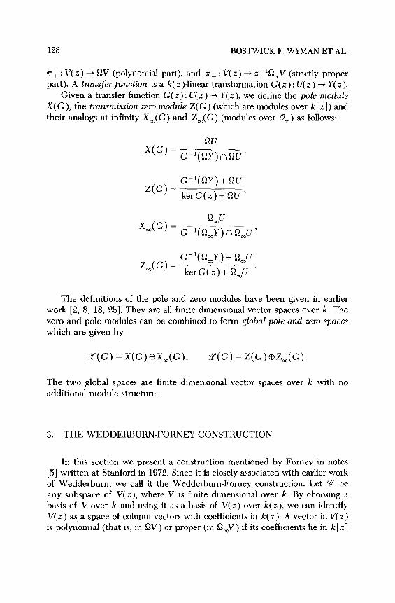
7~+ : V(z) + OV (polynomial part), and n_ : V(Z) + z-‘!J2,V (strictly proper part). A transfer finction is a k( z)-linear transformation G(Z) : U(z) + Y(Z).

Given a transfer function G(z): U(Z) + Y(Z), we define the pole module

X(G), the transmission zero module Z(G) (which are modules over k [ z]) and their analogs at infinity X,(G) and Z,(G) (modules over 0,) as follows:

Z(G) = G-‘(QY)+ !-NJ

kerG(z)+ QU ’

GAG> = G-l&Y)+ QJJ

kerG(z)+O,U ’

The definitions of the pole and zero modules have been given in earlier work [2, 8, 18, 251. They are all finite dimensional vector spaces over k. The zero and pole modules can be combined to form global pole and zero spaces which are given by

T(G) = X(G)@%,(G), 2(G) = Z(G)@Z,(G).

The two global spaces are finite dimensional vector spaces over k with no additional module structure.

3. THE WEDDERBURN-FORNEY CONSTRUCTION

In this section we present a construction mentioned by Forney in notes [5] written at Stanford in 1972. Since it is closely associated with earlier work of Wedderburn, we call it the Wedderburn-Forney construction. Let % be any subspace of V(Z), where V is finite dimensional over k. By choosing a basis of V over k and using it as a basis of V(Z) over k(.z), we can identify V(Z) as a space of column vectors with coefficients in k(z). A vector in V(z) is polynomial (that is, in QV) or proper (in !&V) if its coefficients lie in k[ Z]


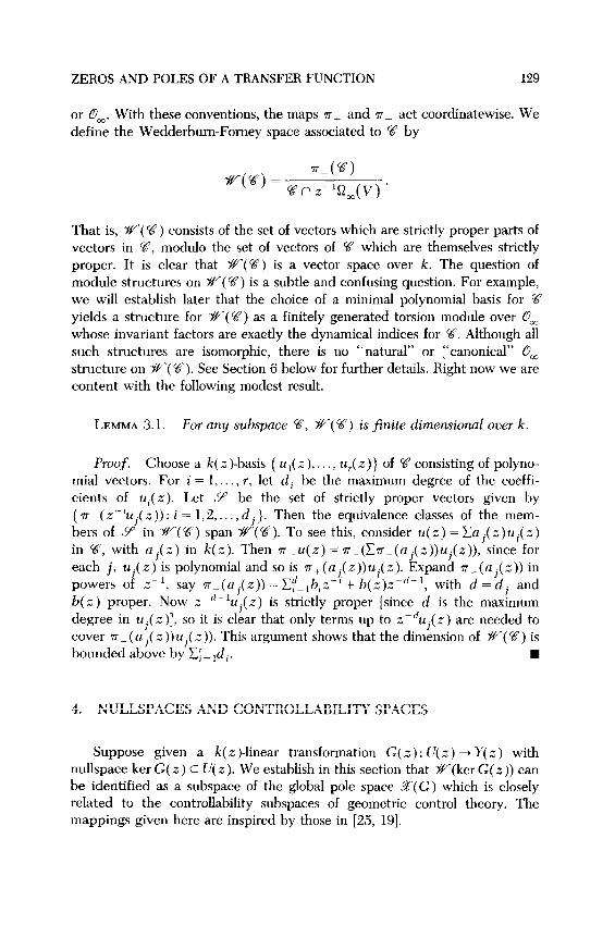
or om. With these conventions, the maps a, and n_ act coordinatewise. We define the Wedderbum-Fomey space associated to % by

That is, w(%‘) consists of the set of vectors which are strictly proper parts of vectors in %?, modulo the set of vectors of V which are themselves strictly proper. It is clear that w(U) is a vector space over k. The question of module structures on %‘“(V) is a subtle and confusing question. For example, we will establish later that the choice of a minimal polynomial basis for V yields a structure for %‘“(V) as a finitely generated torsion module over 0m whose invariant factors are exactly the dynamical indices for 9?. Although all such structures are isomorphic, there is no “natural” or :‘canonical” 0m structure on w(9). See Section 6 below for further details. Right now we are content with the following modest result.

LEMMA 3.1. For any subspace 9, W(W) is finite dimensional over k.

Proof. Choose a k( z )-basis { ui( z), . . , ur( z)} of % consisting of polynomial vectors. For i = 1,. . . , r, let d, be the maximum degree of the coefficients of u,(z). Let 9’ be the set of strictly proper vectors given by {a_(~-‘uj(z)): i = 1,2 ,..., dj}. Th en the equivalence classes of the mem- bers of 9’ in w(V) span w(V). To see this, consider U(Z) = Ca j(z)uj(z)

in %?, with a&z) in k(z). Then ~T_u(z) = a_(Ca_(aj(z))uj(z)), since for each j, uj(z) is polynomial and so is r+(ai(z))uj(.z). Expand r_(aj(z)) in powers of z- ‘, say rp(aj(z)) =Efxl_lbiz-’ + b(z)zp”-l, with d = dj and b( z ) proper. Now .z -“- ‘uj( z) is strictly proper [since d is the maximum degree in uj( z )], so it is clear that only terms up to z-%~( z ) are needed to cover 71~ (a j( z ))uj( z )). This argument shows that the dimension of ZJV( %‘) is bounded above by Cl= ,d i. w

4. NULLSPACES AND CONTROLLABILITY SPACES

Suppose given a k( z )-linear transformation G( .z) : U(z) + Y(z) with nullspace ker G( z) c U(z). We establish in this section that #‘-(ker G( 2)) can be identified as a subspace of the global pole space r(G) which is closely related to the controllability subspaces of geometric control theory. The mappings given here are inspired by those in [25, 191.


Note that since G(z) is k(z)-linear, we can write the definitions of the pole and zero modules at infinity in a way that uses strictly proper rather than proper inputs and outputs. This reformulation will simplify our later calculations.

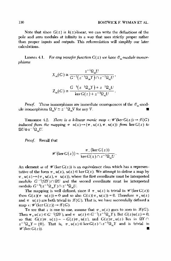
LEMMA 4.1. For any transfer function G(z) we have O,-module isomorphisms

Z,(G) iz G-I( z-‘G~Y) + z-‘C2JJ

kerG(z)+ z-‘L12,U ’

Proof. These isomorphisms are immediate consequences of the O,-module isomorphisms QJ E z- ‘C&V for any V. n

THEOREM 4.2. There is a k-linear rnonic map 1: w(ker G( z)) -+ .5?(G) induced from the mapping ~~u(~)H(~+u(z),~~u(z)) jbm kerG(z) to LxJ03z-‘~JL

Proof. Recall that

w(ker G( z)) = r_(kerG(z))

kerG(z)r\l z-‘f&U’

An element w of %‘-(ker G( z)) is an equivalence class which has a representative of the form r_ u(z), u(z) E ker G(z). We attempt to define a map by +rr ~ u(z) ++ (r + u( z), 7~ _ u(z)), where the first coordinate must be interpreted modulo G-r(QY) n G?U and the second coordinate must be interpreted modulo G-r(z-lQ,Y)n zPIL$JJ.

The mapping is well defined, since if a-u(z) is trivial in v(ker G(z)) then G(z)( 7~~ u(z)) = 0 and so also G( z)( 7~+ u( z)) = 0. Therefore r+ u( z) and 7~_ u(z) are both trivial in X(G). That is, we have successfully defined a map 1: -W(kerG(z)) + Z(G).

To see that 1 is one to one, assume that r_ u(z) goes to zero in X(G). Then T+U(Z) E G-‘(CJY), and a-~(z) E GP’(z-‘fi2,Y). But G(z)u(z) = 0, so that G(z)n_u(z)= - G(z)n+u(z), and Gnu lies in QY n z -‘Q2,Y = (0). That is, r-U(z)6 kerG(z)n z-‘&Y and is trivial in %‘-(ker G(z)). n


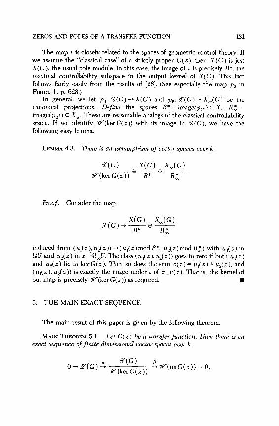
The map L is closely related to the spaces of geometric control theory. If we assume the “classical case” of a strictly proper G(z), then x(G) is just X(G), the usual pole module. In this case, the image of 1 is precisely R*, the maximal controllability subspace in the output kernel of X(G). This fact follows fairly easily from the results of [26]. (See especially the map p, in Figure 1, p. 628.)

In general, we let p,: 5(G)+ X(G) and p,: T(G)+ X,(G) be the canonical projections. Define the spaces R* = image(p,i) c X, Rz = image( p,h) C X,. These are reasonable analogs of the classical controllability space. If we identify W(ker G(z)) with its image in .%(G), we have the following easy lemma.

LEMMA 4.3. There is an isomorphism of vector spaces over k:

x(G) X(G) X,(G) W(kerG(x)) Z R* @ Rz ’

Proof. Consider the map

X(G) X,(G) .F(G)+F@-

RZ

induced from (~r(~),z+(~))+(~i(z)modR*, U,(z)modRz) with Us in L?U and us(z) in z-%&U. The class (u,(z), ~~(5)) goes to zero if both ur(.z) and us(z) lie in ker G(z). Then so does the sum V(Z) = ui(z) + u,(z), and (u r( z), us(z)) is exactly the image under 1 of 7~ _ v( z). That is, the kernel of our map is precisely W(ker G(Z)) as required. W

5. THE MAIN EXACT SEQUENCE

The main result of this paper is given by the following theorem.

MAIN THEOREM 5.1. Let G(z) be a transfer function. Then there is an exact sequence of finite dimensional vector spaces over k,


where

S“(G) is the global space of zeros of G(z); S(G) is the global space of poles of G(z); YV( ) is the “ Wedderburn-Forney ” construction.

Proof. We start with the map

To begin with, define a new space 27”,(G) (compare [14]) by

G-‘(QY)+ iHJ T”,(G)= au

~ G-1(z-‘i22,Y) + z-‘!&U

2 cc -% u

A typical element of %Or(G) has a representative of the form (u(z), o(z)), with G(z)u(z)~fIY and G(z)u(z)E zP’Q2,Y. The map we want will be induced from (u(z),D(z))~(~+(u(z)+ o(z)),~(u(z)+ v(z))) where the image shown gives a member of S?(G). This turns out to give a well-defined map from Zr(G) to X(G). Now, 2(G) comes from S!‘r(G) by “factoring out ker G( z),” and the map shown sends this kernel to W(ker G( z)) considered as a subspace of 2”(G). The upshot is that we have a well-defined injective map CY as required. To see this, consider the map

given by (u(z),D(z))~(~T+(u(z)+~(z)),~_(u(z)+w(z))). First we need to examine the effect of this map on vectors of the form (u(z),O), u(z) E G-‘(OY)f?QU, and (O,v(z)),v(z)~G-1(z-'~2,Y)nz~'~2,U. But according to the formula, (u(z),O) ++ (u( z),O), which is trivial in X(G), and (0, v(z)) c, (0, v(z)), trivial in X,(G). That is, the map shown gives a welldefined map (or: S’r(G) + a(G). To obtain S!‘“(G) from S“r(G), we must factor out the submodule of classes represented by vectors of the form (u(z), u(z)) where both u(z) and u( z ieinkerG(z).Thenalsou(z)+u(z) ) 1 lies in kerG(z), so (u(z),v(z)) goes to (P+(u(z)+ u(z)),‘TI_(u(z)+ v(z))),


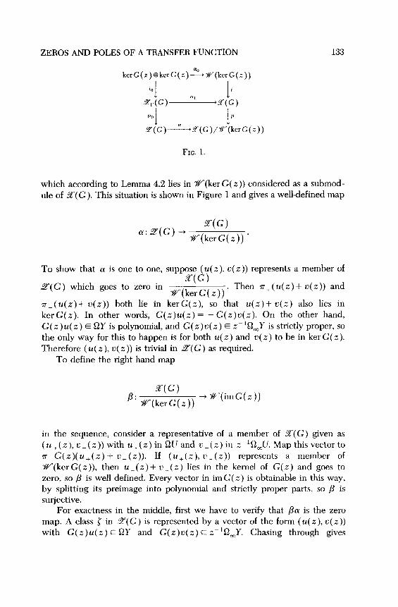
kerG(z)@kerG(z)&Y(kerC(;.))

i0 I

Tr(G) a’ Ii

,X(G)

PO

I I

P

I(G)-------~-----,~(G)/~(kerG(;))

FIG. 1.

which according to Lemma 4.2 lies in W(ker G( z)) considered as a submodule of 3(G). This situation is shown in Figure 1 and gives a welldefined map

To show that (Y is one to one, suppose (U(Z), u(z)) represents a member of

9’(G) which goes to zero in W(kerG(z)). Then r+(u(z)+ o(z)) and

a_(u(z)+u(z)) both lie in kerG(z), so that u(z)+u(z) also lies in ker G( z). In other words, G(x)u(z) = - G(.z)v(z). On the other hand, G( x)u( Z) E &?Y is polynomial, and G( Z)V( Z) E z-‘Q_,,Y is strictly proper, so the only way for this to happen is for both u(z) and V(Z) to be in ker G(z). Therefore (u( z ), v(z)) is trivial in S(G) as required.

To define the right hand map

T’(G) P: v(kerG(z)) + ~(imG(4)

in the sequence, consider a representative of a member of 3(G) given as (u+(z), u_(z)) with U+(Z) in OU and U-(Z) in zP’Q2,U. Map this vector to ~G(z)(u+(z) + K(Z)). If (U+(Z), V_(Z)) represents a member of W(ker G( z)), then u+(z) + u_(z) lies in the kernel of G( .z) and goes to zero, so p is well defined. Every vector in im G( Z) is obtainable in this way, by splitting its preimage into polynomial and strictly proper parts, so p is sujective.

For exactness in the middle, first we have to verify that /3& is the zero map. A class { in 5(G) is represented by a vector of the form (U(Z), U(Z)) with G(z)u(z) E OY and G(z)v(z) E zP1&Y. Chasing through gives


Pa(b)= ~G(z)r_$z) in w(imG(z)), which is zero, since G(z)u(s) is strictly proper, by the definition of the Wedderburn-Fomey construction.

Finally, we need to show that if ,8 kills a member of X(G)

w(kerG(.zll ’ then

\ that member lies in the image of (Y. Suppose given, then,‘a class having a representative (U +(z), z, _ (z)) with U+(Z) polynomial and o (z) strictly proper, killed by /?. Define r(z) = U+(Z) + v _(a). Then G( z)( r( z)) is strictly

proper, so (0, r(z)) represents a member of E.?“(G). But a((0, r(z)) = (7~+(r(~)),~_(r(~)))=(~+(~),n_(~)),sowearedone. n

This theorem has the following numerical corollary which inspired much of the development.

COROLLARY 5.2. Let G(z) be a transfer function. Then dim X(G) = dim z(G) + dim w(ker G(z)) + dim W(im G( z)).

This corollary, which follows immediately by counting dimensions, should be interpreted as stating that “the number of poles of a matrix of rational functions equals the number of zeros.” That is, the right hand side of the equation is a reasonable accounting of the total number of zeros of G(z).

We conclude this section by discussing the relationships between the main exact sequence and geometric control theory, following primarily [26, 191. Let us examine the injective map (Y using the notation of Lemma 4.3: Consider

X(G) X,(G) a:Z(G)~Zm(G)+R,@+--

Rz ’

This map (Y yields four maps when composed with the various inclusions and projections, of which the more important are

X(G) afin: Z(G) + 7 and

X,(G) (Y,: Z,(G) + ~

R; ’

The map efin was discussed in detail in [26] for strictly proper G(Z), and it was proved there that the image of ofi,, is exactly V*/R*, where V* is the maximal controlled invariant subspace of the output kernel. For arbitrary G(z), efiu gives a reasonable definition of a space V*. If we name the kernel of efi,, S(G), we have an exact sequence from [I91

O-,S(G)+Z(G)+V*/R*+O,


and recalling that (Y itself is injective, it is easy to identify S(G) as a subspace of Z,(G). Analogous remarks apply to Q, but rather than give details here, we refer the reader to [19] for a summary and promise to give an elaborate treatment in a later paper.

6. MINIMAL INDICES AND WEDDERBURN-FORNEY SPACES

In this section we study the Wedderburn-Forney spaces w(%?) for subspaces % of spaces of the form V(Z). Our goal is to recall earlier work on minimal indices and minimal polynomial bases, and use the main Theorem to give a unified approach to these issues. Our point of departure is Fomey’s seminal paper [6], although some of the main ideas were already done by Wedderbum and Kronecker [22; 12, p. 95-991.

We identify V(Z) as a space of column vectors with coefficients in k(x), and our first goal is to define the degree of a vector V(Z) = (o,(z),a,(z),..., a,(~))~. Let .!? be the set of all primes of k(z) [that is, the valuations of k(z) which are given by irreducible polynomials and the point at infinity] [4; 21, p. 133; 13, Chapter 1; 3, Section 11.51. For a prime p in B let ord, be the corresponding order function. The “product formula,” which is really a sum formula in the present notation [21, Theorem 3.3, p. 134; 61, states that C D c,ord,(f(z)) = 9 f or all f(z) in k(z). We extend the definition of ord, to V(Z) by ord,v(z)=min{ord,(ai(z)):i=1,2,...,n}. The failure of the product formula for vectors is measured by a positive integer called the degree (or sometimes the defect) of the vector: deg(u( z)) = -c v E B ord J v( z)) [4, p. 5191. The product formula shows immediately that the degree of a vector is a homogeneous invariant: that is, deg(a(x)v( z)) = deg( u(z)) for any nonzero u(z) in k(z). It is frequently convenient to multiply V(Z) by a least common denominator of its coefficients, and then to divide it by any common polynomial factor of those coefficients, thereby replacing it by a vector of polynomials with no common factor. In this case, calculation of the sum shows that the degree of u(z) is precisely the maximum of the degrees of the polynomial coefficients. This number can also be viewed as the degree of the curve in projective space defined by v(z) and as such is closely related to work of Hermann and Martin [21, Theorem 5.2, p. 139; 71.

Now, following Wedderbum and Forney, we are ready to use the degree function to describe a minimal basis of a subspace %? of V(x). If % = 0, stop. Otherwise, choose a vector cl(z) in q of least degree. Among the vectors of % linearly independent of cl(z), if any, choose a vector ca( z) of least degree, and continue until a basis is found. Such a basis is called a minimal basis. It


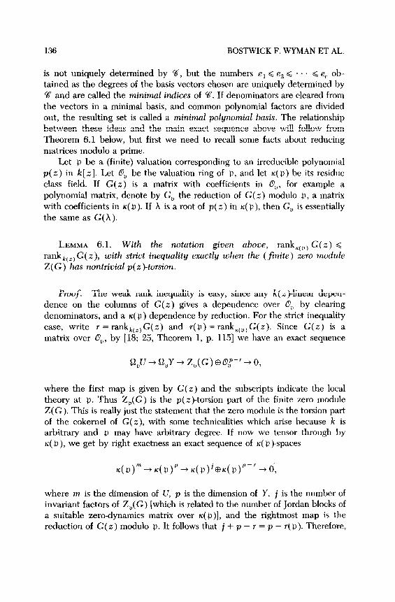
is not uniquely determined by %, but the numbers e, < e2 < . . . < e, ob- tained as the degrees of the basis vectors chosen are uniquely determined by 9? and are called the minimal indices of %?. If denominators are cleared from the vectors in a minimal basis, and common polynomial factors are divided out, the resulting set is called a minimal polynomial basis. The relationship between these ideas and the main exact sequence above will follow from Theorem 6.1 below, but first we need to recall some facts about reducing matrices modulo a prime.

Let p be a (finite) valuation corresponding to an irreducible polynomial p(z) in k [ z]. Let Ou be the valuation ring of n, and let K( 0) be its residue class field. If G(z) is a matrix with coefficients in Lo,,, for example a polynomial matrix, denote by G, the reduction of G(z) modulo n, a matrix with coefficients in K(P). If x is a root of p(z) in K( $I), then G, is essentially the same as G(A).

LEMMA 6.1. With the notation given above, rank.(,, G(z) < rankkC_, G( z), with strict inequality exactly when the (finite) zero module Z(G) has nontrivial p( z )-torsion.

Proof. The weak rank inequality is easy, since any k(z)-linear dependence on the columns of G(z) gives a dependence over O$, by clearing denominators, and a K( $I) dependence by reduction. For the strict inequality case, write r =rank,(,,G(z) and r(p)=rank,(,,G(z). Since G(z) is a matrix over O,, by [18; 25, Theorem 1, p. 1151 we have an exact sequence

where the first map is given by G(z) and the subscripts indicate the local theory at p. Thus Z,(G) is the p( z>torsion part of the finite zero module Z(G). This is really just the statement that the zero module is the torsion part of the cokemel of G(z), with some technicalities which arise because k is arbitrary and p may have arbitrary degree. If now we tensor through by K(Q), we get by right exactness an exact sequence of K( @)-spaces

where m is the dimension of U, p is the dimension of Y, j is the number of invariant factors of Z,(G) [which is related to the number of Jordan blocks of a suitable zero-dynamics matrix over K(#)], and the rightmost map is the reduction of G(z) modulo p. It follows that j + p - r = p - r( 0). Therefore,


r - r(p) = j, and we see that a rank drop occurs if and only if j > 0. Now j > 0 exactly when Z,(G) does not vanish, and we have established a quantitative form of the lemma. w

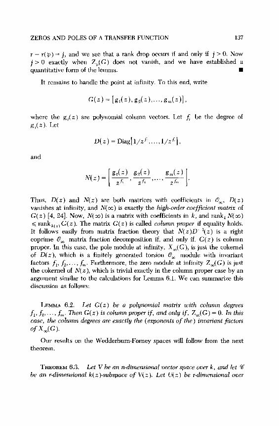
It remains to handle the point at infinity. To this end, write

G(z)= [gl(z),g,(z),...,g,(z)l,

where the g i( z ) are polynomial column vectors. Let f; be the degree of g,(z). Let

D(z) =Diag[l/zf’,...,l/~~],

and

Thus, D(z) and N(z) are both matrices with coefficients in 0%, D(z) vanishes at infinity, and N(co) is exactly the high-order coefficient matrix of G(z) [4, 241. Now, N(m) is a matrix with coefficients in k, and rankk N(cc) < rankkCz)G(z). The matrix G(z) is called column proper if equality holds. It follows easily from matrix fraction theory that N(z)D-‘(z) is a right coprime 0m matrix fraction decomposition if, and only if, G(z) is column proper. In this case, the pole module at infinity, X,(G), is just the cokemel of D(z), which is a finitely generated torsion Um module with invariant factors f,, fi,. . . , f,. Furthermore, the zero module at infinity Z,(G) is just the cokernel of N(z), which is trivial exactly in the column proper case by an argument similar to the calculations for Lemma 6.1. We can summarize this discussion as follows:

LEMMA 6.2. Let G(z) be a polynomial matrix with column degrees

fi>fi,..., f,. Then G(z) is column proper if, and only if, Z,(G) = 0. In this case, the column degrees are exactly the (exponents of the) invariant factors

of X,(G).

Our results on the Wedderbum-Fomey spaces will follow from the next theorem.

THEOREM 6.3. Let V be an n-dimensional vector space over k, and let V be an rdimensionul k(z)-subspace of V(z). Let U(z) be rdimensional over


k(z), and consider an injective transfer function G(z) : U(z) -+ V(z) with image SF?, viewed as an n x r matrix over k(z). Then the columns of G(z)

form a minimal basis of V if, and only if, the global zero space .3(G) is zero. The columns of G(z) form a polynomial basis of % if, and only if, the finite pole module X(G) is zero.

Proof. Since G(z) is injective with image %?, then the columns of G(z) surely form a basis of %. Also, G(z) is a polynomial matrix if and only if all the poles of G(z) occur at infinity, so the second statement of the theorem is obvious. The first statement of the theorem follows Fomey’s “Main Theorem” [4, pp. 495, 5191. According to Fomey, if G(z) is injective and polynomial, the columns of G( z ) give a minimal polynomial basis if and only if G(z) does not lose rank at any valuation (including co). However, according to Lemmas 6.1 and 6.2 this condition precisely coincides with the vanishing of %“( G ). n

This result, together with the main exact sequence of the present paper, gives us very precise information about the Wedderbum-Fomey spaces.

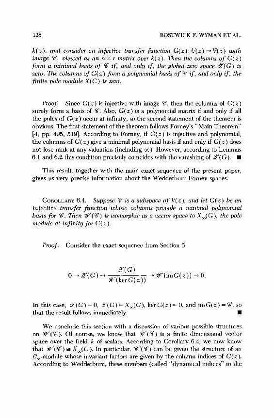
COROLLARY 6.4. Suppose V is a subspace of V(z), and let G(z) be an injective transfer function whose columns provide a minimal polynomial

basis for 97. Then W(V) is isomorphic as a vector space to X,(G), the pole module at infinity for G(z).

Proof. Consider the exact sequence from Section 5

In this case, T(G)=O, %(G)=X,(G), kerG(z )=O, and imG(z)=V, so that the result follows immediately. n

We conclude this section with a discussion of various possible structures on “w( Q?). Of course, we know that w(U) is a finite dimensional vector space over the field k of scalars. According to Corollary 6.4, we now know that $Y(Q?) = X,(G). In particular, w(U) can be given the structure of an Lo,-module whose invariant factors are given by the column indices of G(z). According to Wedderbum, these numbers (called “dynamical indices” in the


control literature) are uniquely determined by %2. We can restate the last

corollary as follows:

COROLLARY 6.5. Suppose %? is a subs-pace of V(z). The dimension of

W(V) is exactly the sum of the dynamical indices of 5%‘. For every minimal basis matrix G(z), W(g) can be given an Co,-module structure correspond-

ing to Xm( G), the pole module at infinity for G(z). All of these CO,-module

structures are isomorphic.

The proof of this lemma was done by appeal to Wedderbum. We do not know a “natural proof,” and in fact, we claim that there is no natural Oa

module structure on Y+‘-(V). Of course, we cannot prove such a statement without a rigorous definition of “natural structure,” but we present here an example to show what we have in mind.

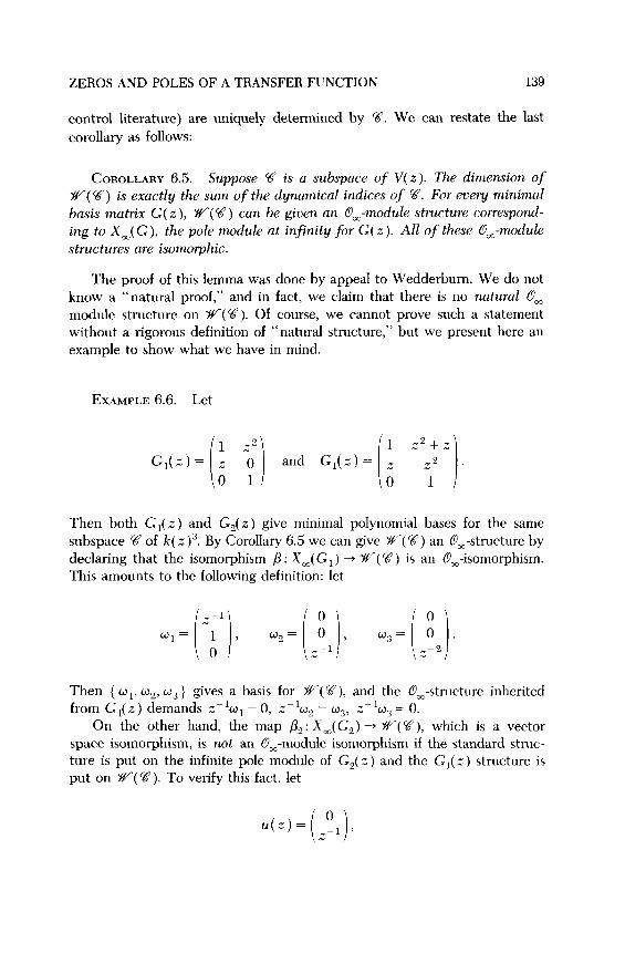
EXAMPLE 6.6. Let

Then both G,(z) and G,(z) give minimal polynomial bases for the same subspace $7 of k( z)~. By Corollary 6.5 we can give w( %’ ) an I0,-structure by declaring that the isomorphism /3: X,(G,) + %‘“(%?) is an Lo,o-isomorphism. This amounts to the following definition: let

Then { w r, w2, ws } gives a basis for YY( +?), and the 0S3-structure inherited from G,(z) demands zP1ol = 0, z-‘wz = wn, z-‘wa = 0.

On the other hand, the map & : X,(G,) + YY( F), which is a vector space isomorphism, is not an 0,-module isomorphism if the standard structure is put on the infinite pole module of G2( z) and the Gr(z) structure is put on YV(%?). To verify this fact, let


and consider &( u( z)) and &,( z- ‘u( z)). It is in this sense that we say that the Om-structure on w(V) is not a natural one.

Suppose given a space V as above. So far we have emphasized minimal polynomial bases, but in fact we can equally well consider minimal proper

bases. Thus, let G(z) be a proper injective transfer function with column space V. Consider once again the exact sequence from Section 5

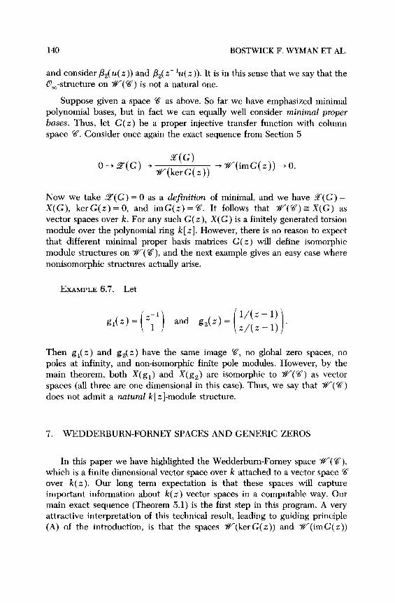
Now we take 2(G) = 0 as a definition of minimal, and we have x(G) = X(G), kerG(z)=O, and imG(.z)=%. It follows that w(V)= X(G) as vector spaces over k. For any such G(z), X(G) is a finitely generated torsion module over the polynomial ring k [ z]. However, there is no reason to expect that different minimal proper basis matrices G(z) will define isomorphic module structures on w(U), and the next example gives an easy case where nonisomorphic structures actually arise.

EXAMPLE 6.7. Let

and ga(z) =

Then gi(z) and gs(z) have the same image V, no global zero spaces, no poles at infinity, and non-isomorphic finite pole modules. However, by the main theorem, both X(gi) and X(gz) are isomorphic to %‘(%) as vector spaces (all three are one dimensional in this case). Thus, we say that w(q) does not admit a natural k[ z]-module structure.

7. WEDDERBURN-FORNEY SPACES AND GENERIC ZEROS

In this paper we have highlighted the Wedderbum-Forney space w(g), which is a finite dimensional vector space over k attached to a vector space %? over k(z). Our long term expectation is that these spaces will capture important information about k(z) vector spaces in a computable way. Our main exact sequence (Theorem 5.1) is the first step in this program. A very attractive interpretation of this technical result, leading to guiding principle (A) of the introduction, is that the spaces -W(ker G( z)) and %‘“(imG(z))


somehow measure zeros of a transfer function G(z) which are not captured by the classical transmission zero modules Z(G) and Z,(G). On the other hand, the work in Section 6 emphasized the interpretation of V(imG(z)) as a space of poles when certain minimality hypotheses hold. In this brief concluding section, we exhibit some connections between the Wedderburn- Fomey spaces and certain free or divisible modules of “generic zeros” which have proved to be important tools [14, 151.

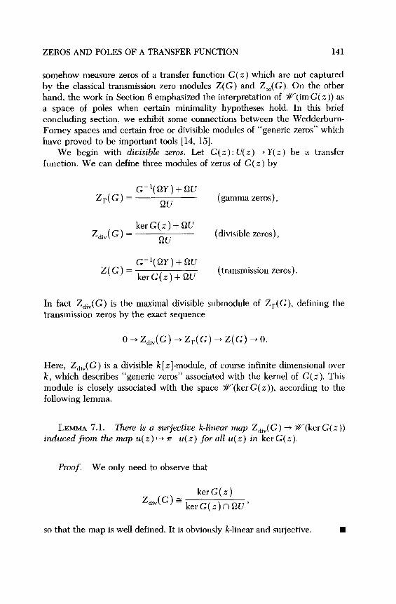
We begin with divisible zeros. Let G(z): U(z) + Y(z) be a transfer function. We can define three modules of zeros of G(z) by

G-‘(QY)+ OU Z,(G) = QU

(gamma zeros),

Z,,(G) = kerG(z) + OU

ou (divisible zeros),

Z(G) = G-‘(&Y)+ OU

kerG(z)+ OU (transmission zeros).

In fact Z,+(G) is the maximal divisible submodule of Z,(G), defining the transmission zeros by the exact sequence

O+Z,,(G)+Z,(G)+Z(G)+O.

Here, Z,.(G) is a divisible k[ z]-module, of course infinite dimensional over k, which describes “generic zeros” associated with the kernel of G(z). This module is closely associated with the space w(ker G(z)), according to the following lemma.

LEMMA 7.1. There is a surjective k-linear map Z,,(G) + w(ker G( z)) inducedfimn themapu(z)t,~_u(z)foraZZu(z) in kerG(z).

Proof. We only need to observe that

Z,iv(G> E kerG(z)

kerG(z)nQU’

so that the map is well defined. It is obviously k-linear and sujective. n


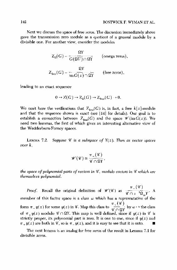
Next we discuss the space of free zeros. The discussion immediately above gave the transmission zero module as a quotient of a general module by a divisible one. For another view, consider the modules

GY Z,(G) =

G(W)nQY (omega zeros),

OY LY_w = imG(z)nQY

(free zeros),

leading to an exact sequence

O-,Z(G)+Z,(G)+Z,,,,(G)-0.

We omit here the verifications that Zfree(G) is, in fact, a free k[ z]-module and that the sequence shown is exact (see [lb] for details). Our goal is to establish a connection between Z ,,,,(G) and the space w(imG(z)). We need two lemmas, the first of which gives an interesting alternative view of the Wedderbum-Fomey spaces.

LEMMA 7.2. Suppose W is a subspace of Y(z). Then as vector spaces over k,

the space of polynomial parts of vectors in T?, module vectors in V which are themselves polynomial.

Proof. Recall the original definition of w(V) as d@)

gn z-‘0,Y’ A

member of this factor space is a class o which has a representative of the

r+(U) form a _ y(z) for some y(z) in ‘8. Map this class to E by w ++ the class

of 7~+ y(z) modulo %’ n QY. This map is well defined, since if y(z) in % is strictly proper, its polynomial part is zero. It is one to one, since if y(z) and v + y(x) are both in 59, so is r_ y(z), and it is easy to see that it is onto. n

The next lemma is an analog for free zeros of the result in Lemma 7.1 for divisible zeros.


LEMMA 7.3. There is an injective k-linear map w(im G( z )) + Zfree( G ) induced fimn the map y(z) ++ T+ y(z) for all y(z) in imG(z).

Proof. This map is well defined and one to one on w(imG(z)), since y( .z) goes to zero in Zfree(G) if, and only if, it is polynomial. n

Lemmas 7.1 and 7.3 give the promised connection between Wedderbum-Fomey spaces and generic zeros. We emphasize that these two results are easy and should be viewed as very preliminary. We do not yet know to what extent these finite dimensional spaces encapsulate the structure of the free and divisible modules of zeros, but we are confident that the Wedderbum-Forney spaces will be a rich source of interesting algebraic questions.

REFERENCES

1

2

3

8

9

10

11 12 13 14

C. Commault and J. Dion, Structure at infinity of linear multivariable systems: A geometric approach, IEEE Trans. Automat. Control AC-27:693-696 (1982). G. Conte and A. Perdon, Infinite zero module and infinite pole modules, in VII International Conference on Analysis and 0ptimi;ation of Systems: Nice, Lec- ture Notes in Control and Inform. Sci., 62, Springer, 1984, pp. 302-315. M. Eichler, Introduction to the Theory of Algebraic Numbers and Functions,

transl. by G. Striker, Academic, New York, 1966. 6. D. Forney, Jr., Convolutional codes I: Algebraic structure, IEEE Trans.

Inform. Theory IT-16:720-738 (1970). G. D. Fomey, Jr., unpublished notes, Stanford, 1972.

G. D. Forney, Jr., Minimal bases of rational vector spaces with applications to multivariable linear systems, SIAM J. Control 13:493-520 (1975). R. Hermann and C. Martin, Applications of algebraic geometry to systems theory: The McMillan degree and Kronecker indices of transfer functions, SIAM J. ConhoE 0ptim. 16:743-755 (1978). R. E. Kalman, Algebraic structure of linear dynamic systems. I. The module of sigma, Proc. Nat. Acad. Sci. U.S. A. 54:1503-1508 (1965). R. E. Kalman, P. Falb, and M. Arbib, Topics in Mathematical System Theory,

McGraw-Hill, New York, 1969, Chapter X. S. Kung and T. Kailath, Some notes on valuation theory in linear systems, in Proceedings of the 1978 IEEE Confmence on Decision und Control, San Diego, pp. 515-517. T. Kailath, Lineur Systems, Prentice-Hall, Englewood Cliffs, N.J., 1980. H. Rosenbrock, State Space and Multioariable Theory, Wiley, New York, 1970. 0. F. G. Schilling, The Theory of Valuations, Amer. Math. Sot., New York, 1950. M. K. Sain and B. Wyman, The fixed zero constraint in dynamical system performance, in Proceedings of the Eighth International Symposium on the


Mathematical Theory of Networks and Systems (C. I. Byrnes, C. F. Martin, and R. Saeks, Eds.), North-Holland, pp. 87-92.

15 M. Sain, B. Wyman, and J. Peczkowski, Zeros in plant specification: Constraints and solutions, in Proceedings of the American Control Confmence, June 1988, to appear.

16 G. Verghese, B. Levy, and T. Kailath, A generalized state space for singular systems, IEEE Trans. Automat. Control AC-26:811X331 (Aug. 1981).

17 G. Verghese, P. van Dooren, and T. Kailath, Properties of the system matrix of a generalized state-space system, Znternat. J. Control 30 (1979).

18 B. Wyman, G. Conte, and A. Perdon, “Local and Global Linear System Theory” in Frequency Domain and State Space Methods for Linear Systems (C. Byrnes and A. Lindquist, Eds.), North-Holland, Amsterdam, 1986, pp. 165-181.

19 B. Wyman, G. Conte, and A. Perdon, Zeropole structure of linear transfer functions, in Proceedings of the 1985 IEEE Decision and Control Conference, Fort Lauderdale.

20 B. Wyman, G. Conte, and A. Perdon, Fixed poles in transfer function equations, SIAM J. Control Cptim. 26:356368 (Mar. 1988).

21 R. J. Walker, Algebraic Curves, Dover, 1962 (reprinted from Princeton U. P., 1950).

22 J. H. M. Wedderburn, Lectures on Matrices, Amer. Math. Sot. Colloq. Publ. 17, 1934, Chapter 4.

23 M. Wonham, Linear M&variable Control: A Geometric Approach, 3rd ed., Springer, 1985.

24 W. Wolovich, Linear Multivariable Systems, Appl. Math. Sci. 11, Springer, New York, 1974.

25 B. Wyman and M. K. Sain, The zero module and essential inverse systems, IEEE

Trans. Circuits and Systems CAS-28:112-126 (1981). 26 B. Wyman and M. K. Sain, On the zeros of a minimal realization, Linear Algebra

Appl. 50:621-637 (1983). 27 B. Wyman and M. K. Sain, On the design of pole modules for inverse systems,

IEEE Trans. Circuits and Systems CAS-32:977-988 (1985). 28 B. Wyman and M. K. Sain, Module theoretic structures for system matrices,

SIAM J. Control Cptim. 25:86-99 (1987). 29 B. Wyman and M. K. Sain, Zeros of square invertible systems, in Proceedings of

the Eighth International Symposium on the Mathematical Theory of Networks and Systems (C. I. Bymes, C. F. Martin, and R. Saeks, Eds.), North-Holland, pp. 109- 114.

30 B. Wyman and M. K. Sain, A unified pole-zero module for linear transfer functions, Systems Control Lett. 5:117-120 (1984).

Received 8 June 1988; final manuscript accepted 19 September 1988

Documents

On the Zeros and Poles of a Transfer Function* · 2016-12-16 · ZEROS AND POLES OF A TRANSFER FUNCTION 127 of the language can be avoided in that case by identifying the “complex