On Use of Positive Feedback for Improved Torque

Control

Houman Dallali, Gustavo A. Medrano-Cerda,Michele Focchi, Thiago Boaventura, Marco Frigerio,

Claudio Semini, Jonas Buchli, and Darwin G. Caldwell, ∗†‡

September 25, 2014

Abstract

This paper considers the torque control problem for robots with flex-ible joints driven by electrical actuators. It is shown that the achievableclosed loop tracking bandwidth using PI torque controllers may be lim-ited due to transmission zeros introduced by the load dynamics. Thislimitation is overcome by using positive feedback from the load motion inunison with PI torque controllers. The positive feedback is given in termsof load velocity, acceleration and jerk. Stability conditions for designingdecentralized PI torque controllers are derived in terms of Routh-Hurwitzcriteria. Disturbance rejection properties of the closed system are charac-terized and an analysis is carried out investigating the use of approximatepositive feedback by omitting acceleration and/or jerk signals. The resultsof this paper are illustrated for a two DoF system. Experimental resultsfor a one DoF system are also included.

1 Introduction

Enhancing the bandwidth of torque tracking is one of the challenges in buildinghigh performance legged robots. The problem of increasing the torque band-width cannot be resolved by using faster actuators but it is related to the loadmotion rather than the actuator dynamics. This issue becomes more criticalwhen the load has little friction, i.e. good bearings are used at the point wherethe load is attached to the transmission. In the robotics community, many pub-lications on torque control have disregarded the load dynamics from the analysis[1, 2, 3] and this problem has been overlooked.

∗H Dallali, G. A. Medrano-Cerda, M. Focchi, M. Frigerio, C. Semini and D. G. Caldwellare with the Department of Advanced Robotics, Istituto Italiano di Tecnologia (IIT), Genova,Italy.

†T. Boaventura and J. Buchli are with Agile and Dexterous Robotics Lab, Institute ofRobotics and Intelligent Systems, ETH, Zurich, Switzerland.

‡Manuscript received September 25, 2014.

1

However bandwidth limitations in force control problems using hydraulicactuators have been reported in civil and automotive engineering. In [4] the in-teraction between the load motion and the actuator was shown for a hydraulicactuator. It was shown that a natural velocity feedback interaction path existsbetween the load (in that case a civil structure) and the actuator. Moreover,using a linearized model it was shown that the poles of the structure becomethe zeros of the open loop force transfer function. As a result, if the structureis lightly damped, the actuators will be unable to apply a force at the naturalfrequency of the structure, regardless of actuator dynamics speed (bandwidth).In [4] it was shown that the problem is not due to the actuator dynamics but dueto the structure (load) dynamics. In [5], experimental results of a car suspen-sion test rig were reported where a conventional PID controller was incapableof producing appropriate force tracking and resulted in a significant phase lagat frequencies higher than 1 Hz. The car test rig used very fast servo-valvedynamics to improve the force tracking performance but the problem was notresolved. In [6], the interaction between the hydraulic actuator and the struc-ture is discussed and an intuitive positive velocity feedback scheme is proposedto compensate for the load motion by negating the effect of the natural velocityfeedback. Despite simulation studies and experimental results, further analysisdetails on the effect of adding the positive feedback loop were not presented.Later in [7], several improvements were made to this method including the addi-tion of phase adjustment to the positive velocity feedback. Also the magnitudeof the positive velocity feedback was underestimated to avoid potential insta-bility. In [8] motor torque control was considered using a disturbance observerwhile no load was attached to the motor. In this work we are interested in torquecontrol at the joint and a system where the inertia is coupled via a compliantjoint. In [9], the authors showed how motion compensation can be applied toelectrically and hydraulically actuated joints of a quadruped robot called HyQ[10]. In [11], positive torque feedback was used to improve the problem of jointtracking, but it does not report the load motion problem. It was reportedthat positive joint torque feedback can compensate the detrimental effects ofload torques on position tracking performance. However, with non-ideal torquesources, simple unity gain positive torque feedback can actually deteriorate theperformance, or even result in instability.

Various complex control designs can be used for torque control. For instance,in [12] a combination of model based computed torque control, a state feedbackand a nonlinear H∞ was applied to a six DoF robot manipulator with jointflexibility. A high performance torque control method was implemented on alight weight robot arm in [13]. These methods need a good model and areimplemented in centralized architectures which places additional requirementson real-time communication among various Degrees of Freedom (DoF).

In practice, the use of decentralized PI controllers is widespread in robotics.PI controllers are easy to tune but have limitations in terms of tracking band-width and disturbance rejection. The main idea in this paper is to use de-centralized controllers by mitigating the existing limitations using quantifiedpositive feedback. The source of these limitations will be fully characterized for

2

multi-dof systems in terms of multi-variable zeros.The main contributions of this paper are the following: The role of positive

feedback is studied for mechanical systems driven with electric motors. It isshown that simple PI controllers can be used together with positive feedbackto significantly improve torque tracking performance. Stability conditions fordesigning decentralized PI torque controllers, when the positive feedback is ap-plied, are presented in terms of Routh-Hurwitz criteria. A two DoF case studyis used to illustrate the theory via root locus analysis and numerical simulations.Experimental results of a one DoF system are presented, validating the use ofpositive feedback.

The paper is organized as follows. Section 2, presents the system model andcharacterizes the corresponding multi-variable transmission zeros. Limitationson the achievable closed loop torque bandwidth are explained in terms of thetransmission zeros when using simple PI controllers. The use of positive feed-back is introduced and it is shown that this can be designed to decouple thejoint torque from the load dynamics. The positive feedback is given by threeterms involving load velocity, acceleration and jerk. General results to investi-gate closed loop stability when using this method are presented in section 2.4.Section 2.5, discusses disturbance rejection properties of the closed loop systemand in particular points out additional limitations when using PI torque con-trollers. In section 3, a case study based on a two DoF model is used to verifythe main results via nonlinear simulations and root locus analysis. In particular,the root locus analysis in section 3.4 investigates the effects of using a partialpositive feedback by neglecting load acceleration and/or jerk terms. Section 4presents some experimental results for one joint of a robot leg prototype [14].Concluding remarks are given in section 5.

Notation Throughout the paper, lower case letters are used for scalars, lowercase and bold letters are used for vectors and uppercase letters are used formatrices. Moreover, subscripts L and m refer to load and motor, respectively.

2 System Model and Main Results

This section presents the main results of the paper for the multi-Dof systemgiven by

ML(θL)θL + CL(θL,θL) +BLθL +G(θL) = τL + τLd, (1)

Jmθm +Bmθm +N−1τL = Kti+N−1τd, (2)

Li+Ri = vm −Kωθm, (3)

τL = KH

(N−1θm − θL

), (4)

where θL, θm, θL, θm are the angular positions and velocities of the loadand motor in relative coordinates; τL denotes the joint torque; τLd, τd aredisturbances acting on the link and motor; i and vm are the motors current

3

and voltage, respectively. The motor disturbance τd can represent meshingfriction and torque ripples produced by a reduction gearbox. We assume thatthe joint torque τL, the load and the motor positions are measured. Notehowever that one set of measurements is redundant since (4) provides a relationbetween them. A description of the system parameters is summarized in Table1. The motor equations in the model correspond to a DC permanent magnetmotor but as indicated by several motor manufacturers the same equations canbe used for DC brushless motors whenever these are appropriately commutated.Linearizing (1) at a given load position with zero angular velocity yields

MLθL +BLθL +KLθL = τL. (5)

where ML is obtained by evaluating the mass inertia matrix at a given loadposition and the linearized gravity vector KL is obtained by evaluating thepartial derivative of G at the given robot configuration.

Throughout the paper, the linearized model is used to investigate stabilityand disturbance rejection properties of the closed loop system when a PI torquecontroller is combined with positive feedback. The linearized analysis can beeasily repeated for several configurations of interest by generating a suitablemesh of the robot workspace. In this manner the closed loop performance ofthe robot can be investigated at different robot configurations. A case study willillustrate that the predicted performance using the linearized analysis can bereasonably close to the results obtained via nonlinear simulations. The followingresult presents an important property of the linearized system.

Lemma 1 Multi-variable Transmission ZerosConsider the linearized system given by (5), (2)-(4) and defineΛL(s) = MLs

2 +BLs+KL.The transmission zeros from the motor voltage to the joint torque are given bythe roots of the polynomial det(ΛL(s)) = 0.

Proof: See Appendix 6.Lemma 1 has substantial implications on the achievable closed loop performanceof a torque control system when using PI torque controllers. Consider the casewhen BL and KL are positive definite matrices then the transmission zeros liein the left half plane. If the damping BL is very small then these zeros willbe close to the imaginary axis and the PI controller poles at the origin will beattracted towards these zeros. Hence closed loop poles near the imaginary axisarise and these poles have slow transients therefore the closed loop system hasa low bandwidth. These effects will be illustrated in section 3.2 for a two DoFexample. When KL is not positive definite then some transmission zeros appearin the right half plane (non-minimum phase zeros). In addition, in this case theopen loop system is also unstable. In general this type of systems are moredifficult to control [15] and further discussions are given for the two DoF casestudy in a later section.

4

Table 1: The System ParametersParameter Description Parameter Description Parameter Description

Jm Motor & gearbox inertia R Motor resistance ML Mass-inertia matrixKt Torque-current constant Bm Motor Damping CL Coriolis & centrifugal force vectorKω Back-emf constant L Motor Inductance G Gravity vectorKH Transmission stiffness N Reduction ratio KL Linearized gravity matrixBL Joint Damping - - -

2.1 Positive Feedback Compensation

This section introduces the idea of positive feedback compensation and showshow by suitable design, it can decouple the load motion from the joint torquedynamics.

Lemma 2 Consider the linearized system (5), (2)-(4) and introduce the feed-back vm = F (s)θL + vr, where vr is the reference voltage. The correspondinglinear closed loop system is given by

[Q(s) Y (s)−I ΛL(s)

] [τL

θL

]=

[vr

0

]+

[(Ls+R)K−1

t τ d

τLd

](6)

where I is an identity matrix and

Q(s) = ((Ls+R)K−1t Λ1(s) +Kωs)NK−1

H (7)

= A3s3 +A2s

2 +A1s+A0

Y (s) = (Ls+R)K−1t Λm(s)N +KωNs− F (s) (8)

= Γjs3 + Γas

2 + Γvs− F (s)

Λm(s) = Jms2 +Bms, Λ1(s) = Λm(s) +N−1KHN−1. (9)

whereΓj = LK−1

t JmN, Γa = LK−1t BmN +RK−1

t JmN, Γv = RK−1t BmN +KωN, (10)

and

A3 = ΓjK−1H , A2 = ΓaK

−1H , A1 = ΓvK

−1H + LK−1

t N−1, A0 = RK−1t N−1. (11)

Proof: See Appendix 7.A block diagram representation of (6) is shown in Fig.1. Inside the dashed boxwe have the intrinsic feedback in the system and the outer positive feedbackloop can be chosen to cancel out the intrinsic feedback. From Lemma 2 byselecting F (s) such that Y (s) = 0, the joint torque τL is decoupled from theload dynamics.

Lemma 3 Positive feedback compensationThe feedback

vm = Γjθ(3)L + ΓaθL + ΓvθL + vr (12)

Decouples the joint torque τL from the load dynamics.

5

Figure 1: Control block diagram for linearized system, where τr denotes theinput reference torque, F (s) is the positive velocity feedback gain.

Proof. This is a direct consequence of Lemma 2. Setting Y (s) = 0 in (6),solving for F (s) and taking inverse Laplace transforms yields (12).Note that in (6) the matrix on the left hand side becomes lower triangular forthe feedback (12) since Y (s) = 0. This implies that the load dynamics areunobservable from the joint torque and the multivariable transmission zeros arecancelled by the load dynamic poles.

In addition, the feedback compensation (12) only depends on the drives pa-rameters and since these matrices are diagonal (12) is a decentralized feedbackassuming that the velocities, acceleration and jerk signals are available. Fur-thermore, the matrix Q(s) is also a diagonal matrix that only depends on thedrive parameters.

Remark 1: The results in Lemmas 2 and 3 can be obtained without usingthe linearized equation (5). The derivation can be carried out entirely in thetime domain but becomes a little more elaborate. Therefore for the nonlinearsystem, the positive feedback compensation (12) also decouples the joint torqueτL from the load dynamics.The next section considers the design of a PI torque controller.

2.2 PI Control and Positive Feedback

Once the feedback compensation is implemented we introduce a decentralizedPI torque controller given by

vr = Kp(I +Ki

s)(τr − τL) (13)

where Kp, Ki are diagonal matrices, and τr is the reference torque.

6

Lemma 4 Consider the system in Lemma 2 and the PI torque controller (13).The closed loop system is

[Qc(s) Y (s)s−I ΛL(s)

] [τL

θL

]=

[Kp(s+Ki)τ r

0

]+

[(Ls+R)K−1

t τ d

τLd

](14)

whereQc(s) = A3s

4 +A2s3 +A1s

2 + (A0 +Kp)s+KpKi. (15)

Proof. From Lemma 2, substituting (13) in (6), the result follows after somestandard algebraic calculations.Lemma 4 will be used in subsequent sections to determine closed loop stabilityfor any given PI controller and any feedback compensation as in Lemma 2.

2.3 Implementation Requirements

Implementation of the feedback compensation (12) requires velocity, accelera-tion and jerk signals which are not measured. In general, the acceleration andjerk feedback terms cannot be discarded since the system (14) can become un-stable even if Qc(s) is asymptotically stable. A result for investigating stabilitywhen acceleration and/or jerk feedback are ignored is given in section 2.4 andfurther discussions are presented in section 3 for a two DoF example. In the ex-perimental section 4, load’s velocity, acceleration and jerk are computed onlineand used for full load motion compensation.

The velocity, acceleration and jerk signals required in (12) can be obtainedvia robust numerical differentiators. Relevant publications in this topic are [16],[17], and [18]. In [19] an application is considered where numerical differentiationis used to determine acceleration. In [20] the authors present a nonlinear velocityestimator. Reducing noise in the measurements can be accomplished using highresolution position encoders and filtering to obtain approximate derivatives, asused in the experimental results in section 4.

An alternative to numerical differentiation is to use the system model. Fromthe nonlinear equation (1) we can obtain the load acceleration and jerk signals

θL = M−1L (θL)(−CL(θL,θL)−BLθL −G(θL) + τL) (16)

θ(3)L = M−1

L (θL)(−ML(θL)θL − CL(θL,θL)−BLθL − G(θL) + τL

)(17)

In (16)-(17) the load disturbance τLd has been neglected since this is notknown. Neglecting the disturbance can have some degradation in performancebut does not affect stability. Estimation of load acceleration and jerk also re-quires knowing the Coriolis, gravity and dynamic parameters of the systemaccurately. Furthermore (16) and (17) incorporate all the load interactions andcan be implemented as a centralized scheme. For the linearized analysis ac-celeration and jerk signals can be computed from (5), also ignoring the loaddisturbance τLd

θL = M−1L (−BLθL −KLθL + τL) (18)

θ(3)L = M−1

L

(−BLθL −KLθL + ˙τL

)(19)

7

In this case (18)-(19) can also be written as feedback in terms of system states,(θm, θL, θm and θL) or (τL, θL, ˙τL and θL).

2.4 Stability Analysis

This section, first considers the stability of the closed loop system in Lemma4 when the positive feedback compensation is chosen as in Lemma 3 so thatY (s) = 0. The second result in this section is derived to determine closed loopstability of the system when the positive feedback compensation is partiallyimplemented.

Lemma 5 Consider the closed loop system in lemma 4 with the feedback com-pensation in Lemma 3, then the closed loop torque response is given by

Qc(s)τL = Kp(s+Ki)τ r + (Ls+R)K−1t sτd. (20)

Proof. From (14) setting Y (s) = 0.Since all the matrices in (20) are diagonal, the system reduces to a set of un-coupled single input single output systems and Qc(s) = diag(qc1(s), qc2(s),..., qcn(s)) where each polynomial qci(s) = a3is

4 + a2is3 + a1is

2 + (a0i + kpi)s+kpikii and all the scalars kpi, kii, a3i, a2i, a1i and a0i are positive. From theRouth-Hurwitz array, conditions for stability of Qc(s) are

0 < kpi < (a1ia2ia3i

− a0i) and (21)

0 < kii <

(a1ia2ia3i

− (a0i + kpi)

)((a0i + kpi)a3i

k2pia22i

). (22)

These inequalities give a range of values for the controller gains kpi and kii en-suring closed loop stability.

The second result in this section is useful for investigating stability when thefull compensation in Lemma 3 is not implemented for example to determine ifthe terms involving jerk and acceleration can be neglected.Consider the PI torque controller (13) and the feedback compensation

vm = αjΓjθ(3)L + αaΓaθL + αvΓvθL + vr, (23)

where the coefficients Γj , Γa and Γv are defined in (10) and αj , αa and αv arescalars between [0, 1]. The closed loop system is given by

[Qc(s) X(s)s−I ΛL(s)

] [τL

θL

]=

[Kp(s+Ki)

0

]τ r +

[(Ls+R)K−1

t τ d

τLd

](24)

From (23), F (s) = αjΓjs3 + αaΓas

2 + αvΓvs and using (8) we arrive atX(s) = (1− αj)Γjs

3 + (1− αa)Γas2 + (1− αv)Γvs.

Lemma 6 The closed loop characteristic polynomial of (24) is given by

det(Qc(s)ΛL(s) +X(s)s) = 0 (25)

8

Proof. From (24) the determinant of the block partitioned matrix is

det(Qc(s)) det(ΛL(s) +Q−1c (s)X(s)s) = det(Qc(s)) det

(Q−1

c (s){Qc(s)ΛL(s) +X(s)s}) (26)

= det(Qc(s)) det(Q−1c (s)) det(Qc(s)ΛL(s) +X(s)s) (27)

But det(Qc(s)) det(Q−1c (s)) = 1 and this gives (25).

Remark 2: Expanding (25) in powers of s we can obtain a state space realiza-tion of (Qc(s)ΛL(s) +X(s)s) in terms of block companion matrix and computethe corresponding eigenvalues to determine stability of the closed loop system(24). The block companion form is given in 8.

2.5 Disturbance Rejection

This section provides the main result to asses the disturbance rejection prop-erties of the closed loop system with a PI torque controller for both the fullpositive feedback compensation and a partial compensation. The disturbancesof interest are τd those occurring at the motor since these can represent nonlin-ear friction and torque ripples in the gearbox.

Lemma 7 Disturbance Transmission

1. For the closed loop system in lemma 5 with full feedback compensation thetransfer function matrix from τd to the joint torque τL is

τL = Q−1c (s)(Ls+R)K−1

t sτd (28)

2. For the closed loop system (24) with a partial feedback compensation thetransfer function matrix from τd to the joint torque τL is

τL = [I +Q−1c (s)X(s)Λ−1

L (s)s]−1Q−1c (s)(Ls+R)K−1

t sτd (29)

Proof. Equation (28) in part 1 follows easily by setting τr = 0 in (20). For(29) in part 2 setting τr = 0 in (24) and using the inverse of a block partitionedmatrix we have

τL = [Qc(s) +X(s)Λ−1L (s)s]−1(Ls+R)K−1

t sτd

= [Qc(s)(I +Q−1c (s)X(s)Λ−1

L (s)s)]−1(Ls+R)K−1t sτd

= [I +Q−1c (s)X(s)Λ−1

L (s)s]−1Q−1c (s)(Ls+R)K−1

t sτd

From (28) and (29) the disturbance rejection properties of the linearizedsystem can be displayed via the relevant frequency response plots. This will beillustrated in section 3 for the two DoF example.

9

3 Case Study

In this section a two DoF nonlinear model is used as a case study to show theimproved torque performance with PI controllers combined with the positivefeedback (12). Model parameter values are given in section 3.1. Nonlinearsimulations are presented in sections 3.2 and 3.3, while section 3.4 discusseshow the load stiffness KL affects the transmission zeros. Also, the effects onclosed loop stability when ignoring jerk and acceleration in the positive feedbackare investigated. It is shown that to maintain stability jerk and accelerationfeedback terms in general cannot be discarded except for some particular cases.

3.1 Model and Controller Descriptions

Parameter values for the two DoF model are provided in this section. Themass-inertia matrix ML, Coriolis CL and gravity G vectors are given in relativecoordinates:

ML(θL) =

[0.3047 + 0.1908 cos(θL2) 0.0871 + 0.0954 cos(θL2)0.0871 + 0.0954 cos(θL2) 0.0871

], (30)

CL(θL,θL) =

[−0.0954(2 ˙θL1

˙θL2 + ˙θL22) sin(θL2)

0.0954 ˙θL12sin(θL2)

], G(θL) =

[6.6438 sin(θL1) + 1.034 sin(θL1 + θL2)

1.034 sin(θL1 + θL2)

]. (31)

The linearized gravity matrix at θL is

KL =

[6.6438 cos(θL1) + 1.034 cos(θL1 + θL2) 1.0340 cos(θL1 + θL2)

1.0340 cos(θL1 + θL2) 1.0340 cos(θL1 + θL2)

]. (32)

Substituting the operating point θL = [0, 0.5]T and θL = [0, 0]T in the linearizedmodel (30) - (32) yields

ML =

[0.4721 0.17080.1708 0.0871

], CL =

[00

], KL =

[7.5512 0.90740.9074 0.9074

]. (33)

The analysis can be repeated at other operating points θL. Identical drivesare used for each DoF in this system. A harmonic drive gearbox with stiff-ness KH = 912I [Nm

rad ] and reduction ratio N = 150I. A motor with in-ductance L = 3.2 10−4I [H], resistance R = 0.664I [Ω], torque constantand back EMF constant Kt = Kω = 0.041I [V.secrad ]. The total drive inertia,

Jm = 1.387 10−5I [Kg.m2] and damping Bm = 1.996 10−5I [V.secrad ]. The load

damping is BL = 0.01I [V.secrad ].Decentralized PI torque controllers were designed using the result in Lemma

5 and the Routh-Hurwitz inequalities (21) and (22). Fig.2 shows the stabilityregion for the controller gains, where the maximum value for kp is 14. In ad-dition, the controller gains were also selected so that the closed loop systemwithout positive feedback is also stable. The controllers are given by

Gc(s) = ko

[(s+12.5)

s 0

0 (s+25)s

], (34)

where ko ∈ [0 6]. The controller gain ko = 2 is chosen to achieve a closed looptorque bandwidth of 50 Hz (settling time of about 45 msec) and overshoot of30% at each joint after applying the positive feedback (12).

10

0 0.1 0.2 0.3 0.40

1

2

3

4

τL1

(Nm

)

0 5 10 150

1

2

3

4

τL1

(Nm

)

0 0.1 0.2 0.3 0.4−2

−1

0

1

2x 10

−4

seconds

τL2

(Nm

)

0 5 10 15−0.5

0

0.5

1

1.5

seconds

τL2

(Nm

)

Figure 3: Torque step responses of nonlinear closed loop system with positivefeedback (left) and without positive feedback (right)

0 2 4 6 8 10 12 140

50

100

150

200

250

300

350

400

kp

k i

Stable Region

Figure 2: Stability region for the PI torque controller gains.

3.2 Nonlinear Simulation Results

This section presents simulation results comparing the closed loop performancewith and without positive feedback for the PI torque controller (34) and ko = 2.Equations (16) and (17) are used in the nonlinear simulations to compute theload acceleration and jerk terms in the positive feedback.

Fig.3 shows closed loop simulation results of the nonlinear system for atorque step command of τr = [3, 0]T . A fast response is achieved with positivefeedback compensation as seen in the left hand side plots in Fig.3 while thestep response shown in the right hand side without the positive feedback hasa long transient and is oscillatory. It is evident that the positive feedback hasconsiderably improved the torque tracking bandwidth. However Fig.4 showsthat the control signals for the system with positive feedback are more responsiveto load motion.

3.3 Disturbance Rejection

In this section, the disturbance rejection properties of the proposed controller areanalyzed in terms of bode plots for the closed loop system using the results from

11

0 5 10 15−10

−5

0

5

10

Vm

1(Vol

ts)

0 5 10 15−10

−5

0

5

seconds

Vm

2(Vol

ts)

0 5 10 15−20

−10

0

10

20

Vm

1(Vol

ts)

0 5 10 15−40

−20

0

20

40

60

seconds

Vm

2(Vol

ts)

Figure 4: Motor voltages for torque step responses of nonlinear closed loopsystem with positive feedback (left) and without positive feedback (right)

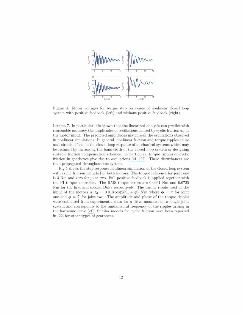
Lemma 7. In particular it is shown that the linearized analysis can predict withreasonable accuracy the amplitudes of oscillations caused by cyclic friction τd atthe motor input. The predicted amplitudes match well the oscillations observedin nonlinear simulations. In general, nonlinear friction and torque ripples causeundesirable effects in the closed loop response of mechanical systems which maybe reduced by increasing the bandwidth of the closed loop system or designingsuitable friction compensation schemes. In particular, torque ripples or cyclicfriction in gearboxes give rise to oscillations [21] [22]. These disturbances arethen propagated throughout the system.

Fig.5 shows the step response nonlinear simulation of the closed loop systemwith cyclic friction included in both motors. The torque reference for joint oneis 3 Nm and zero for joint two. Full positive feedback is applied together withthe PI torque controller. The RMS torque errors are 0.0961 Nm and 0.0725Nm for the first and second DoFs respectively. The torque ripple used at theinput of the motors is τd = 0.013 cos(2θm + φ) Nm where φ = π for jointone and φ = π

2 for joint two. The amplitude and phase of the torque rippleswere estimated from experimental data for a drive mounted on a single jointsystem and corresponds to the fundamental frequency of the ripples arising inthe harmonic drive [21]. Similar models for cyclic friction have been reportedin [22] for other types of gearboxes.

12

10−4

10−3

10−2

10−1

100

Mag

nitu

de (

abs)

10−2

10−1

100

101

102

103

−180

−90

0

90

Pha

se (

deg)

Bode Diagram

Frequency (Hz)

τd1

(cyclic friction 0.013333 Nm)

τd2

(cyclic friction 0.013333 Nm)

F=34.5 HzMag (abs) = 0.172

Figure 6: Bode plot of joint torque with torque ripple disturbance for the twoDoF system. The peak magnitude is about 35 Hz.

0 5 10 152.8

2.9

3

3.1

3.2

τL

1 (N

m)

0 5 10 15−20

−10

0

10

20

v m1 (

Vol

ts)

0 5 10 15−0.2

−0.1

0

0.1

0.2

τL

2 (N

m)

seconds0 5 10 15

−40

−20

0

20

40

v m2 (

Vol

ts)

seconds

Figure 5: Joint torque step response with torque ripple disturbance and thecorresponding control input for a two DoF system.

The bode plots in Fig.6 show how the disturbances τd affect the joint torque.The worst case is the resonance at 35 Hz while all other frequencies are atten-uated much further. Note that the peak amplitude in the bode plot predictsquite well the oscillation peaks in the nonlinear simulation shown in Fig.3. Thepower spectral density of the torque oscillation errors due to cyclic friction isshown in Fig.7. The figure clearly shows that peak values occur in the frequencyrange 30 − 40 Hz which is in the neighborhood of resonant peak in the bodeplot.

3.3.1 Resonance Compensation

There are several options to reduce the effect of torque ripples, for example usinglead or notch compensators in cascade with the PI controllers. For the nonlinearsimulation shown in Fig.8, a lead compensator GLC(s) = ( 628128 )

s+128s+628 is added

in cascade with the PI controller. The simulation clearly shows a substantialreduction in the peak amplitude of the oscillations to about 0.1. The RMS

13

0 20 40 60 80 1000

1

2

3

4

5

6

7x 10

−5

Hz

Pow

er/H

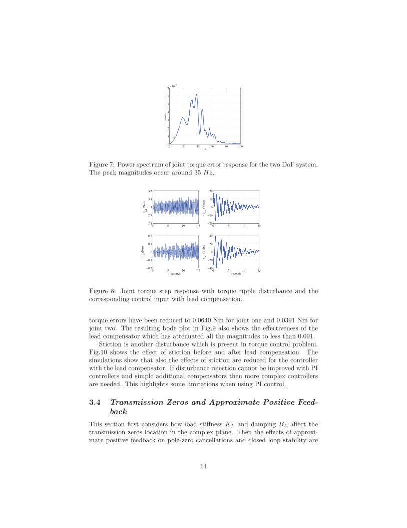
zFigure 7: Power spectrum of joint torque error response for the two DoF system.The peak magnitudes occur around 35 Hz.

0 5 10 152.8

2.9

3

3.1

3.2

τL

1 (N

m)

0 5 10 15−20

−10

0

10

20

v m1 (

Vol

ts)

0 5 10 15−0.2

−0.1

0

0.1

0.2

τL

2 (N

m)

seconds0 5 10 15

−40

−20

0

20

40

v m2 (

Vol

ts)

seconds

Figure 8: Joint torque step response with torque ripple disturbance and thecorresponding control input with lead compensation.

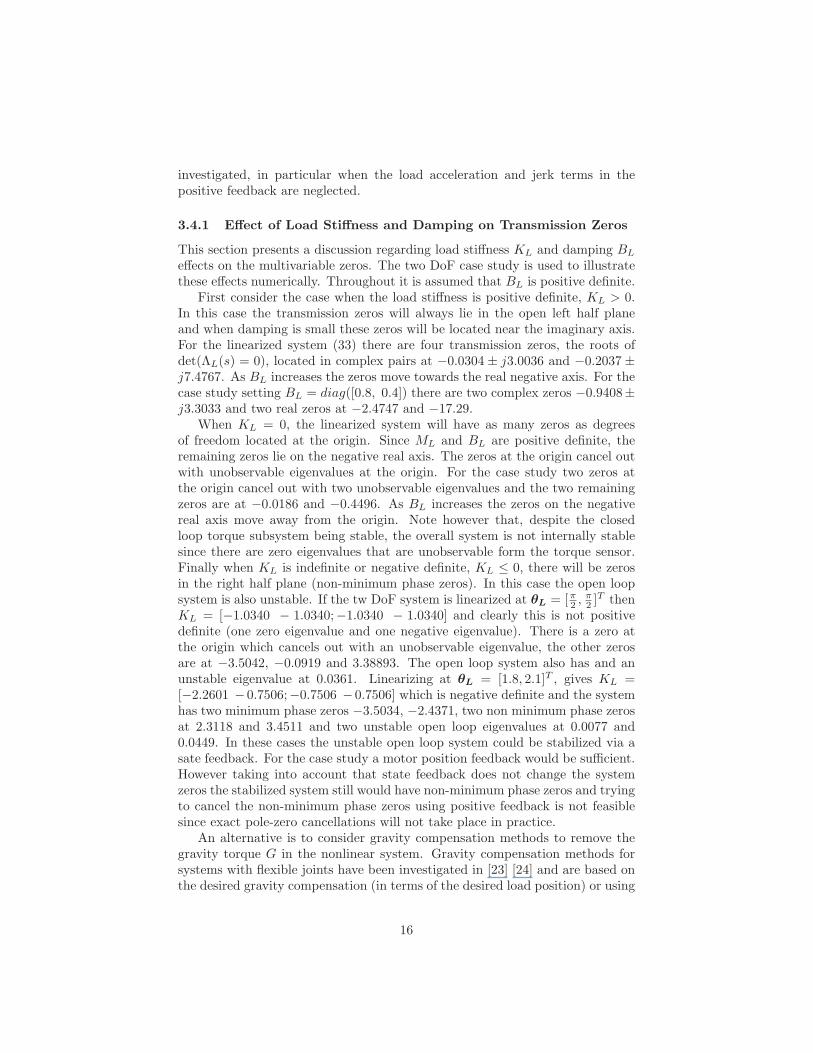
torque errors have been reduced to 0.0640 Nm for joint one and 0.0391 Nm forjoint two. The resulting bode plot in Fig.9 also shows the effectiveness of thelead compensator which has attenuated all the magnitudes to less than 0.091.

Stiction is another disturbance which is present in torque control problem.Fig.10 shows the effect of stiction before and after lead compensation. Thesimulations show that also the effects of stiction are reduced for the controllerwith the lead compensator. If disturbance rejection cannot be improved with PIcontrollers and simple additional compensators then more complex controllersare needed. This highlights some limitations when using PI control.

3.4 Transmission Zeros and Approximate Positive Feed-back

This section first considers how load stiffness KL and damping BL affect thetransmission zeros location in the complex plane. Then the effects of approxi-mate positive feedback on pole-zero cancellations and closed loop stability are

14

10−4

10−3

10−2

10−1

Mag

nitu

de (

abs)

10−2

10−1

100

101

102

103

−180

−90

0

90P

hase

(de

g)

Frequency (Hz)

τd1

(cyclic friction 0.013333 Nm)

τd2

(cyclic friction 0.013333 Nm)

F= 8.1 HzMag = 0.091

Figure 9: Bode plot of joint torque with ripple disturbance for the two DoFsystem with lead compensation.

0 5 10 152

3

4

seconds

τL

1 (N

m)

0 5 10 15−40

−20

0

20

40

seconds

v m1 (

Vol

ts)

0 5 10 15−1

0

1

seconds

τL

2 (N

m)

0 5 10 15−50

0

50

seconds

v m2 (

Vol

ts)

0 5 10 152

3

4

seconds

τL

1 (N

m)

0 5 10 15−40−20

02040

seconds

v m1 (

Vol

ts)

0 5 10 15−1

0

1

seconds

τL

2 (N

m)

0 5 10 15−50

0

50

seconds

v m2 (

Vol

ts)

C C

C C

U U

U U

Figure 10: Torque step responses of lead compensated (C) and uncompensated(U) system with cyclic friction and stiction.

15

investigated, in particular when the load acceleration and jerk terms in thepositive feedback are neglected.

3.4.1 Effect of Load Stiffness and Damping on Transmission Zeros

This section presents a discussion regarding load stiffness KL and damping BL

effects on the multivariable zeros. The two DoF case study is used to illustratethese effects numerically. Throughout it is assumed that BL is positive definite.

First consider the case when the load stiffness is positive definite, KL > 0.In this case the transmission zeros will always lie in the open left half planeand when damping is small these zeros will be located near the imaginary axis.For the linearized system (33) there are four transmission zeros, the roots ofdet(ΛL(s) = 0), located in complex pairs at −0.0304 ± j3.0036 and −0.2037 ±j7.4767. As BL increases the zeros move towards the real negative axis. For thecase study setting BL = diag([0.8, 0.4]) there are two complex zeros −0.9408±j3.3033 and two real zeros at −2.4747 and −17.29.

When KL = 0, the linearized system will have as many zeros as degreesof freedom located at the origin. Since ML and BL are positive definite, theremaining zeros lie on the negative real axis. The zeros at the origin cancel outwith unobservable eigenvalues at the origin. For the case study two zeros atthe origin cancel out with two unobservable eigenvalues and the two remainingzeros are at −0.0186 and −0.4496. As BL increases the zeros on the negativereal axis move away from the origin. Note however that, despite the closedloop torque subsystem being stable, the overall system is not internally stablesince there are zero eigenvalues that are unobservable form the torque sensor.Finally when KL is indefinite or negative definite, KL ≤ 0, there will be zerosin the right half plane (non-minimum phase zeros). In this case the open loopsystem is also unstable. If the tw DoF system is linearized at θL = [π2 ,

π2 ]

T thenKL = [−1.0340 − 1.0340;−1.0340 − 1.0340] and clearly this is not positivedefinite (one zero eigenvalue and one negative eigenvalue). There is a zero atthe origin which cancels out with an unobservable eigenvalue, the other zerosare at −3.5042, −0.0919 and 3.38893. The open loop system also has and anunstable eigenvalue at 0.0361. Linearizing at θL = [1.8, 2.1]T , gives KL =[−2.2601 −0.7506;−0.7506 −0.7506] which is negative definite and the systemhas two minimum phase zeros −3.5034, −2.4371, two non minimum phase zerosat 2.3118 and 3.4511 and two unstable open loop eigenvalues at 0.0077 and0.0449. In these cases the unstable open loop system could be stabilized via asate feedback. For the case study a motor position feedback would be sufficient.However taking into account that state feedback does not change the systemzeros the stabilized system still would have non-minimum phase zeros and tryingto cancel the non-minimum phase zeros using positive feedback is not feasiblesince exact pole-zero cancellations will not take place in practice.

An alternative is to consider gravity compensation methods to remove thegravity torque G in the nonlinear system. Gravity compensation methods forsystems with flexible joints have been investigated in [23] [24] and are based onthe desired gravity compensation (in terms of the desired load position) or using

16

−0.4 −0.35 −0.3 −0.25 −0.2 −0.15 −0.1 −0.05 0

−6

−4

−2

0

2

4

6

8

Real

Imag Transmission Zeros

(a) Zoom on the transmission zeros.

−100 −80 −60 −40 −20 0

−300

−200

−100

0

100

200

300

Real

Imag

(b) Overall view of the root locus.

Figure 11: Root locus plot as the positive feedback varies, α ε [0, 1], for the PIcontroller gain k0 = 2

a motor biased compensation. However these methods are only approximate anddo not completely remove the gravity torques. Methods employing the actualload position for gravity compensation could be used but these have not beenstudied in detail and at present we cannot ensure that this is a suitable approachin conjunction with the positive feedback scheme for torque control, particularlyfor systems that give rise KL being indefinite or negative definite. This questionis left open for future research. Therefore when KL ≤ 0 the positive feedbackcompensation does not seem to be a suitable strategy for torque control.

3.4.2 Effect of Approximate Positive Feedback on Stability

This section considers approximate implementations of the positive feedbackcompensation for the two DoF case study. In particular, we investigate theeffects on closed loop stability when ignoring terms involving load accelerationand jerk.

First consider the positive feedback in (23) and let α = αj = αa = αv, whereα takes values in the interval [0, 1]. In this analysis the acceleration and jerk arecomputed from equations (18)-(19) written in state feedback form. For α = 0there is no positive feedback applied while for α = 1 the full compensation isused. For intermediate values of α, a partial positive feedback compensation isimplemented. The closed loop poles are given by the roots of the characteristicpolynomial in Lemma 6. As α varies, Fig.11(a) and 11(b) show the root locus ofthe closed loop poles for the two DoF system and the PI controller gain k0 = 2in (34). The position of the transmission zeros are shown as circles and thepoles are shown as crosses. Fig.11(a) displays the root locus in the vicinity ofthe transmission zeros and for α = 1 four poles cancel the four zeros. Fig.11(b)shows an overall view of the root locus. From this analysis we conclude thatthe closed loop two DoF system with the PI controller remains stable for all αε [0, 1].Neglecting the jerk term :Consider the positive feedback (23) with αa = αv = 1 and αj = 0 so that

17

the term involving jerk is removed. Using Lemma 6 the effect of discarding jerkfeedback is investigated. For the two DoF case study, Fig.12(a) and 12(b) displaythe root locus plot around the transmission zeros without the jerk feedback termand varying the PI gain ko in the interval [0, 6]. In Fig.12(b) it can be seenthat the angle of departure from the pole is towards the unstable region but thepole is quickly drawn toward the transmission zero. In this case, ignoring thejerk term does not produce an unstable closed loop system. This result can alsobe verified for the nonlinear system via a simulation.

Unfortunately this conclusion does not hold in general and we next providean example showing that without jerk feedback instability can arise. For thetwo DoF system, KL > 0 and BL is very small. Now suppose that a motorwith a different and larger electrical time constant was chosen, for example ifthe inductance L was larger by a factor of ten. In this case varying the PI gainsko in the interval [0, 0.6] we arrive at a conditionally stable system 1. Stabilitywithout jerk feedback could be recovered if the damping BL were sufficientlylarge, for example if BL = diag[0.1, 0.1]). In summary, when KL > 0, there arecases in which jerk feedback cannot be discarded and Lemma 6 can be used toinvestigate this issue.

When the load stiffness KL = 0, numerous nonlinear simulations withoutjerk feedback have not shown stability problems. However a proof for thisconjecture is left as an open question. Recall that for KL = 0, the transmissionzeros lie on the real negative axis as opposed to the complex zeros presented insection 3.4.1. It seems that in this situation it is easier to compensate the effectof load motion without jerk feedback.

−0.2 −0.15 −0.1 −0.05 0

−8

−6

−4

−2

0

2

4

6

8

Real

Imag

Transmission Zeros

(a) Root locus near transmis-sion zeros.

−0.2 −0.15 −0.1 −0.05

7.42

7.44

7.46

7.48

7.5

7.52

7.54

Real

Imag

(b) Root locus near one zero.

Figure 12: Root locus plot of the approximate positive feedback near the trans-mission zeros, without jerk feedback and varying the PI torque controller gainko in the interval [0, 6]

Neglecting jerk Γj and acceleration Γa :Consider the positive feedback (23) with αv = 1 and αa = αj = 0 so that theterms involving acceleration and jerk are removed. Using Lemma 6 the effect ofdiscarding these terms is investigated. First consider the two DoF case study,when KL > 0 and BL is very small. In the root locus plot shown in Fig.13 it

1Conditional Stability: A conditionally stable system switches between stable an unstableoperation as the loop gain varies.

18

−0.2 0 0.2 0.4 0.6 0.8 1 1.21

2

3

4

5

6

7

8

Real

Imag

Figure 13: Root locus plot of the approximate positive feedback near transmis-sion zeros, without jerk and acceleration feedback and varying the PI torquecontroller gain ko ∈ [0, 6].

can be seen that the angles of departure from the poles are toward the unstableregion and the system is conditionally stable. Instability occurs for PI gains koin the intervals (0.00073, 7.5196) and ko > 12.53. Stability can be restored byfurther increasing the gain ko but then performance becomes quite oscillatorybecause other poles get close to the imaginary axis. When KL > 0 and BL issufficiently large, for example if BL = diag{0.8, 0.4}, then the close loop systemwithout acceleration and jerk feedback remains stable as shown in Fig.14(a).In summary, when KL > 0, there are cases in which acceleration and/or jerkfeedback cannot be discarded. This can be investigated using Lemma 6. Finally,when KL = 0 the system without acceleration and jerk feedback appears toremain stable. This conjecture is left open for future research.

−180 −160 −140 −120 −100 −80 −60 −40 −20 0

−400

−300

−200

−100

0

100

200

300

400

Real

Imag

(a) Overall root locus.

−18 −16 −14 −12 −10 −8 −6 −4 −2 0

−10

−5

0

5

10

Real

Imag

(b) Zoomed area near the ori-gin.

Figure 14: Root locus plot of the approximate positive feedback without jerkand acceleration feedback for larger damping BL and varying the PI torquecontroller gain ko ∈ [0, 6].

4 Experimental Results

The proposed positive feedback and lead compensation was implemented onthe robotic prototype leg presented in [14], and shown in Fig.15 to verify thetheoretical results. A 3.6 kg weight was attached at the leg end-effector (center

19

of mass at 0.42 m from the center of rotation including the mass of the lower leg)to increase the gravity load and permit a reasonable torque step magnitude. Theprototype robotic leg used has two actuators (M1 and M2) which both move theknee joint while the hip is un-actuated. In this experiment the second actuatorM2 which applies assistive torque at the knee using a bungee cord was removedand only the main knee motor M1 was used for the experimental verification.Moreover, the hip joint was mechanically locked and the leg was tested whilefixed above the ground on the supporting frame. In the experiments a torquestep of 3 Nm was applied and the results are presented as follows. The torquesignal is measured using two 19 bit encoders measuring the deflection of a torsionbar with known stiffness (930 Nm

rad ), connected between the gearbox output andthe link output. The estimated value of joint damping BL is 1.5 for the leg.Note that this value of BL is much larger than the joint damping used in the

simulation study presented in section 3. The PI controller Gc(s) = 2(s+10)s

was designed to have 46 Hz closed loop bandwidth with full positive feedback.The closed loop system also remains stable for the same PI controller withoutpositive feedback compensation but the closed loop bandwidth is substantiallyreduced to 0.7 Hz. The velocity is obtained using a 3rd order Butterworth filterwith cut-off frequency of 50 Hz and the acceleration and jerk are obtained withfirst order differentiation of the velocity and acceleration respectively.

Fig.16 compares the system’s torque step response in four cases. The steptorque reference (τr) is applied at t = 0.4 sec. First, part (a) in Fig. 16 showsthe closed loop step response without positive feedback. Second, in part (b) thesame PI controller is used with positive velocity feedback Γv = 6.909329. Third,part (c) the PI controller is used with positive velocity and acceleration feedbackΓa = 0.054354. Finally, in part (d) the same PI controller is used with fullpositive feedback proposed in Lemma 2 with positive velocity (Γv), acceleration(Γa) and jerk feedback Γj = 3.975e − 5. The bandwidth of the torque controlsystem with the velocity feedback increases to 46 Hz. As mentioned, sinceBL = 1.5 is large we can ignore the acceleration and jerk feedback terms withoutcausing instability or degrading closed loop performance.

When using the positive feedback compensation (see Fig.16) the torque set-tles at the desired value but a 15-20 Hz ripple can be observed which is due tothe harmonic drive gearbox friction. This frequency range is shown in the powerspectral density graph in Fig. 17. The lead compensator GLC =

(750128

)s+128s+750

is designed to improve disturbance attenuation of the torque ripples and tran-sient response of the torque control. GLC is placed in cascade with the outputof the PI controller. Fig.18 depicts the system’s torque step response in fourcases. The power spectral density plot of the lead compensated torque responseis shown in Fig.19. Clearly the magnitude of the oscillations around 15-20 Hzare considerably reduced by 50%.

20

Figure 15: The prototype robotic leg used in the experiments.

0 0.5 1 1.5 2−1

0

1

2

3

4

5

6

t (sec)

Nm

(a) PI

τ

r

τL

0 0.5 1 1.5 2−1

0

1

2

3

4

5

6

t (sec)

Nm

(b) PI, Γv

τ

r

τL

0 0.5 1 1.5 2−1

0

1

2

3

4

5

6

t (sec)

Nm

(c) PI, Γv, Γ

a

τ

r

τL

0 0.5 1 1.5 2−1

0

1

2

3

4

5

6

t (sec)

Nm

(d) PI, Γv, Γ

a, Γ

j

τ

r

τL

Figure 16: The experimental results of applying the positive feedback of theprototype leg. Torque reference and torque response are shown with dashed,solid lines, respectively. Parts (a), (b), (c) and (d) show the PI control, PIcontrol with velocity compensation, PI control with velocity and accelerationcompensation and PI control with velocity, acceleration and jerk compensation,respectively.

21

0 10 20 30 40 50 600

0.005

0.01

0.015

0.02

0.025

0.03

0.035

0.04

Hz

Pow

er/H

z

Figure 17: Spectral density plot of the uncompensated (without notch compen-sation) torque response.

0 0.5 1 1.5 2−1

0

1

2

3

4

5

6

t (sec)

Nm

(a) PI

τ

r

τL

0 0.5 1 1.5 2−1

0

1

2

3

4

5

6

t (sec)

Nm

(b) PI, Γv, Lead

τ

r

τL

0 0.5 1 1.5 2−1

0

1

2

3

4

5

6

t (sec)

Nm

(c) PI, Γv, Γ

a, Lead

τ

r

τL

0 0.5 1 1.5 2−1

0

1

2

3

4

5

6

t (sec)

Nm

(d) PI, Γv, Γ

a, Γ

j, Lead

τ

r

τL

Figure 18: The experimental results of applying the positive feedback withlead compensation of the prototype leg. Torque reference and torque responseare shown with dashed, solid lines, respectively. Parts (a), (b), (c) and (d)show the PI control, PI control with velocity and lead compensation, PI controlwith velocity, acceleration and lead compensation and PI control with velocity,acceleration, jerk and lead compensation, respectively.

0 10 20 30 40 50 600

0.005

0.01

0.015

0.02

0.025

0.03

0.035

0.04

Hz

Pow

er/H

z

Figure 19: Spectral density plot of the lead compensated torque response.

22

5 Conclusions

This paper provides a detailed study regarding the use of positive feedback toimprove torque control in flexible joint robots driven by electrical actuators. It isshown that torque control bandwidth limitations depend on the load dynamicsand a positive feedback scheme can be obtained to improve torque tracking forrobots with electrical actuators. A two DoF nonlinear system is used as anexample to illustrate torque tracking improvements that can be achieved withpositive feedback and simple PI controllers. Approximate positive feedbackimplementations are also considered and closed loop stability is analyzed usingroot locus methods. Simulations and experimental results for a prototype robotare shown to confirm the theoretical results.

6 MIMO Transmission Zeros

The linearized system equations can be written in matrix form

W (s)

⎡⎣ i

θm

θL

⎤⎦ = B vm (35)

where,

W (s) =

⎡⎣ Ls+R Kω s 0

−Kt Λ1(s) −N−1KH

0 −KHN−1 ΛL(s) +KH

⎤⎦ , B =

⎡⎣ I

00

⎤⎦ (36)

Λ1(s) = Λm(s)+N−1KHN−1, Λm(s) = Jms2+Bms, ΛL(s) = MLs2+BLs+KL

and KL includes the linearized gravity torques. The system matrix P (s) isdefined as

P (s) =

[W (s) −BC 0

](37)

The system zeros are the values s0 where P (s0) looses rank, that is

rank(P (s0)) < n+min(rank(C), rank(B)

where n is twice the number of DoF. The system zeros include the transmissionzeros and input/output decoupling zeros. When the system is controllable andobservable there are no input/output decoupling zeros. In the transfer functionmatrix, input/output decoupling zeros cancel out with uncontrollable and/orunobservable poles.

We need to show that P (s) looses rank iff det(MLs2 + BLs + KL) = 0.

To accomplish this we carry out a series of elementary transformation of thesystem matrix P (s). These transformations amount to post-multiply and/orpre-multiply P (s0) by a series of unimodular matrices. A unimodular matrix isa square polynomial matrix that has a constant (non-zero) determinant. The

23

inverse of a unimodular matrix is also a unimodular matrix.Let P (s) = Q1(s)P (s)Q2(s),

Q1(s) =

⎡⎢⎢⎣

I 0 0 00 I 0 00 0 I I0 0 0 K−1

H

⎤⎥⎥⎦ (38)

andQ2(s) =

⎡⎢⎢⎣

−K−1t 0 0 00 I 0 00 0 I 0

−(Ls+R)K−1t Kωs 0 −I

⎤⎥⎥⎦

⎡⎢⎢⎣

I −Λ1(s)N −Λ1(s)N +N−1KH 00 N N 00 0 I 00 0 0 I

⎤⎥⎥⎦ (39)

Then

P (s) =

⎡⎢⎢⎣

0 0 0 II 0 0 00 0 ΛL(s) 00 I 0 0

⎤⎥⎥⎦ (40)

It is clear that Q1(s) and Q2(s) are unimodular matrices and therefore P (s)and P (s) are equivalent. It is also evident that P (s) looses rank iff ΛL(s) loosesrank and this in turn is equivalent to the condition det(ΛL(s)) = 0.

7 Proof of Lemma 2

The plant output torque is given by

y = C

⎡⎣ i

θmθL

⎤⎦ (41)

where C = [0 KHN−1 −KH ]. Converting (36) in terms of torque τL gives

W (s)

⎡⎣ i

θm

θL

⎤⎦ = W (s)

⎡⎣ I 0 0

0 NK−1H N

0 0 I

⎤⎦⎡⎣ i

τL

θL

⎤⎦ = B vm (42)

Let,vm = F (s)θL + vr, (43)

Then (35), (36), (42) and (43) yield

⎡⎣ (Ls+R) (KωNK−1

H s) (KωNs− F (s))−Kt (Λ1(s)NK−1

H ) (Λ1(s)N −N−1KH)0 −I ΛL(s)

⎤⎦⎡⎣ i

τL

θL

⎤⎦ = B vr (44)

From (44) solving for the motor current i, substituting in the equation for thetorque τL and pre-multiplying by (Ls+R)K−1

t yields

[((Ls+R)K−1

t Λ1(s) +Kωs)NK−1H (Ls+R)K−1

t Λm(s)N +KωNs− F (s)−I ΛL(s)

] [τL

θL

]=

[vr

0

](45)

8 Block Companion Matrix

Consider a polynomial matrix P (s) = Pnsn + Pn−1s

n−1 + ...+ P1s+ P0 wherePi and p ×p constant matrices and Pn is invertible. A block companion matrix

24

representation of P (s) is

A =

⎡⎢⎢⎢⎢⎢⎣

0 I 0 0 0 00 0 I 0 0 0...

......

......

...0 0 0 0 0 I−P−1

n P0 −P−1n P1 −P−1

n P2 · · · −P−1n Pn−2 −P−1

n Pn−1

⎤⎥⎥⎥⎥⎥⎦

where 0 and I are p × p zero and identity matrices respectively.

References

[1] H Vallery, R Ekkelenkamp, H Van Der Kooij, and M Buss, Passive and ac-curate torque control of series elastic actuators, in IEEE/RSJ InternationalConference on Intelligent Robots and Systems, IROS, pp. 3534-3538, 2007.

[2] G.A. Pratt, M.M. Williamson, Series elastic actuators, in IEEE/RSJ In-ternational Conference on Intelligent Robots and Systems, ’Human RobotInteraction and Cooperative Robots’, vol.1, pp. 399-406, 5-9 Aug 1995.

[3] G.A. Pratt and M.M. Williamson, Stiffness Isn’t Everything, Fourth Inter-national Symposium on Experimental Robotics, 1995.

[4] S. Dyke, B. Spencer Jr., P. Quast, and M. Sain, Role of control-structureinteraction in protective system design, Journal of Engineering Mechanics,ASCE, vol. 121 no.2, pp. 322-38, 1995.

[5] A. Alleyne, R. Liu and H. Wright, On the limitations of force trackingcontrol for hydraulic active suspensions, in Proceedings of the AmericanControl Conference, Philadelphia, Pennsylvania, USA, pp. 43-47, 1999.

[6] J. Dimig, C. Shield, C. French, F. Bailey, and A. Clark. Effective forcetesting: A method of seismic simulation for structural testing, Journal ofStructural Engineering-Asce, vol. 125, no.9, pp. 1028-1037, 1999.

[7] C. K. Shield, C. W. French, and J. Timm, Development and implementationof the effective force testing method for seismic simulation of large-scalestructures, Philosophical Transactions of the Royal Society of London Seriesa-Mathematical Physical and Engineering Sciences, vol. 359 no. 1786, pp.1911-1929, 2001.

[8] M. Hashimoto, and Y. Kiyosawa, Experimental study on torque controlusing Harmonic Drive built-in torque sensors, Journal of Robotic Systems,vol. 15, no. 8, pp.435–445, 1998.

[9] T. Boaventura, M. Focchi, M. Frigerio, J. Buchli, C. Semini, G. A.Medrano-Cerda, D. G. Caldwell, On the role of load motion compensa-tion in high-performance force control, in IEEE International Conferenceon Intelligent Robots and Systems (IROS), Vilamoura, Algarve, Portugal,pp. 4066-4071, 2012.

25

[10] C. Semini, N. G. Tsagarakis, E. Guglielmino, M. Focchi, F. Cannella, andD. G. Caldwell, Design of HyQ - a hydraulically and electrically actuatedquadruped robot, IMechE Part I: J. of Systems and Control Engineering,vol. 225, no. 6, pp. 831-849, 2011.

[11] F. Aghili, M. Buehler, and J. M. Hollerbach, Motion Control Systems withH∞ Positive Joint Torque Feedback, IEEE Trans. On Control SystemsTechnology, vol. 9, no. 5, pp. 685-695, Sept, 2001.

[12] Je Sung Yeon; Jong Hyeon Park, Practical robust control for flexible jointrobot manipulators, in Proc. of IEEE International Conference on Roboticsand Automation, pp. 3377-3382, 19-23 May, 2008.

[13] G. Hirzinger, A. Albu-Schaeffer, M. Haehnle, I. Schaefer, and N. Sporer,On a new generation of torque controlled light-weight robots, in ProceedingsIEEE International Conference on Robotics and Automation, volume 4, pp.3356-3363, 2001.

[14] N.G. Tsagarakis, S. Morfey, H. Dallali, G.A. Medrano-Cerda, and D.G.Caldwell, An Asymmetric Compliant Antagonistic Joint Design for HighPerformance Mobility, in Proc. of IEEE/RSJ International Conference onIntelligent Robots and Systems (IROS), pp. 5512-5517, November 3-7,2013, Tokyo, Japan.

[15] S. Skogestad and I. Postlethwaite I, Multivariable feedback control: analysisand design 2nd ed. Wiley-Blackwell, 2007.

[16] B. A. Levant, Higher-Order Sliding Modes, Differentiation and Output-Feedback Control, Int. J. of Control, vol. 76, nos 9/10, pp. 924-941, 2003.

[17] C. A. Levant and M. Livne, Exact Differentiation of Signals with Un-bounded Higher Order Derivatives, IEEE Trans on Automatic Control,vol. 57, no. 4, pp. 1076-1080, April 2012.

[18] E. S. Ibrir, Linear Time-Derivative Trackers, Automatica vol.40, pp. 397-405, 2004.

[19] M. Smaoui, X. Brun and D. Thomasset, High-order sliding mode for anelectropneumatic system: A robust differentiatorcontroller design, Int. J.Robust Nonlinear Control, vol. 18, 2008, pp. 481501.

[20] Y.X. Su, C.H. Zheng, Dong. Sun, and BY. Duan, A simple nonlinear ve-locity estimator for high-performance motion control, IEEE Transactionson Industrial Electronics, vol. 52, no. 4, pp. 1161-1169, 2005.

[21] T. D. Tuttle and W. A. Seering W. A nonlinear model of a harmonic drivegear transmission, IEEE Trans on Robotics and Automation, vol. 12, 1996,pp.368-374.

26

[22] E. Garcia, P. Gonzalez de Santos and C. Canudas De Wit, Velocity depen-dence in the cyclic friction arising with gears, Int. J. of Robotics Research,vol.21, 2002. pp.761-771.

[23] P. Tomei, A Simple PD Controller for Robots with Elastic Joints, IEEETrans on Automatic Control, vol. 36, 1991, pp.1208-1213.

[24] A. De Luca, B. Siciliano, and L. Zollo, PD control with on-line gravitycompensation for robots with elastic joints: Theory and experiments. Au-tomatica, vol.41, 2005, pp.1809-1819.

27