FONDATION POUR LES ETUDES ET RECHERCHES SUR LE DEVELOPPEMENT INTERNATIONAL

Measuring macroeconomic volatility

Applications to export revenue data, 1970-2005.

by

Joël Cariolle

Working paper n°I14

“Innovative indicators” series

March 2012

Page | 1

Measuring macroeconomic volatility: applications to

export revenue data, 1970-2005.

Joel Cariolle†

Summary

The literature on macroeconomic volatility covers an extremely wide field, as evidenced by the

very broad spectrum of indicators used to grasp it as a phenomenon. In general there seems to

be little discussion about the choice of indicator for macroeconomic volatility, on the grounds

that the different methods, based on stationary series, give rise to scores which are closely

correlated. Although these methods may converge when analysing only the average magnitude

of distribution around a reference value, however, they diverge significantly when one examines

either asymmetry or kurtosis (instances of extreme deviation). This article reviews the existing

literature and sets out the principal methods used for calculating volatility. These methods are

compared and their properties analysed based on export revenue data for 134 countries from

1970 to 2005. In particular, a distinction is drawn between measurements of the magnitude of

volatility and measurements of asymmetry and the incidence of extreme deviations.

† Foundation for International Development Study and Research, 63 Bvd François Mitterrand, 63000 Clermont-

Ferrand, France. I would like to thank Patrick Guillaumont, Michaël Goujon, Jean-Louis Combes and Laurent Wagner

for their practical support and comments.

Page | 2

TABLE OF CONTENTS

1. Introduction ........................................................................................................................................... 4

1.1. Macroeconomic volatility and development. ................................................................................... 4

The costs of volatility .............................................................................................................................................................. 4

Internal economic conditions resulting in greater vulnerability to economic volatility. .............................. 5

The origins of macroeconomic volatility ........................................................................................................................... 7

1.2. Measures of economic volatility: a variety of indicators. ............................................................. 8

Economic volatility as the standard deviation of the growth rate of a variable .............................................. 9

Economic volatility as the standard deviation of the residual of an econometric regression ..................... 9

Economic volatility as the standard deviation of the cycle isolated by a statistical filter ......................... 10

2. The question of reference values .................................................................................................. 12

2.1. Breakdown of economic series ............................................................................................................ 13

Observation of series behaviour ...................................................................................................................................... 13

Theoretical breakdown of series ..................................................................................................................................... 14

Volatility as a measure of variability, risk or uncertainty? ................................................................................... 15

2.2. Parametric approach ................................................................................................................................ 16

Estimate based on a linear deterministic trend ........................................................................................................ 16

Estimate based on a mixed trend .................................................................................................................................... 18

Estimate based on a rolling mixed trend ..................................................................................................................... 20

2.3. Filtering approach .................................................................................................................................... 22

3. Calculating deviation from the trend .......................................................................................... 26

3.1. Calculation period for volatility .......................................................................................................... 26

3.2. The magnitude of volatility .................................................................................................................. 27

3.3. The asymmetry of volatility .................................................................................................................. 30

3.4. Frequency of extreme deviations ........................................................................................................ 33

Conclusion .................................................................................................................................................... 38

Bibliography ................................................................................................................................................. 39

Appendices ................................................................................................................................................... 43

FIGURES

Figure 1. Export series and spectrum densities for South Korea, Argentina, Venezuela, Kenya, Ivory Coast and Burundi. ................................................................................................................................... 14

Figure 2. Change in export revenues, simple linear trend. ...................................................................................... 17

Figure 3. Residual of linear trend ............................................................................................................................................ 17

Figure 4. Change in export revenues, mixed trend. ..................................................................................................... 19

Figure 5. Correlogram of residuals, mixed trend .......................................................................................................... 20

Figure 6. Rolling mixed trend, comparative change and correlogram of residuals, Argentina. ........... 21

Figure 7. Global and rolling mixed trends, comparative change and correlogram of residuals, Burundi. ....................................................................................................................................................................... 22

Figure 8. Export revenues smoothed by HP filter ........................................................................................................ 25

Figure 9. Magnitude of volatility – deviations (as % of trend) for the last five years around a mixed trend ................................................................................................................................................................ 28

Figure 10. Graphical illustration of correlations between magnitude of volatility indicators. .............. 29

Page | 3

Figure 11 Graphical illustration of a positive and negative asymmetric distribution of identical magnitude. ................................................................................................................................................................. 30

Figure 12. Correlation between magnitude and asymmetry of volatility indicators, by reference value. ............................................................................................................................................................................. 32

Figure 13. Graphic representation of the degree of flattening of a distribution ............................................ 33

Figure 14. Graphical illustration of correlations between magnitude and kurtosis of volatility indicators, by reference value ........................................................................................................................... 35

Figure 15. Correlation between asymmetry and kurtosis of volatility indicators, by reference value .............................................................................................................................................................................. 37

TABLES

Table 1: Specification and unit root test on panel data .............................................................................................. 19

Table 2. Correlation between magnitude of volatility indicators. ........................................................................ 28

Table 3. Descriptive statistics of magnitude of volatility indicators (%). .......................................................... 29

Table 4. Correlations of coefficients of asymmetry calculated over the period 1982-2005. ...................... 31

Table 5. Descriptive statistics for kurtosis calculated for the period 1982-2005. ........................................... 34

Table 6. Correlations in kurtosis calculated over the period 1982-2005 ............................................................. 34

Table 7. Correlations between kurtosis and coefficient of asymmetry for each reference value, 1982-2005. .......................................................................................................................................................................................... 36

APPENDICES

Appendix A.1 Overview of indicators of volatility and their application in the literature. .................... 44

Appendix A.2. Mixed trends and correlogram of residuals .................................................................................... 46

Appendix A.3. Correlogram of export revenue cycles smoothed by the HP filter ...................................... 48

Appendix A.4 Comparative evolution of deviations (in % of trend values) ................................................... 49

Page | 4

1. Introduction

The numerous global economic crises of the 20th century have made macroeconomic volatility a key

issue in analysing the determinants of economic growth. The multiplicity of ways in which it affects

the long-term growth potential of economies, its diverse causes and the array of methods by which

it is measured, make economic volatility a complex and multidimensional phenomenon. We

therefore consider the term “volatility” as a generic term, combining all the techniques available for

measuring economic fluctuations.

1.1. Macroeconomic volatility and development.

The literature provides an extensive analysis of the costs and consequences of macroeconomic

volatility. Although the positive relationship between risk and capital yield may, under certain

conditions, explain a positive relationship between economic volatility and growth, most research

agrees that this phenomenon has a negative impact on long-term growth and well-being. Indeed,

over the long term, volatility contributes to a reduction in levels of consumption, investment and

factor productivity, to an increase in the volatility and unpredictability of economic policy, and to

deterioration in the institutional environment. The effects on performance are even more marked in

developing countries, which are often subjected to more significant external shocks but which do

not enjoy the internal conditions that would allow them to absorb them more easily. Hnatkovska

and Loayza (2005), Aizenman and Pinto (2005) and Loayza et al (2007) offer an exhaustive overview

of the consequences of macroeconomic volatility and the factors that cause it.

The costs of volatility

Macroeconomic volatility is a major obstacle to growth. According to estimates produced by

Hnatkovska and Loayza (2005), based on a sample of 79 countries, increasing the average value of

volatility by the value of its standard deviation results in an average loss of 1.3 points for growth in

GDP over the period 1960-2000, and 2.2 points for the decade 1990-2000. Volatility can, indeed, act

as an obstacle to the key factors in economic and social development.

An early series of research articles examined the impact of macroeconomic volatility on growth from

the point of view of investment or production factor productivity. Dawe (1996) analyses the effect of

volatility in exports on investment and growth. He finds both a positive effect of volatility on

investment through an increase in precautionary savings, and a negative effect on growth through

an allocation of capital to sectors with lower yields. Dehn (2000), on the other hand, identifies a

significant and negative impact of shocks in the price of raw materials on investment in developing

countries. Guillaumont, Guillaumont-Jeanneney, and Brun (1999) highlight a negative effect of

volatility in the rate of investment on growth, based on a decline in average productivity. In a

similar area, Koren and Tenreyro (2006) empirically test a theoretical model where development is

accompanied by increased diversification of inputs into the production system, thus reducing the

effect of volatility in world prices on production factor productivity and therefore on growth.

Finally, Combes and Guillaumont (2002) show that volatility in relation to terms of trade has a

Page | 5

negative impact on the growth rate of capital productivity. Macroeconomic volatility therefore

seems to be an obstacle to economic growth insofar as it discourages investment decisions, has a

negative effect on factor productivity and diverts capital from the most productive sectors.

Other studies analyse the impact of macroeconomic volatility on growth and well-being through its

effect on the quality of economic policy. Easterly et al (1993) show that positive shocks in relation to

terms of trade influence the long-term growth path of economies, in part through an improvement

in economic policy. Ramey and Ramey (1995) show that the unpredictability of economic policy

caused by volatility in growth rates has a negative effect on the average growth rate of the economy.

Guillaumont and Combes (2002) show that vulnerability to volatility in global prices has a negative

effect on the quality of economic policy and growth. To take two other examples, both Fatas and

Mihov (2006, 2007) and Afonso and Furceri (2010) have emphasised the negative impact of

variability in budget policy on growth in both OECD countries and developing nations.

The negative effect of macroeconomic volatility on growth and well-being, based on volatility in

public and private consumption, has also been examined in a number of studies. Aizenman and

Pinto (2005) and Wolf (2005) point out that in the case of imperfect financial markets, the State and

individual households are unable to protect themselves fully against risks which affect their revenue

and adjust their consumption to the vagaries of economic activity. The result is that volatility driven

by external factors, for example in relation to terms of trade, generates internal volatility in relation

to consumption, particularly in developing countries (Aguiar and Gopinath, 2007; Loayza et al,

2007).

Economic policy and consumption therefore appear to be internal channels by which

macroeconomic volatility is transmitted and may even be magnified, with a concomitant negative

effect on growth and development.

Internal economic conditions resulting in greater vulnerability to economic volatility.

One positive effect of volatility on growth has already been mentioned (Imbs, 2007; Rancière et al,

2008; Hnatkovska and Loayza, 2005). This can be explained primarily by the positive correlation

between risk and return on investment projects. Hnatkovska and Loayza (2005) suggest, however,

that a positive effect of this kind is dependent on the existence of risk-sharing mechanisms and

respect for rights of ownership, which are in turn supported by a well-developed financial system

and high-quality institutions. A country’s vulnerability to macroeconomic volatility is therefore

driven by a number of handicaps, which are either structural or depend on the level of economic

development. These factors explain why, in general terms, developing countries are more

vulnerable to macroeconomic volatility. Developing countries are more exposed to shocks, and do

not always have the mechanisms or internal conditions in place to enable them to absorb them. The

size of the population, the degree of diversification of the economy and the capacity for operating a

countercyclical economic policy, the existence of well-developed financial institutions and

institutional quality are therefore determining factors in the impact of volatility on growth.

The literature on economic vulnerability has made a significant contribution to our understanding

Page | 6

of the internal and external conditions of vulnerability to shocks (Guillaumont, 2007, 2009a, 2009b,

2010; Cariolle, 2011; Loayza and Raddatz, 2007; Combes and Guillaumont, 2002). The research

carried out distinguishes structural factors in relation to vulnerability from more transitory factors

linked to economic policy (or “resilience”). As far as structural factors are concerned, a distinction is

drawn between the magnitude and frequency of shocks (commercial or natural) and exposure to

such shocks. Factors that affect exposure to shocks (such as the size of the population, the degree of

economic diversification, distance from global markets and geographical isolation) increase the

propensity of economies to suffer shocks and the negative impact of such shocks on growth. A

recent study by Malik and Temple (2009), on the structural determinants of volatility in relation to

growth, suggests a negative relationship between access to global markets and macroeconomic

volatility. According to the authors, countries which are isolated from global markets tend to lack

diversity in terms of exports and experience greater volatility in relation to GDP. As to the resilience

of particular countries, although this is to some extent dependent on structural factors, it is linked

primarily to economic policy and institutions. As a result, development strategies with a focus on

foreign trade, the procyclicality and countercyclicality of economic policy and the quality of

governance and democratic institutions (Rodrik, 1998; 2000) can determine both the magnitude of

volatility experienced by countries and its effect on their development.

The contribution made by foreign trade to macroeconomic volatility is one of the themes most

commonly addressed in the literature. Whilst the role played by openness to trade has not been

clearly established (Combes and Guillaumont, 2002), several pieces of research have examined the

relationship between a country’s degree of specialisation, its level of development and

macroeconomic volatility. Di Giovanni and Levchenko (2010) study the extent to which openness to

trade can result in a specialisation of export sectors which are highly exposed to external shocks,

and thus to increased economic volatility. They show that countries with a low or moderate

comparative advantage in high-risk export sectors diversify their economy in order to attenuate the

risk affecting their export revenues. Conversely, countries with a very high level of comparative

advantage in these sectors tend to specialise in them, and are thus more exposed to volatility in

relation to terms of trade, exports and GDP growth per head. Similarly, Koren and Tenreyro (2006,

2007) show that poor countries specialise in a limited number of sectors, with relatively simple

production technologies and a limited range of inputs, and are therefore more vulnerable to shocks

in global prices. Development is therefore supported by diversification into sectors based on more

complex technologies, using a wider variety of inputs, and with less exposure to macroeconomic

volatility. Van der Ploeg and Poelhekke (2009) find that growth volatility, driven by volatility in

global raw materials prices, is the main determinant of the “natural resource curse”. Having

controlled for growth volatility, they show that supplies of natural resources have a positive and

significant effect on economic growth. Development is thus generally accompanied by economic

diversification and by specialising in sectors which are less exposed to global volatility. Conversely,

the negative effect of a low level of economic diversification on development is assumed to be

dependent on a high level of exposure to volatility in global prices.

Page | 7

Other studies have examined the quality of institutions in attenuating or contributing to economic

volatility. Acemoglu et al (2003) showed that poor institutions result in poor governance, which in

turn contributes to macroeconomic volatility. Mobarak (2005) finds that democracy reduces

volatility through increased scrutiny by citizens of the management of economic policy. These

results reflect those found by Rodrik (2000), according to which democratic political structures

encourage political consensus around political responses to external shocks. Numerous research

articles have also examined the role of the development of financial markets in transmitting

macroeconomic volatility (Beck et al, 2006; Aghion et al, 2005; Aghion et al, 2004). In general,

financial development therefore tends to attenuate shocks, although it seems to be able to magnify

the effect of shocks of monetary origin on volatility in GDP (Beck et al, 2006). The quality of political,

economic and financial institutions therefore seems to be both a source and a vector of

macroeconomic volatility.

The origins of macroeconomic volatility

Another set of literature examines the sources of macroeconomic volatility. This research generally

draws a distinction between external forms of volatility (exports, global prices, terms of trade or

international interest rates) and internal forms (such as economic policy, agricultural production

and natural or climatic disasters). Similarly, it is possible to distinguish between exogenous sources

of macroeconomic volatility (related to international trade, agricultural production and natural

disasters) and endogenous sources (linked to volatility in economic policy or domestic socio-

political conditions). Finally, several studies draw a distinction between so-called “normal”

fluctuations and “crisis” fluctuations, the magnitude of which exceeds a particular threshold

(Rancière et al., 2008; Hnatkovska and Loayza, 2005).

The literature on the economic vulnerability of developing countries emphasises the significant

contribution made by the magnitude and frequency of external and natural shocks to the structural

vulnerability of developing countries (Guillaumont, 2007, 2009a, 2009b, 2010; Cariolle, 2011; Loayza

and Raddatz, 2007; Combes and Guillaumont, 2002). Research by Mauro and Becker (2006) identifies

the external shocks that cause growth shocks, such as a deterioration in relation to terms of trade

and a sudden halt to the movement of capital. Similarly, Raddatz (2007) examines the sources of

volatility in GDP in the Least Developed Countries. He sets out an analysis of the total and relative

contribution of external shocks to volatility in GDP based on a breakdown of GDP variance.

Raddatz shows that external shocks (terms of trade, price of primary products, LIBOR and

development aid) have only a marginal effect on the volatility of the growth rate of GDP, whilst

internal factors related to economic policy (level of public deficit, inflation and overvaluation of

exchange rates) make a significant contribution. These results confirm those of Fatas and Mihov

(2006, 2007), showing that economic volatility results in part from volatility in budget policy.

Finally, Hnatkovska and Loayza (2005) distinguish between the effect on growth of “normal”

fluctuations in GDP (positive or negative, repeated and on an average scale) and the effect of

“crises” measured by falls in GDP over a certain threshold. The simultaneous introduction of these

two volatility variables in their regressions shows the important and significant effect of a “crisis”

Page | 8

level of volatility on growth and the insignificant effect of “normal” volatility. The same

classification of volatility was used by Rancière et al (2008) and applied to the effect of a financial

“systemic risk” on growth. They find a positive relationship between financial crisis and growth,

which is explained by the leverage effect of companies’ level of indebtedness on their investments.

The literature on macroeconomic volatility therefore covers something of a wide field, showing the

significant interest in understanding it and its decisive role on economic performance in relation to

growth. As we will see below, however, there is a diverse range of methods available for measuring

volatility, although there has been no real discussion of the advantages and disadvantages of such

methods since the research carried out by Gelb (1979) and Tsui (1988).

1.2. Measures of economic volatility: a variety of indicators.

Common definitions of volatility often refer to the notion of disequilibrium. Measuring economic

volatility involves evaluating the deviation between the values of an economic variable and its

equilibrium value. This equilibrium value, or reference value, in turn refers to the existence of a

permanent state or trend. In statistical terms, economic volatility is traditionally measured by the

second (standard deviation) or sometimes a higher moment1 (Rancière et al, 2008), of the

distribution of a variable around its mean or a trend, which then represents the equilibrium value

(to which the variable tends to return quickly after deviating in response to a shock). It is frequent

for macroeconomic series (GDP, export revenues, final consumption) to be “non-stationary”, i.e.

they fluctuate around a trend which itself varies over time, or for shocks to make the variable

deviate from its previous tendency over the long term or permanently. It then becomes necessary to

use so-called “stationarisation” techniques in order to separate the permanent (or trend) component

from the transitory (or residual) component of the evolution of a series (see section 2.1). The

volatility indicators obtained using these techniques are intended to reflect the effects of the episodic

variations of an economic series around a reference value (mean, deterministic trend or variable

over time). Calculating volatility thus relies on two key questions: that of calculating a reference value – or the choice of a stationarisation method – and measuring fluctuations around said reference value.

A distinction can be drawn between two main families of volatility indicators: on the one hand,

those which measure the variability of an economic series, i.e. taking into account all of the transitory

variations of a statistical series, and on the other, those which measure economic uncertainty, or the

unpredictability of variations in total variability (Wolf, 2005). We set out below a review of the main

indicators of economic volatility as presented in the literature, noting how reference values and

fluctuations have been calculated by various authors. A summary table of these indicators can be

found in Appendix A.1.

1Asymmetry and kurtosis coefficients of financial values are often used as measures of risk in the financial sector. In

economics, only Rancière et al (2008) have, to our knowledge, incorporated the effects of economic volatility into their research.

Page | 9

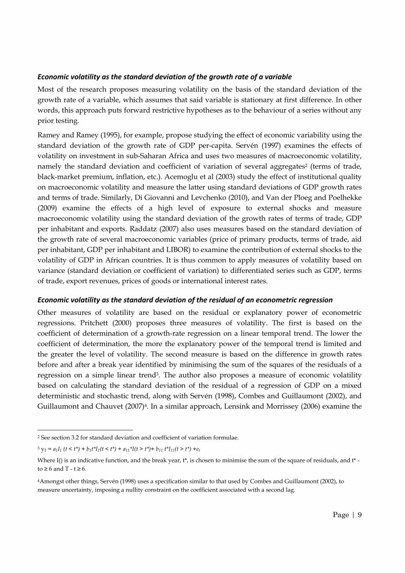
Economic volatility as the standard deviation of the growth rate of a variable

Most of the research proposes measuring volatility on the basis of the standard deviation of the

growth rate of a variable, which assumes that said variable is stationary at first difference. In other

words, this approach puts forward restrictive hypotheses as to the behaviour of a series without any

prior testing.

Ramey and Ramey (1995), for example, propose studying the effect of economic variability using the

standard deviation of the growth rate of GDP per-capita. Servén (1997) examines the effects of

volatility on investment in sub-Saharan Africa and uses two measures of macroeconomic volatility,

namely the standard deviation and coefficient of variation of several aggregates2 (terms of trade,

black-market premium, inflation, etc.). Acemoglu et al (2003) study the effect of institutional quality

on macroeconomic volatility and measure the latter using standard deviations of GDP growth rates

and terms of trade. Similarly, Di Giovanni and Levchenko (2010), and Van der Ploeg and Poelhekke

(2009) examine the effects of a high level of exposure to external shocks and measure

macroeconomic volatility using the standard deviation of the growth rates of terms of trade, GDP

per inhabitant and exports. Raddatz (2007) also uses measures based on the standard deviation of

the growth rate of several macroeconomic variables (price of primary products, terms of trade, aid

per inhabitant, GDP per inhabitant and LIBOR) to examine the contribution of external shocks to the

volatility of GDP in African countries. It is thus common to apply measures of volatility based on

variance (standard deviation or coefficient of variation) to differentiated series such as GDP, terms

of trade, export revenues, prices of goods or international interest rates.

Economic volatility as the standard deviation of the residual of an econometric regression

Other measures of volatility are based on the residual or explanatory power of econometric

regressions. Pritchett (2000) proposes three measures of volatility. The first is based on the

coefficient of determination of a growth-rate regression on a linear temporal trend. The lower the

coefficient of determination, the more the explanatory power of the temporal trend is limited and

the greater the level of volatility. The second measure is based on the difference in growth rates

before and after a break year identified by minimising the sum of the squares of the residuals of a

regression on a simple linear trend3. The author also proposes a measure of economic volatility

based on calculating the standard deviation of the residual of a regression of GDP on a mixed

deterministic and stochastic trend, along with Servén (1998), Combes and Guillaumont (2002), and

Guillaumont and Chauvet (2007)4. In a similar approach, Lensink and Morrissey (2006) examine the

2 See section 3.2 for standard deviation and coefficient of variation formulae.

3 y1 = a1I1 (t < t*) + b1t*I1(t < t*) + a11*I(t > t*)+ b11 t*I11(t > t*) +et

Where I() is an indicative function, and the break year, t*, is chosen to minimise the sum of the square of residuals, and t* -

to ≥ 6 and T - t ≥ 6.

4Amongst other things, Servén (1998) uses a specification similar to that used by Combes and Guillaumont (2002), to

measure uncertainty, imposing a nullity constraint on the coefficient associated with a second lag.

Page | 10

effect on economic growth of the volatility of Foreign Direct Investments (FDI) as measured by the

standard deviation of the residual of a regression of FDI on its three lags and a deterministic trend.

Other authors have tended to concentrate more on the effects of economic uncertainty on

investment and growth. Ramey and Ramey (1995) propose a measure of the uncertainty component

of volatility based on the standard deviation for prediction error against the growth rate (the

predicted value being obtained by a growth rate regression against a quadratic trend, linear trend,

two GDP lags and the initial values of the share of investment in GDP, population and human

capital)5. Servén (1998) and Dehn (2000) in turn examined the effect of economic uncertainty on

investment using several measures of uncertainty generated by price volatility in raw materials and

calculating the conditional standard deviation for prediction error for these series obtained using a

GARCH process (1,1).

Volatility measures based on the residual of econometric regressions thus have the merit of being

based on a less restrictive formalisation of the process underlying the change in the trend of

economic series. Nonetheless, it remains to be seen whether said formalisation allows proper series

stationarisation, and whether the interpretation of the residual is correct (uncertainty or

variability?).

Economic volatility as the standard deviation of the cycle isolated by a statistical filter

Finally, several studies have used the filtered value of a statistical series as a reference value. This

technique can be used to disaggregate a series into trend variations (long term) and cyclical

variations (short term). This type of volatility indicator is therefore based on cyclical or cycle

fluctuations. The filtering technique is different from the previous two methods insofar as it does

not formulate the behaviour of a series in advance (order of integration, difference-stationarity or

trend-stationarity) and filters series on the basis of their past and future behaviour. Section 2.3

examines this technique in more detail.

Dawe (1996) thus filters export series using a moving average based on five years, i.e. on [t-2;t+2],

and bases his volatility measurement on the average difference between the series observed and this

moving average. Other authors use the Hodrick-Prescott (Hodrick and Prescott, 1997) filter to

calculate their volatility indicator; they include Chauvet and Guillaumont (2007), who use the

standard deviation of the development aid cycle isolated using this filter (HP), i.e. the standard

deviation of the difference between the value smoothed by the filter and the observed value of their

aid variable. Becker and Mauro (2006) propose a shock variable based on the HP filter and identify

decreases in GDP as an event equating to a decline in filtered GDP of over 7%. Hnatkovska and

Loayza (2005) isolate the cyclical fluctuations in GDP series using the Baxter and King filter (1999)

and calculate their standard deviation. Finally, Afonso and Furceri (2010) use the standard deviation

of the cyclical component of public spending and tax revenues isolated using HP and Baxter-King

filters.

5The authors regress the following model for the whole of the sample for each country:

itinitialit

initialit

initialitititit KhumpopIyydummyttty εθδλγβϕαααα ++++++++++=∆ −− 21197419743

2210

Page | 11

The usual indicators of economic volatility can therefore be distinguished by the method used to

calculate the reference value selected. It is thus possible to draw a distinction between indicators

based on first-difference series variance, indicators based on the variance of the residual of a more

complex model of economic series, and those based on cyclical variance identified by applying

statistical filters. These distinctions become more blurred, however, with regard to the method used

to calculate deviations from the reference value, since the literature limits the analysis of volatility to

an analysis of the variance of volatility, i.e. the average magnitude of fluctuations6.

In the following section, we present an analysis of the various methods used for calculating a

reference value based on export data for the period 1970-2005 and illustrate the differences in the

analysis depending on the method used. In section three, we outline various ways of characterising

the fluctuations of a variable around a reference value, showing that it is possible to quantify

volatility not only by the average magnitude of economic fluctuations, but also in terms of their

asymmetry and the occurrence of extreme variations (or kurtosis).

6 Except for Rancière et al (2008).

Page | 12

2. The question of reference values

If volatility refers to the notion of disequilibrium, then it must be measured using stationary series.

Most economic aggregates, however, are not “naturally” stationary. It therefore becomes necessary

to calculate a reference value or trend value, around which series will be stationary, which in turn

means identifying the right method of stationarisation.

Or yt = µt + εt,, a non-stationary process with µt a non-constant term and εt the residual. Stationarising

yt consists of calculating or estimating the trend component µt so that the residual (or cycle) εt meets

the following conditions7:

(1) E(εt) = 0;

(2) V(εt)= σε2 < ∞ for all of t; and

(3) Cov(εt ; εt -k) = ρk.

These three conditions require the residual εt to have a zero mean (1), a variance (2) and a finite

autocovariance (3) independent of time. Volatility measures are based on the residual (or cycle) εt,,

which therefore reflects only transitory fluctuations. If the series is poorly stationarised, variations

which are attributable to a long-term (or permanent) change in yt may be included in the residual,

thus breaching conditions (1), (2), and (3). The volatility measures based on them would therefore be

incorrect, because they do not correspond with the definition given to them. Stationarisation is a

prerequisite condition for calculating volatility based on non-stationary level series. Calculating a

reference value is therefore a fundamental step, since it results in identifying and isolating the trend

or permanent component in the change of an economic variable, from its transitory or stationary

component (Dehn, 2000; Hnatkovska, 2005). To understand this issue in more detail, we first

examine the theoretical breakdown of change in statistical series. We then present the principles and

properties of the usual methods for calculating reference values, which we apply to export data.

We illustrate our analysis using the annual change in export revenues for 134 (developed and

developing) countries over the period 1970-2005 from the World Development Indicators8. The

advantage of using these series is that export volatility is an important aspect of macroeconomic

volatility, which is addressed in depth in the literature on economic volatility. Fluctuations in export

revenues may reflect both the change in domestic (changes in domestic production conditions,

natural disasters, etc.) and international economic conditions (volatility in global prices). Within this

framework, we present standard techniques for series stationarisation and calculating the volatility

of exports applicable to a broad range of developed and developing countries over the period 1970-

2005.

7We are referring here to conditions of “weak” stationarity.

8 http://data.worldbank.org/data-catalog/world-development-indicators

Page | 13

2.1. Breakdown of economic series

Observation of series behaviour

Figure 1 shows the changes in export revenues in constant dollars (2000) in six different countries

(South Korea, Argentina, Venezuela, Kenya, Ivory Coast and Burundi) and the spectrum densities

associated with them. The spectrum of a series is a representation of the contributions of each

frequency variation9 to the total variation of the series. Observing the spectrum density of a series

then makes it possible to identify whether the change in a series is dominated by variations over a

longer period or shorter period. Examining the spectrum is therefore a very useful diagnostic tool if

we wish to represent correctly the dynamics of change in a series. A peak at a given frequency

indicates that a significant proportion of the total variance in a series can be explained by the

variations in said frequency.

Figure 1 shows that the countries represented had a change in exports dominated by variations over

a long period, with an increasing trend (excluding Burundi) and a decreasing spectrum density.

Except for South Korea10, a large proportion of the series spectrum is located around variations in

periodicity of around 20 years (with a peak in density at a frequency of around 0.05). It all appears

that variations in average periodicity contribute strongly to total variability for these sample

countries. In particular, variations between 5 and 7 years (with a frequency between 0.1 and 0.3)

seem to contribute substantially to total variability in series from Venezuela, Ivory Coast and

Burundi. This reflects the conclusions reached by Rand and Tarp (2002), and Aguiar and Gopinath

(2007), according to whom developing economies experience greater volatility in their rate of

economic growth than developed countries. Finally, an examination of the spectrum for the change

of exports can be used to identify the existence of peaks of density at high frequencies

corresponding to periodicities of around 2-3 years, which suggest that the total variability of the

series used can also be explained by fluctuations over short periods.

Examining the changes in export series for a sample of countries therefore suggests that, although

variations in export series over a long period explain most of their variability, fluctuations over a

medium period also play a part. The choice of a reference value is therefore important, since this

makes it possible to distinguish trend variations (long/medium periodicity) from the short-term

transitory variations on which volatility calculations are based. A subsequent theoretical breakdown

of economic series provides additional information for understanding changes in statistical series.

9The calculation for switching from frequency to period is as follows: F=1/T, where F = frequency and T = period.

10South Korea presents a “Granger profile” (Granger, 1966), with most of the power of the spectrum close to a zero frequency.

Page | 14

Figure 1. Export series and spectrum densities for South Korea, Argentina, Venezuela,

Kenya, Ivory Coast and Burundi.

Change in exports (USD, 2000)

Spectrum densities

Theoretical breakdown of series

According to Dehn (2000) and Hnatkovska (2005), economic series have a trend or permanent (yPt)

component and a cyclical or transitory (yCt) component:

5.08

6e+0

92.

801e

+11

Exp

orts

1970 2004year

South Korea

4.25

0e+0

93.

615e

+10

Exp

orts

1970 2004year

Argentina

1.14

0e+1

03.

728e

+10

Exp

orts

1970 2004year

Venezuela

1.74

6e+0

93.

932e

+09

Exp

orts

1970 2004year

Kenya

01.

000e

+10

Exp

orts

1970 2004year

Ivory Coast

02.

000e

+08

Exp

orts

1970 2004year

Burundi

South Korea

-6-4

-20

24

6Lo

g Per

iodo

gram

0.00 0.10 0.20 0.30 0.40 0.50Frequency

Argentina

-6-4

-20

24

6Lo

g Per

iodo

gram

0.00 0.10 0.20 0.30 0.40 0.50Frequency

Venezuela

-6-4

-20

24

6Lo

g Per

iodo

gram

0.00 0.10 0.20 0.30 0.40 0.50Frequency

Kenya

-6-4

-20

24

6Lo

g Per

iodo

gram

0.00 0.10 0.20 0.30 0.40 0.50Frequency

Ivory Coast

-6-4

-20

24

6Lo

g Per

iodo

gram

0.00 0.10 0.20 0.30 0.40 0.50Frequency

Burundi

-6-4

-20

24

6Lo

g Per

iodo

gram

0.00 0.10 0.20 0.30 0.40 0.50Frequency

Page | 15

yt = yPt + yC

t (1)

The permanent component is made up of a deterministic part (y0+αt), with a temporal trend t11, and a

stochastic (εPt) part:

yPt = y0 + αt + εPt (2)

εPt represent stochastic shocks affecting the series trend on a permanent or prolonged basis. By way of

example, productivity shocks or a change in the preferences of economic agents can affect the

change in an economic series over the long term.

The cyclical or transitory component comprises a predictable (yCPt component – associated with

structural factors such as the level of development, foreign exchange system, the size of the country,

etc.) and an unpredictable (εCt) component:

yCt = yCPt + εCt (3)

εCt represents unpredictable shocks with a temporary effect on the series cycle, such as sudden

changes in international prices of raw materials or unforeseen climatic events.

Volatility as a measure of variability, risk or uncertainty?

As Azeinman and Pinto (2005) suggest, the literature generally sees volatility as associated with

economic risk or uncertainty12. According to the authors, whilst volatility provides information on

the observed results of a variable, it can also, by extension, provide information on possible results

and thus represent an approximation of the risk associated with it. The volatility indicators

presented in section 1.2 would then be similar to risk indicators. The authors emphasise, however,

that such a measure can overestimate risk by also including predictable fluctuations. Pure risk or

uncertainty would then need to be measured by the residual obtained from a volatility prediction

model, e.g. conditional variance models such as GARCH models (Dehn et al, 2005; Dehn, 2000;

Serven, 1998). Techniques for measuring volatility would therefore be divided into two main

families, namely those which provide measures of the total variability of a series, and those which

provide measures of uncertainty or risk (Wolf, 2005).

Models based on uncertainty indicators, however, such as GARCH models, generally apply to high-

frequency economic data (daily, monthly or quarterly price changes, for example), whereas here we

are examining volatility in exports, which are reported annually13. As a result, this paper does not

address uncertainty indicators but instead reviews calculation methods for the reference values used

as the basis for indicators of volatility in terms of variability, i.e. based on the variations of yC in (3).

11Here we are examining the case of a linear deterministic trend, accepting that this may take diverse forms (quadratic and exponential trends, etc.)

12Ignoring the “Knightian” distinction between risk and uncertainty.

13 As in the majority of research on macroeconomic volatility.

Page | 16

2.2. Parametric approach

Most measures of macroeconomic volatility are based on a univariate parametric approach, which

models economic series on the basis of past change over a given period. Much of the research set out

in the previous section uses volatility indicators based on residual variance. The most common

techniques are presented below.

Estimate based on a linear deterministic trend

The traditional approach consists of developing a volatility indicator based on an average deviation

around a linear trend. In reality, export series, like all other actual macroeconomic variables (GDP,

exports, interest rates, etc.) are series dominated by low frequencies14 (figure 1), which justifies

modelling them using a deterministic trend (linear, polynomial or exponential). In its simplified

(linear) form, this technique consists of estimating the following model:

tt ty εβα ++= (4)

Where yt is the variable whose volatility is being measured, α a constant, t a linear trend, and εt a

zero mean error term. In this case, the reference value is the trend:

ty t βα ˆˆˆ += (5)

Deviations from the trend (εt) in principle have no permanent effects on yt. In other terms, these

deviations are assumed to be stationary around the trend and can therefore represent the volatility

of yt. A measure of volatility based on εt thus relies on three key hypotheses: i) that the series

changes at a constant rate over time, ii) that the long-term change in the series is perfectly

predictable and iii) that all deviations or shocks affecting it are transitory around the trend.

Beveridge and Nelson (1981) highlighted the limitations of an approach of this kind.

14A series whose variations over a long period are those which contribute the most to total variance. See Guay and Saint-Amant (1997).

Page | 17

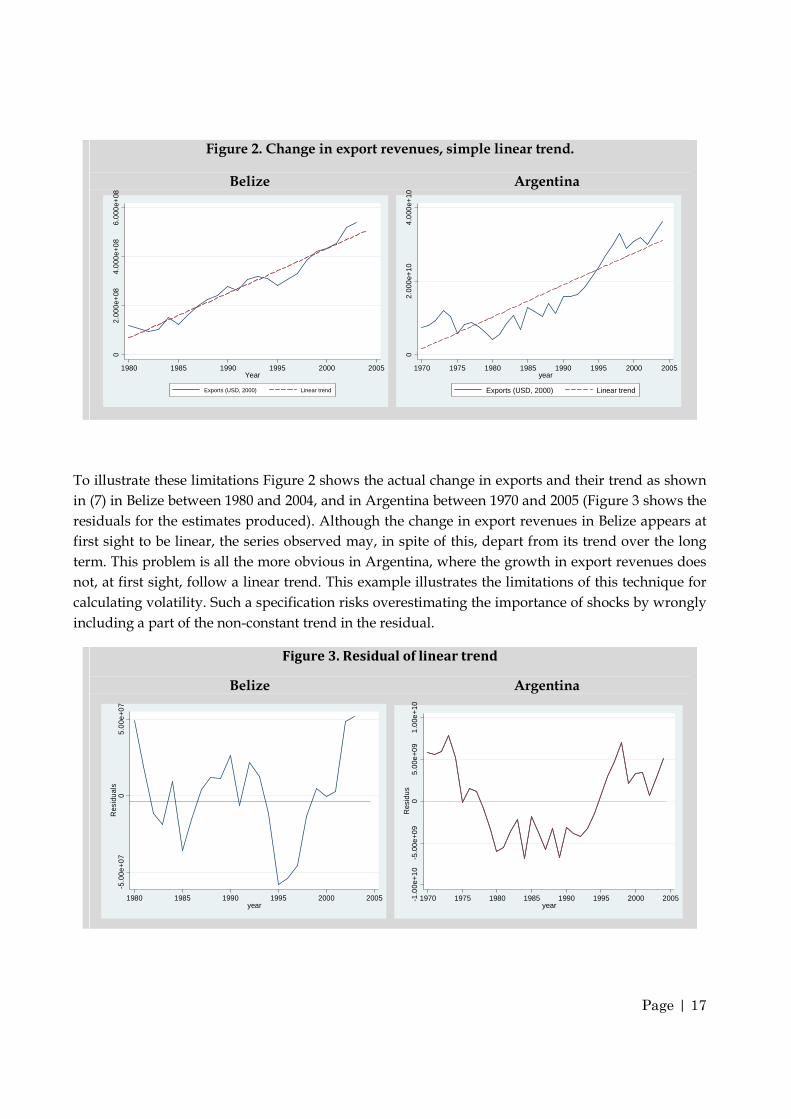
Figure 2. Change in export revenues, simple linear trend.

Belize Argentina

To illustrate these limitations Figure 2 shows the actual change in exports and their trend as shown

in (7) in Belize between 1980 and 2004, and in Argentina between 1970 and 2005 (Figure 3 shows the

residuals for the estimates produced). Although the change in export revenues in Belize appears at

first sight to be linear, the series observed may, in spite of this, depart from its trend over the long

term. This problem is all the more obvious in Argentina, where the growth in export revenues does

not, at first sight, follow a linear trend. This example illustrates the limitations of this technique for

calculating volatility. Such a specification risks overestimating the importance of shocks by wrongly

including a part of the non-constant trend in the residual.

Figure 3. Residual of linear trend

Belize Argentina

02

.000

e+08

4.0

00e+

086.

000

e+08

1980 1985 1990 1995 2000 2005Year

Exports (USD, 2000) Linear trend

02.

000

e+10

4.0

00e+

10

1970 1975 1980 1985 1990 1995 2000 2005year

Exports (USD, 2000) Linear trend

-5.0

0e+0

70

5.00

e+07

Res

idua

ls

1980 1985 1990 1995 2000 2005year

-1.0

0e+

10

-5.0

0e+0

90

5.00

e+0

91

.00e

+10

Res

idu

s

1970 1975 1980 1985 1990 1995 2000 2005year

Page | 18

Estimate based on a mixed trend

Up to this point, we have assumed that deviations from the deterministic trend are only transitory.

Equation (2), however, suggests that it is possible that residual variations (εT) are not transitory, and

have a permanent effect on the trend followed by a series. It thus becomes possible to estimate the

reference value on the basis of a stochastic trend (a random process below), represented by the

following first-order autoregressive AR(1) process,

( )21 0,N~ σεε tttt avecyy += − (6)

which we can re-write as follows:

In this case, the change in y, is determined by a successive history of random shocks, with the result

that a shock occurring in the past, even the distant past, has the same effect on the series as a shock

in the present (long-memory process). The series is then considered to be difference-stationary or that

its trend follows a random path. The series contains a unit root. After differencing, the series can be

rewritten as follows:

( )20,N~ σεε ttt avecy =∆

This hypothesis is nevertheless quite strong in the context of examining macroeconomic variables

dominated by low frequencies (Nelson and Kang, 1981). The analysis of the export series and their

spectrum in section 2.1 (see Figure 1) would justify specifying a mixed trend, suggesting the

existence of fluctuations around a trend which is both deterministic and stochastic. Namely the

process AR(1), which also includes a deterministic trend:

ttt yty εδβα +++= −1 (7)

Our aim is to discover whether the trend as specified in equation (7) makes it possible to stationarise

the export series for our sample of countries correctly. To do so, we calculate the p-value of the unit

root test using Maddala-Wu panel data (based on the Phillips Perron test), carried out in 134

countries, and Fisher statistics on the joint nullity hypothesis for coefficients associated with drift,

trend and lag (table 1).

y t = y0 + εt

1

t

∑

Page | 19

Table 1: Specification and unit root test on panel data

H0: the series is non-stationary Prob>Chi2 F-test

1.000 47.47

0.000 36.61

Countries (Observations): 134(3693).

The results of the tests carried out thus do not justify the rejection of a null hypothesis for unit root

and tend to justify the use of a mixed trend with drift (cf. equation (9)). The non-stationarity

hypothesis is thus rejected once the series is differenced for a second time, and the F-test statistics

lead us to reject the joint nullity hypothesis for the specification coefficients (9). Figure 4 illustrates

the trends obtained for the case of Belize and Argentina.

Figure 4. Change in export revenues, mixed trend.

Belize Argentina

Figure 5 shows the correlogram for the residuals of equation (7) estimated for Belize and Argentina

respectively. An examination of the correlogram shows white noise, because the correlations

associated with lags are not significantly different from zero15. With regard to these two example

countries and those shown in Appendix A.2, using a mixed trend therefore proves to be more

appropriate to stationarise export revenues.

However, an examination of Figure 4 and Appendix A.2 suggests that this method of estimating

creates a trend whose profile appears to be a slightly smoothed and offset version of the change seen

in the exports. This trend therefore seems to reproduce in t the change in exports observed in t-1,

which therefore contributes to an artificial creation of volatility. This phenomenon is all the more

marked in the cases of Argentina (Figure 4), Venezuela, Burundi and Kenya (Appendix A.2).

15The Portmanteau statistics, which are not presented in this article, do not make it possible to reject a null hypothesis for a white-noise process. They can be supplied to the reader on request.

∆yit = α i + βit + φ1yit−1 + εit

∆∆y it = α i + β it + φ2∆y it−1 + εit

02

.000

e+08

4.0

00e+

086.

000

e+08

1980 1985 1990 1995 2000 2005year

Exports (USD, 2000) Mixed trend

02

.000

e+10

4.00

0e+

10

1970 1975 1980 1985 1990 1995 2000 2005year

Exports (USD, 2000) Mixed trend

Page | 20

Figure 5. Correlogram of residuals, mixed trend

Belize Argentina

Estimate based on a rolling mixed trend

The main problem with a mixed trend as calculated in the previous sub-section is that it is based on

a strong hypothesis of constancy over time of the coefficients associated with the trend of the series.

Effectively, this so-called “global” trend is predicted each year for each country based on coefficients

estimated for the whole period of data availability. It also excludes the possibility of a change of

regime in the deterministic and stochastic change of the series concerned. Maddala and Kim (1996)

emphasise that important changes in the deterministic component of the trend taken by a series can

lead, wrongly, to a failure to reject the unit root hypothesis. It is therefore possible that the mixed

trend we have estimated attributes to random trend variations a change in the deterministic change

of the series, which may then lead to an overestimate of the magnitude of fluctuations. Although

tests do exist (e.g. CUSUM, Max Chow) to identify breaks in a trend during unit root tests (Maddala

and Kim, 1996), an alternative and practical solution is to produce a “rolling” estimate of the mixed

trend over a shorter period (Guillaumont, 2007), allowing the coefficients estimated to change from

year to year and thus reflecting recent changes in the series trend. This “rolling mixed trend” is

calculated for each country and each year based on estimating equation (9) over the period [t; t-k],

rather than over the whole of the period:

1ˆˆˆˆ −++= t

TTTTt yty δβα

(8)

and tTtt yy ε+= ˆ

where T is the estimation period for the trend corresponding to (t; t – k).

The results obtained when k = 12 are shown for Argentina in Figure 6 and compared with those

obtained based on the previous “global” mixed trend. Appendix A.2 shows the predictions and

-0.4

0-0

.20

0.00

0.20

0.40

Aut

ocor

rela

tions

1 2 3 4 5 6Lags

Bartlett's formula for MA(q) 95% confidence bands

-0.4

0-0

.20

0.00

0.20

0.40

Aut

ocor

rela

tions

1 2 3 4 5 6Lags

Bartlett's formula for MA(q) 95% confidence bands

Page | 21

correlograms for residuals obtained using global and rolling mixed trends for other country

examples. We can see that the trend thus obtained is smoother than with the previous model and

that it does not have a “sawtooth” profile resulting from constant parameters over time. Similarly,

an examination of the correlogram in Figure 6 and Figure 7, and the correlograms in the appendix

(Appendix A.2), suggests that the residuals resulting from this approach are stationary for the

country examples chosen.

Figure 6. Rolling mixed trend, comparative change and correlogram of residuals, Argentina.

Nonetheless, this technique presents a number of disadvantages. On the one hand, it reduces the

time coverage of volatility indicators, since the first trend value is only available from t = 1+k. On

the other hand, a bias may appear as the result of a limited trend estimation period.

Estimates based on a rolling mixed trend are not necessarily an ideal solution where there is a break

in the trend of the series. Changes prior to the break may continue to exhibit inertia when the rolling

trend is estimated, once the break has occurred. Moreover, by proposing an estimate of the trend

over a shorter period than the global mixed trend, this technique may include some long-periodicity

fluctuations in the residual as a result of being more sensitive to medium-periodicity fluctuations.

This phenomenon is illustrated in particular by the respective behaviour of two mixed trends

applied to Burundi between 1985 and 1995 in Figure 7. The rolling mixed trend tends to

underestimate the trend for exports to fall relative to the “global” trend over the same period.

The choice of period for calculating the trend is therefore important. In this case we have chosen an

estimation period for the rolling trend of 12 years, in order to highlight the advantages and

disadvantages of this technique compared with the global mixed trend. It could be considered that a

rolling trend calculated over a period of between 10 and 20 years represents a reasonable basis with

regard to the spectrum densities presented previously in Figure 1, since medium-term fluctuations

seem to contribute strongly to the total variability of the series. This choice should be justified based

on a prior examination of series behaviour (unit root tests, graphical examination of series and

examination of their spectrum density) and supported by a study of the literature on the topic.

02.

000

e+10

4.0

00e+

10

1970 1980 1990 2000year

Exports (USD, 2000) Global mixed trend

Rolling mixed trend

-0.5

00.

000.

50A

utoc

orre

latio

ns

1 2 3 4 5 6Lags

Bartlett's formula for MA(q) 95% confidence bands

Page | 22

2.3. Filtering approach

Some research on economic volatility uses a statistical filtering approach to isolate the cyclical and

trend components of changes in the series (Becker and Mauro, 2006; Chauvet and Guillaumont,

2007). The standard deviation of the cyclical component then becomes an example of a volatility

indicator. The most popular filter remains the Hodrick-Prescott filter (1997). This can stationarise

potentially integrated series up to order four (King and Rebelo, 1993). The band-pass (BP) filter put

forward by Baxter and King (1999) is also used in the literature on economic fluctuations

(Hnatkovska and Loayza, 2005). Although the BP filter maintains the properties of the series more

accurately, this advantage comes at the price of a loss of observations at the end of the sample16

(Baxter and King, 1999). Moreover, when applied to our export data, both techniques give extremely

similar results17. In this article we therefore only present the results obtained with the Hodrick-

Prescott (HP) filter.

The advantage of the filtering method compared with those described above is that it does not

impose a priori any particular (and sometimes arbitrary) form (mixed trend, deterministic, random,

etc.) on the behaviour of the series. Moreover, a statistical filtering method enables changes to the

trend over time, which is a definite advantage over the time series-based approach we have

16The BP filter is a bilateral filter, which requires a minimum number of observations before and after each filtered observation point in order to increase the precision of the filtering. Baxter and King recommend ignoring the first 12 and last 12 quarters when filtering quarterly series. For annual series, they recommend ignoring the first three and last three years of the sample.

17Available to the reader on request.

Figure 7. Global and rolling mixed trends, comparative change and correlogram of residuals,

Burundi.

5000

0000

1.00

0e+

081.

500e

+08

2.00

0e+

08

1970 1980 1990 2000year

Exports (USD, 2000) Global mixed trend

Rolling mixed trend

-0.5

00.

000.

50A

utoc

orre

latio

ns

1 2 3 4 5 6Lags

Bartlett's formula for MA(q) 95% confidence bands

Global mixed trend

-0.5

00.

000.

50A

utoc

orre

latio

ns

1 2 3 4 5 6Retards

Bartlett's formula for MA(q) 95% confidence bands

Rolling mixed trend

Page | 23

presented. Hodrick and Prescott break down the change in a series into a non-stationary trend

component (yPt), and a stationary cyclical component (yCt):

yt = yPt + yCt , T = 1, 2, 3,…, t. (9)

The HP filter consists of isolating the cyclical component by optimising the following programme in

relation to Yp:

(10)

It is similar to a symmetrical infinite moving average filter. The parameter λ is called a “smoothing

parameter”. The first term of the equation (10) minimises variance in the cyclical component (YCt)

whilst the second term smoothes the change in the trend component. When λ tends towards infinity,

the variance in the growth of the trend component tends towards 0, which implies that the trend

component – or filtered series – is close to a simple linear temporal trend. Conversely, when λ tends

toward 0, the filtered series is close to the original series. Isolated cyclical fluctuations will thus

exhibit a higher (short) frequency (periodicity) the lower the value of the smoothing parameter.

The choice of the value of λ remains arbitrary and there is as yet no unanimity in the literature.

Whilst Hodrick and Prescott advocate a parameter λ equal to 100 for annual data, some studies

suggest a higher value, of between 100 and 400 (Baxter and King, 1999), whilst others prefer

significantly lower values, of between 6 and 10 (Maravall and Del Rio, 2001). Given that the aim of

this article is not to debate the appropriate value for the smoothing parameter, we will compare the

results obtained when it is equal to 100 and 6.5. We will thus obtain deviations compared with a

long-term trend (λ=100) and a medium-term trend (λ=6.5).

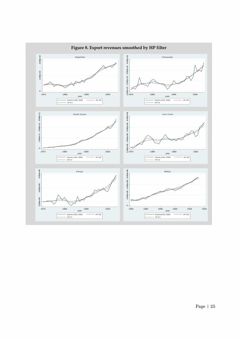
An examination of Figure 8 suggests that use of the HP filter can apply to a large number of

countries with varied profiles for changes in exports. As predicted, values filtered with a smoothing

parameter of 6.5 are more sensitive to fluctuations in the medium term than those filtered with a

parameter of 100. Appendix A.3 shows the correlograms between the cycles of the countries shown

in Figure 8. Both these figures thus suggest that the cycles extracted are stationary and not

significantly autocorrelated. The p-values of the Phillips-Perron test below the correlograms in

Appendix A.3 show that we can reject the null hypothesis for first-order integration of the cycle with

a confidence interval of 99%, which indicates that the series seems to be correctly stationarised for

these countries with this technique.

The approach nonetheless presents a number of disadvantages. Whilst this method does not impose

a particular functional form on the change in the trend, it does impose, in an ad hoc manner,

weightings identical to the values before and after the filtered value. It thus suggests the hypothesis

that the cyclical component and trend component of economic series are independent. In light of the

significant amount of research on the effects of macroeconomic volatility on long-term growth,

however, this hypothesis seems restrictive. Moreover, a further defect of the HP filter is that it

becomes unilateral at the end of the sample, thus giving less good results at the start and end of the

minYt

p{ }t=1

TYt −Yt

p( )2+ λ ∆2Yt

p( )2

t= 2

T −1

∑t=1

T

∑

Page | 24

data availability period (Van Norden, 2004). Finally and above all, as regards the choice of a

smoothing parameter, a low value provokes compression effects: part of the short-periodicity cyclical

variation can be attributed to the trend. The estimated trend then appears to be highly volatile and

the cyclical component – and therefore volatility – may be underestimated in this case. Conversely,

the choice of a high smoothing parameter provokes leakage effects: some of the long-periodicity

variations can be attributed to the cyclical component. The trend thus appears less volatile and the

cyclical component tends to be overestimated. As regards macroeconomic volatility in developing

countries, an examination of the spectra of the export series in Figure 1 suggests the choice of a low

smoothing parameter, given the significance of medium-term fluctuations. Figure 8 shows a

graphical representation of the consequences of choosing a high or low smoothing parameter.

As we have seen in this section, the method of calculation used for the reference value is central to

calculating volatility. If we wish to reflect the effects of transitory variations – for example due to

economic cycles, certain commercial shocks or climatic events – it is essential to use an adequate

series stationarisation method. In this regard we have set out the two main approaches adopted in

the literature on macroeconomic volatility: the parametric approach and the filtering approach.

Although both these approaches provide acceptable results in relation to stationarisation, the global

mixed trend seems to create volatility artificially: this is less true of the rolling mixed trend and the

filtering method.

Page | 25

Figure 8. Export revenues smoothed by HP filter

02.0

00e+

104.

000

e+10

1970 1980 1990 2000year

Exports (USD, 2000) HP 100

HP 6.5

Argentina

1.0

00e+

102.0

00e+

103.

000

e+10

4.000

e+10

1970 1980 1990 2000year

Exports (USD, 2000) HP 100

HP 6.5

Venezuela

01.0

00e+

112.

000

e+11

3.000

e+11

1970 1980 1990 2000year

Exports (USD, 2000) HP 100

HP 6.5

South Korea

2.0

00e+

094.0

00e+

096.

000

e+09

8.0

00e+

09

1970 1980 1990 2000year

Exports (USD, 2000) HP 100

HP 6.5

Ivory Coast

2.000

e+09

3.0

00e+

094.0

00e+

09

1970 1980 1990 2000year

Exports (USD, 2000) HP 100

HP 6.5

Kenya

02.0

00e+

084.0

00e+

086.0

00e+

08

1980 1985 1990 1995 2000 2005year

Exports(USD, 2000) HP 100

HP 6.5

Belize

Page | 26

3. Calculating deviation from the trend

Unlike shock variables, which reflect instantaneous fluctuations, measuring volatility involves

calculating a deviation which reflects an accumulation of fluctuations. The deviations presented in

this section consist of summing the deviations around a trend over a given period, so as to highlight

a particular aspect of the distribution of a variable (stationary or stationarised): its variance,

asymmetry or degree of kurtosis (or flattening) of the distribution.

Limiting the analysis of volatility only to traditional indicators based on the variance of a variable,

such as standard deviation or the coefficient of variation18, can mask other important aspects of

volatility, such as the asymmetry of deviations and the occurrence of extreme deviations. In fact,

measures such as the standard deviation of deviations, which measure the average magnitude of a

distribution, do not take account of the asymmetry of the reactions of economic agents to positive or

negative shocks. Similarly, they are not able to identify whether the distribution around the trend is

characterised by frequent shocks on a limited scale, or dominated by infrequent shocks on a large

scale. These characteristics of a distribution are important, however, if, for example, the aim is to

study how volatility affects the behaviour of economic agents. We present below the possible

options for quantifying these phenomena, based on the various moments of distributions around

the reference values presented in the previous section.

3.1. Calculation period for volatility

If an indicator of volatility is intended to reflect past experience of shocks, the choice of period over

which the deviation is calculated is a first step towards calculating said deviation. If, for example,

the aim is to examine the short-term effects of volatility, it is common to calculate an indicator

reflecting fluctuations over the last five or ten years. If the aim is to study the medium/long-term

effects of volatility, a calculation period of over ten years may be needed. Moreover, where the

change in a series presents distinct episodes of volatility over time, it may be relevant to align the

period over which deviations are summed to the approximate period of the episodes of volatility

(Wolf, 2005). In fact it is possible to sum over a short period, deviations around a trend which has

itself been estimated over a longer period (see section 2.2). In this case, it will be a matter of studying

the short-term effects of fluctuations around a shorter- or longer-term trend.

In the remainder of the document, we compare the results from different types of volatility

indicators used to analyse the three dimensions (or moments) of the distribution of a variable: the

scale of values of a variable, their asymmetry and the occurrence of extreme deviations.

18Their respective formulae are set out at the end of this section.

Page | 27

3.2. The magnitude of volatility

Numerous research articles cited in the list of references examine the consequences and

determinants of the magnitude of volatility. Several methods are available to quantify this aspect of

volatility. The most common method consists of calculating the standard deviation of a variable

based on its reference value:

∑

−×=

t t

tt

y

yy

TINS

2

1 ˆ

ˆ1100

with T=1, …, t.

We compare the deviations with the reference value in order to ensure comparability between the

indicators of volatility of a variable whose order of magnitude differs from one country to another.

It is also possible to calculate the average absolute deviation of deviations from the trend:

∑−

×=t t

tt

y

yy

TINS

ˆ

ˆ11002

with T=1, …, t.

Where ty is the observed value of the series, and ty is the reference value. The question of the

respective advantages of standard deviation and absolute average to measure the ‘average

deviation’ of a distribution is an old debate (Gorard, 2005). The preference for standard deviation is

historic and is related in part to the fact that numerous statistical tests and numerous indicators are

based on it. The preference arose because i) it was shown that in the case of a normal/Gaussian

distribution, standard deviation provides a more efficient estimate of ‘average deviation’ than

average absolute deviation; and ii) it is easier to manipulate in algebraic terms. In the context of an

economic analysis of the effects of the magnitude of volatility, the use of standard deviation is

justified in the case where the effects of volatility increase exponentially with the size of fluctuations.

It has been shown, however, that average absolute deviation is a more efficient measure where there

are measuring errors, or when the distribution is not normal. We illustrate the differences between

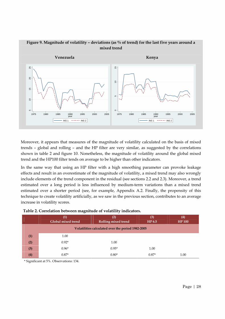
these two measures of the magnitude of volatility based on the results obtained for Venezuela and

Kenya shown in Figure 9. Both of these measures are calculated on a rolling annual basis over a

calculation period of five years (t; t-5). Figure 9 suggests that the peaks of volatility corresponding to

the end of the 1970s, 1980s and the early 1990s and 2000s are more heavily weighted when we use

the mean square deviation (INS1).We subsequently prioritise use of the standard deviation (INS1) as

a measure of the average magnitude of deviations, given that this method of calculation makes it

possible to distinguish more easily between different episodes of volatility, because of its frequent

use in the literature and because the other measures of volatility presented in the paper are based on

this statistic. We then compare the standard deviations obtained from the reference values presented

in the previous section. This time, deviations are calculated over the period 1982-2005. The results

are shown in tables 2 and 3, and in figure 10.

Page | 28

Figure 9. Magnitude of volatility – deviations (as % of trend) for the last five years around a

mixed trend

Venezuela Kenya

Moreover, it appears that measures of the magnitude of volatility calculated on the basis of mixed

trends – global and rolling – and the HP filter are very similar, as suggested by the correlations

shown in table 2 and figure 10. Nonetheless, the magnitude of volatility around the global mixed

trend and the HP100 filter tends on average to be higher than other indicators.

In the same way that using an HP filter with a high smoothing parameter can provoke leakage

effects and result in an overestimate of the magnitude of volatility, a mixed trend may also wrongly

include elements of the trend component in the residual (see sections 2.2 and 2.3). Moreover, a trend

estimated over a long period is less influenced by medium-term variations than a mixed trend

estimated over a shorter period (see, for example, Appendix A.2. Finally, the propensity of this

technique to create volatility artificially, as we saw in the previous section, contributes to an average

increase in volatility scores.

Table 2. Correlation between magnitude of volatility indicators.

(1)

Global mixed trend

(2)

Rolling mixed trend

(3)

HP 6.5

(4)

HP 100

Volatilities calculated over the period 1982-2005

(1) 1.00

(2) 0.92* 1.00

(3) 0.96* 0.95* 1.00

(4) 0.87* 0.80* 0.87* 1.00

* Significant at 5%. Observations: 134.

510

1520

25

1975 1980 1985 1990 1995 2000 2005year

INS 1 INS 2

05

1015

1975 1980 1985 1990 1995 2000 2005year

INS 1 INS 2

Page | 29

Table 3. Descriptive statistics of magnitude of volatility indicators (%).

Volatility Mixed trend Volatility Rolling Mixed

trend

Volatility HP 6.5 Volatility HP 100

Mean 13.6 11.5 9.2 13.3

Standard

deviation 8.7 7.8 6.1 7.8

Observations: 134.

The values smoothed by the HP filter are calculated on the basis of a symmetric moving-average

process and used to take account of any breaks in the trend. It has been noted that the trend in the

numerous developing countries which make up our sample is more volatile (Rand and Tarp, 2002).

This is why the use of the HP(100) filter is relevant if the aim is to reflect the trend in exports in

industrialised economies, over a longer period and on a larger scale. As with the global mixed trend,

the HP100 filter is therefore less sensitive than other trends to variations over a medium period. This

explains why volatility calculated on the basis of the HP100 filter correlates less closely – though still

at a high level of around 80% – and shows a higher mean than other methods.

Figure 10. Graphical illustration of correlations between magnitude of volatility indicators.

ALB

DZAAGOATGARG

AUSAUTBHRBGD

BRBBELBLZBENBTNBOLBWA

BRABGRBFA

BDI

CMR

CANCAF

TCD

CHLCHNCOL

COMCOG

ZAR

CRICIVCYPDNKDMA

DOM

ECUEGYSLVETHFJIFINFRA

GABGMB

DEU

GHA

GRCGTM

GNB

GUY

HTI

HNDHKGHUNISLINDIDN

IRN

IRLISRITAJAMJPNJORKEN

KIR

KOR

KWT

LAO LSOLUXMAC

MDGMWI

MYSMLIMLTMRTMUSMEXMARMOZNAMNPLNLDNZL

NICNER

NGA

NOR

OMNPAKPAN

PNGPRYPERPHLPRTPRI

RWASTPSAU

SENSYC

SLE

SLBSOM

ZAFESPLKAKNALCAVCT

SURSWZ

SWECHESYR

THATGOTON

TTOTUNTUR

UGA

ARE

GBRUSAURY

VUTVENZMBZWE

020

4060

Glo

bal m

ixed

tre

nd

0 20 40 60 80Rolling mixed trend

ALB

DZAAGOATGARGAUS

AUTBHRBGDBRBBELBLZBENBTNBOLBWA

BRA

BGRBFABDI

CMRCAN

CAF

TCD

CHLCHNCOL

COMCOG

ZAR

CRICIVCYPDNK

DMA

DOM

ECUEGYSLVETHFJIFINFRA

GABGMBDEU

GHA

GRCGTM

GNB

GUY

HTI

HNDHKGHUNISLINDIDN

IRN

IRLISRITAJAMJPNJORKEN

KIR

KOR

KWT

LAO

LSOLUXMAC

MDGMWIMYSMLIMLTMRTMUSMEXMAR

MOZNAMNPL

NLDNZL

NICNER

NGA

NOROMN

PAKPANPNGPRYPER

PHLPRTPRI

RWASTP

SAU

SENSYC

SLE

SLB

SOM

ZAFESPLKA

KNALCAVCT

SUR

SWZSWECHESYRTHA

TGOTONTTO

TUNTUR

UGA

AREGBRUSA

URYVUT

VENZMBZWE

010

2030

40

50H

P10

0

0 10 20 30 40 50HP65

ALB

DZAAGOATGARG

AUSAUTBHRBGD

BRBBELBLZBENBTNBOLBWA

BRABGRBFA

BDI

CMR

CANCAF

TCD

CHLCHNCOL

COMCOG

ZAR

CRICIVCYPDNKDMA

DOM

ECUEGYSLVETHFJIFINFRA

GABGMB

DEU

GHA

GRCGTM

GNB

GUY

HTI

HNDHKGHUNISLINDIDN

IRN

IRLISRITAJAMJPNJORKEN

KIR

KOR

KWT

LAOLSOLUXMAC

MDGMWI

MYSMLIMLTMRTMUSMEXMARMOZNAMNPLNLDNZL

NICNER

NGA

NOR

OMNPAKPAN

PNGPRYPERPHLPRTPRI

RWASTPSAU

SENSYC

SLE

SLBSOM

ZAFESPLKAKNALCAVCT

SURSWZ

SWECHESYR

THATGOTON

TTOTUNTUR

UGA

AREGBRUSA

URYVUTVENZMBZWE

020

40

60G

loba

l mix

ed

tren

d

0 10 20 30 40 50HP65

ALB

DZAAGOATGARG

AUS AUTBHRBGD

BRBBELBLZBENBTNBOLBWA

BRABGRBFA

BDI

CMR

CANCAF

TCD

CHLCHNCOL

COMCOG

ZAR

CRICIVCYPDNKDMA

DOM

ECUEGYSLVETHFJIFINFRA

GABGMB

DEU

GHA

GRCGTM

GNB

GUY

HTI

HNDHKGHUNISLINDIDN

IRN

IRLISRITAJAMJPNJORKEN

KIR

KOR

KWT

LAOLSOLUXMAC

MDGMWI

MYSMLIMLTMRTMUSMEXMAR MOZNAMNPLNLDNZL

NICNER

NGA

NOR

OMNPAKPAN

PNGPRYPERPHLPRTPRI

RWASTP SAU

SENSYC

SLE

SLBSOM

ZAFESPLKA KNALCAVCT

SURSWZ

SWECHESYR

THATGO

TON

TTOTUNTUR

UGA

AREGBRUSA

URYVUTVENZMBZWE

020

40

60G

loba

l mix

ed

tren

d

0 10 20 30 40 50HP100

ALBDZAAGO

ATGARG

AUSAUTBHRBGDBRBBELBLZBENBTNBOLBWABRA

BGRBFABDICMRCAN CAF

TCD

CHLCHNCOLCOM

COGZARCRICIVCYPDNK DMA

DOM

ECUEGYSLVETHFJIFINFRAGAB

GMBDEU

GHA

GRCGTM

GNBGUY

HTI

HNDHKGHUNISLINDIDN

IRN

IRLISRITAJAMJPNJORKEN

KIR

KOR

KWT

LAOLSO

LUXMAC MDGMWIMYSMLIMLTMRTMUSMEXMARMOZNAMNPLNLDNZLNICNER

NGA

NOROMN

PAKPANPNGPRYPER

PHLPRTPRI

RWASTPSAU

SENSYC

SLESLB

SOM

ZAFESPLKAKNALCAVCTSUR

SWZSWECHESYRTHA

TGOTONTTOTUNTUR

UGA

AREGBRUSA URY VUT

VENZMBZWE

020

40

6080

Rol

ling

mix

ed tre

nd

0 10 20 30 40 50HP65

ALBDZAAGO

ATGARG

AUS AUTBHRBGDBRBBELBLZBENBTNBOLBWABRA

BGRBFABDICMRCAN CAF

TCD

CHLCHNCOLCOM

COGZARCRICIVCYPDNKDMA

DOM

ECUEGYSLVETHFJIFINFRAGAB

GMBDEU

GHA

GRCGTM

GNBGUY

HTI

HNDHKGHUNISLINDIDN

IRN

IRLISRITAJAMJPNJORKEN

KIR

KOR

KWT

LAOLSO

LUXMAC MDGMWIMYSMLIMLTMRTMUSMEXMAR MOZNAMNPLNLDNZLNICNER

NGA

NOROMN

PAKPANPNGPRYPER

PHLPRTPRI

RWASTP SAU

SENSYC

SLESLB

SOM

ZAFESPLKA KNALCAVCTSUR

SWZSWECHESYRTHA

TGOTONTTOTUNTUR

UGA

AREGBRUSA URY VUT

VENZMBZWE

020

40

6080

Rol

ling

mix

ed tre

nd

0 10 20 30 40 50HP100

Page | 30

3.3. The asymmetry of volatility

Measures of magnitude do not provide a means of identifying the effects of the asymmetry of

shocks (Wolf, 2005). A study of the effects of the asymmetry of fluctuations is justified, however, in

light of the distinction in agents’ responses to negative or positive shocks (Dercon, 2002; Elbers et al,

2007). The coefficient of asymmetry or skewness, describes the macroeconomic volatility profile

facing a country, since it indicates the propensity of countries to suffer negative or positive shocks.

This value is calculated as follows:

tTavec

y

yy

T

y

yy

TSkewness

t t

tt

t t

tt

,...,1

ˆ

ˆ1

ˆ

ˆ1

1002/32

3

=

−

−

×=

∑

∑

A negative skewness indicates that the distribution is weighted towards the left of the reference

value, whilst a positive coefficient indicates a distribution weighted towards the right (see figure

11). A symmetrical distribution will have a coefficient whose value is close to zero. A distribution

with a positive (negative) skewness therefore indicates an experience of volatility dominated by

positive (negative) shocks. Moreover, asymmetry increases as shocks (whether positive or negative)

become greater. In other words, skewness also indicates the propensity of a variable to undergo

crises (when negative) or booms (when positive) (Rancière et al, 2008).Although the measures of the

magnitude of deviations around a trend presented previously are strongly correlated (see table 2

and figure 10), the asymmetry of distributions of deviations around them can present a significantly

different profile depending on the reference value chosen (see Table 4). Thus, for a given magnitude

of volatility, the experience of shocks of two different countries can present a contrasting asymmetry

(see figure 11).

Figure 11 Graphical illustration of a positive and negative

asymmetric distribution of identical magnitude19.

19Source: Wikipedia.fr.

Page | 31

Table 4 shows that the correlations between skewness based on different values are weak, which suggests that each of the reference values expresses the asymmetry of shocks differently. The similarity in the profile of distributions of deviations around the filtered values is confirmed by a relatively strong correlation between their skewness (65%), whilst the skewness obtained from the global mixed trend is weakly correlated to the others. The asymmetry of the distribution of results around the mixed trend shows correlations with other, weaker indicators (14% with the skewness-HP(6.5), and 2% with the skewness-HP(100)).

Table 4. Correlations of coefficients of asymmetry calculated over the period 1982-2005.

(1) skewness (Global mixed

trend)

(2) skewness (Rolling mixed

trend)

(3) skewness (HP(6.5))

(4) skewness (HP(100))

Skewness calculated over the period 1982-2005

(1) 1

(2) 0.23* 1

(3) 0.08* 0.14* 1

(4) 0.29* 0.02 0.65* 1

* Significant at 10%. Sample = 134 countries.

Figure 12 compares indicators of the magnitude of volatility with indicators of the asymmetry of volatility for each reference value. The straight-line correlations obtained for each reference value suggest a fairly weak positive correlation, particularly if certain outliers are excluded. This graph underlines the fact that for episodes of volatility on a similar magnitude, the asymmetry of shocks may be opposite, suggesting an entirely distinct experience of shock.

The asymmetry of distributions around the reference value is therefore a separate aspect of volatility, which cannot only be assessed by the indicators of magnitude presented in section 3.2.

Page | 32

Figure 12. Correlation between magnitude and asymmetry of volatility indicators, by reference value.

AGO

ALB

AREARG

ATG

AUS AUT

BDI

BELBEN

BFABGDBGRBHRBLZ BOL

BRABRBBTNBWACAF

CANCHECHL

CHNCIV

CMRCOG

COL

COM

CRICYPDEU

DMA

DNK

DOM

DZA

ECUEGY ESPETHFINFJI

FRA

GAB

GBR

GHA

GMB

GNB

GRCGTMGUY

HKGHND

HTI

HUNIDN IND IRL

IRN

ISLISR ITAJAMJORJPNKEN

KIR

KNAKOR

KWT

LAOLCA

LKA

LSO

LUXMAC MAR

MDG

MEX MLIMLTMOZ MRTMUSMWI

MYS NAMNER

NGA

NIC

NLDNOR

NPLNZL

OMN

PAKPANPER

PHL

PNG

PRI PRT

PRY

RWASAU

SEN

SLB

SLE

SLV

SOM

STPSUR

SWE

SWZ

SYCSYR

TCD

TGOTHA

TON

TTOTUN

TUR

UGA

URYUSA

VCTVEN VUT

ZAF

ZAR

ZMBZWE

020

4060

-100 0 100 200 300Asymmetry

Global mixed trendCorrelation = 23%

Mag

nitu

de

AGO

ALB

AREARG

ATG AUSAUTBDI

BELBENBFA BGDBGRBHRBLZ BOL

BRABRB BTNBWACAFCAN CHECHLCHN

CIVCMRCOGCOL

COM

CRICYP DEUDMADNK

DOMDZA

ECUEGYESP

ETHFINFJI FRA

GAB

GBR

GHA

GMB

GNB

GRCGTMGUY

HKGHND

HTI

HUNIDN INDIRL

IRN

ISLISR ITA JAMJOR JPN KEN

KIR

KNA KOR

KWT

LAO LCA LKALSO

LUXMACMARMDGMEX MLIMLTMOZMRTMUSMWI

MYS NAMNER

NGA

NIC

NLDNORNPL

NZLOMN

PAKPANPER

PHLPNG

PRIPRTPRY

RWASAU

SENSLB

SLE

SLV

SOM

STPSUR

SWESWZ

SYCSYR

TCD

TGO

THA

TONTTO

TUNTUR

UGA

URYUSA

VCT VENVUTZAF

ZARZMB

ZWE0

2040

6080

-200 -100 0 100 200 300Asymmetry

Rolling mixed trendCorrelation = 36%

Mag

nitu

de

AGO

ALB

AREARG

ATGAUSAUT

BDI

BEL

BENBFA

BGD BGRBHRBLZ BOLBRABRB

BTNBWA CAF

CANCHECHL CHN

CIV CMRCOG

COL

COM

CRICYPDEU

DMADNK

DOM

DZAECUEGY

ESPETH

FINFJIFRA

GAB

GBR

GHA

GMB

GNB

GRC GTMGUY

HKGHND

HTI

HUNIDN INDIRL

IRN

ISL ISRITAJAM JORJPN KEN

KIR

KNA KOR

KWT

LAOLCA LKA

LSO

LUX MAC MAR

MDGMEXMLIMLT

MOZMRTMUS

MWI

MYSNAMNER

NGA

NIC

NLD NORNPL

NZL

OMN

PAKPAN

PER

PHL

PNG

PRIPRTPRY

RWASAU

SEN

SLB

SLE

SLV

SOM

STPSUR

SWESWZ

SYCSYR

TCD

TGO

THA

TONTTO

TUNTUR

UGA

URYUSA

VCTVEN VUT

ZAF

ZAR

ZMBZWE

010

2030

4050

-200 -100 0 100 200Asymmetry

HP 6.5

Correlation = 18%

Mag

nitu

de

AGO

ALB

ARE ARGATG

AUSAUT

BDI

BELBEN

BFA

BGD

BGR

BHRBLZ BOLBRA BRB

BTNBWACAF

CANCHECHL CHN

CIV CMRCOG

COL

COM

CRICYP

DEUDMA

DNK

DOM

DZAECUEGY

ESP

ETHFINFJIFRA

GAB

GBR

GHA

GMB

GNB

GRCGTM

GUYHKG HND

HTI

HUNIDNINDIRL

IRN

ISLISRITA

JAM JORJPNKEN

KIR

KNAKOR

KWT

LAO

LCALKA

LSO

LUXMACMAR

MDG MEXMLIMLTMOZ

MRTMUSMWI

MYSNAM

NER

NGA

NIC

NLD NORNPL

NZL

OMN

PAKPAN

PERPHL

PNG

PRIPRT

PRYRWASAU

SEN

SLB

SLE

SLV

SOM

STP

SUR

SWESWZ

SYCSYR

TCD

TGO

THATON

TTOTUN TUR

UGA

URY

USA

VCTVENVUT

ZAF

ZAR

ZMBZWE

010

2030

4050

-200 -100 0 100 200 300Asymmetry

HP 100Correlation = 38%

Mag

nitu

de

Page | 33

3.4. Frequency of extreme deviations

A final dimension of the volatility of a macroeconomic variable is the occurrence of extreme

deviations within a given distribution. This is measured by the fourth moment of the distribution of

observations around their reference value, namely kurtosis. This value is calculated as a percentage

of the reference value, as follows:

tTavec

y

yy

T

y

yy

TKurtosis

t t

tt

t t

tt

,...,1

ˆ

ˆ1

ˆ

ˆ1

10022

4

=

−

−

×=

∑

∑

In the case of a normal distribution,

kurtosis is equal to 3 (or 300% when

expressed as a percentage of the

trend). The kurtosis is a measure of

both the peakedness and tails’

fatness of a random variable’s

probability distribution relative to

those of a normal distribution. It

indicates the extent to which the

number of observations close to the

mean is high compared with

observations away from the mean.

In other words, a high value

indicates that the distribution tends

to be pointed around the mean with

thick tails. A low coefficient indicates that the distribution tends to be concentrated around the mean

with thin tails. Figure 13 illustrates three types of flattening of distributions – leptokurtic (kurtosis >

3), normal (kurtosis = 3), and platikurtic (kurtosis < 3). This thus gives an indication of the

propensity of a variable to take high values. The risk of kurtosis is seen as a major risk in finance

and on this basis is used as a measure of volatility in its own right. In the case of export volatility, it

makes it possible to have an idea of the propensity of certain countries to experience significant

variations in foreign trade in terms of volume or prices. As underlined by Rancière et al (2008), a

high value of kurtosis should be interpreted with caution since it may both “be generated either by

extreme events or by a cluster of observations around the mean that affect the peakedness of the

distribution” (p.386). They find that about one-fifth of their sample of countries exhibiting high

kurtosis was affected by observations in the neighbourhood of the distribution centre. One should

hence look carefully at country data and combine such measure of volatility with a measure of

skewness, to ensure that countries actually experienced sharp unusual fluctuations (see figure 15).

Figure 15 also illustrates that such combination can reflect country’s propensity to experience

Figure 13. Graphic representation of the degree of

flattening of a distribution

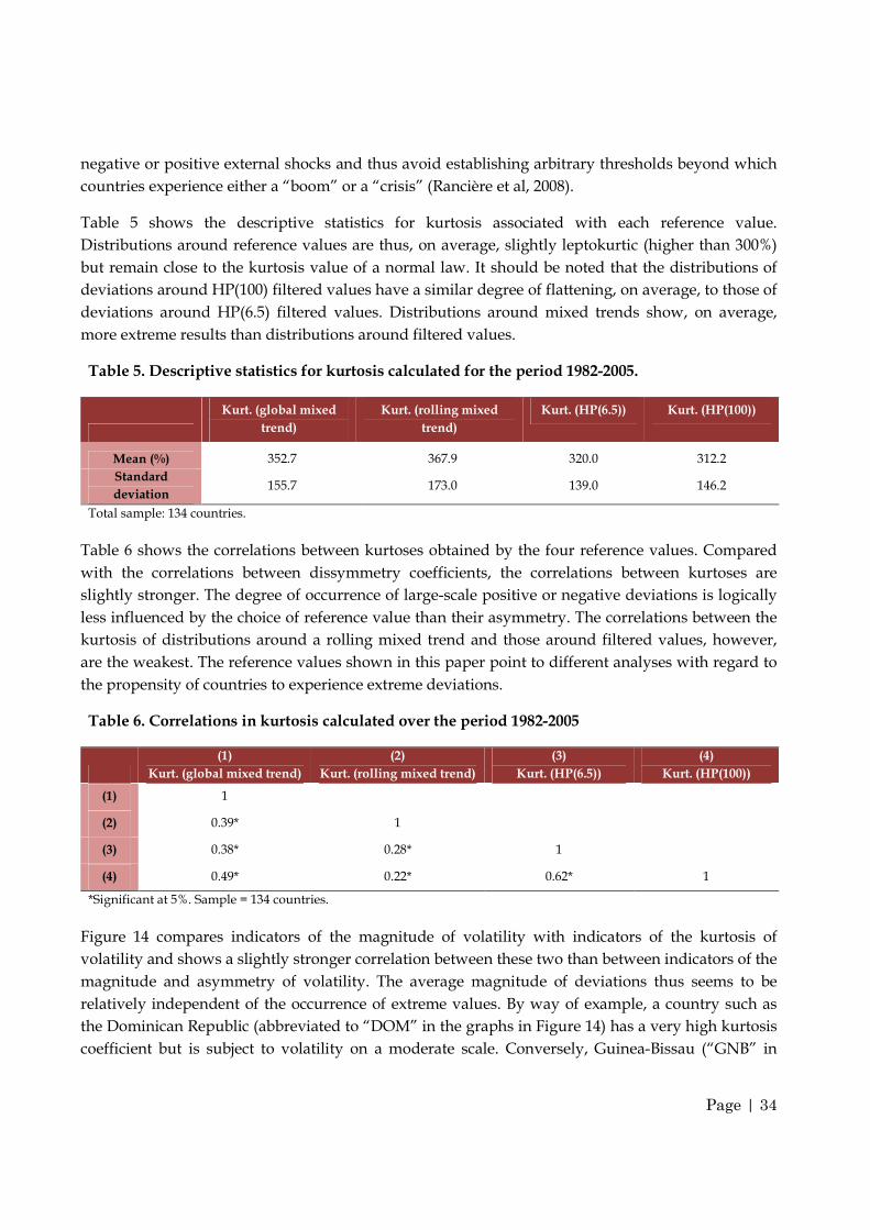
Page | 34

negative or positive external shocks and thus avoid establishing arbitrary thresholds beyond which

countries experience either a “boom” or a “crisis” (Rancière et al, 2008).

Table 5 shows the descriptive statistics for kurtosis associated with each reference value.

Distributions around reference values are thus, on average, slightly leptokurtic (higher than 300%)

but remain close to the kurtosis value of a normal law. It should be noted that the distributions of

deviations around HP(100) filtered values have a similar degree of flattening, on average, to those of

deviations around HP(6.5) filtered values. Distributions around mixed trends show, on average,

more extreme results than distributions around filtered values.

Table 5. Descriptive statistics for kurtosis calculated for the period 1982-2005.

Kurt. (global mixed

trend)

Kurt. (rolling mixed

trend)

Kurt. (HP(6.5)) Kurt. (HP(100))

Mean (%) 352.7 367.9 320.0 312.2

Standard

deviation 155.7 173.0 139.0 146.2

Total sample: 134 countries.

Table 6 shows the correlations between kurtoses obtained by the four reference values. Compared

with the correlations between dissymmetry coefficients, the correlations between kurtoses are

slightly stronger. The degree of occurrence of large-scale positive or negative deviations is logically

less influenced by the choice of reference value than their asymmetry. The correlations between the

kurtosis of distributions around a rolling mixed trend and those around filtered values, however,

are the weakest. The reference values shown in this paper point to different analyses with regard to

the propensity of countries to experience extreme deviations.

Table 6. Correlations in kurtosis calculated over the period 1982-2005

(1)

Kurt. (global mixed trend)

(2)

Kurt. (rolling mixed trend)

(3)

Kurt. (HP(6.5))

(4)

Kurt. (HP(100))

(1) 1

(2) 0.39* 1

(3) 0.38* 0.28* 1

(4) 0.49* 0.22* 0.62* 1

*Significant at 5%. Sample = 134 countries.

Figure 14 compares indicators of the magnitude of volatility with indicators of the kurtosis of

volatility and shows a slightly stronger correlation between these two than between indicators of the

magnitude and asymmetry of volatility. The average magnitude of deviations thus seems to be

relatively independent of the occurrence of extreme values. By way of example, a country such as

the Dominican Republic (abbreviated to “DOM” in the graphs in Figure 14) has a very high kurtosis

coefficient but is subject to volatility on a moderate scale. Conversely, Guinea-Bissau (“GNB” in

Page | 35

Figure 14) is a country which, according to the indicators shown here, has experienced volatility on

a fairly large scale but has a more platikurtic distribution of observations around the reference

values. The strongest positive correlation between the average magnitude of deviations and their

kurtosis around the HP(100) filter confirms the propensity that this reference value has to isolate

cycles over a longer period, thus explaining a relatively more pointed distribution around the

reference value.

Figure 14. Graphical illustration of correlations between magnitude and kurtosis of volatility

indicators, by reference value

ALB

DZAAGOATG

ARG

AUS AUTBHRBGD

BRBBELBLZBEN BTNBOL BWA

BRA

BGRBFA

BDI

CMR

CAN

CAF

TCD

CHLCHN

COL

COM

COGZAR

CRICIVCYP DNK

DMA

DOM

ECUEGYSLVETH

FJIFIN FRA

GABGMB

DEU

GHA

GRC GTM

GNB

GUY

HTI

HNDHKG HUNISLIND IDN

IRN

IRLISRITAJAMJPNJORKEN

KIR

KOR

KWT

LAOLSO

LUXMAC

MDGMWI

MYSMLIMLT MRT MUSMEXMAR

MOZNAMNPL

NLDNZL

NICNER

NGA

NOR

OMN

PAKPAN

PNG PRY PERPHLPRTPRI

RWASTPSAU

SENSYC

SLE

SLB

SOM

ZAFESP LKA

KNA LCAVCT

SUR

SWZ

SWE CHESYR

THA

TGO

TON

TTOTUN

TUR

UGA

ARE

GBRUSA

URYVUTVENZMB

ZWE

020

4060

200 400 600 800 1000Peakedness

Global mixed trend

Mag

nitu

de

Correlation = 29%

ALB

DZAAGOATG

ARG

AUSAUTBHRBGDBRBBELBLZBENBTN BOLBWABRA

BGRBFABDICMR

CANCAF

TCD

CHLCHN COL

COMCOGZAR

CRICIVCYP DNKDMA

DOM

ECUEGYSLVETHFJIFIN FRA

GABGMBDEU

GHA

GRCGTM

GNB

GUYHTI

HNDHKG HUNISLINDIDN

IRN

IRLISR ITAJAMJPN JORKEN

KIR

KOR

KWT

LAOLSO

LUXMACMDGMWI

MYSMLIMLTMRTMUS MEXMARMOZ NAMNPLNLDNZL

NICNER

NGA

NOROMN

PAKPANPNGPRY PER

PHLPRTPRI

RWASTPSAU

SENSYC

SLE

SLB

SOM

ZAFESP LKAKNALCAVCTSUR

SWZSWE CHESYR

THA

TGOTONTTO

TUNTUR

UGA

AREGBRUSA

URYVUTVEN ZMB

ZWE

020

4060

80

0 500 1000 1500Peakedness

Rolling mixed trend

Mag

nitu

de

Correlation = 20%

ALB

DZA AGOATG

ARG

AUSAUT BHR BGDBRBBELBLZBENBTNBOLBWABRABGRBFA

BDI

CMRCAN

CAF

TCD

CHLCHNCOL

COMCOG

ZAR

CRICIVCYPDNK

DMA

DOM

ECUEGYSLVETHFJIFINFRA

GABGMBDEU

GHA

GRCGTM

GNB

GUY

HTI

HNDHKG

HUNISL INDIDN

IRN

IRL ISRITA JAMJPN JORKEN

KIR

KOR

KWT

LAOLSO

LUXMAC

MDGMWI

MYSMLIMLTMRT MUSMEXMARMOZNAMNPL

NLD NZL

NICNER

NGA

NOR

OMN

PAKPAN

PNGPRY PER

PHLPRTPRI

RWASTPSAUSEN SYC

SLE

SLBSOM

ZAFESP LKA

KNALCAVCT

SUR

SWZSWECHE

SYR

THA

TGOTONTTOTUN

TUR

UGA

AREGBRUSAURY

VUTVENZMBZWE

010

2030

4050

200 400 600 800 1000

Peakedness

HP filter 6.5

Mag

nitu

de

Correlation = 37%

ALB

DZAAGOATGARG

AUSAUT BHR BGDBRBBELBLZ

BENBTN

BOLBWA

BRA

BGRBFABDI

CMR

CAN

CAF

TCD

CHLCHNCOL

COMCOG

ZAR

CRICIVCYPDNK

DMA

DOM

ECUEGYSLVETH

FJIFIN FRA

GAB

GMBDEU

GHA

GRCGTM

GNB

GUY

HTI

HNDHKGHUNISLIND

IDN

IRN

IRL ISRITAJAMJPN JORKEN

KIR

KOR

KWT

LAO

LSO

LUXMAC

MDGMWIMYSMLI MLT

MRT MUSMEXMAR

MOZNAMNPL

NLDNZL

NICNER

NGA

NOR

OMN

PAKPAN

PNGPRYPER

PHLPRTPRI

RWA

STPSAU

SEN SYC

SLE

SLB

SOM

ZAFESPLKA

KNALCAVCT

SUR

SWZSWECHE

SYRTHA

TGO TONTTO

TUNTUR

UGA

ARE

GBRUSA

URY

VUTVENZMB

ZWE

010

2030

4050

0 500 1000 1500

Peakedness

HP filter 100

Mag

nitu

de

Correlation = 41%

Page | 36

Table 7. Correlations between kurtosis and coefficient of asymmetry for each reference value, 1982-2005.

Global mixed trend Rolling mixed trend HP (6.5) HP (100)

Total sample +0.65* +0.51* +0.12* +0.35*

Positive asymmetry

AC>0% +0.85* +0.83* +0.84* +0.91*

Negative asymmetry

AC<0% -0.58* -0.48* -0.70* -0.45*

Weak asymmetry

CA =[-100%; 100%] +0.24* +0.16* +0.33* +0.35*

*Significant at 5%. Sample = 134 countries.

Figure 15 compares the scores for asymmetry of volatility with scores for kurtosis of volatility. A U-

shaped relationship can be observed between the two measures, whose return point is around a

zero value for the coefficient of asymmetry. Table 7 shows a very high positive correlation between

these two indicators when the sample is limited to countries with a positive asymmetry for the

distribution of exports, and a significant negative correlation for countries with a negative

asymmetry for the distribution of exports. Moreover, an analysis of these correlations shows that a

high kurtosis most frequently corresponds to a positive asymmetry for shocks, particularly for

distributions around mixed trends and the HP(100) filter. Conversely, for degrees of asymmetry

between 0 and 100% in absolute values, we see a very moderate positive relationship both in

graphical terms and in terms of coefficients, suggesting that these two aspects of volatility are

relatively independent of each other for these values.

A low skewness in absolute values therefore appears to correspond to small-magnitude, high-

frequency variations, whilst a high coefficient of asymmetry seems to correspond to large-

magnitude but lower frequency variations. It therefore becomes possible to see a bidimensional

measure of instability in the coefficient of asymmetry of a distribution around its trend, reflecting

both asymmetry and the occurrence of extreme deviations.

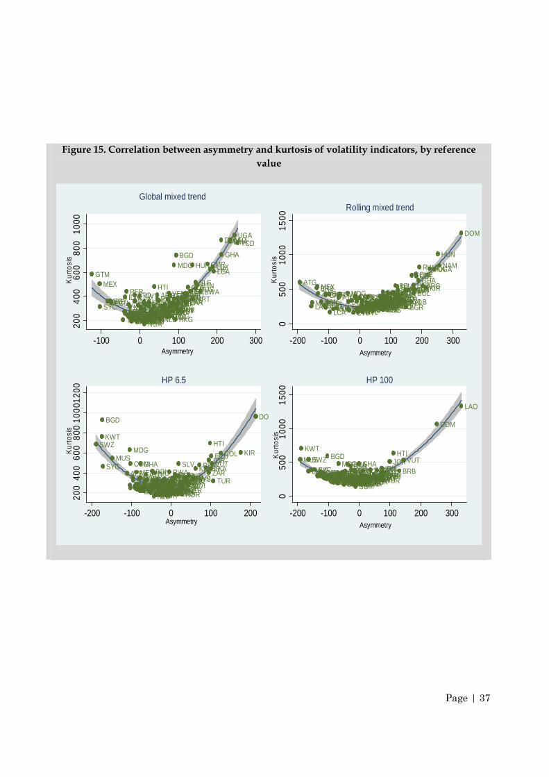
Page | 37

Figure 15. Correlation between asymmetry and kurtosis of volatility indicators, by reference

value

AGO

ALBAREARG

ATG

AUS

AUTBDI

BELBEN BFA

BGD

BGRBHRBLZ

BOL

BRABRB

BTNBWA

CAFCAN

CHE

CHLCHNCIV

CMR

COG

COL

COM

CRI

CYP

DEU

DMA

DNK

DOM

DZAECUEGY

ESPETHFINFJI

FRAGABGBR

GHA

GMBGNBGRC

GTM

GUY

HKGHND

HTI

HUN

IDN

IND

IRLIRNISL

ISRITA

JAMJORJPNKEN KIR

KNAKORKWT

LAO

LCA

LKA

LSO

LUX

MAC

MAR

MDG

MEX

MLIMLT

MOZ

MRTMUS

MWIMYS

NAMNER

NGA

NIC

NLDNOR

NPLNZL

OMNPAK

PAN

PER

PHL PNGPRI PRTPRY

RWA

SAU

SEN

SLB

SLE

SLV

SOMSTPSURSWESWZSYC

SYR

TCD

TGO THATON

TTO

TUN

TUR

UGA

URY USAVCT

VEN VUTZAF ZARZMBZWE

200

400

600

800

1000

-100 0 100 200 300Asymmetry

Global mixed trend

Kur

tosi

s

AGOALBARE

ARGATG

AUSAUTBDI

BEL

BENBFA BGDBGR

BHR

BLZ

BOL

BRA

BRB

BTNBWA

CAF

CAN

CHE

CHLCHNCIV

CMRCOG

COL

COMCRICYP

DEU

DMA

DNK

DOM

DZA

ECUEGYESP

ETHFINFJI

FRAGAB

GBR

GHA

GMB

GNBGRC

GTMGUYHKGHND HTI

HUN

IDN

INDIRLIRN

ISLISR

ITA JAMJOR

JPNKEN

KIR

KNA KORKWT

LAOLCA

LKA

LSO

LUX

MACMAR

MDGMEX

MLIMLT

MOZMRTMUS MWI

MYS

NAM

NER NGANICNLD

NORNPL NZL

OMNPAKPANPERPHL

PNGPRIPRT

PRY

RWA

SAU

SEN

SLB SLESLVSOMSTP

SURSWESWZ

SYC

SYR TCDTGOTHA

TONTTO

TUN

TURUGA

URYUSAVCTVEN

VUT

ZAFZARZMBZWE

050

010

0015

00

-200 -100 0 100 200 300Asymmetry

Rolling mixed trend

Kur

tosi

s

AGOALB

AREARGATG

AUSAUT

BDI

BELBEN BFA

BGD

BGRBHR

BLZ BOLBRA

BRBBTNBWA

CAFCANCHECHL

CHNCIV

CMRCOG

COLCOM

CRICYP

DEUDMADNK

DOM

DZA

ECU

EGY

ESPETH

FINFJIFRAGABGBR

GHA

GMBGNBGRC

GTMGUYHKG

HND

HTI

HUNIDN IND

IRL

IRNISL

ISR

ITAJAM

JOR

JPN

KEN

KIR

KNAKOR

KWT

LAOLCA

LKA

LSOLUX

MAC MAR

MDG

MEXMLI

MLTMOZ

MRT

MUS

MWIMYS

NAM NERNGA

NIC

NLD NORNPL

NZLOMN

PAKPAN

PER

PHLPNGPRIPRTPRY

RWA

SAUSEN

SLBSLESLV

SOM STPSUR

SWE

SWZ

SYC

SYRTCD

TGOTHATON

TTOTUN

TURUGA URYUSA VCT

VEN

VUT

ZAF

ZARZMB

ZWE

200

400

600

800

1000

1200

-200 -100 0 100 200Asymmetry

HP 6.5

Kur

tosi

s

AGOALBARE ARGATGAUSAUT BDIBEL BEN BFA

BGD

BGRBHR

BLZ BOLBRA

BRBBTNBWA

CAF CANCHE

CHL CHNCIV CMRCOG

COLCOMCRI

CYPDEU DMADNK

DOM

DZA

ECUEGYESP ETH

FINFJIFRA

GABGBR

GHA

GMBGNBGRC

GTMGUYHKG HND

HTI

HUNIDN IND

IRL

IRNISL

ISRITA JAM

JOR

JPNKEN KIRKNA

KOR

KWT

LAO

LCA LKALSOLUX MAC

MAR

MDG

MEXMLIMLT

MOZ MRT

MUS

MWIMYSNAMNERNGA

NICNLD NORNPL NZLOMNPAKPAN

PERPHLPNG

PRIPRT PRY

RWA

SAU SENSLB SLESLV

SOMSTPSUR

SWE

SWZSYC

SYRTCD

TGOTHA TON

TTOTUN

TURUGAURY

USA VCTVEN

VUT

ZAFZARZMBZWE

050

010

0015

00

-200 -100 0 100 200 300Asymmetry

HP 100

Kur

tosi

s

Page | 38

Conclusion

The aim of this article is to review the research into macroeconomic volatility along with an analysis

of the usual indicators of volatility. The literature on the subject, although very extensive, uses a

diverse range of volatility indicators. The techniques used vary in terms of the choice of reference

value and the way in which deviations from the reference value are calculated. Although, in general,

the research is limited to examining the magnitude of volatility, it is possible to extend the analysis

to the effects of the asymmetry of shocks and the occurrence of extreme deviations. In fact, both of

these aspects are separate dimensions of volatility but largely ignored in the literature on the

subject.

Moreover, we have limited our analysis to indicators designed to reflect the transitory variations –

both certain and uncertain – in export revenues. Measuring the uncertainty resulting from the

fluctuations of an economic variable requires the use of specific statistical tools, which have not been

addressed in this paper. We have suggested four possible methods for calculating a reference value.

The first two involve predicting the change in exports based on a mixed trend, including a

deterministic and a random component. This method is reliant on selecting an appropriate

functional form. Although observing the behaviour of the series for each country can be time-

consuming when working on panel data, a thorough review of the literature on the order of

integration of the variable concerned, combined with a spectrum analysis and the use of unit root

tests can provide us with useful information on specifying an appropriate functional form.

Moreover, in our view it is better to opt for a rolling estimated trend than a “global” mixed trend,

since it enables the coefficients estimated to vary over time and reflects recent changes in the trend

of the series more accurately.

A filtering approach has the advantage of not being based on an a priori formalisation of the change

in the series. It also offers the advantage of being sensitive to breaks in the trend over time.

Problems of leakage or compression can nevertheless introduce/exclude undesirable/relevant

components in order to study the effects of short-term fluctuations. Applied to developing

countries, the choice of a smoothing parameter between 6 and 10 initially appears preferable, since

the trend in these countries seems to fluctuate more significantly.

We have also set out the various possibilities for calculating deviations and the various effects the

latter are assumed to reflect. We have drawn a distinction between the magnitude of volatility –

measured by an indicator of average dispersion around the reference value, asymmetry – measured

by the coefficient of asymmetry for the distribution of deviations, and the occurrence of the extreme

values of deviations – measured by the kurtosis of the distribution of deviations. Whilst the

indicators for the magnitude of volatility obtained from the various reference values are very

strongly correlated, this is not the case for measures of asymmetry and kurtosis. It thus appears that

every moment in the distribution of deviations around the reference values expresses a particular

aspect of volatility. The coefficient of asymmetry seems particularly interesting because of its

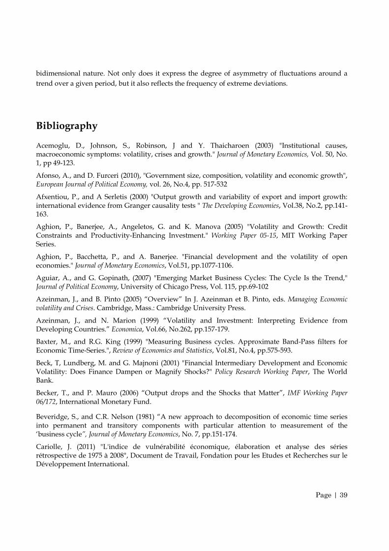
Page | 39

bidimensional nature. Not only does it express the degree of asymmetry of fluctuations around a

trend over a given period, but it also reflects the frequency of extreme deviations.

Bibliography

Acemoglu, D., Johnson, S., Robinson, J and Y. Thaicharoen (2003) "Institutional causes, macroeconomic symptoms: volatility, crises and growth." Journal of Monetary Economics, Vol. 50, No. 1, pp 49-123.

Afonso, A., and D. Furceri (2010), "Government size, composition, volatility and economic growth", European Journal of Political Economy, vol. 26, No.4, pp. 517-532

Afxentiou, P., and A Serletis (2000) "Output growth and variability of export and import growth: international evidence from Granger causality tests " The Developing Economies, Vol.38, No.2, pp.141-163.

Aghion, P., Banerjee, A., Angeletos, G. and K. Manova (2005) "Volatility and Growth: Credit Constraints and Productivity-Enhancing Investment." Working Paper 05-15, MIT Working Paper Series.

Aghion, P., Bacchetta, P., and A. Banerjee. "Financial development and the volatility of open economies." Journal of Monetary Economics, Vol.51, pp.1077-1106.

Aguiar, A., and G. Gopinath, (2007) "Emerging Market Business Cycles: The Cycle Is the Trend," Journal of Political Economy, University of Chicago Press, Vol. 115, pp.69-102

Azeinman, J., and B. Pinto (2005) “Overview” In J. Azeinman et B. Pinto, eds. Managing Economic volatility and Crises. Cambridge, Mass.: Cambridge University Press.

Azeinman, J., and N. Marion (1999) “Volatility and Investment: Interpreting Evidence from Developing Countries.” Economica, Vol.66, No.262, pp.157-179.

Baxter, M., and R.G. King (1999) "Measuring Business cycles. Approximate Band-Pass filters for Economic Time-Series.", Review of Economics and Statistics, Vol.81, No.4, pp.575-593.

Beck, T, Lundberg, M. and G. Majnoni (2001) "Financial Intermediary Development and Economic Volatility: Does Finance Dampen or Magnify Shocks?" Policy Research Working Paper, The World Bank.

Becker, T., and P. Mauro (2006) “Output drops and the Shocks that Matter”, IMF Working Paper 06/172, International Monetary Fund.

Beveridge, S., and C.R. Nelson (1981) “A new approach to decomposition of economic time series into permanent and transitory components with particular attention to measurement of the ‘business cycle”, Journal of Monetary Economics, No. 7, pp.151-174.

Cariolle, J. (2011) "L'indice de vulnérabilité économique, élaboration et analyse des séries rétrospective de 1975 à 2008", Document de Travail, Fondation pour les Etudes et Recherches sur le Développement International.

Page | 40

Chauvet, L, and P. Guillaumont (2007) "Aid, Volatility and Growth Again." Etudes et documents, Centre d’Etudes et de Recherches sur le Développement International.

Cogley, T., and J. Nason (1995) "Effects of the Hodrick-Prescott filter on trend and difference stationary time series Implications for business cycle research" Journal of Economic Dynamics and Control, Vol.19, pp. 253-278.

Combes, J.L., and P. Guillaumont. (2002) "Commodity Price Volatility, Vulnerability and Development." Development Policy Review.

Combes, J.L., Guillaumont, P., Guillaumont-Jeanneney,S., and P. Combes. (2000) "Ouverture sur l’extérieur et instabilité des taux de croissance." Revue Française d’Economie, Vol.15, No.1, pp3-33.

Dawe, D. (1996) “A New Look at the Effects of Export Volatility on Investment and Growth”, World Development, Vol.24, No.12, pp.1905-1914.

Dehn, J. (2000) “Commodity Price Uncertainty in Developing Countries”, Policy Research Working Paper 2426, The World Bank.

Dehn, J, Gilbert, C.L., and P. Varangis (2005) “Agricultural commodity price volatility” In J. Azeinman et B. Pinto, eds. Managing Economic volatility and Crises. Cambridge, Mass.: Cambridge University Press, 2005.

Di Giovanni, J., and A.A. Levchenko (2010) “The Risk Content of Exports: a Portfolio view of International trade”, Working Paper Series No. 16005, NBER.

Easterly, W., Kremer, M., Pritchett, L and L.H. Summers (1993) "Good policy or good luck?: Country growth performance and temporary shocks." Journal of Monetary Economics Vol.32, No. 3, pp.459-483.

Chris Elbers & Jan Willem Gunning & Bill Kinsey (2007) "Growth and Risk: Methodology and Micro Evidence," World Bank Economic Review, Oxford University Press, vol. 21(1), pages 1-20.

Fatás, A, and I. Mihov (2005) "Policy Volatility, Institutions and Economic Growth." Working Paper 5388, Centre for Economic Policy Research.

Fatas, A, and I. Mihov “Fiscal Discipline, Volatility, and Growth”, in Fiscal Policy, Stabilization, and Growth, eds. Perry G., Servén, L., and R. Suescun, Latin American Development Forum, The World Bank, 2007.

Gelb, A., H. (1979) "On the Definition and Measurement of Volatility and the Costs of Buffering Export Fluctuations", The Review of Economic Studies, Vol. 46, No 1 , pp.149-162.

Ghirmay, T., Sharma, S., and R. Grabowski (1999) "Export volatility, income terms of trade volatility and growth: causal analyses." The Journal of International Trade & Economic Development, Vol.8, No.2, pp.209 - 229.

Gorard, S. (2005) “Revisiting the 90-year-old Debate: the Advantage of the Mean Deviation”, British Journal of Educational Studies, Vol.53, No.4, pp.417-430.

Guay, A., and P. St-Amant, (1997). "Do the Hodrick-Prescott and Baxter-King Filters Provide a Good Approximation of Business Cycles?," Cahiers de recherche CREFE / CREFE Working Papers 53, CREFE, Université du Québec à Montréal.

Guillaumont, P. (2010) “Assessing the Economic Vulnerability of Small Island Developing States and the Least Developed Countries”, Journal of Development Studies, Vol.46, No.5, pp.828-854.

Page | 41

Guillaumont, P., Caught in a trap: Identifying the Least Developed Countries. Economica. October 2009.

Guillaumont, P. (2009) “An Economic Vulnerability Index: Its Design and Use for International Development Policy”, Oxford Development Studies, Volume 37, No.3, pp.193-228.

Guillaumont, P. (2007) “Economic vulnerability, persistent challenge to African development” Revue Africaine du Développement, Vol.19, No.1, pp.123-162.

Guillaumont, P. (2007) “A Retrospective EVI : Methodological Aspects” Etudes et Documents, CERDI, E 2007.15.

Guillaumont, P., Guillaumont-Jeanneney, S., and J.F. Brun (1999) “How volatility lowers African growth.” Journal of African Economies, Vol.8, No.1, pp.87-107.

Hnatkovska, V. (2005) “Appendix.” In J. Azeinman and B. Pinto, eds. Managing Economic volatility and Crises. Cambridge, Mass.: Cambridge University Press.

Hnatkovska, V., and N. Loayza (2005) “Volatility and Growth.” In J. Azeinman and B. Pinto, eds. Managing Economic volatility and Crises. Cambridge, Mass.: Cambridge University Press.

Hodrick, R., and E. Prescott (1997) "Postwar US Business Cycles: An Empirical Investigation."Journal of Money, Credit and Banking, Blackwell Publishing, Vol. 29, No.1, pp. 1-16.

Hurlin C., and V. Mignon (2005) "Une synthèse des tests de racine unitaire sur données de panel", Économie et Prévision, no. 169-170 ,pp. 253-294.

Imbs, J. (2007) “Growth and Volatility”, Journal of Monetary Economics, Vol.54, No.7, pp.1848-1862.

King, R., and S. Rebelo (1993) "Low Frequency Filtering and Real Business Cycles." Journal of Economic Dynamics and Control, Vol.17, No. 2, pp.207-231.

Konya, L. (2004) "Unit-Root, Co-integration and Granger Causality Test Results for Export and Growth in OECD Countries."International Journal of Applied Econometrics and Quantitative Studies, Vol. 1, No. 2, pp.67-94.

Koren, M. and S. Tenreyro (2007) “Volatility and Development”, Quarterly Journal of Economics, Vol.122, No.1, pp.243-287.

Koren, M., and S. Tenreyro (2006) "The Growth and Welfare Effects of Macroeconomic Volatility." Working Paper, Centre for Economic Policy Research.

Lensink, R., and O. Morrissey (2006) "Foreign Direct Investment: Flows, Volatility, and the Impact on Growth." Review of International Economics, Vol.14, No.3, pp.478-493.

Loayza, NV., and C. Raddatz (2007) “The Structural Determinants of External Vulnerability”, World Bank Economic Review, Vol.21, No.3, pp.359-387.

Loayza, NV., Rancière, R., Servén, L., and J. Ventura (2007) “Macroeconomic volatility and Welfare in Developing Countries: An Introduction”, World Bank Economic Review, Vol.21, No.3, pp.343-357.

Maddala, G, and I Kim (1996) "Structural change and unit roots." Journal of Statistical Planning and Inference, Vol.49, pp.73-103.

Malik, A., and J. Temple (2009) "The Geography of output volatility", Journal of Development Economics, Vol.90, pp.163-178.

Maravall, A, and A. Del Rio (2001) "Time aggregation and the Hodrick-Prescott filter." Working Paper, No. 108.

Page | 42

Mauro, P., and T. Becker (2006) “Output Drops and the Shocks that Matter” IMF Working Papers, International Monetary Fund, WP/06/172.

Mobarak, A. (2005) "Democracy, Volatility, and Economic Development." Review of Economics and Statistics, Vol.87, No.2, pp.348-361.

Nelson, C., and C. Plosser (1982) "Trends and random walks in macroeconomic time series: Some evidence and implications." Journal of Monetary Economics, Vol.10, No.2, pp.139-162.

Nelson, C., and H. Kang (1981) "Spurious periodicity in inappropriately detrended time series." Econometrica, Vol.49, No.3, pp.741-751.

Pritchett, L. (2000) "Understanding Patterns of Economic Growth: Searching for Hills among Plateaus, Mountains, and Plains" The World Bank Economic Review, Vol.14, No.2,pp. 221-250.

van der Ploeg, F., and S. Poelhekke (2009) "Volatility and the natural resource curse”, Oxford Economic Papers, Oxford University Press, vol. 61, No.4, pages 727-760.

Raddatz, C. (2007) "Are external shocks responsible for the volatility of output in low-income countries?" Journal of Development Economics, Vol.84, No.1, pp.155-187.

Ramey, G., and V.A. Ramey (1995) "Cross-country Evidence on the Link Between Volatility and Growth." The American Economic Review Vol.85, No. 5, pp.1138-1151.

Rancière, R., Tornell, A., and F. Westermann (2008) “Systemic crises and growth”, Quarterly Journal of Economics, Vol.123, No.1, pp.359-406.

Rand, J., and F. Tarp (2002) "Business Cycles in Developing Countries: Are They Different?" World Development, Vol. 30, No.12, pp.2071-2088.

Rodrik, D. (2000) “Participatory Politics, Social Cooperation, and Economic Stability”, The American Economic Review, Vol.90, No.2, pp.140-144.

Rodrik, D. (1998) “Why Do Open Economies Have Bigger Governments?”, Journal of Political Economy, Vol.106, No.5, pp.997-1032.

Serven, L. (1998) "Macroeconomic Uncertainty and Private Investment in Developing Countries: An Empirical Investigation." Policy Research Working Paper, The World Bank.

Serven, L. (1997) "Uncertainty, Volatility, and Irreversible Investment: Theory, Evidence, and Lessons for Africa." Journal of African Economies, Vol.6, No.3, pp.229-268.

Tsui, K., Y., (1988) "The measurement of exports volatility – a methodological note", Economics Letters Vol.27, No 1, pp.61-65.

Van der Ploeg, F., and S. Poelheeke (2009) “Volatility and the Natural Resource Curse”. Oxford Economic Papers, Vol. 61, No.4, pp. 727-760

Van Norden, S. (2004) “Filtres pour l’analyse courante”, L’Actualité Economique, Vol. 80, No.2-3 pp.523-546.

Wolf, H. (2005) “Volatility: Definitions and Consequences.” In J. Azeinman and B. Pinto, eds. Managing Economic volatility and Crises. Cambridge, Mass.: Cambridge University Press, 2005.

Page | 43

Appendices

Page | 44

Appendix A.1 Overview of indicators of volatility and their application in the literature.

Indicators Authors Phenomenon Variables concerned (yt) G

row

th r

ate

/fir

st d

iffe

ren

ce

Standard deviation or coefficient of variation of growth rate

Servén (1997), Acemoglu et al. (2003), Mobarak (2005), Koren and Tenreyro (2006), Raddatz (2007), Di Giovanni and Levchenko (2007), Malik and Temple (2009), Ploeg and Poelhekke (2009)

Variability

GDP/inhabitant, inflation, terms of trade, actual exchange rate, black-market premium, international interest rate (LIBOR), development aid/inhabitant, public spending, ratio of wheat cultivation yields to national yield

Variance of growth rate over five years Koren and Tenreyro (2006) variability Annual growth rate of work productivity

Fil

ters

Decline in GDP: decrease of more than 1% of the (annual) series log smoothed by the HP filter (lambda=1000)

Mauro and Becker (2006) Variability GDP

Standard deviation of the cyclical component, i.e. the standard deviation of the difference between series smoothed by the HP or BK filter and actual series.

Hnatkovska and Loayza (2005); Guillaumont and Chauvet (2007), Afonso and Furceri (2010)

Variability Aid, export revenues, GDP.

Variability GDP, budget variables

(transfers, subsidies, public spending, tax revenues, etc.)

Page | 45

Average over five years of the ratio of the absolute deviation between the observed value of export revenues (X) and the value filtered using a moving average process over five years, based on GDP (Y):

INST = 1

T − 4

X j − 15

X k

k = j − 2

j + 2

∑

Y jj = 3

T − 2

∑

Dawe (1996) Variability Export revenues

Fo

reca

sts/

Est

ima

tes

initialit

initialitititit popIyydummyttty δλγβϕαααα +++++++++=∆ −− 21197419743

2210

The standard deviation of the residual itε, is seen as a measure of

volatility reflecting uncertainty. This approach is adopted for the whole of the sample and for all countries, to produce an estimate of coefficients specific to each country.

Ramey and Ramey (1995) Uncertainty Growth rate of GDP

The standard deviation of the residual tε, obtained using a regression of

yt on a linear trend:

tt ty εβα ++=

Pritchett (2000), Mobarak (2005) Variability Growth rate of GDP per inhabitant, growth rate of capital per worker

Rolling standard deviation or average absolute deviation of the residual

tεobtained based on a regression of yt on a rolling mixed trend,

y t = α + β t + γy t −1 + ε t

Guillaumont and Combes (2002), Guillaumont and Chauvet (2007), Servén (1998)

Variability/uncertainty

Development aid, exports, terms of trade, inflation rate, relative price of capital, actual exchange rate, growth rate of GDP.

Standard deviation of the error in a regression of FDI over three lags and a temporal trend:

y t = α + β t + γ 1y t −1 + γ 2 y t − 2 + γ 3 y t − 3 + ε t

Lensink and Morrissey (2006)

Uncertainty FDI/GDP, FDI

They estimate volatility measures for each country based on the following GARCH(1,1) model:

∆ y it = α 0 + α 1t + α 2 t 2 + β 1∆ y it −1 + β 2 y it − 2 + δ D t + ε it

where t=1…,T and D the vector of mute quarterly variables.

By imposing the following constraint on conditional variance

σ it2 = γ i , 0 + γ i ,1ε i , t − 1

2 + δ iσ it − 12

The estimated value of itσ represents the uncertainty of yit.

Dehn (2000), Servén (1998) and Afxentiou and Serletis (2000)

Uncertainty

Prices of raw materials, inflation rate, price of capital relative to actual exchange rate

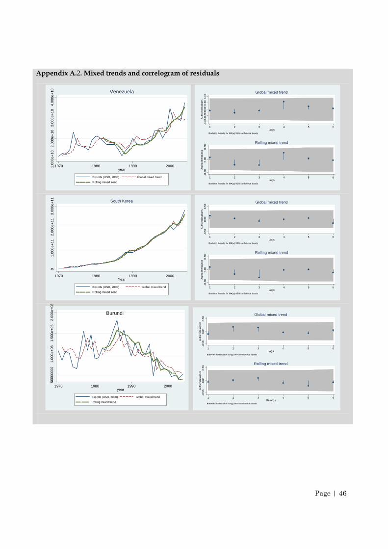
Page | 46

Appendix A.2. Mixed trends and correlogram of residuals

1.00

0e+

102.

000e

+10

3.00

0e+

104.

000e

+10

1970 1980 1990 2000year

Exports (USD, 2000) Global mixed trend

Rolling mixed trend

Venezuela

-0.4

0-0

.20

0.00

0.20

0.40

Aut

ocor

rela

tions

1 2 3 4 5 6Lags

Bartlett's formula for MA(q) 95% confidence bands

Global mixed trend

-0.5

00.

000.

50A

utoc

orre

latio

ns

1 2 3 4 5 6Lags

Bartlett's formula for MA(q) 95% confidence bands

Rolling mixed trend

01.

000e

+11

2.00

0e+

113.

000e

+11

1970 1980 1990 2000Year

Exports (USD, 2000) Global mixed trend

Rolling mixed trend

South Korea-0

.50

0.00

0.50

Aut

ocor

rela

tions

1 2 3 4 5 6Lags

Bartlett's formula for MA(q) 95% confidence bands

Global mixed trend-0

.50

0.00

0.50

Aut

ocor

rela

tions

1 2 3 4 5 6Lags

Bartlett's formula for MA(q) 95% confidence bands

Rolling mixed trend

Burundi

500

0000

01.

000

e+08

1.5

00e+

082

.000

e+08

1970 1980 1990 2000year

Exports (USD, 2000) Global mixed trend

Rolling mixed trend

-0.5

00.

000.

50A

utoc

orre

latio

ns

1 2 3 4 5 6Lags

Bartlett's formula for MA(q) 95% confidence bands

Global mixed trend

-0.5

00.

000.

50A

utoc

orre

latio

ns

1 2 3 4 5 6Retards

Bartlett's formula for MA(q) 95% confidence bands

Rolling mixed trend

Page | 47

2.00

0e+

093.

000e

+09

4.00

0e+

09

1970 1980 1990 2000year

Exports (USD, 2000) Global mixed trend

Rolling mixed trend

Kenya

-0.4

0-0

.20

0.00

0.20

0.40

Aut

ocor

rela

tions

1 2 3 4 5 6Lags

Bartlett's formula for MA(q) 95% confidence bands

Global mixed trend

-0.5

00.

000.

50A

utoc

orre

latio

ns

1 2 3 4 5 6Lags

Bartlett's formula for MA(q) 95% confidence bands

Rolling mixed trend

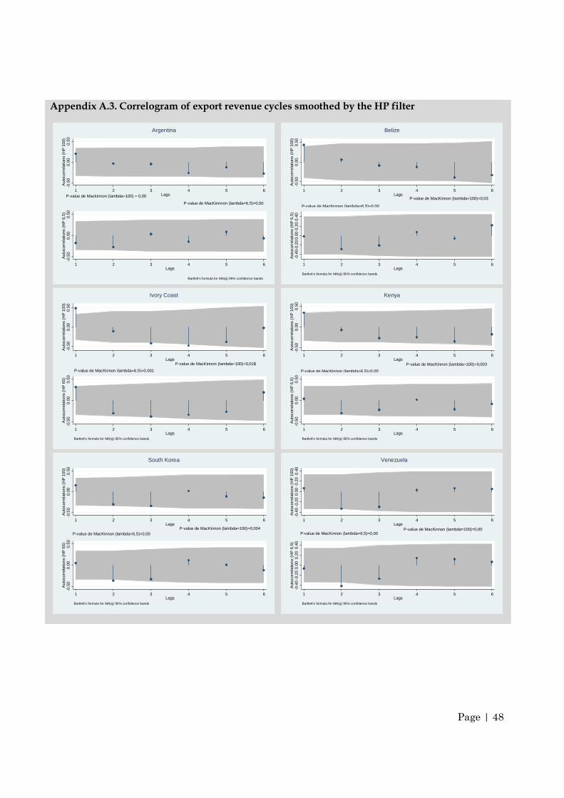
Page | 48

Appendix A.3. Correlogram of export revenue cycles smoothed by the HP filter

-0.5

00.

000.

50A

utoc

orre

latio

ns (

HP

100

)

1 2 3 4 5 6LagsP-value de Mackinnon (lambda=100) = 0,00

P-value de MacKinnnon (lambda=6,5)=0,00

-0.5

00.

000.

50A

utoc

orre

latio

ns (

HP

6,5

)

1 2 3 4 5 6Lags

Bartlett's formula for MA(q) 95% confidence bands

Argentina

-0.5

00.

000.

50A

utoc

orre

latio

ns (

HP

100

)

1 2 3 4 5 6Lags

P-value de MacKinnon (lambda=100)=0,03

P-value de MacKinnon (lambda=6,5)=0,00

-0.4

0-0.

200.

000.

200.

40A

utoc

orre

latio

ns (

HP

6,5

)

1 2 3 4 5 6Lags

Bartlett's formula for MA(q) 95% confidence bands

Belize

-0.5

00.

000.

50A

utoc

orre

latio

ns (

HP

100

)

1 2 3 4 5 6Lags

P-value de MacKinnon (lambda=100)=0,01$

P-value de MacKinnon (lambda=6,5)=0,001

-0.5

00.

000.

50A

utoc

orre

latio

ns (

HP

65)

1 2 3 4 5 6Lags

Bartlett's formula for MA(q) 95% confidence bands

Ivory Coast-0

.50

0.00

0.50

Aut

ocor

rela

tions

(H

P 1

00)

1 2 3 4 5 6Lags

P-value de MacKinnon (lambda=100)=0,003

P-value de MacKinnon (lambda=6,5)=0,00

-0.5

00.

000.

50A

utoc

orre

latio

ns (

HP

6,5

)

1 2 3 4 5 6Lags

Bartlett's formula for MA(q) 95% confidence bands

Kenya

-0.5

00.

000.

50A

utoc

orre

latio

ns (

HP

100

)

1 2 3 4 5 6Lags

P-value de MacKinnon (lambda=100)=0,004P-value de MacKinnon (lambda=6,5)=0,00

-0.5

00.

000.

50A

utoc

orre

latio

ns (

HP

65)

1 2 3 4 5 6Lags

Bartlett's formula for MA(q) 95% confidence bands

South Korea

-0.4

0-0

.20

0.00

0.20

0.40

Aut

ocor

rela

tions

(H

P 1

00)

1 2 3 4 5 6Lags

P-value de MacKinnon (lambda=100)=0,00P-value de MacKinnon (lambda=6,5)=0,00

-0.4

0-0

.20

0.00

0.20

0.40

Aut

ocor

rela

tions

(H

P 6

,5)

1 2 3 4 5 6Lags

Bartlett's formula for MA(q) 95% confidence bands

Venezuela

Page | 49

Appendix A.4 Comparative evolution of deviations (in % of trend values)

-40

-20

02

040

60

in %

of t

rend

1970 1980 1990 2000Year

Rolling mixed trend Global mixed trend

HP 6.5 HP 100

Argentina

-.2

0.2

.4

1980 1985 1990 1995 2000 2005year

Rolling mixed trend Global mixed trend

HP 6.5 HP 100

Belize

in %

of t

ren

d

-.6

-.4

-.2

0.2

.4

1970 1980 1990 2000year

Rolling mixed trend Global mixed trend

HP 6.5 HP 100

Burundi

in %

of t

rend

-.2

-.1

0.1

.2.3

1970 1980 1990 2000year

Rolling mixed trend Global mixed trend

HP 6.5 HP 100

Ivory Coast

in %

of t

rend

-.2

0.2

.4.6

1970 1980 1990 2000year

Global mixed trend Rolling mixed trend

HP 6.5 HP 100

South Korea

in %

of t

ren

d

-.4

-.2

0.2

.4.6

1970 1980 1990 2000year

Global mixed trend Rolling mixed trend

HP 6.5 HP 100

Venezuela

in %

of t

rend