Embed Size (px)
Citation preview

JOURNAL OF CHEMICAL PHYSICS VOLUME 111, NUMBER 4 22 JULY 1999
One-dimensional arrays of oscillators: Energy localizationin thermal equilibrium
Ramon Reigadaa)
Department of Chemistry and Biochemistry 0340, University of California San Diego,La Jolla, California 92093-0340
Aldo H. Romerob)
Department of Chemistry and Biochemistry 0340, and Department of Physics, University of California,San Diego, La Jolla, California 92093-0340
Antonio Sarmientoc)
Department of Chemistry and Biochemistry 0340, University of California San Diego,La Jolla, California 92093-0340
Katja LindenbergDepartment of Chemistry and Biochemistry 0340, and Institute for Nonlinear Science,University of California San Diego, La Jolla, California 92093-0340
~Received 4 March 1999; accepted 29 April 1999!
All systems in thermal equilibrium exhibit a spatially variable energy landscape due to thermalfluctuations. Thus at any instant there is naturally a thermodynamically driven localization of energyin parts of the system relative to other parts of the system. The specific characteristics of the spatiallandscape such as, for example, the energy variance, depend on the thermodynamic properties of thesystem and vary from one system to another. The temporal persistence of a given energy landscape,that is, the way in which energy fluctuations~high or low! decay toward the thermal mean, dependson the dynamical features of the system. We discuss the spatial and temporal characteristics ofspontaneous energy localization in 1D anharmonic chains in thermal equilibrium. ©1999American Institute of Physics.@S0021-9606~99!51628-0#
llaa
asrg
ect.e
arpam
ica
inhe-lso
gyem
r-atic,ath-
tantthein
beof
ces.icha-en
her-ned-s ofical
s,be-
erto
ofmenearis
-
-
d
I. INTRODUCTION
The pioneering work of Fermi, Pasta, and Ulam1 dem-onstrated that a periodic lattice of coupled nonlinear oscitors is not ergodic, and that energy in such a lattice mnever be distributed uniformly. A great deal of work hfollowed that classic paper trying to understand how eneis distributed in discrete nonlinear systems.2–7 Specifically,the possibility of spontaneous energy localization in perfanharmonic lattices has been a subject of intense interes8–13
The existence of solitons and more generally of breathand other energy-focusing mechanisms, and the stationor periodic recurrence or even slow relaxation of such stially localized excitations, are viewed as nonlinear phenoena with important consequences in many physsystems.10,14,15
The interest in the distribution and motion of energyperfect arrays arises in part because localized energy in tsystems may bemobile, in contrast with systems where energy localization occurs through disorder. The interest aarises because such arrays may themselves serve as mfor a heat bath for other systems connected to them.16 Albeitin different contexts, ‘‘perfect’’ arrays serving as enerstorage and transfer assemblies for chemical or photochcal processes are not uncommon.17,18
a!Permanent address: Departament de Quı´mica-Fısica, Universitat de Barcelona, Avda. Diagonal 647, 08028 Barcelona, Spain.
b!Present address: Max-Planck Institut fu¨r Festkorperforschung, Heisenbergstr. 1, 70569 Stuttgart, Germany.
c!Permanent address: Instituto de Astronomı´a, Apdo. Postal 70-264, CiudaUniversitaria, Me´xico D. F. 04510, Me´xico.
1370021-9606/99/111(4)/1373/12/$15.00
-y
y
t
rsity--l
se
odels
i-
The study of anharmonic chains and of highedimensional discrete arrays has been less than systemcertainly an inevitable consequence of the breadth and mematical difficulty of the subject. Some studies~including thework of Fermi, Pasta, and Ulam! deal with microcanonicalarrays. Here one observes the way in which a given consamount of energy distributes itself among the elements ofarray. The notion of ‘‘temperature’’ usually does not enterthese discussions, although such an association couldmade if the energy is randomly distributed. Other studiesanharmonic chains~far more limited in number! deal withsystems subject to external noise and other external forThe questions of interest here involve the ways in whnoise can enhance~as in noise-enhanced signal propgation!15 or even totally modify~as in noise-induced phastransitions!19 the properties of the nonlinear array. Evemore limited has been the study of systems that are in tmal contact with one or more external heat baths maintaiat a constant temperature.10,12 Here the questions usually revolve around the robustness against thermal fluctuationstationary or quasistationary solutions of the microcanonproblem. In both microcanonical and canonical systemsome work concentrates on stationary states or long-timehavior or equilibrium properties of the array, while othwork deals with transport properties or with the approachequilibrium. Furthermore, there is variation in the portionthe potential where the nonlinearity resides. Thus, in socases the elements of the array are themselves nonliwhile in others it is the coupling between elements thatnonlinear~and, on occasion, both are nonlinear!.
3 © 1999 American Institute of Physics
o-s-estiata
ean-ec
Wc
thoytos
teexnga
th
d
of
e
-ic
ano
byndee
Oaiin
mesase
on
w
n-
hisds,
hat
b--
tor
en any
on?ana-in
lede-t
in-r in
i-
rsis-agyn-r-
ex-he
tua-tor
caning
ofon
os-os-erengeen-
onthis
o-terour
softndalled,’’lo-or
1374 J. Chem. Phys., Vol. 111, No. 4, 22 July 1999 Reigada et al.
Within this broad setting, our interest in this paper fcuses on one-dimensional arrays of classical oscillatorthermal equilibrium.12 An understanding of thermal equilibrium properties and the effects of nonlinearities on thproperties is a prerequisite to the perhaps more interesanalysis of the nonequilibrium behavior of anharmonic ltices in the presence of thermal fluctuations and the approto equilibrium in such systems. In particular, here we dwith the case of ‘‘diagonal anharmonicity,’’ that is, the nolinearity in our model is inherent within each oscillator in tharray ~representing, for example, intramolecular interations!, while the connections between oscillators~represent-ing, for example, intermolecular interactions! are ordinarylinear springs. The anharmonicity may be soft or hard.explore the conditions that lead to spontaneous energy loization in one or a few of the oscillators in the array, andtime it takes for a given energy landscape to change tdifferent landscape. One could undertake a parallel studsystems with anharmonic interactions between oscilla~‘‘off-diagonal’’ anharmonicity!. We address such systemin subsequent work.20
The energy landscape is determined by the local potial of each oscillator, and by the channels of energychange in and out of each of the oscillators. The couplibetween oscillators provide one such exchange channel,the coupling of the array with the heat bath providesother. We shall see that different arrays~soft, hard! behavevery differently in response to these channels. We broaanticipate our conclusions by revealing that~i! persistent en-ergy localization occurs in arrays of weakly coupled soscillators even when strongly coupled to a heat bath~whilesuch localization is absent in the hard chain!; ~ii ! persistentlocalization occurs in strongly coupled hard arrays providthey are weakly coupled to a heat bath~while such localiza-tion is absent in the soft chain!; ~iii ! quasidispersionless mobility of localized energy requires off-diagonal anharmonity.
These remarks point to the fact that our analysis ofharmonic chains in thermal equilibrium could start from tw‘‘opposite’’ viewpoints. On the one hand, we might startanalyzing uncoupled oscillators in thermal equilibrium athen proceed to investigate what happens if we couple thoscillators to one another. This approach focuses on thetropic localization mechanism12 and the way in which thecoupling between the oscillators eventually degrades it.the other hand, we might start with a coupled isolated chfocus on energetic localization mechanisms in such a cha7
and then proceed to investigate the ways in which therfluctuations and dissipation affect such local structurSince we are explicitly interested in localization in the preence of thermal fluctuations, and since entropic effects hreceived far less attention than energetic ones, we choofollow the former approach.
No matter the sequence of our queries, since hereinterest lies mainly in understanding energy localization inonlinear discrete array inthermal equilibriumand the wayin which thermal effects depend on system parameters,pose our questions as follows:
~a! How is the energy distributed in an equilibrium no
in
eng-chl
-
eal-eainrs
n--snde
ly
t
d
-
-
sen-
nn,,
als.-veto
ura
e
linear chain at any given instant of time, and how does tdistribution depend on the anharmonicity? In other worcan one talk aboutspontaneous energy localizationin ther-mal equilibrium, and, if so, what are the mechanisms tlead to it?
~b! How do local energy fluctuations in such an equilirium array relax in a given oscillator? Are there circumstances in the equilibrium system wherein a given oscillaremains at a high level of excitation for a long time?
~c! Can local high-energy fluctuations move in somnondispersive fashion along the array? In other words, caarray in thermal equilibrium transmit long-lived high-energfluctuations~if indeed they exist! from one region of thearray to another without too much energy loss to dispersi
The answers to these questions have not been foundlytically, and are for that reason most clearly presentedcomparative fashion. Starting with an ensemble of uncouposcillators at thermal equilibrium, one knows exactly the bhavior of asingle harmonic oscillatorand can say a greadeal about the behavior of asingle anharmonic oscillatorfrom general thermodynamic considerations. Thus, forstance, the mean energy of a single harmonic oscillatothermal equilibrium at temperatureT is E5kBT(kB5Boltzmann’s constant!. This energy is on average dvided equally between kinetic and potential~a partition thatenters importantly in questions concerning landscape petence!. A simple virial analysis immediately shows thatsoft anharmonic oscillator in thermal equilibrium has energreater thankBT while a hard anharmonic oscillator has eergy smaller than kBT. Both share the property of the hamonic oscillator that the average kinetic energy iskBT/2, buttheir average potential energies differ. One also knowsactly the energy fluctuations in a harmonic oscillator: tenergy variances2 is equal tokB
2T2, and the ratio ofs to Eis therefore independent of temperature. The energy fluctions are easily determined to be greater in a soft oscillaand smaller in a hard oscillator. From these facts onearrive at rather definitive qualitative conclusions regardthe distribution and persistence of energy in ensemblessingle oscillators and the effects of the anharmonicitiesthese features.12
The situation becomes more complicated when suchcillators are connected to one another. Not only can thecillators now exchange energy with the heat bath, but thare also coupling channels whereby oscillators can exchaenergy with one another. The interplay of these variousergy exchange channels and the effects of anharmonicitythis interplay are some of the issues to be addressed inwork.
This paper is organized as follows. In Sec. II we intrduce our model and notation. We fix some of the paramevalues and briefly discuss the numerical methods used insimulations. Here we introduce the hard, harmonic, andlocal potentials to be compared. In Sec. III we review aillustrate previous results for uncoupled oscillators in thermequilibrium so as to establish the background for the coupsystems. The phenomenon of ‘‘entropic localizationwhereby ensembles of single thermalized soft oscillatorscalize and retain energy more effectively than harmonic
nfl
ur
-i-
a
l ifo
mn
Theian–
har-he
lsws
u-pa-fore-–
100. Inorchn-
e se-tua-
aofin
toto
1375J. Chem. Phys., Vol. 111, No. 4, 22 July 1999 One-dimensional arrays of oscillators
hard oscillators, is recalled. In Sec. IV we explore the cosequences of coupling our oscillators. In Sec. V we brieaddress the mobility of energy fluctuations in our systemFinally, Sec. VI summarizes our findings and anticipates fther studies.
II. THE MODEL AND NUMERICAL METHODS
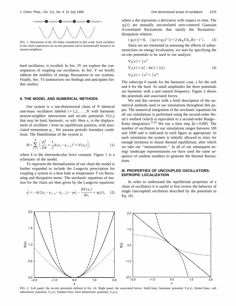
Our system is a one-dimensional chain ofN identicalunit-mass oscillators labeledi 51,2, . . . ,N with harmonicnearest-neighbor interactions and on-site potentialsV(xi)that may be hard, harmonic, or soft. Herexi is the displace-ment of oscillatori from its equilibrium position, with associated momentumpi . We assume periodic boundary condtions. The Hamiltonian of the system is
H5(i 51
N S pi2
2m1
1
2k~xi2xi 11!21V~xi ! D , ~1!
wherek is the intermolecular force constant. Figure 1 isschematic of the model.
To represent the thermalization of our chain the modefurther expanded to include the Langevin prescriptioncoupling a system to a heat bath at temperatureT via fluctu-ating and dissipative terms. The stochastic equations oftion for the chain are then given by the Langevin equatio
xi52k~2xi2xi 112xi 21!2gxi2dV~xi !
dxi1h i~ t !, ~2!
FIG. 1. Illustration of the 1D chain considered in this work. Each oscillain the chain experiences an on-site potential and is harmonically boundnearest-neighbors.
-ys.-
sr
o-s
where a dot represents a derivative with respect to time.h i(t) are mutually uncorrelated zero-centered Gaussd-correlated fluctuations that satisfy the fluctuationdissipation relation:
^h i~ t !&50, ^h i~ t !h j~ t8!&52gkBTd i j d~ t2t8!. ~3!
Since we are interested in assessing the effects of anmonicities on energy localization, we start by specifying ton-site potentials to be used in our analysis:
V0~x!5 12 x2
Vs~x!5uxu2 ln~11uxu! ~4!
Vh~x!5 12 x21 1
2 x4.
The subscript 0 stands for the harmonic case,s for the softandh for the hard. At small amplitudes the three potentiaare harmonic with a unit natural frequency. Figure 2 shothe potentials and associated forces.
We end this section with a brief description of the nmerical methods used in our simulations throughout thisper. The numerical integration of the stochastic equationsall our simulations is performed using the second-order Hun’s method~which is equivalent to a second-order RungeKutta integration!.21,22 We use a time stepDt50.005. Thenumber of oscillators in our simulations ranges betweenand 1000 and is indicated in each figure as appropriateeach simulation the system is initially allowed to relax fenough iterations to insure thermal equilibrium, after whiwe take our ‘‘measurements.’’ In all of our subsequent eergy landscape representations we have used the samquence of random numbers to generate the thermal fluctions.
III. PROPERTIES OF UNCOUPLED OSCILLATORS:ENTROPIC LOCALIZATION
In order to understand the equilibrium properties ofchain of oscillators it is useful to first review the behaviorsingle ~uncoupled! oscillators described by the potentialsEq. ~4!.
rits
FIG. 2. Left panel: the on-site potentials defined in Eq.~4!. Right panel: the associated forces. Solid lines: harmonic potential,V0(x). Dotted lines: softanharmonic potential,Vs(x). Dashed lines: hard anharmonic potential,Vh(x).
harmonic
1376 J. Chem. Phys., Vol. 111, No. 4, 22 July 1999 Reigada et al.
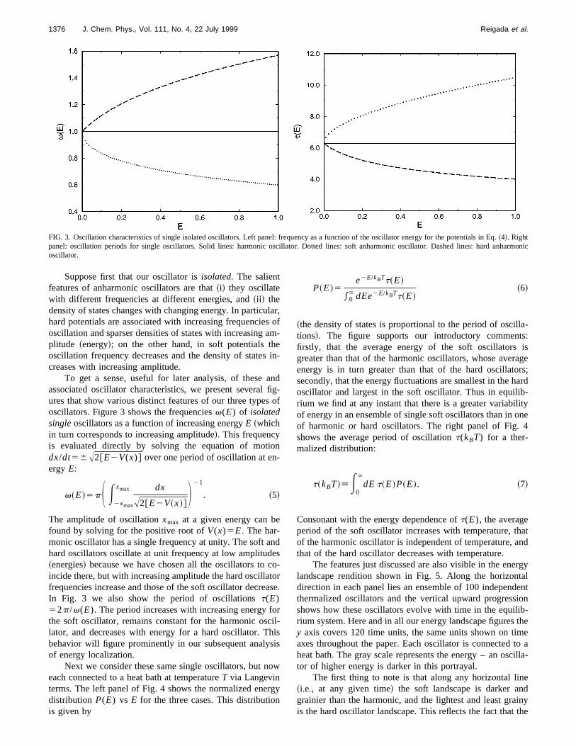
FIG. 3. Oscillation characteristics of single isolated oscillators. Left panel: frequency as a function of the oscillator energy for the potentials in Eq.~4!. Rightpanel: oscillation periods for single oscillators. Solid lines: harmonic oscillator. Dotted lines: soft anharmonic oscillator. Dashed lines: hard anoscillator.
lasame
s
anl fis
on-
e
necotoa
focih
si
o
rgn
lla-ts:is
agers;ard
b-lityne4
hatand
rgytalentionib-the
imeto acilla-
edinythe
Suppose first that our oscillator isisolated. The salientfeatures of anharmonic oscillators are that~i! they oscillatewith different frequencies at different energies, and~ii ! thedensity of states changes with changing energy. In particuhard potentials are associated with increasing frequencieoscillation and sparser densities of states with increasingplitude ~energy!; on the other hand, in soft potentials thoscillation frequency decreases and the density of statecreases with increasing amplitude.
To get a sense, useful for later analysis, of theseassociated oscillator characteristics, we present severaures that show various distinct features of our three typeoscillators. Figure 3 shows the frequenciesv(E) of isolatedsingleoscillators as a function of increasing energyE ~whichin turn corresponds to increasing amplitude!. This frequencyis evaluated directly by solving the equation of motidx/dt56A2@E2V(x)# over one period of oscillation at energy E:
v~E!5pS E2xmax
xmax dx
A2@E2V~x!#D 21
. ~5!
The amplitude of oscillationxmax at a given energy can bfound by solving for the positive root ofV(x)5E. The har-monic oscillator has a single frequency at unity. The soft ahard oscillators oscillate at unit frequency at low amplitud~energies! because we have chosen all the oscillators toincide there, but with increasing amplitude the hard oscillafrequencies increase and those of the soft oscillator decreIn Fig. 3 we also show the period of oscillationst(E)52p/v(E). The period increases with increasing energythe soft oscillator, remains constant for the harmonic oslator, and decreases with energy for a hard oscillator. Tbehavior will figure prominently in our subsequent analyof energy localization.
Next we consider these same single oscillators, but neach connected to a heat bath at temperatureT via Langevinterms. The left panel of Fig. 4 shows the normalized enedistribution P(E) vs E for the three cases. This distributiois given by
r,of-
in-
dg-of
ds-rse.
rl-iss
w
y
P~E!5e2E/kBTt~E!
*0` dEe2E/kBTt~E!
~6!
~the density of states is proportional to the period of oscitions!. The figure supports our introductory commenfirstly, that the average energy of the soft oscillatorsgreater than that of the harmonic oscillators, whose averenergy is in turn greater than that of the hard oscillatosecondly, that the energy fluctuations are smallest in the hoscillator and largest in the soft oscillator. Thus in equilirium we find at any instant that there is a greater variabiof energy in an ensemble of single soft oscillators than in oof harmonic or hard oscillators. The right panel of Fig.shows the average period of oscillationt(kBT) for a ther-malized distribution:
t~kBT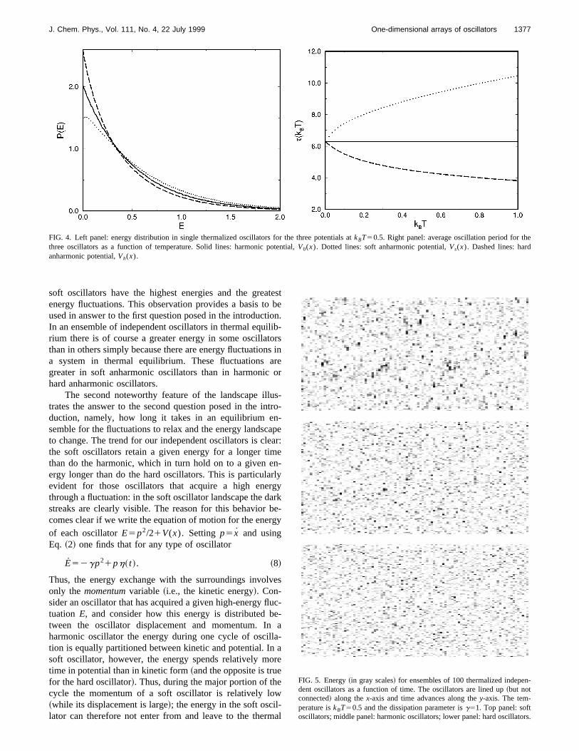
e
1377J. Chem. Phys., Vol. 111, No. 4, 22 July 1999 One-dimensional arrays of oscillators
FIG. 4. Left panel: energy distribution in single thermalized oscillators for the three potentials atkBT50.5. Right panel: average oscillation period for ththree oscillators as a function of temperature. Solid lines: harmonic potential,V0(x). Dotted lines: soft anharmonic potential,Vs(x). Dashed lines: hardanharmonic potential,Vh(x).
tb
ioilibtos
aro
usntn-a
eamnrlrgabrg
ve
ue
la
or
ew-m
n-
ors.
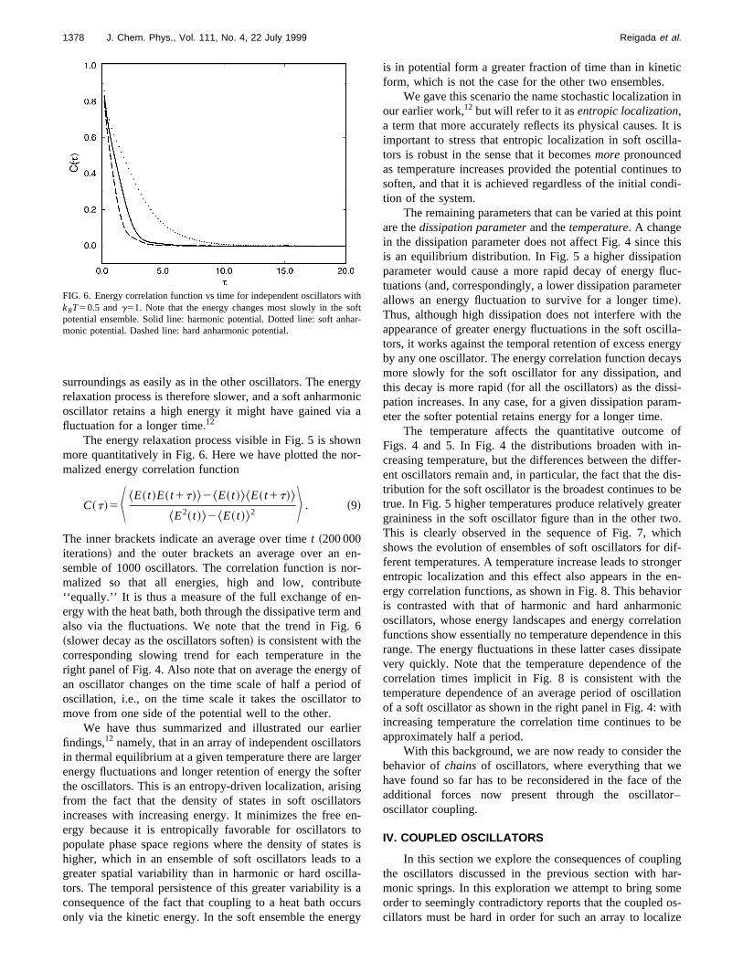
soft oscillators have the highest energies and the greaenergy fluctuations. This observation provides a basis toused in answer to the first question posed in the introductIn an ensemble of independent oscillators in thermal equrium there is of course a greater energy in some oscillathan in others simply because there are energy fluctuationa system in thermal equilibrium. These fluctuationsgreater in soft anharmonic oscillators than in harmonichard anharmonic oscillators.
The second noteworthy feature of the landscape illtrates the answer to the second question posed in the iduction, namely, how long it takes in an equilibrium esemble for the fluctuations to relax and the energy landscto change. The trend for our independent oscillators is clthe soft oscillators retain a given energy for a longer tithan do the harmonic, which in turn hold on to a given eergy longer than do the hard oscillators. This is particulaevident for those oscillators that acquire a high enethrough a fluctuation: in the soft oscillator landscape the dstreaks are clearly visible. The reason for this behaviorcomes clear if we write the equation of motion for the eneof each oscillatorE5p2/21V(x). Setting p5 x and usingEq. ~2! one finds that for any type of oscillator
E52gp21ph~ t !. ~8!
Thus, the energy exchange with the surroundings involonly the momentumvariable~i.e., the kinetic energy!. Con-sider an oscillator that has acquired a given high-energy fltuation E, and consider how this energy is distributed btween the oscillator displacement and momentum. Inharmonic oscillator the energy during one cycle of osciltion is equally partitioned between kinetic and potential. Insoft oscillator, however, the energy spends relatively mtime in potential than in kinetic form~and the opposite is truefor the hard oscillator!. Thus, during the major portion of thcycle the momentum of a soft oscillator is relatively lo~while its displacement is large!; the energy in the soft oscillator can therefore not enter from and leave to the ther
este
n.-
rsin
er
-ro-
per:
e-yyrke-y
s
c--a-ae
al
FIG. 5. Energy~in gray scales! for ensembles of 100 thermalized indepedent oscillators as a function of time. The oscillators are lined up~but notconnected! along thex-axis and time advances along they-axis. The tem-perature iskBT50.5 and the dissipation parameter isg51. Top panel: softoscillators; middle panel: harmonic oscillators; lower panel: hard oscillat
eron
wor
eorte
n-an.
thooto
liergeft
ingr
entoesolascurg
ic
n in
It isla-
s todi-
oint
this
uc-ter
theilla-rgy
aysd
am-
ofn-ffer-is-betero.
ichif-ngeren-iornictionthis
ipatetheetionthbe
theether–
lingar-e
os-ize
ithof
ha
1378 J. Chem. Phys., Vol. 111, No. 4, 22 July 1999 Reigada et al.
surroundings as easily as in the other oscillators. The enrelaxation process is therefore slower, and a soft anharmoscillator retains a high energy it might have gained viafluctuation for a longer time.12
The energy relaxation process visible in Fig. 5 is shomore quantitatively in Fig. 6. Here we have plotted the nmalized energy correlation function
C~t!5K ^E~ t !E~ t1t!&2^E~ t !&^E~ t1t!&
^E2~ t !&2^E~ t !&2 L . ~9!
The inner brackets indicate an average over timet ~200 000iterations! and the outer brackets an average over ansemble of 1000 oscillators. The correlation function is nmalized so that all energies, high and low, contribu‘‘equally.’’ It is thus a measure of the full exchange of eergy with the heat bath, both through the dissipative termalso via the fluctuations. We note that the trend in Fig~slower decay as the oscillators soften! is consistent with thecorresponding slowing trend for each temperature inright panel of Fig. 4. Also note that on average the energyan oscillator changes on the time scale of half a periodoscillation, i.e., on the time scale it takes the oscillatormove from one side of the potential well to the other.
We have thus summarized and illustrated our earfindings,12 namely, that in an array of independent oscillatoin thermal equilibrium at a given temperature there are larenergy fluctuations and longer retention of energy the sothe oscillators. This is an entropy-driven localization, arisfrom the fact that the density of states in soft oscillatoincreases with increasing energy. It minimizes the freeergy because it is entropically favorable for oscillatorspopulate phase space regions where the density of stathigher, which in an ensemble of soft oscillators leads tgreater spatial variability than in harmonic or hard osciltors. The temporal persistence of this greater variability iconsequence of the fact that coupling to a heat bath oconly via the kinetic energy. In the soft ensemble the ene
FIG. 6. Energy correlation function vs time for independent oscillators wkBT50.5 andg51. Note that the energy changes most slowly in the spotential ensemble. Solid line: harmonic potential. Dotted line: soft anmonic potential. Dashed line: hard anharmonic potential.
gyic
a
n-
n--
d6
eff
rsr
er
s-
isa-arsy
is in potential form a greater fraction of time than in kinetform, which is not the case for the other two ensembles.
We gave this scenario the name stochastic localizatioour earlier work,12 but will refer to it asentropic localization,a term that more accurately reflects its physical causes.important to stress that entropic localization in soft osciltors is robust in the sense that it becomesmorepronouncedas temperature increases provided the potential continuesoften, and that it is achieved regardless of the initial contion of the system.
The remaining parameters that can be varied at this pare thedissipation parameterand thetemperature. A changein the dissipation parameter does not affect Fig. 4 sinceis an equilibrium distribution. In Fig. 5 a higher dissipationparameter would cause a more rapid decay of energy fltuations~and, correspondingly, a lower dissipation parameallows an energy fluctuation to survive for a longer time!.Thus, although high dissipation does not interfere withappearance of greater energy fluctuations in the soft osctors, it works against the temporal retention of excess eneby any one oscillator. The energy correlation function decmore slowly for the soft oscillator for any dissipation, anthis decay is more rapid~for all the oscillators! as the dissi-pation increases. In any case, for a given dissipation pareter the softer potential retains energy for a longer time.
The temperature affects the quantitative outcomeFigs. 4 and 5. In Fig. 4 the distributions broaden with icreasing temperature, but the differences between the dient oscillators remain and, in particular, the fact that the dtribution for the soft oscillator is the broadest continues totrue. In Fig. 5 higher temperatures produce relatively greagraininess in the soft oscillator figure than in the other twThis is clearly observed in the sequence of Fig. 7, whshows the evolution of ensembles of soft oscillators for dferent temperatures. A temperature increase leads to stroentropic localization and this effect also appears in theergy correlation functions, as shown in Fig. 8. This behavis contrasted with that of harmonic and hard anharmooscillators, whose energy landscapes and energy correlafunctions show essentially no temperature dependence inrange. The energy fluctuations in these latter cases dissvery quickly. Note that the temperature dependence ofcorrelation times implicit in Fig. 8 is consistent with thtemperature dependence of an average period of oscillaof a soft oscillator as shown in the right panel in Fig. 4: wiincreasing temperature the correlation time continues toapproximately half a period.
With this background, we are now ready to considerbehavior ofchainsof oscillators, where everything that whave found so far has to be reconsidered in the face ofadditional forces now present through the oscillatooscillator coupling.
IV. COUPLED OSCILLATORS
In this section we explore the consequences of coupthe oscillators discussed in the previous section with hmonic springs. In this exploration we attempt to bring somorder to seemingly contradictory reports that the coupledcillators must be hard in order for such an array to local
tr-
btusa
tois
apqla
y torgytwoby
thetic
ac-is,is-, it isingof
st-
lveoesmo-
on
nsofgesess
l-e
ar
ors
1379J. Chem. Phys., Vol. 111, No. 4, 22 July 1999 One-dimensional arrays of oscillators
energy effectively, or that the coupled oscillators mustsoft in order to accomplish such localization. To anticipaour results, we will show that both claims are correct, beach in a different parameter regime and for different phycal reasons. The variable parameters in this discussionthe temperaturekBT, the dissipation parameterg, and thecoupling strengthk.
In order to determine the conditions that may leadenergy localization in a thermalized chain of oscillators ituseful to investigate the ways in which energy may escfrom a given oscillator. It is apparent from the Langevin E~2! that there are now two channels of escape. As in the
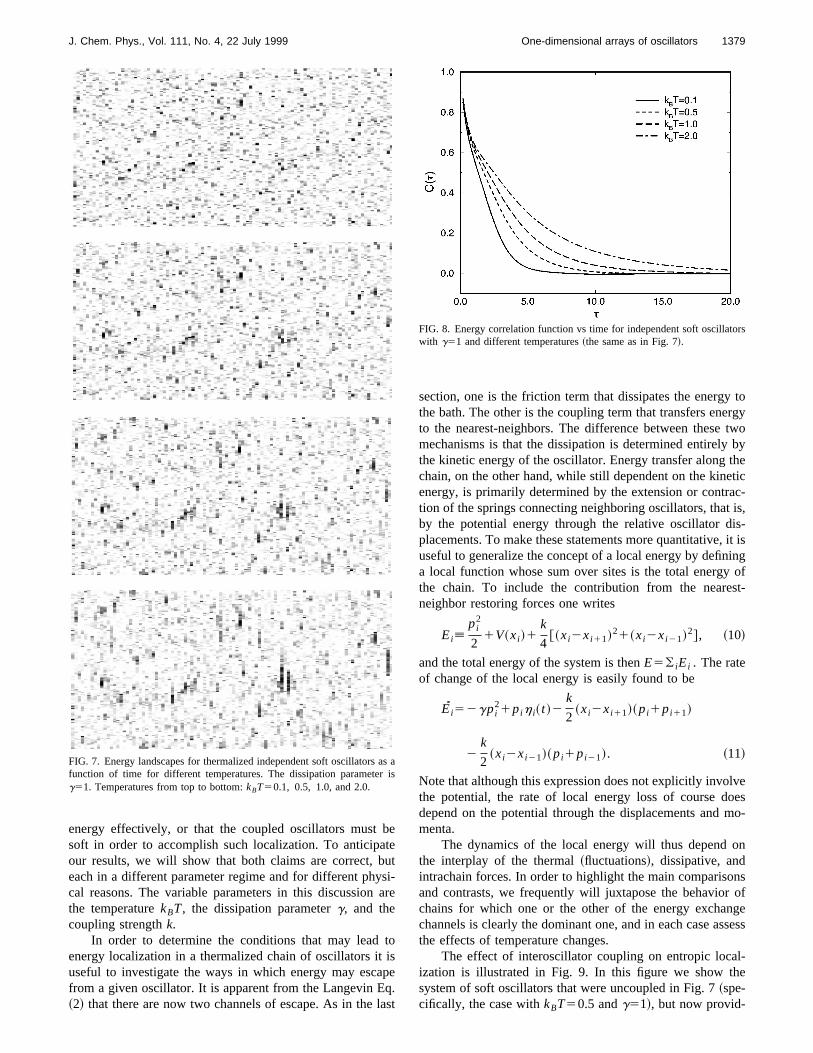
FIG. 7. Energy landscapes for thermalized independent soft oscillatorsfunction of time for different temperatures. The dissipation parameteg51. Temperatures from top to bottom:kBT50.1, 0.5, 1.0, and 2.0.
eeti-re
e.st
section, one is the friction term that dissipates the energthe bath. The other is the coupling term that transfers eneto the nearest-neighbors. The difference between thesemechanisms is that the dissipation is determined entirelythe kinetic energy of the oscillator. Energy transfer alongchain, on the other hand, while still dependent on the kineenergy, is primarily determined by the extension or contrtion of the springs connecting neighboring oscillators, thatby the potential energy through the relative oscillator dplacements. To make these statements more quantitativeuseful to generalize the concept of a local energy by defina local function whose sum over sites is the total energythe chain. To include the contribution from the neareneighbor restoring forces one writes
Ei[pi
2
21V~xi !1
k
4@~xi2xi 11!21~xi2xi 21!2#, ~10!
and the total energy of the system is thenE5( iEi . The rateof change of the local energy is easily found to be
Ei52gpi21pih i~ t !2
k
2~xi2xi 11!~pi1pi 11!
2k
2~xi2xi 21!~pi1pi 21!. ~11!
Note that although this expression does not explicitly invothe potential, the rate of local energy loss of course ddepend on the potential through the displacements andmenta.
The dynamics of the local energy will thus dependthe interplay of the thermal~fluctuations!, dissipative, andintrachain forces. In order to highlight the main comparisoand contrasts, we frequently will juxtapose the behaviorchains for which one or the other of the energy exchanchannels is clearly the dominant one, and in each case asthe effects of temperature changes.
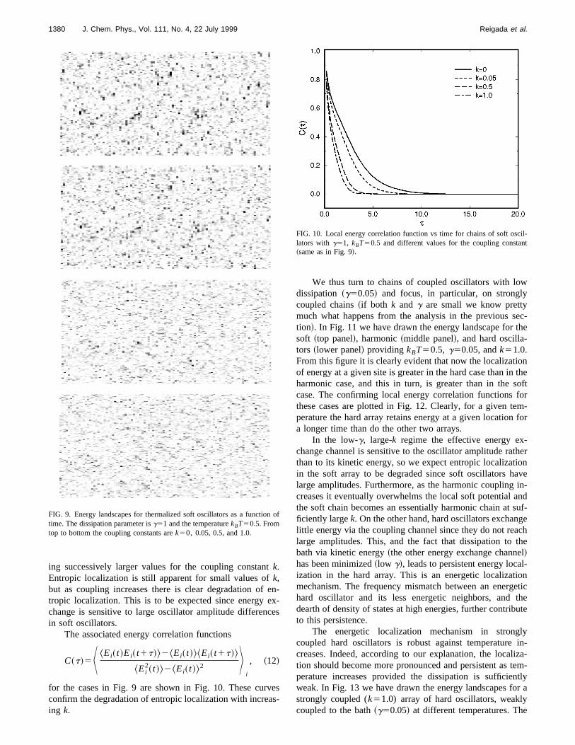
The effect of interoscillator coupling on entropic locaization is illustrated in Fig. 9. In this figure we show thsystem of soft oscillators that were uncoupled in Fig. 7~spe-cifically, the case withkBT50.5 andg51!, but now provid-
s ais
FIG. 8. Energy correlation function vs time for independent soft oscillatwith g51 and different temperatures~the same as in Fig. 7!.
t
eexce
ves
wy
ec-the
nthe
softform-for
-therionavein-
andsuf-gech
theell-onetictheute
lyin-
liza-tem-ntlyor aye
n
il-nt
1380 J. Chem. Phys., Vol. 111, No. 4, 22 July 1999 Reigada et al.
ing successively larger values for the coupling constank.Entropic localization is still apparent for small values ofk,but as coupling increases there is clear degradation oftropic localization. This is to be expected since energychange is sensitive to large oscillator amplitude differenin soft oscillators.
The associated energy correlation functions
C~t!5K ^Ei~ t !Ei~ t1t!&2^Ei~ t !&^Ei~ t1t!&
^Ei2~ t !&2^Ei~ t !&2 L
i
, ~12!
for the cases in Fig. 9 are shown in Fig. 10. These curconfirm the degradation of entropic localization with increaing k.
FIG. 9. Energy landscapes for thermalized soft oscillators as a functiotime. The dissipation parameter isg51 and the temperaturekBT50.5. Fromtop to bottom the coupling constants arek50, 0.05, 0.5, and 1.0.
n--s
s-
We thus turn to chains of coupled oscillators with lodissipation ~g50.05! and focus, in particular, on stronglcoupled chains~if both k and g are small we know prettymuch what happens from the analysis in the previous stion!. In Fig. 11 we have drawn the energy landscape forsoft ~top panel!, harmonic~middle panel!, and hard oscilla-tors ~lower panel! providing kBT50.5, g50.05, andk51.0.From this figure it is clearly evident that now the localizatioof energy at a given site is greater in the hard case than inharmonic case, and this in turn, is greater than in thecase. The confirming local energy correlation functionsthese cases are plotted in Fig. 12. Clearly, for a given teperature the hard array retains energy at a given locationa longer time than do the other two arrays.
In the low-g, large-k regime the effective energy exchange channel is sensitive to the oscillator amplitude rathan to its kinetic energy, so we expect entropic localizatin the soft array to be degraded since soft oscillators hlarge amplitudes. Furthermore, as the harmonic couplingcreases it eventually overwhelms the local soft potentialthe soft chain becomes an essentially harmonic chain atficiently largek. On the other hand, hard oscillators exchanlittle energy via the coupling channel since they do not realarge amplitudes. This, and the fact that dissipation tobath via kinetic energy~the other energy exchange chann!has been minimized~low g!, leads to persistent energy locaization in the hard array. This is an energetic localizatimechanism. The frequency mismatch between an energhard oscillator and its less energetic neighbors, anddearth of density of states at high energies, further contribto this persistence.
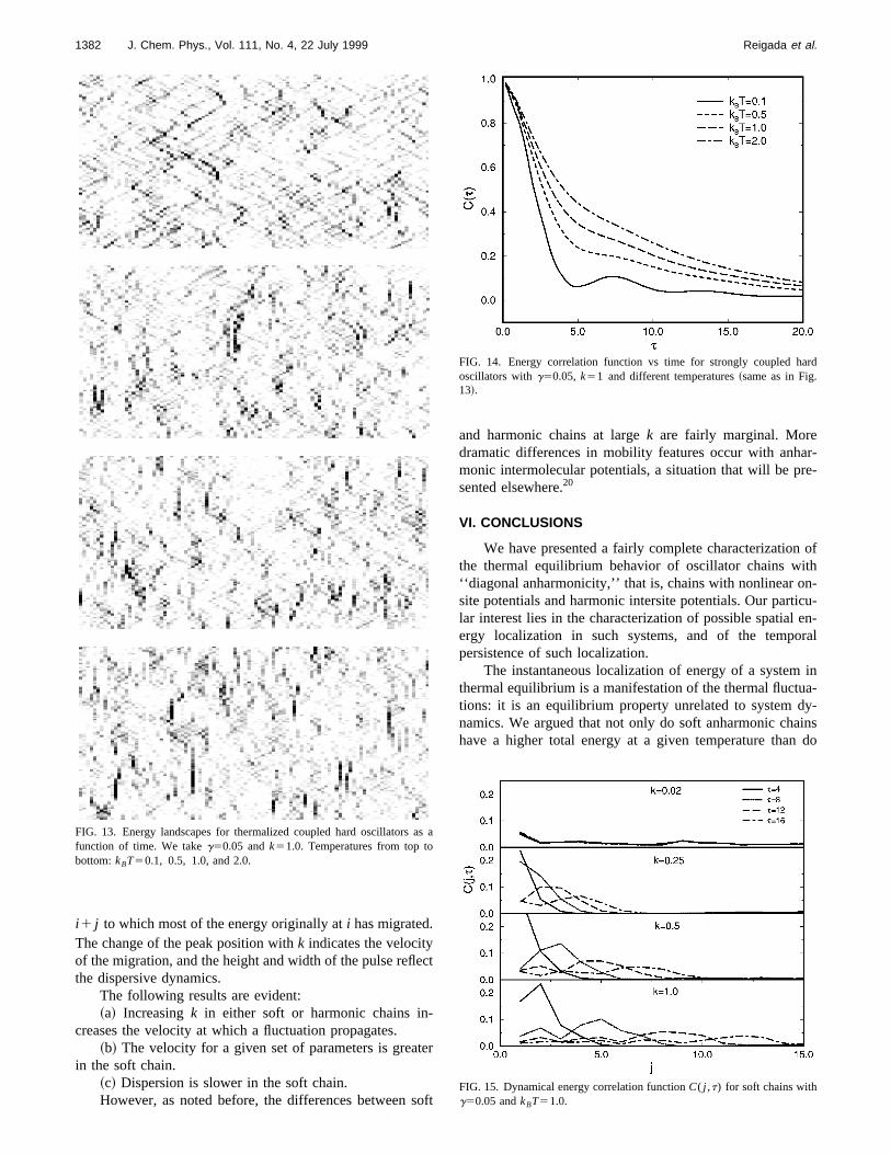
The energetic localization mechanism in strongcoupled hard oscillators is robust against temperaturecreases. Indeed, according to our explanation, the location should become more pronounced and persistent asperature increases provided the dissipation is sufficieweak. In Fig. 13 we have drawn the energy landscapes fstrongly coupled (k51.0) array of hard oscillators, weaklcoupled to the bath~g50.05! at different temperatures. Th
of
FIG. 10. Local energy correlation function vs time for chains of soft osclators with g51, kBT50.5 and different values for the coupling consta~same as in Fig. 9!.

rre14n-gltivinon-anein
heano
stuily
lec
do
hatar-
ore
ver,inceelyt the
ter-oftfteriseinnicpic
.gg.
cal
nantte
ith:
as
;
1381J. Chem. Phys., Vol. 111, No. 4, 22 July 1999 One-dimensional arrays of oscillators
figure qualitatively confirms these expectations. The cosponding energy correlation functions are plotted in Fig.C(t) for the hard chain does decay more slowly with icreasing temperature. Thus, localization in this stroncoupled system of hard oscillators becomes more effecwith increasing temperature and is not entirely fragile agadissipative forces. On the other hand, the soft and harmcorrelation functions~not shown here! are essentially independent of temperature. Note that the trend in Figs. 1214 is ‘‘opposite’’ to that of the uncoupled oscillators in thright hand panel of Fig. 4. In the strongly coupled chaharmonic and soft oscillators in fact lose their energy ratquickly on the time scale of one oscillation period ofisolated oscillator, but the hard oscillators retain energy crelations for longer than a period, indeed for many periodthe highest temperatures shown. With increasing temperathe hard oscillators retain energy more effectively even whthe average oscillation period decreases. In fact, the decathe correlation functions appears to involve two time scaone of the order of an oscillation period and another mulonger one that grows with temperature.
The temporal irregularities~oscillations! visible in Figs.
FIG. 11. Energy landscapes for thermalized strongly coupled oscillatorsfunction of time. The dissipation parameter isg50.05, the temperaturekBT50.5, and the coupling constantk51.0. Top panel: soft oscillatorsmiddle panel: harmonic oscillators; lower panel: hard oscillators.
-:
ye
stic
d
r
r-atreeof
s,h
12 and 14 are reproducibly there at all temperatures; wenot know their source.
V. MOBILITY OF LOCALIZED ENERGYFLUCTUATIONS
The upper two energy landscapes in Fig. 11 show wmight appear as fairly dispersionless energy transport. Nrow high-energy pulses move visibly along the chain befdisappearing, while others appear~via thermal fluctuations!to repeat the process elsewhere along the chain. Howethis cannot be claimed to represent nonlinear behavior sthe middle panel in Fig. 11 in fact represents a completharmonic system! This serves as a cautionary note abouoverinterpretation of such results.
We noted earlier that with increasingk the soft chaineventually becomes essentially harmonic because the inmolecular harmonic interactions overwhelm the local spotential~the only way to prevent this is by considering sointeroscillator interactions, which we defer to anothpaper!.20 The upper panel in Fig. 11 exhibits mostly thessentially harmonic behavior—it is quite similar to thmiddle panel—but not entirely so. The soft oscillator chaclearly shows higher-energy regions than the harmo~darker patches, a not fully degraded remnant of entrolocalization! that move more rapidly~steeper streaks! overlonger distances~longer streaks! than in the harmonic chainTherefore, the soft anharmonicity is clearly still playinsome role, albeit a diminishing one with increasing couplinTo provide some quantification, we introduce the dynamienergy correlation function
C~ j ,t!5K ^Ei~ t !Ei 1 j~ t1t!&2^Ei~ t !&^Ei 1 j~ t1t!&
^Ei2~ t !&2^Ei~ t !&2 L
i
.
~13!
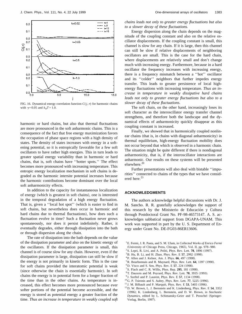
This correlation function plotted as a function ofj for varioustime differencest is shown in Fig. 15 for a soft chain and iFig. 16 for a harmonic chain. For a given coupling constk and delay timet, the correlation function peaks at the si
FIG. 12. Energy correlation function vs time for coupled oscillators wg50.05,kBT50.5, andk51.0. Solid line: harmonic potential. Dotted linesoft anharmonic potential. Dashed line: hard anharmonic potential.
a
ec
-
te
so
ar-e-
ofth-
cu-en-ral
ina-y-insdo
as
rd
1382 J. Chem. Phys., Vol. 111, No. 4, 22 July 1999 Reigada et al.
i 1 j to which most of the energy originally ati has migrated.The change of the peak position withk indicates the velocityof the migration, and the height and width of the pulse reflthe dispersive dynamics.
The following results are evident:~a! Increasingk in either soft or harmonic chains in
creases the velocity at which a fluctuation propagates.~b! The velocity for a given set of parameters is grea
in the soft chain.~c! Dispersion is slower in the soft chain.However, as noted before, the differences between
FIG. 13. Energy landscapes for thermalized coupled hard oscillatorsfunction of time. We takeg50.05 andk51.0. Temperatures from top tobottom:kBT50.1, 0.5, 1.0, and 2.0.
t
r
ft
and harmonic chains at largek are fairly marginal. Moredramatic differences in mobility features occur with anhmonic intermolecular potentials, a situation that will be prsented elsewhere.20
VI. CONCLUSIONS
We have presented a fairly complete characterizationthe thermal equilibrium behavior of oscillator chains wi‘‘diagonal anharmonicity,’’ that is, chains with nonlinear onsite potentials and harmonic intersite potentials. Our partilar interest lies in the characterization of possible spatialergy localization in such systems, and of the tempopersistence of such localization.
The instantaneous localization of energy of a systemthermal equilibrium is a manifestation of the thermal fluctutions: it is an equilibrium property unrelated to system dnamics. We argued that not only do soft anharmonic chahave a higher total energy at a given temperature than
a
FIG. 14. Energy correlation function vs time for strongly coupled haoscillators withg50.05, k51 and different temperatures~same as in Fig.13!.
FIG. 15. Dynamical energy correlation functionC( j ,t) for soft chains withg50.05 andkBT51.0.
onisoysof
src
Thdeac
ion
on
a
w,a
luyhith
seak
oinettho
lso
ag-os-hisel
ngin,
ngeardgy,orgygh-
insa
itsneldy-
his
n-
sain.alrented
u-id-
. J.of
ac-isn-
1383J. Chem. Phys., Vol. 111, No. 4, 22 July 1999 One-dimensional arrays of oscillators
harmonic or hard chains, but also that thermal fluctuatiare more pronounced in the soft anharmonic chains. Thisconsequence of the fact that free energy maximization favthe occupation of phase space regions with a high densitstates. The density of states increases with energy in aening potential, so it is entropically favorable for a few sooscillators to have rather high energies. This in turn leadgreater spatial energy variability than in harmonic or hachains, that is, soft chains have ‘‘hotter spots.’’ The effebecomes more pronounced with increasing temperature.entropic energy localization mechanism in soft chains isgraded as the harmonic intersite potential increases becthe harmonic contributions become dominant over the losoft anharmonicity effects.
In addition to the capacity for instantaneous localizatof energy~which is greatest in soft chains!, one is interestedin the temporal degradation of a high energy fluctuatiThat is, given a ‘‘local hot spot’’~which is easier to find insoft chains, but nevertheless does occur in harmonichard chains due to thermal fluctuations!, how does such afluctuation evolve in time? Such a fluctuation never grospontaneously, nor does it persist indefinitely. Rathereventually degrades, either through dissipation into the bor through dispersion along the chain.
The rate of dissipation into the bath depends on the vaof the dissipation parameter and also on the kinetic energthe oscillators. If the dissipation parameter is small, tchannel is of course slow for any chain. However, even ifdissipation parameter is large, dissipation can still be slowthe energy is not primarily in kinetic form. This is the cafor soft chains provided the interatomic potential is we~since otherwise the chain is essentially harmonic!. In softchains the energy is in potential form for a longer fractionthe time than in the other chains. As temperature iscreased, this effect becomes more pronounced becausesofter portions of the potential become accessible, andenergy is stored as potential energy a greater fraction oftime.Thus an increase in temperature in weakly coupled s
FIG. 16. Dynamical energy correlation functionC( j ,t) for harmonic chainswith g50.05 andkBT51.0.
sa
rsofft-
ttodtis-
useal
.
nd
sitth
eofseif
f-ver
hee
ft
chains leads not only to greater energy fluctuations but ato a slower decay of these fluctuations.
Energy dispersion along the chain depends on the mnitude of the coupling constant and also on the relativecillator displacements. If the coupling constant is small, tchannel is slow for any chain. If it is large, then this channcan still be slow if relative displacements of neighborioscillators are small. This is the case for the hard chawhere displacements are relatively small and don’t chamuch with increasing energy. Furthermore, because in a hoscillator the frequency increases with increasing enerthere is a frequency mismatch between a ‘‘hot’’ oscillatand its ‘‘colder’’ neighbors that further impedes enertransfer. This leads to greater persistence of local hienergy fluctuations with increasing temperature.Thus an in-crease in temperature in weakly dissipative hard chaleads not only to greater energy fluctuations but also toslower decay of these fluctuations.
The soft chain, on the other hand, increasingly losessoft character as the interoscillator energy transfer chanstrengthens, and therefore both the landscape and thenamical effects of anharmonicity quickly disappear as tcoupling constant is increased.
Finally, we showed that in harmonically coupled nonliear chains~that is, in chains with diagonal anharmonicity! inthermal equilibrium, high-energy fluctuation mobility doenot occur beyond that which is observed in a harmonic chThe situation might be quite different if there is nondiagonanharmonicity, that is, if the interoscillator interactions aanharmonic. Our results on these systems will be preseelsewhere.20
Further presentations will also deal with bistable ‘‘imprities’’ connected to chains of the types that we have consered here.23
ACKNOWLEDGMENTS
The authors acknowledge helpful discussions with DrM. Sancho. R. R. gratefully acknowledges the supportthis research by the Ministerio de Educacio´n y Culturathrough Postdoctoral Grant No. PF-98-46573147. A. S.knowledges sabbatical support from DGAPA-UNAM. Thwork was supported in part by the U. S. Department of Eergy under Grant No. DE-FG03-86ER13606.
1E. Fermi, J. R. Pasta, and S. M. Ulam, inCollected Works of Enrico Fermi~University of Chicago Press, Chicago, 1965!, Vol. II, pp. 978–980.
2S. Lepri, R. Livi, and A. Politi, Phys. Rev. Lett.78, 1896~1997!.3B. Hu, B. Li, and H. Zhao, Phys. Rev. E57, 2992~1998!.4P. Allen and J. Kelner, Am. J. Phys.66, 497 ~1998!.5R. Bourbonnais and R. Maynard, Phys. Rev. Lett.64, 1397~1990!.6D. Visco and S. Sen, Phys. Rev. E57, 224 ~1998!.7S. Flach and C. R. Willis, Phys. Rep.295, 181 ~1998!.8T. Dauxois and M. Peyrard, Phys. Rev. Lett.70, 3935~1993!.9J. Szeftel and P. Laurent, Phys. Rev. E57, 1134~1998!.
10G. P. Tsironis and S. Aubry, Phys. Rev. Lett.77, 5225~1996!.11J. M. Bilbault and P. Marquie´, Phys. Rev. E53, 5403~1996!.12D. W. Brown, L. J. Bernstein and K. Lindenberg, Phys. Rev. E54, 3352
~1996!; K. Lindenberg, L. Bernstein, and D. W. Brown, inStochasticDynamics, edited by L. Schimansky-Geier and T. Peoschel~Springer-Verlag, Berlin, 1997!.
L
II
:
sics,
1384 J. Chem. Phys., Vol. 111, No. 4, 22 July 1999 Reigada et al.
13A. J. Sievers and S. Takeno, Phys. Rev. Lett.61, 970~1988!; K. Hori andS. Takeno, J. Phys. Soc. Jpn.61, 2186~1992!; ibid. 61, 4263~!; S. Tak-eno, ibid. 61, 2821~1992!.
14V. E. Zakharov, Sov. Phys. JETP35, 908 ~1972!.15J. F. Lindsner, S. Chandramouli, A. R. Bulsara, M. Locher, and W.
Ditto, Phys. Rev. Lett.81, 5048~1998!.16K. Lindenberg, D. W. Brown, and J. M. Sancho, Proceedings of the V
Spanish Meeting on Statistical Physics FISES ’97, Anales de Fı´sica,Monografıas RSEF4, 3 ~1998!.
17T. Pullerits and V. Sundstrom, Acc. Chem. Res.29, 381 ~1996!; X. Huand K. Schulten, Phys. Today50, 28 ~1997!.
18P. L. Christiansen and A. C. Scott, editors,Davydov’s Soliton Revisited
.
I
Self-Trapping of Vibrational Energy in Protein, NATO ASI Ser., Ser. B243, ~Plenum Press, New York, 1990!.
19C. Van den Broeck, J. M. Parrondo, and R. Toral, Phys. Rev. Lett.73,3395 ~1994!.
20A. Sarmiento, R. Reigada, A. H. Romero, and K. Lindenberg~unpub-lished!.
21T. C. Gard,Introduction to Stochastic Differential Equations~Marcel De-kker, New York, 1987!.
22R. Toral, in Computational Field Theory and Pattern Formation, 3rdGranada Lectures in Computational Physics, Lecture Notes in PhyVol. 448 ~Springer-Verlag, Berlin, 1995!.
23R. Reigada, A. Sarmiento, J. M. Sancho, and K. Lindenberg~unpub-lished!.


![Travelling waves in chains of pulse-coupled integrate-and …bresslof/publications/99-2.pdfrhythms [1,2], chemical oscillators [3], Josephson junction arrays [4,5] and laser arrays](https://img.pdfslide.net/doc/110x75/60f69f2c60224e083c5e9cc1/travelling-waves-in-chains-of-pulse-coupled-integrate-and-bresslofpublications99-2pdf.jpg)