One-Dimensional Graph Drawing:Part I — Drawing Graphs by Axis Separation

Yehuda Koren and David Harel

Dept. of Computer Science and Applied MathematicsThe Weizmann Institute of Science, Rehovot, Israel

{yehuda,dharel}@wisdom.weizmann.ac.il

Abstract. In this paper we discuss a useful family of graph drawing algorithms,characterized by their ability to draw graphs in one dimension. The most importantapplication of this family seems to be achieving graph drawing by axis separation,where each axis of the drawing addresses different aspects of aesthetics. We de-fine the special requirements from such algorithms and show how several graphdrawing algorithms can be generalized to handle this task.

1 Introduction

A graph G(V,E) is an abstract structure that is used to model a relation E over a set V ofentities. Graph drawing is a standard means for the visualization of relational informa-tion, and its ultimate usefulness depends on the readability of the resulting layout; thatis, the drawing algorithm’s capability of conveying the meaning of the diagram quicklyand clearly. Consequently, many approaches to graph drawing have been developed [6,15]. We concentrate on the problem of drawing graphs so as to convey pictorially theproximity relations between the nodes. The most popular approaches to this appear to beforce-directed algorithms. These define a cost function (or a force model), whose min-imization determines the optimal drawing. Graph drawing research traditionally dealswith drawing graphs in two or three dimensions. In this paper, we identify and discuss anew family of graph drawing algorithms whose goal is to draw the graph in one dimen-sion. This family has some interesting applications, to which we now turn.

Axis separation The most common use of 1-D drawing algorithms is graph drawingby axis separation. Here, we would like to build a multidimensional layout axis-by-axis,so that we each axis can be computed using a different algorithm, perhaps accounting fordifferent aesthetical considerations. This facilitates an appealing “divide-and-conquer”approach to graph drawing. A well known example of this is the problem of drawingdirected graphs, where the y-coordinates are commonly used to reflect the hierarchy,while the separately computed x-coordinates take care of additional characteristics ofthe graph, such as preserving proximity.

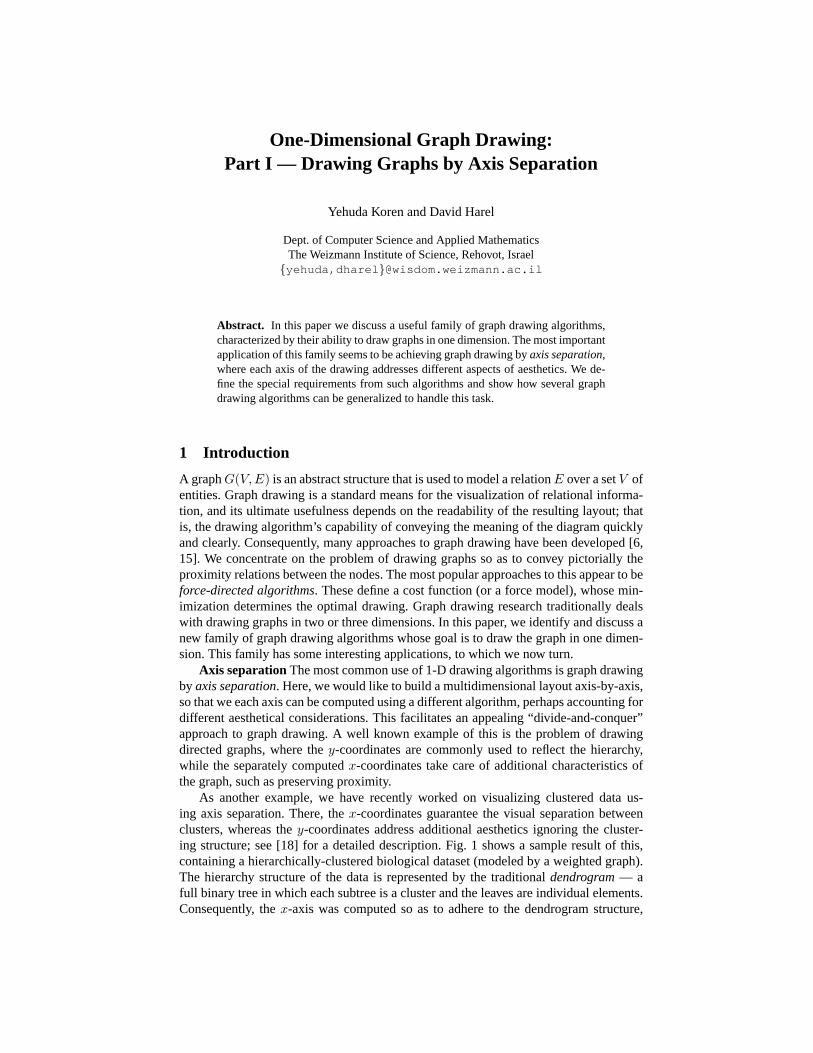
As another example, we have recently worked on visualizing clustered data us-ing axis separation. There, the x-coordinates guarantee the visual separation betweenclusters, whereas the y-coordinates address additional aesthetics ignoring the cluster-ing structure; see [18] for a detailed description. Fig. 1 shows a sample result of this,containing a hierarchically-clustered biological dataset (modeled by a weighted graph).The hierarchy structure of the data is represented by the traditional dendrogram — afull binary tree in which each subtree is a cluster and the leaves are individual elements.Consequently, the x-axis was computed so as to adhere to the dendrogram structure,

while maximizing the expression of similarities between the nodes. This was done byreordering the dendrogram and adjusting the gaps between consecutive leaves. The y-axis, which should not consider the hierarchy structure at all, was computed by a 1-Dgraph drawing algorithm (using the classical-MDS method, as described in Subsection3.3).

Fig. 1. (taken from [18]) Using axis-separation to draw hierarchically clustered fibroblast geneexpression data. We convey both the similarities between the nodes and their clustering decom-position, using an ordered dendrogram coupled with a 2-D layout that adheres to its structure. Wehave colored six salient clusters that are clearly visible.

Sometimes a single dataset can be modeled by different graphs. Consequently, itmight be instructive to draw the data by assigning each of the axes to a different graph,and then simultaneously examine and compare the characteristics of the two models.For example, proximity relationships between web pages can be modeled either by con-necting pages that have a similar content, or by relying on their link structure. We candraw the web pages as points in the plane according to these two models by using axisseparation, thus making it possible to see at a glance which elements are related by eachof them.

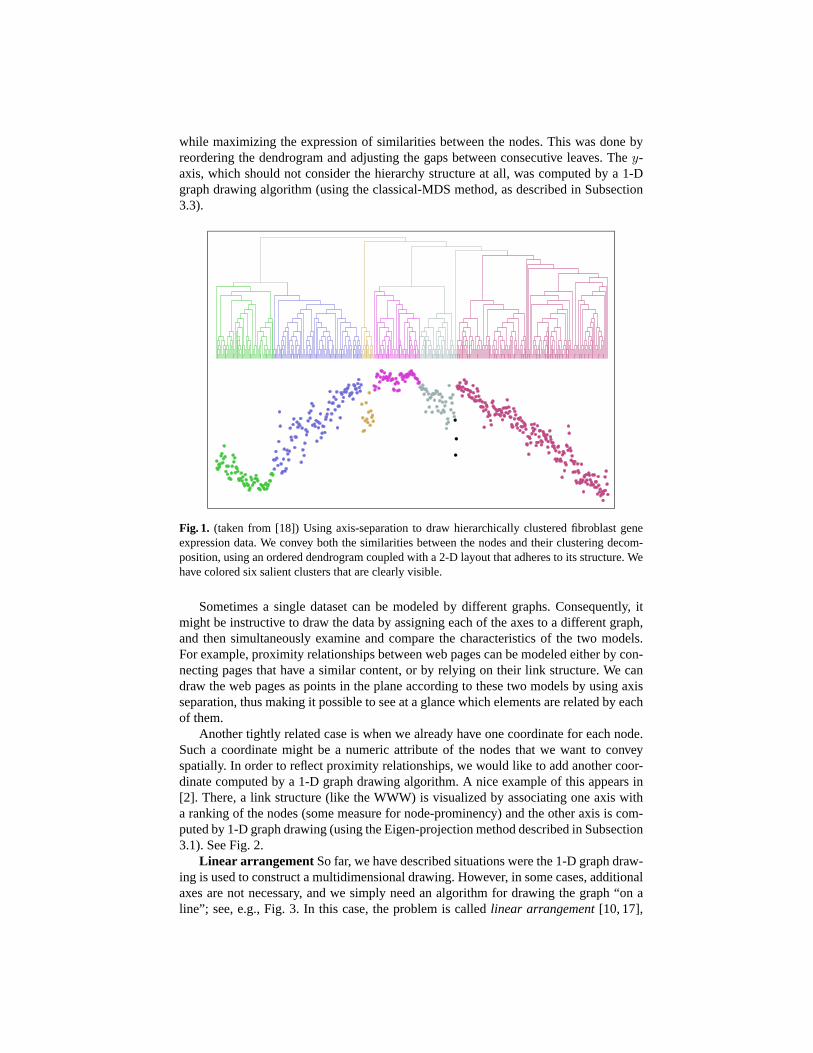
Another tightly related case is when we already have one coordinate for each node.Such a coordinate might be a numeric attribute of the nodes that we want to conveyspatially. In order to reflect proximity relationships, we would like to add another coor-dinate computed by a 1-D graph drawing algorithm. A nice example of this appears in[2]. There, a link structure (like the WWW) is visualized by associating one axis witha ranking of the nodes (some measure for node-prominency) and the other axis is com-puted by 1-D graph drawing (using the Eigen-projection method described in Subsection3.1). See Fig. 2.

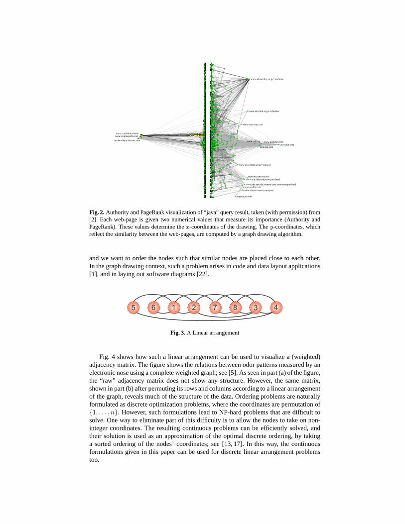
Linear arrangement So far, we have described situations were the 1-D graph draw-ing is used to construct a multidimensional drawing. However, in some cases, additionalaxes are not necessary, and we simply need an algorithm for drawing the graph “on aline”; see, e.g., Fig. 3. In this case, the problem is called linear arrangement [10, 17],

javaboutique.internet.com

www.scriptsearch.com Stars.com/Multimedia/

www.phy.syr.edu/courses/java-suite/crosspro.html

physics.syr.edu

www.gamelan.com

java.sun.com

www.china-contact.com/java/www.javafile.com

www.stat.duke.edu/sites/java.html

www.nep.chubu.ac.jp/~nepjava/

tacocity.com.tw/java/

www.w3.org

www.auscomp.com

home.interlink.or.jp/~ichisaka/

www.sun.com

www.sikasenbey.or.jp/~ueshima/

Fig. 2. Authority and PageRank visualization of “java” query result, taken (with permission) from[2]. Each web-page is given two numerical values that measure its importance (Authority andPageRank). These values determine the x-coordinates of the drawing. The y-coordinates, whichreflect the similarity between the web-pages, are computed by a graph drawing algorithm.

and we want to order the nodes such that similar nodes are placed close to each other.In the graph drawing context, such a problem arises in code and data layout applications[1], and in laying out software diagrams [22].

� ��� � � � �

Fig. 3. A Linear arrangement

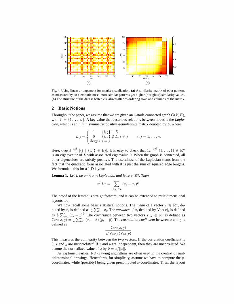
Fig. 4 shows how such a linear arrangement can be used to visualize a (weighted)adjacency matrix. The figure shows the relations between odor patterns measured by anelectronic nose using a complete weighted graph; see [5]. As seen in part (a) of the figure,the “raw” adjacency matrix does not show any structure. However, the same matrix,shown in part (b) after permuting its rows and columns according to a linear arrangementof the graph, reveals much of the structure of the data. Ordering problems are naturallyformulated as discrete optimization problems, where the coordinates are permutation of{1, . . . , n}. However, such formulations lead to NP-hard problems that are difficult tosolve. One way to eliminate part of this difficulty is to allow the nodes to take on non-integer coordinates. The resulting continuous problems can be efficiently solved, andtheir solution is used as an approximation of the optimal discrete ordering, by takinga sorted ordering of the nodes’ coordinates; see [13, 17]. In this way, the continuousformulations given in this paper can be used for discrete linear arrangement problemstoo.

(a) (b)

Fig. 4. Using linear arrangement for matrix visualization. (a) A similarity matrix of odor patternsas measured by an electronic nose; more similar patterns get higher (=brighter) similarity values.(b) The structure of the data is better visualized after re-ordering rows and columns of the matrix.

2 Basic NotionsThroughout the paper, we assume that we are given an n-node connected graph G(V,E),with V = {1, . . . , n}. A key value that describes relations between nodes is the Lapla-cian, which is an n × n symmetric positive-semidefinite matrix denoted by L, where

Lij =

−1 {i, j} ∈ E0 {i, j} /∈ E, i �= j

deg(i) i = ji, j = 1, . . . , n.

Here, deg(i) def= |{j | {i, j} ∈ E}|. It is easy to check that 1ndef= (1, . . . , 1) ∈ R

n

is an eigenvector of L with associated eigenvalue 0. When the graph is connected, allother eigenvalues are strictly positive. The usefulness of the Laplacian stems from thefact that the quadratic form associated with it is just the sum of squared edge lengths.We formulate this for a 1-D layout:

Lemma 1. Let L be an n × n Laplacian, and let x ∈ Rn. Then

xT Lx =∑

{i,j}∈E

(xi − xj)2.

The proof of the lemma is straightforward, and it can be extended to multidimensionallayouts too.

We now recall some basic statistical notions. The mean of a vector x ∈ Rn, de-

noted by x, is defined as 1n

∑ni=1 xi. The variance of x, denoted by Var(x), is defined

as 1n

∑ni=1 (xi − x)2. The covariance between two vectors x, y ∈ R

n is defined asCov(x, y) = 1

n

∑ni=1 (xi − x) (yi − y). The correlation coefficient between x and y is

defined asCov(x, y)√

Var(x)Var(y)

This measures the colinearity between the two vectors. If the correlation coefficient is0, x and y are uncorrelated. If x and y are independent, then they are uncorrelated. Wedenote the normalized value of x by x = x/‖x‖.

As explained earlier, 1-D drawing algorithms are often used in the context of mul-tidimensional drawings. Henceforth, for simplicity, assume we have to compute the y-coordinates, while (possibly) being given precomputed x-coordinates. Thus, the layout

is characterized by two vectors x, y ∈ Rn, with the x-coordinates being x1, . . . , xn,

and the y-coordinates y1, . . . , yn. Other cases, where we have more than one precom-puted axis or where we want to produce several dimensions, can be addressed by smallchanges in our techniques. Moreover, for convenience, we assume, without loss of gen-erality, that the x- and y-coordinates are centered, so their means are 0. In symbols,∑n

i=1 xi =∑n

i=1 yi = 0. This can be achieved by a simple translation.

3 Algorithms for One-Dimensional Graph Drawing

In principle, we could have used a classical force-directed algorithm for computing the1-D layout. However, when trying to modify the customary two-dimensional optimiza-tion algorithm for use in our one-dimensional case, convergence was rarely achieved.Traditionally, node-by-node optimization is performed, by moving each node to a pointthat decreases the cost function. Common methods for this are Gradient-Descent andNewton-Raphson. However, these methods tend to get stuck in bad local minima whenused for 1-D drawing [4, 23]. Interestingly, 2-D drawing is much easier for such meth-ods. Probably, the reason is that there is less space for maneuver in one dimension whenseeking a nice layout, which prevents convergence to an optimum. Furthermore, in sev-eral works even a 3-D layout is used to avoid local minima, see, e.g., [3, 8, 23].

Another possible approach could be to use algorithms for computing (approximated)minimum linear arrangements (MinLA). These set the coordinates to be a permutation of{1, . . . , n} in a way that minimizes the sum of edge lengths. Although the limitation thatthe coordinates are distinct integers may seem unnatural in the graph drawing context,we have found that MinLA has some merits when drawing digraphs by axis separation;see [4]. However, a major disadvantage of MinLA is that it cannot consider precomputedcoordinates. Note that a careless computation that ignores such precomputed coordinatescan be very problematic. Such a computation might yield y-coordinates that are verysimilar to the x-coordinates, resulting in a drawing whose intrinsic dimensionality wouldreally be 1, meaning that one axis would be wasted.

In the rest of this section, we describe four different methods that appear to be per-fect for our task. A common characteristic of these methods, which makes them suitablefor 1-D optimization, is that they compute the layout axis-by-axis, instead of the node-by-node optimization mechanism of force-directed methods. Furthermore, when thesemethods are used to produce a multidimensional layout, the different axes are uncor-related. This suggests a very effective way to generalize the methods so that they candeal with the precomputed coordinates: we simply require no correlation between thex-coordinates and the y-coordinates, so that the latter ones will provide us with as muchnew information as possible. Technically, since we have assumed x and y to be centered,the no-correlation requirement can be formulated simply as yT ·x = 0, which states thatx and y are orthogonal.

We now survey the methods and explain how they can be extended to handle thecase of predefined x-coordinates.

3.1 Eigen-projection

The Eigen-projection [11, 19] computes the layout of a graph using low eigenvectors ofthe related Laplacian. Some important advantages of this approach are its ability to com-pute optimal layouts (according to specific requirements) and a very short computationtime [16]. As we will see, this method is a natural choice for 1-D layouts, and has al-ready been used for such tasks in [13, 1, 2, 4]. In [19] we give several explanations for the

ability of the Eigen-projection to draw graphs nicely. Here, we provide a new derivation,which shows the tight relationship of this method to force-directed graph drawing.

We define the Eigen-projection 1-D layout y ∈ Rn, as the solution of:

miny

∑{i,j}∈E(yi − yj)2∑{i,j}/∈E(yi − yj)2

(1)

In (1), the numerator calls for shortening the edge lengths (the “attractive forces”),while the denominator calls for placing all nonadjacent pairs further apart (the “repul-sive forces”). This is a reasonable energy minimization approach that resembles force-directed algorithms.

Since we have∑

{i,j}∈E(yi − yj)2 +∑

{i,j}/∈E(yi − yj)2 =∑

i<j(yi − yj)2, anequivalent problem would be:

miny

∑{i,j}∈E(yi − yj)2∑

i<j(yi − yj)2(2)

It is easy to see that the energy to be minimized is invariant under translation of thedata. Thus, for convenience, we eliminate this degree of freedom, by requiring that y becentered; that is, yT 1n = 0. We can now simplify (2) by using the following lemma:

Lemma 2. Let y ∈ Rn such that yT 1n = 0, then:

∑i<j

(yi − yj)2 = n ·n∑

i=1

y2i (= n · yT y) .

Proof.

∑i<j

(yi − yj)2 =12

n∑i,j=1

(yi − yj)2 =12

2n

n∑i=1

y2i − 2

n∑i,j=1

yiyj

=

= n ·n∑

i=1

y2i −

n∑i=1

yi

n∑j=1

yj = n ·n∑

i=1

y2i

The last step stems from the fact that y is centered, so that∑n

j=1 yj = 0. ��

Therefore, we can replace∑

i<j(yi − yj)2 with yT y. Moreover, using Lemma 1, wecan write

∑{i,j}∈E(yi − yj)2 as the quadratic form yT Ly. Consequently, once again

we reformulate our minimization problem in the equivalent form:

miny

yT Ly

yT y

in the subspace: yT 1n = 0(3)

By substituting x = 0 in the following Proposition, we obtain that the optimal 1-Dlayout is the eigenvector of L with the smallest positive eigenvalue.

This way, the Eigen-projection method provides us with an efficient way to calculateoptimal 1-D layouts. We still have to show how the Eigen-projection can be extendedso as to deal with the uncorrelation requirement, that is a case where we already have a

coordinate vector x, and we require that y is orthogonal to x. Now, the optimal layoutwill be the solution of:

miny

yT Ly

yT y

in the subspace: yT 1n = 0, yT x = 0(4)

Fortunately, the optimal layout is still a solution of a related eigen-equation:

Proposition 1. The solution of (4) is the eigenvector of (I − xxT )L(I − xxT ) with thesmallest positive eigenvalue.

(Note that I − xxT is a symmetric n × n matrix. Henceforth, we will use it extensivelythanks to its property of being an orthogonalization operator: for any vector y ∈ R

n, theresult of orthogonalizing y against x is (I − xxT )y.)

Proof. Observe that we can assume, without loss of generality, that yT y = 1. This isbecause changing the scale still gives an optimal solution: Check that if for y0 satisfyingyT0 y0 = 1 we get yT

0 Ly0/yT0 y0 = λ, then we will also get yT Ly/yT y = λ for each

y = c · y0 (c �= 0). Thus, the new form of the optimization problem will be:

miny

yT Ly

given: yT y = 1

in the subspace: yT 1n = 0, yT x = 0

(5)

The matrix (I − xxT )L(I − xxT ) is symmetric, so it has n orthogonal eigenvectorsspanning R

n. We will use the convention λ1 ≤ λ2 ≤ . . . ≤ λn for the eigenvalues of(I − xxT )L(I − xxT ), and denote the corresponding real orthonormal eigenvectors byu1, u2, . . . , un. Clearly, (I − xxT )L(I − xxT ) ·x = 0. Utilizing the fact that xT 1n = 0and that 1n is the only zero eigenvector of L, we obtain λ1 = λ2 = 0, u1 = (1/‖1n‖) ·1n, u2 = x, and λ3 > 0.

We can now decompose every y ∈ Rn as a linear combination, where y =

∑ni=1 αiui.

Moreover, since the solution is constrained to be orthogonal to u1 and u2, we can restrictourselves to linear combinations of the form y =

∑ni=3 αiui.

Use the constraint yT y = 1 to obtain∑n

i=3 α2i = 1 (a generalization of the Pythagorean

law). Similarly, yT (I−xxT )L(I−xxT )y =∑n

i=3 α2i λi. Note that since yT x = xT y =

0, we get:

yT (I − xxT )L(I − xxT )y = yT Ly + yT xxT L(I − xxT )y + yT LxxT y = yT Ly .

So the target value is

yT Ly = yT (I − xxT )L(I − xxT )y =n∑

i=3

α2i λi �

n∑i=3

α2i λ3 = λ3.

Thus, for any y that satisfies the constraints, we get yT Ly � λ3. Since uT3 Lu3 =

uT3 (I − xxT )L(I − xxT )u3 = λ3, we can deduce that the minimizer is u3, the lowest

positive eigenvector. ��

Interestingly, posing the problem as in (4) and solving it as in Proposition 1, con-stitutes a smooth generalization of the Eigen-projection method: when x is the lowestpositive eigenvector of L, then the solution y will be the second lowest positive eigen-vector of L. This coincides with the way the Eigen-projection computes 2-D layouts;see [19]. However, we allow the more general case of arbitrary x-coordinates.

As to computational complexity, the space requirement of the algorithm is O(|E|)when using a sparse representation of the Laplacian. The computation can be done usingiterative algorithms, such as the Power-Iteration or Lanczos; see [9]. The time com-plexity of a single iteration is O(|E|). When working with a sparse L, we can usea much faster multi-scale algorithm that can deal with millions of elements in rea-sonable time; see [16]. However, caution is needed, since an explicit calculation of(I − xxT )L(I − xxT ) would destroy the sparsity of L. To get around this, we uti-lize the fact that the iterative algorithms for computing eigenvectors use the matrix asan operator, i.e., they access it only via multiplication with a vector. This settles theissue, since carrying out the product (I − xxT )L(I − xxT ) · v is equivalent to orthog-onalizing v against x, multiplying the result with the sparse matrix L, and then againorthogonalizing the result against x.

3.2 Principal component analysis and high-dimensional embeddingPrincipal component analysis (PCA) computes a projection of multidimensional datathat optimally preserves its variance; see [7]. The fact that PCA uses the data coordinatesapparently renders it useless for graph drawing. However, in [12] we show that it ispossible to generate artificial k-dimensional coordinates of the nodes that preserve someof the graph structure, thus making it possible to use PCA. We call these coordinateshigh-dimensional embedding in [12], and denote them by an n × k coordinate matrixcalled X , so the k coordinates of node i constitute the i-th row of X . We assume eachof the columns of X is centered, something that can be achieved by translating the data.In order to compute a 1-D projection, PCA computes a unit vector d ∈ R

k, which is thedirection of the projection. The vector d is the top eigenvector of the covariance matrix1nX TX . The projection itself is Xd, and, as mentioned, it is the best 1-D projection interms of variance preservation.

When given x-coordinates, we will be interested only in the component of the projec-tion that is orthogonal to the x-coordinates. This component is exactly (I− xxT ) ·(Xd),and we want to maximize its variance. However,

(I − xxT ) · (Xd) = ((I − xxT ) · X )d,

so our problem is reduced to finding the most variance-preserving projection of thecoordinates (I − xxT ) · X . The optimal solution is obtained by performing PCA on(I − xxT ) · X , which is equivalent to orthogonalizing each of X columns against x andthen performing PCA on the resulting matrix.

Again, this is a smooth generalization of PCA that enables it to deal with predefinedx-coordinates. The reason is that if x was also computed by PCA, then one would ob-tain the regular 2-D PCA projection. One of the advantages of the PCA approach is itsexcellent time and space complexity; see [12].

3.3 Classical multidimensional scalingMultidimensional scaling (MDS) is a general term for techniques that generate coordi-nates of points from information about pairwise distances. Therefore, arguably, force-directed graph drawing can be considered to be MDS. Here we are interested in a tech-nique called classical-MDS (CMDS) [7], which produces (multidimensional) coordi-nates that preserve the given pairwise distances perfectly; i.e., the pairwise Euclidean

distances in the generated space are equal to the given distances. The graph drawingapplication of CMDS was suggested long ago, in [21]. The distance between nodes iand j is defined as dij , the graph-theoretical distance between the nodes. Therefore,CMDS can be used to find an Euclidean embedding of the graph that preserves thegraph-theoretical distance.

We now provide a short technical description of the method. Given points in Eu-clidean space, it is possible to construct a matrix X of centered coordinates if we knowthe pairwise distances among the points. The way to do this is to construct the n×n innerproduct matrix B = XX T , which can be computed using the cosine law, as follows

Bij = −12

d2

ij −1n

n∑k=1

d2ik − 1

n

n∑k=1

d2kj +

1n2

n∑k=1,l=1

d2lk

. (6)

Note that B is invariant under orthogonal transformations of X . That is, given someorthogonal matrix Q (i.e., QQT = I), we can replace X with XQ, without changing theinner-product matrix:

XQ(XQ)T = XQQTX = XX T = B

Therefore, B determines the coordinates up to orthogonal transformation. This is rea-sonable, since such a transformation does not alter pairwise distances. There is alwaysan orthogonal transformation that makes the axes orthogonal (i.e., the singular valuedecomposition), which allows us to restrict ourselves to a coordinate matrix with or-thogonal columns. Such a matrix can be obtained by factoring B using the eigenvaluedecomposition B = U∆UT (U is orthogonal and ∆ is diagonal), which enables defin-ing the coordinates of the points as X = U∆

12 . This way, the columns of X are centered

and are mutually orthogonal. In practice, we do not want all the coordinates but onlya low-dimensional projection of the points, and here only a 1-D embedding is needed.Thus, as in PCA, we seek the 1-D projection of X having the maximal variance. Sincethe columns of X are uncorrelated, we simply have to take the column with the maximalvariance, which is equivalent to the column of U with the highest corresponding eigen-value. Technically, we are interested in the top eigenvector u1 and the correspondingeigenvalue, λ1, of B. After computing this eigenpair, we can define the embedding ofthe data as

√λ1u1. Additional coordinates can be obtained using the subsequent eigen-

pairs.It appears that CMDS is closely related to PCA. In fact, CMDS is a way of per-

forming PCA without explicitly defining the coordinate matrix. Thus, if the pairwisedistances are Euclidean distances based on the coordinate matrix, the results of CMDSare identical to PCA. Consequently, in our case, when we want the embedding to beorthogonal to x, we can use the same technique we used in PCA.

Once again, we would like to perform PCA on (I− xxT )X , and of course we do nothave this matrix explicitly. However, it is possible to compute the inner-product matrix(I − xxT )XX T (I − xxT ), since this matrix is simply (I − xxT )B(I − xxT ). Usingthe same reasoning as above, the first principal component of (I − xxT )X can be foundby computing the top eigenpair of (I − xxT )B(I − xxT ).

However, there is one theoretical flaw in applying CMDS to graph-drawing. Com-puting a coordinate matrix X that preserves pairwise distances is not always possible,and will fail when the graph-theoretic metric is not Euclidean. Technically, there mightbe some negative eigenvalues to the matrix B, preventing the square-root operation from

being carried out. However, in practice this is not a serious problem, since we are notinterested in recovering the full multidimensional coordinates, but only the few leadingcoordinates.

When the given x-coordinates are also the result of CMDS, our method produces thesame y-coordinates as CMDS. Therefore, we have a smooth generalization of CMDSthat allows it to deal with predefined coordinates.

One note on complexity. When performing this CMDS, we have to store the matrixB, which requires O(n2) space complexity, much worse than in the Eigen-projection orPCA cases.

3.4 One-dimensional drawing of digraphsWhen edges are directed, we may want the layout to show the overall directionalityof the graph and its hierarchical structure. The previously described techniques, whichignore the direction of the edges, might thus not be suitable. An adequate method fordealing with 1-D layout of digraphs was described in [4]. There, we looked for a layoutthat minimizes the hierarchy energy:

∑i→j∈E

(yi − yj − 1)2 (7)

Define the balance vector, b ∈ Rn, such that:

bi = outdeg(i) − indeg(i)

where outdeg(i) and indeg(i) denote the number of outgoing and incoming edges ad-jacent to i, respectively.

We showed in [4] that up to a constant additive term, the hierarchy energy (7), canbe written in a compact form as:

yT Ly − 2yT b (8)

Consequently, the optimal 1-D layout would be the solution of Ly = b. This formulationis flexible enough to allow y to be uncorrelated with a given coordinate vector x. In thiscase, we want to minimize (8) in the subspace orthogonal to x. Equivalently, we can takeonly the component of y that is orthogonal to x, which is (I− xxT )y. This way, we seekthe minimizer of:

yT (I − xxT )L(I − xxT )y − 2yT (I − xxT )b, (9)

Hence, the optimal 1-D layout would be the solution of:

(I − xxT )L(I − xxT )y = (I − xxT )b

After finding the minimizer we orthogonalize it against x. It is easy to see that this doesnot affect the value of (9), so we remain with an optimal solution uncorrelated with x.

As a consequence, when we have a 1-D layout of a digraph, we can add an additionaluncorrelated dimension that shows the hierarchical structure of the graph. Moreover, wecan compute two coordinate vectors that provide two uncorrelated descriptions of thegraph’s directionality. This might be useful for digraphs whose hierarchical structure isexplained by several independent factors.

When L is sparse, we recommended in [4] that the equation be solved using theConjugate-Gradient method that accesses L only via matrix-vector multiplication. Inthis case, like in the Eigen-projection case, the product (I − xxT )L(I − xxT ) · v iscarried out by orthogonalizing v against x, multiplying the result with the sparse matrixL, and then again orthogonalizing the result against x.

4 Discussion

We have explored one-dimensional graph drawing algorithms and have studied their spe-cial features and applications. One important application of this family is graph drawingby axis-separation, where each axis is computed separately, so as to address specificaesthetical considerations. Since point-by-point local optimization in one dimension isa poor strategy, traditional force-directed algorithms are not suitable for the 1-D draw-ing task, while less traditional algorithms are. We generalized four such algorithms us-ing the unified paradigm of computing the layout axis-by-axis, while maintaining non-correlation with the precomputed coordinates.

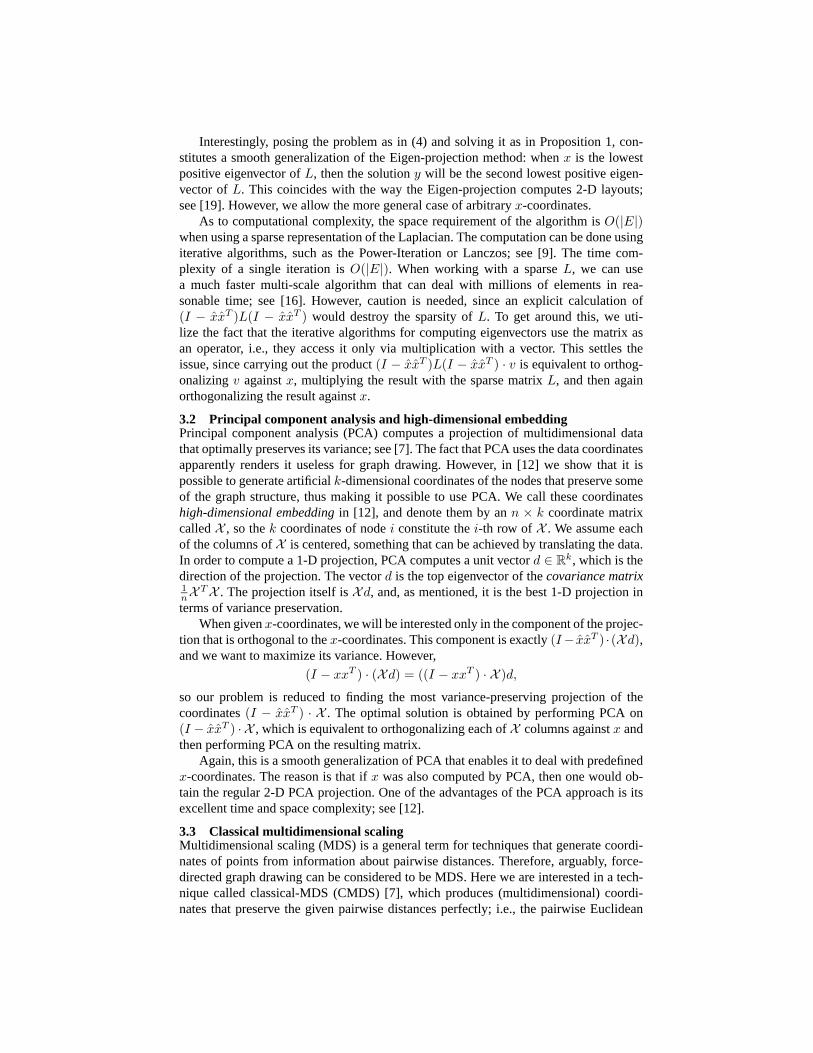
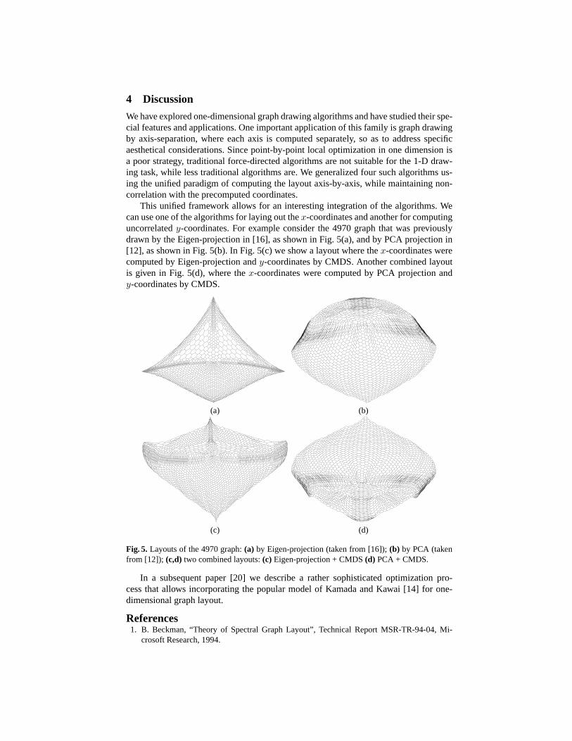
This unified framework allows for an interesting integration of the algorithms. Wecan use one of the algorithms for laying out the x-coordinates and another for computinguncorrelated y-coordinates. For example consider the 4970 graph that was previouslydrawn by the Eigen-projection in [16], as shown in Fig. 5(a), and by PCA projection in[12], as shown in Fig. 5(b). In Fig. 5(c) we show a layout where the x-coordinates werecomputed by Eigen-projection and y-coordinates by CMDS. Another combined layoutis given in Fig. 5(d), where the x-coordinates were computed by PCA projection andy-coordinates by CMDS.

(a) (b)

(c) (d)

Fig. 5. Layouts of the 4970 graph: (a) by Eigen-projection (taken from [16]); (b) by PCA (takenfrom [12]); (c,d) two combined layouts: (c) Eigen-projection + CMDS (d) PCA + CMDS.

In a subsequent paper [20] we describe a rather sophisticated optimization pro-cess that allows incorporating the popular model of Kamada and Kawai [14] for one-dimensional graph layout.

References1. B. Beckman, “Theory of Spectral Graph Layout”, Technical Report MSR-TR-94-04, Mi-

crosoft Research, 1994.

2. U. Brandes and S. Cornelsen, “Visual Ranking of Link Structures”, Proc. 7th Workshop Al-gorithms and Data Structures (WADS ’01), LNCS 2125, pp. 222-233, Springer-Verlag, 2001.To appear in Journal of Graph Algorithms and Application.

3. I. Bruss and A. Frick, “Fast Interactive 3-D Graph Visualization”, Proc. 3rd Inter. Symposiumon Graph Drawing (GD’95), LNCS 1027, pp. 99–110, Springer-Verlag, 1996.

4. L. Carmel, D. Harel and Y. Koren, “Drawing Directed Graphs Using One-Dimensional Opti-mization”, Proc. 10th Inter. Symposium on Graph Drawing (GD’02), LNCS 2528, Springer-Verlag, pp. 193–206, 2002.

5. L. Carmel, Y. Koren and D. Harel, “Visualizing and Classifying Odors Using a SimilarityMatrix”, Proc. 9th International Symposium on Olfaction and Electronic Nose (ISOEN’02),Aracne, pp. 141–146, 2003.

6. G. Di Battista, P. Eades, R. Tamassia and I.G. Tollis, Graph Drawing: Algorithms for theVisualization of Graphs, Prentice-Hall, 1999.

7. B. S. Everitt and G. Dunn, Applied Multivariate Data Analysis, Arnold, 1991.8. P. Gajer, M. T. Goodrich, and S. G. Kobourov, “A Multi-dimensional Approach to Force-

Directed Layouts of Large Graphs”, Proc. 8th Inter. Symposium on Graph Drawing (GD’00),LNCS 1984, pp. 211–221, Springer-Verlag, 2000.

9. G.H. Golub and C.F. Van Loan, Matrix Computations, Johns Hopkins University Press, 1996.10. J. Diaz, J. Petit and M. Serna, “A Survey on Graph Layout Problems”, ACM Computing

Surveys 34 (2002), 313–356.11. K. M. Hall, “An r-dimensional Quadratic Placement Algorithm”, Management Science 17

(1970), 219–229.12. D. Harel and Y. Koren, “Graph Drawing by High-Dimensional Embedding”, Proc. 10th Inter.

Symposium on Graph Drawing (GD’02), LNCS 2528, Springer-Verlag, pp. 207–219, 2002.13. M. Juvan and B. Mohar, “Optimal Linear Labelings and Eigenvalues of Graphs”, Discrete

Applied Math. 36 (1992), 153–168.14. T. Kamada and S. Kawai, “An Algorithm for Drawing General Undirected Graphs”, Informa-

tion Processing Letters 31 (1989), 7–15.15. M. Kaufmann and D. Wagner (Eds.), Drawing Graphs: Methods and Models, LNCS 2025,

Springer-Verlag, 2001.16. Y. Koren, L. Carmel and D. Harel, “ACE: A Fast Multiscale Eigenvectors Computation for

Drawing Huge Graphs”, Proc. IEEE Information Visualization (InfoVis’02), IEEE, pp. 137–144, 2002.

17. Y. Koren and D. Harel, “A Multi-Scale Algorithm for the Linear Arrangement Problem”,Proc. 28th Inter. Workshop on Graph-Theoretic Concepts in Computer Science (WG’02),LNCS 2573, Springer-Verlag, pp. 293–306, 2002.

18. Y. Koren and D. Harel, “A Two-Way Visualization Method for Clustered Data”, Proc. ACMSIGKDD International Conference on Knowledge Discovery and Data Mining (KDD’03),ACM Press, 2003, to appear.

19. Y. Koren, “On Spectral Graph Drawing”, Proc. 9th Inter. Computing and Combinatorics Con-ference (COCOON’03), Springer-Verlag, 2003, to appear.

20. Y. Koren, “One-Dimensional Graph Drawing: Part II — Axis-by-Axis Stress Minimization”,submitted.Available at: www.wisdom.weizmann.ac.il/˜yehuda/pubs/1d stress.pdf

21. J. Kruskal and J. Seery, “Designing Network Diagrams” Proc. First General Conference onSocial Graphics, 22–50, U. S. Department of the Census, 1980.

22. A. J. McAllister, “A New Heuristic Algorithm for the Linear Arrangement Problem”, Tech-nical Report 99 126a, Faculty of Computer Science, University of New Brunswick, 1999.

23. D. Tunkelang, A Numerical Optimization Approach to General Graph Drawing, Ph.D. Thesis,Carnegie Mellon University, 1999.