One-sidedcondenceintervalsindiscrete …tcai/paper/1sidedCI.pdfOne-sidedcondenceintervalsindiscrete distributions T.TonyCai ∗ Department of Statistics, The Wharton School, University

Journal of Statistical Planning andInference 131 (2005) 63–88

www.elsevier.com/locate/jspi

One-sided con&dence intervals in discretedistributions�

T. Tony Cai∗

Department of Statistics, The Wharton School, University of Pennsylvania, Philadelphia,PA 19104, USA

Received 9 April 2003; accepted 7 January 2004

Abstract

One-sided con&dence intervals in the binomial, negative binomial, and Poisson distributionsare considered. It is shown that the standard Wald interval su4ers from a serious systematicbias in the coverage and so does the one-sided score interval. Alternative con&dence intervalswith better performance are considered. The coverage and length properties of the con&denceintervals are compared through numerical and analytical calculations. Implications to hypothesistesting are also discussed.c© 2004 Elsevier B.V. All rights reserved.

Keywords: Bayes; Binomial distribution; Con&dence intervals; Coverage probability; Edgeworth expansion;Expected length; Hypothesis testing; Je4reys prior; Negative Binomial distribution; Normal approximation;Poisson distribution

1. Introduction

The problem of interval estimation of a binomial proportion has a long history andan extensive literature. It had been generally known that the popular two-sided Waldcon&dence interval was de&cient in the coverage probability for p near 0 or 1. See,for example, Cressie (1980), Blyth and Still (1983), Vollset (1993), Santner (1998),Agresti and Coull (1998), and Newcombe (1998).In two recent articles, Brown et al. (2001, 2002) give a comprehensive treatment of

two-sided con&dence intervals for a binomial proportion. The Wald interval is shownto su4er from a systematic negative bias in its coverage probability far more persistentthan is appreciated. Contrary to common perception, the problems are not just for

� Research supported in part by NSF Grant DMS-0296215.∗ Tel.: +1-215-898-8222; fax: +1-215-898-1280.E-mail address: [email protected] (T. Tony Cai).

0378-3758/$ - see front matter c© 2004 Elsevier B.V. All rights reserved.doi:10.1016/j.jspi.2004.01.005

mailto:[email protected]

64 T. Tony Cai / Journal of Statistical Planning and Inference 131 (2005) 63–88

p near 0 or 1, and not just for small n. Alternative intervals with superior coverageproperties are recommended. Among them, the score interval, produced by inversion ofRao’s score test, always provides major improvements in coverage. Brown et al. (2003)extended the &ndings on the binomial proportion to the natural exponential family witha quadratic variance function (NEF–QVF). A coherent analytical description of thetwo-sided interval estimation problem was given. It is shown that the problems andthe solutions in the binomial proportion case are common to all the distributions in theNEF–QVF. In particular, the Wald interval has consistent poor coverage problem andthe score interval has excellent coverage properties across the NEF–QVF.In this paper we consider the one-sided interval estimation problem. One-sided con-

&dence intervals are useful in many applications. See Duncan (1986) and Montgomery(2001) for applications in quality control. In the present paper a uni&ed treatment ofthe one-sided con&dence intervals is given for the discrete Exponential family with aquadratic variance function which consists of three most important discrete distribu-tions—the binomial, negative binomial, and Poisson distributions. Although there aresome common features, the one-sided interval estimation problem di4ers signi&cantlyfrom the two-sided problem. In particular, despite the good performance of the scoreinterval in the two-sided problem, the one-sided score interval does not perform wellfor each of the three distributions both in terms of coverage probability and expectedlength. Examples given in Section 2.1 show that both the one-sided Wald and scoreintervals su4er a pronounced systematic bias in the coverage, although the severity anddirection di4er.The somewhat surprising fact that the score interval performs well in the two-sided

problem but not in the one-sided problem is connected to the issue of probabilitymatching. See Ghosh (1994, 2001) for general discussions on probability matching andcon&dence sets. In particular, &rst-order probability matching has no obvious bearing onthe coverage for two-sided problem, because all these procedures make compensatingone sided errors. It is, however, crucial for one-sided intervals. The Edgeworth expan-sion of the coverage probabilities given in Section 3 shows that both the one-sidedWald and score intervals are not &rst-order probability matching.The de&ciency of the Wald and score intervals calls for alternative one-sided intervals

with better coverage properties. Two alternative intervals are introduced in Section 2.2with a brief motivation and background. The one-sided Je4reys prior credible interval isconstructed from a Bayesian perspective. This interval is known to have the &rst-orderprobability matching property. See Ghosh (1994). The Je4reys interval is howevernot second-order probability matching. A second-order corrected interval is constructedusing the Edgeworth expansion. This method of using the Edgeworth expansion forthe construction of one-sided intervals has been used for example in Hall (1982). Thesecond-order corrected interval is by construction second-order probability matching.The properties of the four con&dence intervals are compared analytically. The Edge-

worth expansions given in Section 3 provide an accurate and useful tool in analyzingthe coverage properties. The Edgeworth expansions reveal uniform structure across thethree distributions. It is shown that for all three distributions the one-sided Wald andscore intervals have the &rst-order systematic bias in the coverage with di4erent signs.This reinforces the phenomenon observed in the numerical examples given in Section

T. Tony Cai / Journal of Statistical Planning and Inference 131 (2005) 63–88 65

2.1 that the systematic biases for the two intervals are pronounced and are in the exactopposite directions of each other. In contrast the two alternative intervals have superiorcoverage properties with nearly vanishing systematic bias for all three distributions.In addition to the coverage, parsimony in length is also an important issue. The

con&dence intervals are also compared in terms of the expected distance from the mean.The expansions of the expected distance given in Section 5 also reveal a signi&cantamount of common structure. For instance, up to an error of order O(n−2), thereis a uniform ranking of the four con&dence intervals pointwise for every value of theparameter in the Poisson and negative binomial cases. The ranking is, from the shortestto the longest, the Wald, Je4reys, second-order corrected, and score intervals. In thebinomial case the same ranking holds for p¡ 1

2 ; when p¿12 the ranking is the score,

Je4reys, second-order corrected, and Wald intervals, from the shortest to the longest.Section 6 discusses the implications of the con&dence interval results to hypothesis

testing. The de&ciency of the one-sided score interval implies that the actual size of thewidely used score test can deviate signi&cantly from the nominal level. Inversion ofthe Je4reys and second-order corrected intervals yields better testing procedures thanthe score test.

2. The one-sided con�dence intervals

Throughout the paper we shall assume to have iid observations X1; X2; : : : ; Xn ∼ Fwith F as Bin(1; p) in the binomial case, Poi(�) in the Poisson case, and NBin(1; p),the number of successes before the &rst failure, in the negative binomial case. Theobjective is to construct one-sided con&dence intervals for the mean . The focus willbe mainly on the upper limit intervals in this paper. The analysis for the lower limitintervals is analogous.The binomial, negative binomial, and Poisson distributions form the discrete natural

exponential family with quadratic variance functions. See Morris (1982) and Brown(1986). A common feature of these distributions is that the variance 2 is at most aquadratic function of the mean . Indeed

2 ≡ V () = + b∗2; (1)

where = p and b∗ = −1 in the binomial Bin(1; p) case; = � and b∗ = 0 in thePoisson Poi(�) case; and =p=(1−p) and b∗=1 in the negative binomial NBin(1; p)case.

2.1. Performance of the Wald and score intervals

The Wald interval is the standard con&dence interval used in practice. Same as inthe two-sided case, the one-sided Wald interval is often the only one-sided con&denceprocedure given in the introductory statistics texts. In addition to the Wald interval,the score interval is also often used. As mentioned in the introduction the two-sidedscore interval has satisfactory coverage properties in all three distributions.


Despite the good performance of the score interval in the two-sided problem, we shallshow that the score interval does not perform well in the one-sided problem. In thiscase both the Wald and score intervals su4er a serious systematic bias in the coverageprobability. The empirical &ndings in this section will be reinforced by the theoreticalcalculations given in Sections 3 and 4. Furthermore, due to the duality between thescore interval and the score test, the de&ciency in the coverage of the one-sided scoreinterval also has direct implications to the popular one-sided score test. See Section 6for discussions on hypothesis testing.Throughout the paper set X =

∑ni=1 Xi and = KX =

∑ni=1 Xi=n. Denote by � the

100(1− �)th percentile of the standard normal distribution.The Wald interval: The Wald interval is constructed based on the normal approxi-

mation

Wn =√n( − )V 1=2()

L→N(0; 1): (2)

The 100(1− �)% upper limit Wald interval is de&ned as

CIuW = [0; + �V1=2()n−1=2] = [0; + �( + b∗2)1=2n−1=2] (3)

and the 100(1− �)% lower limit Wald interval is given by

CIlW = [ − �V 1=2()n−1=2; 1]in the binomial case and

CIlW = [ − �V 1=2()n−1=2;∞)in the Poisson and negative binomial cases. As mentioned earlier, our analysis will befocused on the upper limit intervals. For reason of space we shall combine the threecases and simply write hereafter the upper limit of the lower limit intervals as ∞ forall three distributions with the understanding that it is actually 1 in the binomial case.

The score interval: The score interval is constructed using the normal approximation

Zn =√n( − )V 1=2()

L→N(0; 1) (4)

and the inversion of the score test. In testing the one-sided hypotheses H0: ¿ 0against Ha: ¡0 at the signi&cance level �, the score test rejects the null hypothesiswhenever n1=2( KX − 0)=V 1=2(0)¡− �. Solving a simple quadratic equation yield the100(1− �)% upper limit score interval

CIuS =

[0;X + �2=2n− b∗�2 +

�n1=2

n− b∗�2(V () +

�2

4n

)1=2]: (5)

The 100(1− �)% lower limit score interval is constructed similarly and has the form

CIlS =

[X + �2=2n− b∗�2 − �n1=2

n− b∗�2(V () +

�2

4n

)1=2;∞)

]:

Example 1. Consider &rst the binomial problem. Fig. 1 plots the coverage of the 99%upper limit Wald interval and the upper limit score interval for p with n= 30. There


p0.0 0.2 0.4 0.6 0.8 1.0

0.94

0.96

0.98

1.00

Fig. 1. Coverage probability of the upper limit Wald interval (solid) and the upper limit score interval(dashed) for a binomial proportion p with n = 30 and � = 0:01.

0.2 0.4 0.6 0.8

Negative Binomial

lambda

0.5 1.0 1.5 2.00.94

0.95

0.96

0.97

0.98

0.99

1.00Poisson

0.94

0.95

0.96

0.97

0.98

0.99

1.00

p

Fig. 2. Coverage probability of the upper limit Wald interval (solid) and the upper limit score interval(dashed) for a negative binomial mean and Poisson mean with n = 30.

is a pronounced systematic bias in the coverage for both intervals. It is interesting tonote that the systematic biases for the two intervals are in the exact opposite directionsof each other. We shall see that this phenomenon is common to all three distributions.

Example 2. Consider the negative binomial and Poisson cases. Fig. 2 plots the cover-age probabilities of the 99% Wald and score intervals for a negative binomial meanand Poisson mean with n=30. In the Poisson case the coverage is in fact a function ofn�. The most striking aspect of the plot is that for both distributions the coverage of theWald interval never reaches 0.99 while the coverage of the score interval always staysabove 0.99. In both cases there are serious systematic negative bias in the coverageof the Wald interval and persistent positive bias in the coverage of the score interval.Especially in the negative binomial case the coverage of the Wald interval is far belowthe nominal level of 0.99 and the coverage of the score interval is close. What wasobserved in the previous example in the binomial proportion problem resurfaces in aslightly di4erent way in the negative binomial mean and Poisson mean problems.


n20 40 60 80 100

0.97

0.98

0.99

1.00

Fig. 3. Coverage probability of the upper limit Wald interval (solid) and the upper limit score interval(dashed) for a binomial proportion p with p = 0:9, n = 10–100 and � = 0:01.

Example 3. Consider again the binomial case and the coverage of the one-sided Waldinterval and score interval as a function of the sample size n, for a &xed p, say,p=0:9. Fig. 3 shows that in this case the coverage of the Wald interval is consistentlyabove the nominal level and the coverage of the score interval is nearly always belowthe nominal level. Once again we see the serious systematic bias in the coverageprobabilities of the Wald and score intervals.

2.2. The alternative con2dence intervals

The examples in Section 2.1 clearly demonstrate that both the Wald and score in-tervals perform poorly and erratically and better alternative intervals are needed. Inthis section we introduce two alternative intervals—the Je4reys prior interval and thesecond-order corrected interval. A common feature is that both have good probabilitymatching properties which are particularly important for one-sided intervals.

The Je3reys interval: The non-informative Je4reys prior plays a special role in theBayesian analysis. See e.g. Berger (1985). In particular, the Je4reys prior is the unique&rst-order probability matching prior for a real-valued parameter (with no nuisanceparameter). See Ghosh (1994). In our setting, simple calculation shows that the Fisherinformation about is I()=n(+b∗2)−1 and thus the Je4reys prior is proportional toI 1=2()=n1=2(+b∗2)−1=2. Denote the posterior distribution by J . Then the 100(1−�)%upper limit and lower limit Je3reys intervals for are respectively de&ned as

CIuJ = [0; J1−�]; and CIlJ = [J�;∞); (6)

where J1−� and J� are respectively the 1 − � and � quantiles of the posterior distri-bution based on n observations. The construction of the one-sided Je4reys intervals isanalogous to that of the two-sided Je4reys interval given in Brown et al. (2003). Nowconsider the three distributions separately.

• Binomial: The Je4reys prior is Beta( 12 ;12 ) and the posterior is Beta(X +

12 ; n −

X + 12). Thus the 100(1 − �)% upper limit and lower limit Je4reys intervals for

p are, respectively,

CIuJ = [0; B1−�;X+1=2; n−X+1=2] and CIlJ = [B�;X+1=2; n−X+1=2; 1]: (7)


• Negative binomial: The Je4reys interval is transformation-invariant. The Je4reysprior for p is proportional to p−1=2(1−p)−1 and the posterior is Beta(X + 1

2 ; n).Thus the 100(1 − �)% upper limit and lower limit Je4reys intervals for p are,respectively,

CIuJ (p) = [0; pl] = [0; B1−�;X+1=2; n] and CIlJ(p) = [pu ; 1] = [B�;X+1=2; n; 1]:

Therefore, the upper limit and lower limit Je4reys intervals for =p=(1−p) are,respectively,

CIuJ =[0;pl

1− pl

]and CIlJ =

[pu

1− pu ;∞)

(8)

• Poisson: The Je4reys prior for � is proportional to �−1=2 which is improper andthe posterior is Gamma (X + 1=2; 1=n). Hence the 100(1 − �)% upper limit andlower limit Je4reys intervals for � are, respectively,

CIuJ = [0; G1−�;X+1=2;1=n] and CIlJ = [G�;X+1=2;1=n;∞): (9)

The second-order corrected interval: Asymptotic theory has a long history of provid-ing motivation and guidance for the construction of procedures with good &nite-sampleperformance. For the one-sided interval estimation problem the Edgeworth expansionhas been used in Hall (1982) for the construction of &rst-order corrected con&denceintervals for a binomial proportion and Poisson mean.The second-order corrected intervals given below are constructed based on the

Edgeworth expansion to explicitly eliminate both the &rst and second-order system-atic bias in the coverage. Although the Edgeworth expansions are mainly regarded asasymptotic approximations, two-term Edgeworth expansions are very accurate for thetwo-sided problem even for relatively small and moderate n. See Brown et al. (2002,2003). We will see that this is also true for the one-sided problem and the second-ordercorrected intervals perform well for small and moderate sample sizes.Let �= 1

3�2 + 1

6 , �1 = b∗(1318�

2 + 1718 ) and �2 =

118�

2 + 736 . Let =(X + �)=(n− 2�b∗).

The 100(1− �)% upper limit second-order corrected interval is de&ned as

CIu2 = [0; + �(V () + (�1V () + �2)n−1)1=2n−1=2] (10)

and the 100(1− �)% lower limit second-order corrected interval is de&ned as

CIl2 = [ − �(V () + (�1V () + �2)n−1)1=2n−1=2;∞):

Remark. Comparing the second-order corrected interval CIu2 with the Wald intervalCIuW, in CI

u2 can be viewed as a (&rst-order) correction to in the Wald interval

CIuW and (V ()+(�1V ()+�2)n−1)1=2 in CIu2 as a (second-order) correction to V

1=2()in CIuW. Indeed, Hall (1982) showed that the interval [0; +�V

1=2()n−1=2] eliminate the&rst-order systematic bias in the binomial and Poisson cases. The reasons for choosingthe speci&c values of , �1 and �2 are given in the proof of Theorem 4.

Fig. 4 plots the coverage probabilities of the four upper limit con&dence intervalsfor a binomial proportion with n = 30 and � = 0:01. It shows that the Je4reys and


p0.0 0.2 0.4 0.6 0.8 1.0

0.94

0.95

0.96

0.97

0.98

0.99

1.00

Wald Interval Score Interval

Jeffreys Interval Second-Order Corrected Interval

0.94

0.95

0.96

0.97

0.98

0.99

1.00

0.94

0.95

0.96

0.97

0.98

0.99

1.00

0.94

0.95

0.96

0.97

0.98

0.99

1.00

p0.0 0.2 0.4 0.6 0.8 1.0

p0.0 0.2 0.4 0.6 0.8 1.0

p0.0 0.2 0.4 0.6 0.8 1.0

Fig. 4. Coverage of the four intervals for a binomial proportion with n = 30 and � = 0:01.

second-order corrected intervals have superior performance relative to both the Waldand score intervals. The two alternative intervals nearly eliminate the systematic bias inthe coverage probability. In addition, although oscillation in the coverage is unavoid-able for non-randomized con&dence intervals in these lattice problems, the amount ofoscillation in the coverage of the Je4reys and second-order corrected intervals is smallerthan that of the Wald and score intervals.

3. Edgeworth expansions

The Edgeworth expansions provide an accurate and useful tool in analyzing thecoverage properties of con&dence intervals. See for example Brown et al. (2002). TheEdgeworth expansion is particularly useful in understanding analytically why the scoreinterval performs better in the two-sided problem than in the one-sided problem.De&ne

g(; z) = g(; z; n) = n + n1=2z − (n + n1=2z)−; (11)

where (x)− denotes the largest integer less than or equal to x. So g(; z) is the fractionalpart of n+n1=2z. We suppress in (11) and later the dependence of g on n and denote

Q1(; z) = g(; z)− 12 ; and Q2(; z) =− 1

2 g2(; z) + 1

2 g(; z)− 112 : (12)


Note that the functions Q1(; z) and Q2(; z) are oscillatory functions. They appear inthe Edgeworth expansions to precisely capture the oscillation in the coverage proba-bility.A two-term Edgeworth expansion of the coverage probability has a general form of

P(∈CI) = 1− �+ S1 · n−1=2 + Osc1 · n−1=2 + S2 · n−1

+Osc2 · n−1 + O(n−32); (13)

where the &rst O(n−1=2) term, S1n−1=2, and the &rst O(n−1) term, S2n−1, are respec-tively the &rst- and second-order smooth terms, and Osc1 · n−1=2 and Osc2 · n−1 are theoscillatory terms. The smooth terms capture the systematic bias in the coverage as seenin the examples in Section 2.1. A one-sided con&dence interval is called 2rst-orderprobability matching if the &rst-order smooth term S1n−1=2 is vanishing and is calledsecond-order probability matching if both the &rst- and second-order smooth terms arezero. See Ghosh (1994, 2001) for further details on probability matching and con&-dence sets. See also the discussions in Brown et al. (2001).We now give the two-term Edgeworth expansions for the four upper limit con&dence

intervals. Let 0¡�¡ 1 and assume that is a &xed point in the interior of theparameter spaces. That is, 0¡p¡ 1 in the binomial and negative binomial cases and�¿ 0 in the Poisson case. Denote by ! and " respectively the density function andthe cumulative density function of a standard Normal distribution.

Theorem 1. Let zW be de2ned as in (38) in the appendix. Suppose n + n1=2zW isnot an integer. Then the coverage probability of the Wald interval CIuW de2ned in(3) satis2es

PW = P(∈CIuW) = (1− �)− 16(2�2 + 1)(1 + 2b∗)−1!(�)n−1=2

+Q1(; zW)−1!(�)n−1=2

+{

− b∗36(8�5 − 11�3 + 3�)− 1

362(2�5 + �3 + 3�)

}!(�)n−1

+{16(2�2 + 3)(1 + 2b∗)Q1(; zW) + Q2(; zW)

}

×−2�!(�)n−1 + O(n−3=2): (14)

Theorem 2. Suppose n − n1=2� is not an integer. The coverage probability of thescore interval CIuS de2ned in (5) satis2es

PS = P(∈CIuS) = (1− �) + 16(�2 − 1)(1 + 2b∗)−1!(�)n−1=2

+Q1(; �)−1!(�)n−1=2

+{

− b∗36(2�5 − 11�3 + 3�)− 1

722(�5 − 7�3 + 6�)

}!(�)n−1


p

0.2 0.4 0.6 0.8

0.85

0.90

0.95

p0.2 0.4 0.6 0.8

-0.04

-0.02

0.0

0.02

0.04

Fig. 5. Two-term Edgeworth expansion for the upper limit Wald interval for a binomial proportion with n=40and � = 0:05. Left panel: The solid line is the true coverage, the dotted line is the two-term Edgeworthexpansion and the smooth curve is the non-oscillatory terms in the expansion. Right panel: oscillatory termsin the Edgeworth expansion.

+{16(3− �2)(1 + 2b∗)Q1(; �) + Q2(;−�)

}

×−2�!(�)n−1 + O(n−3=2): (15)

Remark. It is clear from (14) and (15) that both the Wald and score intervals arenot &rst-order probability matching. The &rst-order smooth terms − 1

6 (2�2 + 1)(1 +

2b∗)−1!(�)n−1=2 in (14) and 16 (�

2 − 1)(1 + 2b∗)−1!(�)n−1=2 in (15) are themain contributor of the systematic bias seen in the examples of Section 2.1. SeeFig. 5 in Section 4. On the other hand, two-sided intervals make compensating onesided errors and the &rst-order smooth term is canceled. Thus &rst-order probabilitymatching has no obvious bearing on the coverage for the two-sided problem. This iswhy the score interval has much better coverage performance in the two-sided casethan in the one-sided case.The following gives a general expression for the two-term Edgeworth expansion of

the coverage probability of the Je4reys interval in all three cases.

Theorem 3. Denote by CIuJ the upper limit Je3reys prior interval as de2ned in (7)in the binomial case, (8) in the negative binomial case, and (9) in the Poisson case.Let zJ be de2ned as in (42) in the appendix. Suppose n+ n1=2zJ is not an integer.Then the coverage probability of CIuJ satis2es

PJ = P(∈CIuJ ) = (1− �) + Q1(; zJ)−1!(�)n−1=2 − 1242

�!(�)n−1

+[13(1 + 2b∗)Q1(; zJ) + Q2(; zJ)

]−2�!(�)n−1 + O(n−3=2): (16)

Theorem 4. Let z2 be de2ned as in (38) in the appendix. Suppose n+ n1=2z2 is notan integer. Then the coverage probability of the second-order corrected interval CIu2


de2ned in (10) satis2es

P2 = P(∈CIu2) = (1− �) + Q1(; z2)−1!(�)n−1=2

+{13 (1 + 2b∗)Q1(; z2) + Q2(; z2)

}−2�!(�)n−1 + O(n−3=2): (17)

Recall that for the binomial case b∗ =−1, = p, and = (pq)1=2; for the negativebinomial case b∗=1, =p=q, and =p1=2q; and for the Poisson case b∗=0, =�, and=�1=2. The Edgeworth expansions for the three speci&c distributions can be obtainedeasily from Theorems 1–4 by plugging in corresponding b∗, , and .

Remark. The expansions for the lower limit intervals can be obtained by &rst replacing� by 1−� and � by −� in the expansion for the coverage of the upper limit intervals,and then subtracting it from 1.

Remark. Inversion of the likelihood ratio test is another common method for the con-struction of con&dence procedures. Brown et al. (2002, 2003) show that the likeli-hood interval performs very well in the two-sided problem. However, the one-sidedlikelihood ratio interval is not &rst-order probability matching. The coverage containsnon-negligible &rst-order systematic bias. In addition, the likelihood ratio interval isrelatively diQcult to compute. On the other hand, by construction, the con&dence in-terval given in Hall (1982) is &rst-order probability matching. However, it still containsnon-negligible second-order systematic bias in the coverage and does not perform wellfor parameter values near the boundaries. Since these two con&dence intervals do notperform as well as either the Je4reys interval or the second-order corrected interval, forreason of space they are not discussed in detail in the present paper. See Cai (2003)for more analysis on these two intervals.

4. Comparison of coverage probability

In this section, using the two-term Edgeworth expansions derived in Section 3, wecompare the coverage properties of the standard Wald interval CIuW, the score intervalCIuS, the Je4reys interval CI

uJ and the second-order corrected interval CI

u2.

The Edgeworth expansions decompose the coverage probability into an oscillatorycomponent and a smooth component which captures the main regularity in the cov-erage. Two-term Edgeworth expansions of the coverage are very accurate even forrelatively small and moderate n. The left panel of Fig. 5 plots the two-term Edgeworthexpansion and the exact coverage probability of the upper limit Wald interval for abinomial proportion with n=40 and �=0:05. The two-term approximation is virtuallyindistinguishable from the exact coverage probability when p is not too close to 0 or1. The smooth curve in the plot is the non-oscillatory component in the Edgeworthexpansion which can be viewed as a smooth approximation to the coverage probabil-ity. The right panel plots the oscillation terms in the Edgeworth expansion which varyalmost symmetrically around 0.


The smooth terms in the Edgeworth expansion measure the systematic bias in thecoverage. They shall be used as the basis for comparison of coverage properties of thefour intervals. Denote the sum of the O(n−1=2) and O(n−1) smooth terms in the twoterm expansions of the coverage probabilities PS, P2, PJ, and PW by BS, B2, BJ, andBW, respectively. Then directly from (14) to (17), we have

B2 = 0; (18)

BS =16(�2 − 1)(1 + 2b∗)−1!(�)n−1=2

−{b∗36(2�5 − 11�3 + 3�) + 1

722(�5 − 7�3 + 6�)

}!(�)n−1; (19)

BJ =− 1242

�!(�)n−1; (20)

BW =− 16(2�2 + 1)(1 + 2b∗)−1!(�)n−1=2

−{b∗36(8�5 − 11�3 + 3�) + 1

362(2�5 + �3 + 3�)

}!(�)n−1: (21)

Comparison of the coeQcients of the n−1=2 and n−1 terms in (18)–(21) yields someinteresting conclusions. The coeQcients of the n−1=2 and/or the n−1 term in the ex-pressions (18)–(21) determine the direction and the magnitude of the systematic biasin the coverage probability of a speci&c interval.First note that the signs of the &rst-order smooth term in (21) and (19) are di4erent.

This shows that the phenomenon observed in Figs. 1 and 2 that the systematic biasesfor the Wald and score intervals are in the exact opposite directions is true in generalso long as �¿ 1. Note also that the coeQcient of the O(n−1=2) term in BW alwayshas a larger magnitude than the corresponding term in BS and hence CIuW has moreserious systematic bias than CIuS.Now consider the three distributions separately. First the binomial case. In this case

the coeQcient b∗=−1. The O(n−1=2) bias term in the coverage of both the Wald andscore intervals changes sign at p = 1

2 . For p¡12 , the score interval has systematic

O(n−1=2) positive bias and the Wald interval has serious O(n−1=2) negative bias; andfor p¿ 1

2 , the O(n−1=2) bias term for the score interval becomes negative and that

for the Wald interval turns positive. The O(n−1) bias for the Je4reys interval is notsigni&cant. And by construction the interval CIu2 has both vanishing O(n

−1=2) andO(n−1) bias terms.Fig. 6 displays the systematic bias in coverage of each interval for the binomial

case with n = 40 and � = 0:05. It is clear that the coverage of the upper limit Waldinterval is seriously negatively biased for p¡ 1

2 and seriously positively biased forp¿ 1

2 . The score interval CIuS does not perform well either. It behaves in the exact

opposite direction as the Wald interval; the coverage has a consistent positive bias forp¡ 1

2 and a systematic negative bias for p¿12 .


p

0.2 0.4 0.6 0.8

-0.04

-0.02

0.0

0.02+

+++++++++++++++++++++++++++++++++++++++++++++++++++++++++++++++++++++++++++++++++++++++++++++++++++

Wald+ Score

Jeffreys2nd-Order Corrected

Fig. 6. Comparison of the non-oscillatory terms in the binomial case with n = 40 and � = 0:05.

p0.2 0.4 0.6 0.8

Negative Binomial

lambda

0.0 0.5 1.0 1.5 2.0-0.08

-0.06

-0.04

-0.02

0.0

0.02

Poisson

-0.08

-0.06

-0.04

-0.02

0.0

0.02

Fig. 7. Comparison of the non-oscillatory terms in the negative binomial and Poisson cases with n=40 and� = 0:05. From top to bottom: BS, B2, BJ , and BW. Note that B2 is identically 0.

In the negative binomial case the coeQcient b∗ = 1 and in the Poisson case b∗ = 0.Comparison of Eqs. (18)–(21) immediately gives the strict ordering of the systematicbias of the coverage, from largest to smallest, of CIuS, CI

u2, CI

uJ , and CI

uW; the score in-

terval has systematic O(n−1=2) positive bias and the Wald interval has serious O(n−1=2)negative bias. The alternative intervals CIu2 and CI

uJ both have vanishing O(n

−1=2) biasterm in the coverage and therefore a much less serious systematic bias problem. Inparticular, by construction, the interval CIu2 has vanishing O(n

−1) bias term as well.So P2 is centered at the correct nominal level (1−�), up to O(n−1) term. The O(n−1)bias term of PJ is not zero, but is nearly vanishing. See Fig. 7 below.Fig. 7 displays the systematic bias for the negative binomial and Poisson cases with

n=40 and �=0:05. It is transparent that there is a consistent serious negative bias in


the coverage of the Wald interval in both cases. On the other hand, the coverage ofthe score interval has a non-negligible positive systematic bias in these two cases.These comparisons clearly demonstrate that for all three distributions the Je4reys and

second-order corrected intervals have superior coverage performance relative to boththe Wald and score intervals.

5. Expansions and comparisons for expected distance from the mean

In addition to the coverage probability, parsimony in length is also important. Inthis section we provide an expansion for the expected distance from the mean of thefour upper limit intervals correct up to the order O(n−3=2). Similar to the Edgeworthexpansions for the coverage probability, the expansions for the expected distance revealinteresting common structure.The expansion for the expected distance includes terms of the order n−1=2, n−1

and n−3=2. The coeQcient of the n−1=2 term is the same for all the intervals, but thecoeQcients for the n−1 and n−3=2 terms di4er. So, naturally, the coeQcients of the n−1

and n−3=2 terms will be used as a basis for comparison of their expected length.

Theorem 5. Let U be a generic notation for the upper limit of any of the fourintervals, CIuW, CI

uJ , CI

u2, and CIuS for estimating the mean . Then the expected

distance from the mean

E(U − ) = �( + b∗2)1=2n−1=2 + &1(�; )n−1 + &2(�; )n−3=2 + O(n−2); (22)

where

&1(�; ) = 0 for CIuW (23)

=(13 �

2 + 16

) · (1 + 2b∗) for CIuJ and CIu2 (24)

= 12 �

2 · (1 + 2b∗) for CIuS (25)

and

&2(�; ) =− 18�( + b∗

2)−1=2 for CIuW (26)

= 172 [(2�

3 − 5�)( + b∗2)−1=2

+(26�3 + 34�)b∗( + b∗2)1=2] for CIuJ (27)

= 172 [(2�

3 − 2�)( + b∗2)−1=2

+(26�3 + 34�)b∗( + b∗2)1=2] for CIu2 (28)

= 172 [(9�

3 − 9�)( + b∗2)−1=2 + 72�3b∗( + b∗2)1=2] for CIuS: (29)


It is interesting to note that between the two alternative intervals, up to an error oforder O(n−2), CIuJ is always slightly shorter than CI

u2 across all three distributions.

First consider the binomial case. In this case there are two di4erent rankings of thefour con&dence intervals in terms of the expected length for p¡ 1

2 and p¿12 . Denote

the expected distance from of the upper limit of CIuW, CIuJ , CI

u2, and CI

uS by LW, LJ,

L2 and LS, respectively.

Corollary 1. Consider the special binomial case. Then the expected distance of theupper limit of CIuW, CI

uJ , CI

u2, and CIuS from the mean admit the expansions:

E(LW) = �(pq)1=2n−1=2 − 18�(pq)

−1=2n−3=2 + O(n−2);

E(LJ) = �(pq)1=2n−1=2 +(13�2 + 1

6

)(1− 2p)n−1 + 1

72 [(2�3 − 5�)(pq)−1=2

−(26�3 + 34�)(pq)1=2]n−3=2 + O(n−2);

E(L2) = �(pq)1=2n−1=2 +(13�2 + 1

6

)(1− 2p)n−1 + 1

72 [(2�3 − 2�)(pq)−1=2

−(26�3 + 34�)(pq)1=2]n−3=2 + O(n−2);

E(LS) = �(pq)1=2n−1=2+12�2(1− 2p)n−1+1

8 [(�3−�)(pq)−1=2−8�3(pq)1=2]n−3=2

+O(n−2):

The ranking of the expected distances depends on the value of p. Assume that�¿ 1. For every p¡ 1

2 comparing the coeQcients in the O(n−1) term in Corollary

1 immediately yields that the ranking is CIuW, CIuJ , CI

u2, and CI

uS, from the shortest to

the longest. For p¿ 12 the ranking is CI

uS, CI

uJ , CI

u2, and CI

uW, from the shortest to the

longest. For all 0¡p¡ 1, CIu2 is always slightly longer than the Je4reys interval andthe expected distances of these two intervals are always between those of the Waldand score intervals.Now consider the cases of Poisson and negative binomial distributions. In these two

cases there is an even stronger uniform ranking of the con&dence intervals in terms ofthe expected distance from the mean pointwise for every value of the parameter.

Corollary 2. Consider the special Poisson case. Then the expected distance of theupper limit of CIuW, CI

uJ , CI

u2, and CIuS from the mean admit the expansions:

E(LW) = ��1=2n−1=2 − 18��

− 12 n−

32 + O(n−2);

E(LJ) = ��1=2n−1=2 +(13�2 + 1

6

)n−1 + 1

72 (2�3 − 5�)�−1=2n−3=2 + O(n−2);

E(L2) = ��1=2n−1=2 +(13�2 + 1

6

)n−1 + 1

36 (�3 − �)�−1=2n−3=2 + O(n−2);

E(LS) = ��1=2n−1=2 + 12�2n−1 + 1

8 (�3 − �)�−1=2n−3=2 + O(n−2):


0.18 0.22 0.26 0.30

0.16

0.17

0.18

0.19

0.20

0.21

Binomial

0.18 0.22 0.26 0.30

0.2

0.3

0.4

0.5

0.6

N. Binomial

0.20 0.25 0.30

0.20

0.25

0.30

0.35

Poisson

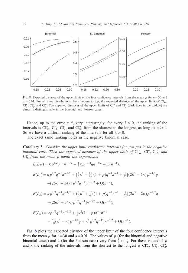
Fig. 8. Expected distance of the upper limit of the four con&dence intervals from the mean for n=30 and� = 0:01. For all three distributions, from bottom to top, the expected distance of the upper limit of CIW,CIuJ , CI

u2, and CI

uS. The expected distances of the upper limits of CI

uJ and CI

u2 (dark lines in the middle) are

almost indistinguishable in the binomial and Poisson cases.

Hence, up to the error n−2, very interestingly, for every �¿ 0, the ranking of theintervals is CIuW, CI

uJ , CI

u2, and CI

uS, from the shortest to the longest, as long as �¿ 1.

So we have a uniform ranking of the intervals for all �¿ 0.The exact same ranking holds in the negative binomial case.

Corollary 3. Consider the upper limit con2dence intervals for =p=q in the negativebinomial case. Then the expected distance of the upper limit of CIuW, CI

uJ , CI

u2, and

CIuS from the mean admit the expansions:

E(LW) = �p1=2q−1n−1=2 − 18�p

−1=2qn−3=2 + O(n−2);

E(LJ) = �p1=2q−1n−1=2 +(13�2 + 1

6

)(1 + p)q−1n−1 + 1

72 [(2�3 − 5�)p−1=2q

−(26�3 + 34�)p1=2q−1]n−3=2 + O(n−2);

E(L2) = �p1=2q−1n−1=2 +(13�2 + 1

6

)(1 + p)q−1n−1 + 1

72 [(2�3 − 2�)p−1=2q

−(26�3 + 34�)p1=2q−1]n−3=2 + O(n−2);

E(LS) = �p1=2q−1n−1=2 + 12�2(1 + p)q−1n−1

+[18 (�

3 − �)p−1=2q+ �3p1=2q−1]n−3=2 + O(n−2):

Fig. 8 plots the expected distance of the upper limit of the four con&dence intervalsfrom the mean for n=30 and �=0:01. The values of p (for the binomial and negativebinomial cases) and � (for the Poisson case) vary from 1

6 to13 . For these values of p

and � the ranking of the intervals from the shortest to the longest is CIuW, CIuJ , CI

u2,


and CIuS for all three distributions. In the cases of binomial and Poisson distributionsthe expected distances of CIuJ and CI

u2 are almost indistinguishable.

Considering together with the coverage properties discussed in the earlier sections,we can conclude that for all three distributions the expected distances of the upper limitof the Wald and score intervals are either too short or too long, which is not desirablein either case. The Je4reys and second-order corrected intervals are better alternatives.

6. One-sided hypothesis testing

The results on one-sided con&dence intervals discussed in the earlier sections havedirection implications on testing one-sided hypotheses. In the cases of the binomial,negative binomial and Poisson distributions the score test occupies a particularly impor-tant position in hypothesis testing. It is often the only test given in many introductorytextbooks. Due to the duality between the one-sided score interval and the one-sidedscore test, the fact that the one-sided score interval contains signi&cant systematic biasin the coverage probability implies that the actual size of the one-sided score test maybe far from the nominal level.Recall that in testing the one-sided hypotheses:

H0: ¿ 0 versus Ha: ¡0 (30)

at the signi&cance level �, the score test rejects the null hypothesis whenever

n1=2( KX − 0)V 1=2(0)

¡− �: (31)

The true size of the score test equals type I error probability under = 0, which isthe same as the non-coverage of the upper limit score interval 1− P0 (0 ∈CIuS).Fig. 9 plots the size of the upper limit score test at the nominal � = 0:01 level for

a binomial proportion, negative binomial mean, and Poisson mean with n = 30. It isclear that in all three cases the actual size not only oscillates as a function of , butcontains a serious systematic bias as well. In the binomial case, oscillations aside, the

p

0.2 0.4 0.6 0.8

p

0.2 0.4 0.6 0.8

lambda

0.5 1.0 1.5 2.0 2.5 3.0

0.0

0.005

0.010

0.015

0.020

0.025

0.0

0.005

0.010

0.015

0.020

0.025

0.0

0.005

0.010

0.015

0.020

0.025

Fig. 9. The size of the upper limit score test at nominal � = 0:01 level with n = 30. From left to right,binomial, negative binomial, and Poisson.


0.2 0.4 0.6 0.80.0

0.005

0.015

0.025

0.5 1.0 1.5 2.0 2.5 3.0

0.0

0.005

0.010

0.015

0.005

0.010

0.015

0.0

0.005

0.015

0.025

0.0

0.005

0.010

0.015

0.005

0.010

0.015

0.0

0.005

0.015

0.025

0.0

0.005

0.010

0.015

0.005

0.010

0.015

0.2 0.4 0.6 0.8

0.2 0.4 0.6 0.8

0.5 1.0 1.5 2.0 2.5 3.0

0.2 0.4 0.6 0.8

0.2 0.4 0.6 0.8

0.5 1.0 1.5 2.0 2.5 3.0

0.2 0.4 0.6 0.8

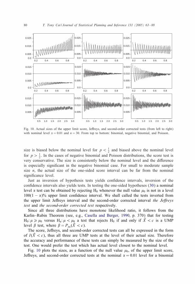
Fig. 10. Actual sizes of the upper limit score, Je4reys, and second-order corrected tests (from left to right)with nominal level � = 0:01 and n = 30. From top to bottom: binomial, negative binomial, and Poisson.

size is biased below the nominal level for p¡ 12 and biased above the nominal level

for p¿ 12 . In the cases of negative binomial and Poisson distributions, the score test is

very conservative. The size is consistently below the nominal level and the di4erenceis especially signi&cant in the negative binomial case. For small to moderate samplesize n, the actual size of the one-sided score interval can be far from the nominalsigni&cance level.Just as inversion of hypothesis tests yields con&dence intervals, inversion of the

con&dence intervals also yields tests. In testing the one-sided hypotheses (30) a nominallevel � test can be obtained by rejecting H0 whenever the null value 0 is not in a level100(1 − �)% upper limit con&dence interval. We shall called the tests inverted fromthe upper limit Je4reys interval and the second-order corrected interval the Je3reystest and the second-order corrected test respectively.Since all three distributions have monotone likelihood ratio, it follows from the

Karlin–Rubin Theorem (see, e.g., Casella and Berger, 1990, p. 370) that for testingH0: ¿ 0 versus Ha: ¡0 a test that rejects H0 if and only if KX ¡c is a UMPlevel / test, where / = P0 ( KX ¡c).The score, Je4reys, and second-order corrected tests can all be expressed in the form

of I( KX ¡c), thus all three are UMP tests at the level of their actual size. Thereforethe accuracy and performance of these tests can simply be measured by the size of thetest. One would prefer the test which has actual level closest to the nominal level.Fig. 10 plots the sizes, as a function of the null value 0, of the upper limit score,

Je4reys, and second-order corrected tests at the nominal �= 0:01 level for a binomial


proportion, negative binomial mean, and Poisson mean with n= 30. In comparison tothe score test, it is clear that overall the Je4reys and second-order corrected tests haveactual sizes much closer to the nominal signi&cance level.

7. Discussion and conclusions

7.1. The Clopper–Pearson interval

In the previous sections we give a uni&ed treatment of the one-sided con&denceintervals for the discrete Exponential family with a quadratic variance function whichconsists of the binomial, negative binomial, and Poisson distributions. In the case ofbinomial proportion, there is a well known “exact” interval, the Clopper–Pearson in-terval, which has received special attention.The one-sided Clopper–Pearson interval is the inversion of the one-sided binomial

test rather than its normal approximation. If X ∼ Bin(n; p) and X = x is observed,then the upper limit Clopper–Pearson interval (Clopper and Pearson, 1934) is de-&ned by CIuCP = [0; UCP(x)], where UCP(x), which is the solution in p to the equationPp(X 6 x) = �, equals the 1 − � quantile of a beta distribution Beta(x + 1; n − x).Similarly, the lower limit Clopper–Pearson interval is de&ned by CIlCP = [LCP(x); 1],where LCP(x), which is the solution in p to the equation Pp(X ¿ x) = �, equals the �quantile of a beta distribution Beta(x; n− x + 1).By construction, the Clopper–Pearson interval has guaranteed coverage probability

of at least 1−�. However, the actual coverage probability can be far above the nominallevel and the expected distance of the upper/lower limit from p is much larger thanthose of Je4reys or the second-order corrected intervals unless n is very large. Thereforethe Clopper–Pearson interval is too conservative and is not a good choice for practicaluse, unless strict adherence to the prescription that the coverage is at least 1 − � isrequired. Fig. 11 compares the coverage probability and the expected distance from pof the upper limit Clopper–Pearson and Je4reys intervals. The expected distance fromp of the upper limit of the Clopper–Pearson interval is about 12–18% larger than thatof the Je4reys interval.

7.2. Conclusions

We show through numerical and analytical calculations that the standard one-sidedWald interval and to a slightly lesser degree the one-sided score interval are uniformlypoor in the binomial, negative binomial, and Poisson distributions. The results show thatthe Je4reys and second-order corrected intervals provide signi&cant improvements overboth the Wald and score intervals. These two alternative intervals nearly completelyeliminate the systematic bias in the coverage probability. The one-sided Je4reys andsecond-order corrected intervals can be resolutely recommended. In testing one-sidedhypotheses, the actual size of the score test deviate systematically from the nominalsigni&cance level. The inversion of the Je4reys and second-order corrected intervals


0.2 0.4 0.6 0.8

0.90

0.92

0.94

0.96

0.98

1.00

C-P Interval

0.2 0.4 0.6 0.8

Jeffreys Interval

0.15 0.25 0.35

0.12

0.13

0.14

0.15

0.16

Expected Distance

0.90

0.92

0.94

0.96

0.98

1.00

Fig. 11. Coverage probability of the upper limit Clopper–Pearson interval (left panel) and the upper limitJe4reys interval (middle panel); expected distance from p of the upper limit Clopper–Pearson interval (rightpanel, dotted line) and the upper limit Je4reys interval (right, solid line) for a binomial proportion p withn = 30 and � = 0:05.

yields UMP tests which have actual sizes much closer to the nominal level. The Je4reysand second-order corrected tests are preferable to the one-sided score test.

Appendix A. Proofs

Except for the second-order corrected interval, most of the essential algebraic deriva-tion is similar to that given in Brown et al. (2002, 2003) for the two-sided con&denceintervals.All three distributions under consideration are lattice distributions with the maximal

span of one. Formulas of Edgeworth expansion for lattice distributions can be found,for example, in Esseen (1945) and Bhattacharya and Rao (1976). The following resultis from Brown et al. (2003).

Proposition 1. Let X1; X2; : : : ; Xniid∼F with F as one of the Bin(1; p), NBin(1; p), and

Poi(�) distributions. Denote Zn = n1=2( − )= and Fn(z) = P(Zn6 z). Then thetwo-term Edgeworth expansion of Fn(z) is given as

Fn(z) ="(z) + p1(z)!(z)n−1=2 − Q1(; z)−1!(z)n−1=2 + p2(z)!(z)n−1

+{Q1(; z)p3(z) + Q2(; z)}−2z!(z)n−1 + O(n−3=2); (A.1)

where Q1 and Q2 are given as in (12) and

p1(z) = 16 (1− z2)(1 + 2b∗)−1;

p2(z) =− 136 (2z

5 − 11z3 + 3z)b∗ − 172 (z

5 − 7z3 + 6z)−2;

p3(z) =− 16 (z

2 − 3)(1 + 2b∗)−1:


If z = z(n) depends on n and can be written as

z = z0 + c1n−1=2 + c2n−1 + O(n−3=2);

where z0; c1 and c2 are constants, then

Fn(z) ="(z0) + p1(z)!(z0)n−1=2 − Q1(; z)−1!(z)n−1=2 + p2(z)!(z0)n−1

+{Q1(; z)p3(z0) + Q2(; z)}−2z0!(z0)n−1 + O(n−3=2); (A.2)

where

p1(z) = c1 + 16 (1− z20)(1 + 2b∗)−1; (A.3)

p2(z) = c2 − 12 z0c

21 +

16 c1(z

30 − 3z0)(1 + 2b∗)−1 + p2(z0); (A.4)

p3(z) = c1 − 16 (z

20 − 3)(1 + 2b∗)−1: (A.5)

Remark. In (A.2), the second O(n−1=2) and the second O(n−1) terms are oscillationterms.

Proof of Theorems 1 and 4. We consider the coverage of a general upper limit intervalof the form:

CI∗ =[0;X + s1n− b∗s2 + �{V () + (r1V () + r2)n

−1}1=2n−1=2]; (A.6)

where s1, s2, r1 and r2 are constants. The con&dence intervals CIuW and CIu2 are special

cases of CI∗. Denote

A= n− b∗�2(1 + r1n−1)(1− b∗s2n−1)2;

B= 2n − 2(s1 + b∗s2) + �2(1 + r1n−1)(1− b∗s2n−1)2;

C = n( − (s1 + b∗s2)n−1)2 − r2�2n−1(1− b∗s2n−1)2:

By solving a quadratic equation, after some algebra, we have

P(∈CI∗) = P(n1=2( − )

¿ z∗

);

where

z∗ =

(B− √

B2 − 4AC2A

− )−1n1=2: (A.7)


Expanding z∗, one has

z∗ =−� − (s1 + b∗s2 − 12�2(1 + 2b∗))−1n−1=2 − {( 12 r1 + b∗�2 − b∗s2

)�

− 12�(s1 + b∗s2)(1 + 2b∗)

−2 +(12 r2� +

18�3) −2} n−1 + O(n−3=2):

(A.8)

Denote

c∗1 =−(s1 + b∗s2 − 12�2(1 + 2b∗))−1;

c∗2 =−{( 12 r1+b∗�2−b∗s2) �− 12�(s1+b∗s2)(1 + 2b∗)

−2+(12 r2�+

18�3) −2} :

Then z∗ = −� + c∗1n−1=2 + c∗2n−1 + O(n−3=2). It follows from (A.2) that the coeQ-cient of the O(n−1=2) non-oscillatory term in the Edgeworth expansion of the coverageP(∈CI∗) = 1− Fn(z∗) is

p∗1 (z∗) =−p1(z∗) =−c∗1 + 1

6 (�2 − 1)(1 + 2b∗)−1

={(s1 − ( 13�2 + 1

6

))+(s2 − 2 ( 13�2 + 1

6

))b∗}−1:

Thus, to make p∗1 (z∗) vanishing for all , one needs

s1 = 16 (2�

2 + 1) and s2 = 13 (2�

2 + 1) (A.9)

With s1 and s2 given as in (A.9), one has

c∗2 =− 12�r1 +

13 (�

3 + 2�)b∗ − 12�

−2r2 + 124 (�

3 + 2)−2:

It follows from (A.4) that the coeQcient of the O(n−1) non-oscillatory term in theEdgeworth expansion of P(∈CI∗) is

p∗2 (z∗) =−p2(z∗) =−c∗2 − 1

36 (�3 − 7�)b∗ + 1

72 (�3 − �)−2

= 12�{r1 − 1

18 (13�2 + 17)b∗

}+ 1

2�−2 {r2 − 1

36 (2�2 + 7)

}:

Therefore we choose

r1 = 118 (13�

2 + 17)b∗ and r2 = 136 (2�

2 + 7) (A.10)

to make the O(n−1) non-oscillatory term vanishing.

• For the standard interval, we have zW de&ned as in (A.7) with s1=s2=r1=r2=0.From (A.8) we have

zW =−� + 12�2(1 + 2b∗)−1n−1=2 − (b∗ + 1

8−2)�3n−1 + O(n−3=2):

Now, P(∈CIuW) = 1− Fn(zW) and (14) follows from (A.2).• For the second-order corrected interval, we have z2 de&ned as in (A.7) withs1 = 1

6 (2�2 + 1), s2 = 2s1, r1 = 1

18 (13�2 + 17)b∗, and r2 = 1

36 (2�2 + 7). It follows


from (A.8) that

z2 =−� + 16(�

2 − 1)(1 + 2b∗)−1n−1=2

−{ 118 (7�3 + 5�)b∗ − 172 (�

3 − �)−2)}n−1 + O(n−3=2):

Now (17) follows from (A.2).

Proof of Theorem 2. The Edgeworth expansion for P(∈CIuS) is simple because

PS = P(∈CIuS) = P(n1=2( − )

¿− �

):

And now (15) follows from (A.1).

A.1. Expansion for Je3reys prior intervals

We now prove Theorem 3. Denote the cdf of the posterior distribution of 3 (3= pin the binomial and negative binomial case and 3=� in the Poisson case) given X = xby F(·; x; n) and denote by B(�; x; n) the inverse of the cdf. Then

P(3∈CIuJ ) = P(36B(1− �;X; n)) = P(F(3;X; n)6 1− �):

Holding other parameters &xed, the function F(3; x; n) is strictly decreasing in x in allthree cases. So there exist a unique Zl = 4(1− �; 3) satisfying

F(3;Zl; n)6 1− � and F(3;Zl − 1; n)¿ 1− �:

Therefore

P(3∈CIuJ ) = P(n1=2( KX − )

¿ zJ

)

with

zJ = (4(1− �; 3)− n)−1n−1=2 (A.11)

Here zJ is de&ned implicitly in (A.11) through 4. The proof of (16) requires an asymp-totic expansion for zJ. Using (A.29) in Brown et al. (2002) for the binomial case, and(56) and (65) in Brown et al. (2003) respectively for the negative binomial and thePoisson case, we have a uni&ed expression for the approximation of zJ:

zJ =−� + 16(�

2 − 1)(1 + 2b∗)−1n−1=2

− 172{(2�3 − 14�)b∗ − (�3 + 2�)−2}n−1 + O(n−3=2): (A.12)

Now we can obtain expansion (16) by plugging in (A.12) into (A.2).


A.2. Expansions for expected distance from the mean

We now prove Theorem 5. Denote below Zn = ( KX − )( + b∗2)−1=2n1=2. ThenE(Zn) = 0 and E(Z2n ) = 1.

The interval CIuW: The expected distance of the upper limit of the Wald intervalCIuW from the mean is

LW = KX + �( KX + b∗ KX 2)1=2n−1=2 − = Zn( + b∗2)1=2n1=2

+�( + b∗2)1=2n−1=2(1 + Zn(1 + 2b∗)( + b∗2)−1=2n−1=2 + b∗Z2nn−1)1=2;

on some algebra by using the de&nition of Zn. Hence,

LW = Zn(+b∗2)1=2n1=2+�(+b∗2)1=2n−1=2+12�Zn(1 + 2b∗)n

−1

− 18Z

2n (+b∗

2)−1=2�n−3=2+RW(Zn); (A.13)

where E(|RW(Zn)|)=O(n−2). see Brown et al. (2002) for more details. Now expansion(22) follows from (A.13) on some algebra.

The interval CIuS: For the Rao score interval CIuS, the distance is

LS = ( KX+12�2)(1−b∗�2n−1)−1+�(1−b∗�2n−1)−1( KX+b∗ KX 2+1

4�2n−1)1=2n−1=2−

= 12(1+2b∗)�

2n−1+Zn(+b∗2)1=2n−1=2+�( + b∗2)1=2(1 + b∗�2n−1)n−1=2

+ 12�Zn(1 + 2b∗)n

−1 + 18 (�

3 − �)( + b∗2)−1=2Z2nn−3=2 + RS(Zn);where exactly as in (A.13) above, E(|RS(Zn)|) = O(n−2). Thus

E(LS) = 12 (1 + 2b∗)�

2n−1 + �( + b∗2)1=2(1 + b∗�2n−1)n−1=2

+18 (�

3 − �)( + b∗2)−1=2n−3=2 + O(n−2)which yields expressions (25) and (29).

The interval CIu2: Using the de&nition of Zn,

= ( + Zn( + b∗2)1=2n−1=2 + �n−1)(1− 2�b∗n−1)−1

and hence, after some algebra,

L2 = (1 + 2b∗)�n−1 + Zn(1 + 2�b∗n−1)( + b∗2)1=2n−1=2

+�(1 + 12�1n

−1)( + b∗2)1=2n−1=2 + 12�Zn(1 + 2b∗)n

−1

− 18�Z

2n ( + b∗

2)−1=2n−3=2 + 12��2( + b∗

2)−1=2n−3=2 + R2(Zn); (A.14)

where E(|R2(Zn)|) = O(n−2). Thus, &nally, from (A.14),

E(L2) = (1 + 2b∗)�n−1 + �(1 + 12�1n

−1)( + b∗2)1=2n−1=2

− 18�( + b∗

2)−1=2n−3=2 + 12��2( + b∗

2)−1=2n−3=2 + O(n−2)

which simpli&es to Eq. (28) on a few steps of algebra.


The interval CIuJ : The upper limit of CIuJ admit the general representation

KX + w1( KX )n−1 + {�( KX + b∗ KX 2)1=2n−1=2 + w2( KX )n−3=2}+ RJ(n);where the remainder RJ(n) satis&es E(|RJ(n)|) = O(n−2), and

w1() = 16 (2�

2 + 1)(1 + 2b∗);

w2() = 136 ( + b∗

2)−1=2{(�3 + 3�) + b∗( + b∗2)(13�3 + 17�)}:Thus, directly, the distance LJ of CIuJ satis&es

E(LJ) = 16 (2�

2 + 1)(1 + 2b∗)n−1

+E[�( KX + b∗ KX 2)1=2n−1=2 + w2( KX )n−3=2] + O(n−2)

= �( + b∗2)1=2n−1=2 + 16 (1 + 2b∗)(2�

2 + 1)n−1

− 18�( + b∗

2)−1=2n−3=2 + w2()n−3=2 + O(n−2)

which yields expressions (24) and (27) after some algebra.

References

Agresti, A., Coull, B.A., 1998. Approximate is better than “exact” for interval estimation of binomialproportions. Amer. Statist. 52, 119–126.

Berger, J.O., 1985. Statistical Decision Theory and Bayesian Analysis, 2nd Edition. Springer, New York.Bhattacharya, R.N., Rao, R.R., 1976. Normal Approximation And Asymptotic Expansions. Wiley, New York.Blyth, C.R., Still, H.A., 1983. Binomial con&dence intervals. J. Amer. Statist. Assoc. 78, 108–116.Brown, L.D., 1986. Fundamentals of Statistical Exponential Families with Applications in Statistical DecisionTheory, Lecture Notes-Monograph Series, Institute of Mathematical Statistics, Hayward.

Brown, L.D., Cai, T., DasGupta, A., 2001. Interval estimation for a binomial proportion (with discussion).Statist. Sci. 16, 101–133.

Brown, L.D., Cai, T., DasGupta, A., 2002. Con&dence intervals for a binomial proportion and Edgeworthexpansions. Ann. Statist. 30, 160–201.

Brown, L.D., Cai, T., DasGupta, A., 2003. Interval estimation in exponential families. Statist. Sinica 13,19–49.

Cai, T., 2003. One-sided con&dence intervals in discrete distributions. Technical Report, Department ofStatistics, University of Pennsylvania.

Casella, G., Berger, R.L., 1990. Statistical Inference. Wadsworth, Brooks Cole, CA.Clopper, C.J., Pearson, E.S., 1934. The use of con&dence or &ducial limits illustrated in the case of thebinomial. Biometrika 26, 404–413.

Cressie, N., 1980. A &nely tuned continuity correction. Ann. Inst. Statist. Math. 30, 435–442.Duncan, A.J., 1986. Quality Control and Industrial Statistics, 5th Edition. Irwin, Homewood, IL.Esseen, C.G., 1945. Fourier analysis of distribution functions: a mathematical study of the Laplace–Gaussianlaw. Acta Math. 77, 1–125.

Ghosh, J.K., 1994. Higher Order Asymptotics. NSF-CBMS Regional Conference Series, Institute ofMathematical Statistics, Hayward.

Ghosh, M., 2001. Comment on “Interval estimation for a binomial proportion” by L. Brown, T. Cai and A.DasGupta. Statist. Sci. 16, 124–125.

Hall, P., 1982. Improving the normal approximation when constructing one-sided con&dence intervals forbinomial or Poisson parameters. Biometrika 69, 647–652.

Montgomery, D.C., 2001. Introduction to Statistical Quality Control, 4th Edition. John Wiley, New York.


Morris, C.N., 1982. Natural exponential families with quadratic variance functions. Ann. Statist. 10, 65–80.Newcombe, R.G., 1998. Two-sided con&dence intervals for the single proportion; comparison of severalmethods. Statist. Med. 17, 857–872.

Santner, T.J., 1998. A note on teaching binomial con&dence intervals. Teaching Statistics 20, 20–23.Vollset, S.E., 1993. Con&dence intervals for a binomial proportion. Statist. Med. 12, 809–824.

Documents

One-sidedcondenceintervalsindiscrete …tcai/paper/1sidedCI.pdfOne-sidedcondenceintervalsindiscrete distributions T.TonyCai ∗ Department of Statistics, The Wharton School, University