Embed Size (px)
Citation preview
Performance Evaluation 00 (2010) 1–24
PerformanceEvaluation
Online Anomaly Detection for Sensor Systems: a Simple andEfficient Approach
Yuan Yaoa, Abhishek Sharmab, Leana Golubchika,b, Ramesh Govindanb
aDepartment of Electrical Engineering-Systems, USC, Los Angeles, CA 90089bDepartment of Computer Science, USC, Los Angeles, CA 90089
Abstract
Wireless sensor systems aid scientific studies by instrumenting the real world and collectingmeasurements. Given the large volume of measurements collected by sensor systems, one prob-lem arises – an automated approach to identifying the “interesting” parts of these data sets, oranomaly detection. A good anomaly detection methodology should be able to accurately iden-tify many types of anomalies, be robust, require relativelylittle resources, and perform detectionin (near) real-time. Thus, in this paper we focus on an approach to online anomaly detectionin measurements collected by sensor systems, where our evaluation, using real-world datasets,shows that our approach is accurate (it detects over 90% of the anomalies with few false posi-tives), works well over a range of parameter choices, and hasa small (CPU, memory) footprint.
Keywords: anomaly detection, sensor systems, real-world deployments.
1. Introduction
Wireless sensor systems have significant potential for aiding scientific studies by instrument-ing the real world and collecting measurements, with the aimof observing, detecting, and track-ing scientific phenomena that were previous only partially observable or understood. However,one obstacle to achieving the full potential of such systems, is the ability to process, in a timelyand meaningful manner, the huge amounts of measurements they collect. Given such large vol-umes of collected measurements, one natural question mightbe: Can we devise an efficientautomated approach to identifying the “interesting” partsof these data sets?For instance, con-sider a marine biology application collecting fine-grainedmeasurements in near real-time (e.g.,temperature, light, micro-organisms concentrations) – one might want to rapidly identify “ab-normal” measurements that might lead to algal blooms which can have devasting consequences.
Email addresses:[email protected] (Yuan Yao),[email protected] (Abhishek Sharma),[email protected](Leana Golubchik),[email protected] (Ramesh Govindan)
/ Performance Evaluation 00 (2010) 1–24 2
We can view identification of such “interesting” or “unexpected” measurements (or events) incollected data as anomaly detection. In the remainder of thepaper, we use the generic term“anomaly” for all interesting (typically, other-than-normal) events occurring either on the mea-sured phenomena or the measuring equipment. Automatedonline (or near real-time) anomalydetection in measurements collected by sensor systemsis the focus of this paper.
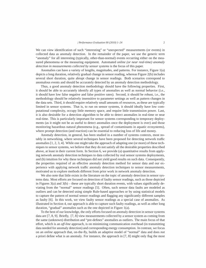
Anomalies can have a variety of lengths, magnitudes, and patterns. For instance, Figure 1(a)depicts a long duration, relatively gradual change in sensor reading, whereas Figure 2(b) includesseveral short duration, quite abrupt change in sensor readings. Both scenarios correspond toanomalous events and should be accurately detected by an anomaly detection methodology.
Thus, a good anomaly detection methodology should have the following properties. First,it should be able to accurately identify all types of anomalies as well as normal behavior (i.e.,it should have low false negative and false positive rates).Second, it should be robust, i.e., themethodology should be relatively insensitive to parametersettings as well as pattern changes inthe data sets. Third, it should require relatively small amounts of resources, as these are typicallylimited in sensor systems. That is, to run on sensor systems,it should ideally have low com-putational complexity, occupy little memory space, and require little transmission power. Last,it is also desirable for a detection algorithm to be able to detect anomalies in real-time or nearreal-time. This is particularly important for sensor systems corresponding to temporary deploy-ments (as it might not be as useful to detect anomalies once the deployment is over) and thosemonitoring hazardous natural phenomena (e.g., spread of contaminants in aquatic ecosystems),where prompt detection (and reaction) can be essential to reducing loss of life and money.
Anomaly detection, in general, has been studied in a number of systems contexts, most no-tably in networking, where several techniques have been proposed for detecting network trafficanomalies [1, 2, 3, 4]. While one might take the approach of adapting one (or more) of these tech-niques to sensor systems, we believe that they do not satisfyall the desirable properties describedabove, at least in their current form. In Section 6, we provide (a) quantitative results from apply-ing network anomaly detection techniques to data collectedby real sensor systems deployments,and (b) intuition for why these techniques did not yield goodresults on such data. Consequently,the properties required of an effective anomaly detection method for sensor data and our ex-perience with applying network traffic anomaly detection techniques to sensor measurements,motivated us to explore methods different from prior work in network anomaly detection.
We also note that little exists in the literature on the topicof anomaly detection in sensor sys-tems data. Most efforts are focused on detection of faulty sensor readings, such as those depictedin Figures 3(a) and 3(b) – these are typically short durationevents, with values significantly de-viating from the “normal” sensor readings [5]. Often, such sensor data faults are modeled asoutliers and can be detected using simple Rule-based approaches or by using statistical modelsto capture the pattern of normal sensor readings and flaggingany significantly different samplesas faulty [6]. In this work, we view faulty sensor readings asa special case of anomalies. Asillustrated in Section 4, our approach is able to capture such faulty readings, as well as other longduration, “gradual” anomalies such as the one depicted in Figure 1(a).
To the best of our knowledge, the only efforts focused on anomaly detection in sensor systemsdata are [7, 8, 9]. Briefly, [7, 8] view measurements collected by a sensor system as coming fromthe same (unknown) distribution and “pre-defines” anomalies as outliers. The main focus of thateffort, which is anoff-line approach, is on minimizing communication overhead (in transmittingdata needed for anomaly detection) and corresponding energy consumption. In contrast, we focuson anonlineapproach that, on-the-fly, builds an adaptive model of “normal” data and doesnota priori define what is an anomaly. For instance, the approachin [7, 8] might only flag the most
/ Performance Evaluation 00 (2010) 1–24 3
extreme measurement in Figure 1(a) as an anomaly, whereas our approach would flag the entireevent (outlined by the dashed rectangle) as an anomaly We give a more detailed descriptionof [7, 8] and a quantitative comparison in Section 6. In [9] a change point detection basedapproach is used for detecting distribution changes (e.g.,mean, variance, covariances) in sensormeasurements. However, (a) this approach assumes knowledge of the (time varying) probabilitydistribution from which sensor measurements are sampled (information often not available inreal-world deployments), and (b) such techniques do not meet (at least in their current form) ourefficiency criteria (see Section 6).
1000 2000 3000 4000 5000 6000−5
0
5
10
Sample Number
Tem
pera
ture
275 290 302
4.9
5
5.1
5.2
Sample Number
Tem
pera
ture
X(j)
Y(j)
Y(j+1)
X(j+1)
(a) Long duration anomaly (b) Piecewise linear model for time series data
Figure 1: (a) Data set with long duration anomaly and (b) example of a piecewise linear model.
In this work, we formulate the problem of anomaly detection in sensor systems as an instanceof identifying unusual patterns in time series data problem. Of course, one possible directionwould then be to construct a timeseries-based approach, e.g., based on [6]. However, we also didnot find this direction to be effective as such techniques are (typically) not well-suited for detect-ing long duration anomalies. So, we do not pursue this direction further here, but in Section 6,we do illustrate quantitative results corresponding to applying a representative timeseries-basedapproach to data collected by real sensor systems deployments and provide intuition for whysuch a technique did not yield good results.
In contrast, the basic idea behind our approach is to comparethe collected measurementsagainst a reference time series. But, to do this efficiently and robustly, the following challengingproblems need to be solved: (1) How do define a reference time series?; (2) How to compare twotime series efficiently?; (3) What metric to use in deciding whether two sensor data time seriesare similar or different?; and (4) How to update the reference time series, to adapt to (normal)changes in sensor data patterns?
We address these challenges by proposing and evaluating an anomaly detection algorithm,termed Segmented Sequence Analysis (SSA) that exhibits thedesirable characteristics statedabove. Briefly, SSA leverages temporal and spatial correlations in sensor measurements andconstructs a piecewise linear model of sensor data time series. This is motivated by [10] whichfocused on searching forknown patternsin time series (see Section 6). To detect anomalies,we compare the piecewise linear models of sensor data (collected during a time interval) anda reference model, with significant differences (as determined by a proposed similarity metric)flagged as anomalies. We use data from real-world deployments to evaluate our approach anddemonstrate its accuracy, robustness, and efficiency. In summary, our the main contributions are:
• We propose an approach to anomaly detection in sensor systems that is able to detectanomalies accurately and in anonlinemanner (Section 2).

/ Performance Evaluation 00 (2010) 1–24 4
• We perform an extensive study using data sets from two real deployments, one consistingof about 30,000 environmental temperature measurements collected by 23 sensor nodesfor around 43 days, and the other consisting of more than 10,000 soil temperature, mois-ture, and air humidity measurements collected by 3 sensor nodes for over 5 months. Thisstudy illustrates that our approach is accurate (it detectsover 90% of the anomalies withfew false positives), works well over a range of parameter choices, and has a small (CPU,memory) footprint (Sections 3 and 4).
• We show that our (online) SSA-based based approach is more accurate than potential other(offline) techniques1, which are more computationally intensive (Section 5 and 6).
2. Methodology
In this section, we first describe a tiered sensor system architecture that is representative ofdata collection deployments. We then formulate the problemof anomaly detection in sensorreadings as an instance of the problem of identifying unusual patterns in time series data. Lastly,we describe our method for detecting anomalous sensor readings.
2.1. Sensor systems for data collection
We consider a typical tiered sensor system [11] consisting of two tiers: a lower-tier ofresource-constrained battery-operated wirelessmoteswith one or more attached sensors (e.g.,temperature, humidity, acceleration), and an upper tier ofmore capablemasternodes each ofwhich has significantly higher computation, storage, and communication capabilities than themotes. Here, we are interested in the class of data collection sensor systems, where each mote(usually) collects periodic sensor data, possibly performs some local processing on the data, andthen transfers the resulting data over multiple hops. We model the measurements collected bya sensorm as a time seriesDm[t], t = 1,2, . . .. For example, suppose a sensing system had 20motes, each collecting data from 3 sensors. Then, we would have a total of 60 time series (3 fromeach of the 20 motes), and we would represent these as a set{Dm[t],m= 1,2, . . . ,60;t = 1,2, . . .}.
In many data collection applications, these time series exhibit a high degree of temporaland spatial correlations due to the nature of the physical phenomenon being monitored (e.g.,temperature or light conditions). We leverage such correlations to detect anomalies (interestingevents) in the sensor data time series. As noted in Section 1,anomalies have various lengths,magnitudes, and patterns, and a good anomaly detection methodology should be robust to suchvariations.
We first describe the building blocks of our approach, where the basis involves building (andcontinuously updating) a model of the “normal” and then determining how similar new sensormeasurements are to the “normal”. We then describe our approach to anomaly detection.
2.2. Building blocks
At a high level, our approach answers the following question: How similar is a time seriesof sensor measurements to a given “reference” time series?. Suppose we are given two timeseries,Dnew[t] and Dre f [t], where Dnew[t] is the time series of new sensor data, andDre f [t]
1Most of these were designed in other contexts, but constitute possible directions that could have been taken forsensor systems anomaly detection.
/ Performance Evaluation 00 (2010) 1–24 5
is the reference time series. Then, an anomaly detection method can: (1) Construct modelscorresponding toDnew[t] andDre f [t]; (2) Compare these two models using a similarity measure;and (3) If the model forDnew[t] is not sufficiently similar to the model forDre f [t], conclude thatthere are anomalies in the time seriesDnew[t]. Thus, our method involves solving three mainproblems: (1) how to construct the models forDnew[t] andDre f [t], (2) which similarity measureto use for comparing these models, and (3) how to decide whether the models for two differenttime series data are sufficiently similar, given our similarity measure.
Piecewise linear model. We use a piecewise linear model to representDnew[t] and Dre f [t].Figure 1(b) depicts an example piecewise linear representation of sensor measurements collectedby the SensorScope deployment [12]. Each line segment represents a small subset of sensorreadings, determined using linear least-squares regression. The advantages of a piecewise linearrepresentation of time series data are: (a) It issuccinct, since only a few line segments are neededto represent a large amount of time series data; (b) It isrepresentativeas essential information(e.g., significant patterns) in the data is captured; (c) It is robustto changes in model parametersas well as to faults and noise in sensor measurements (as demonstrated in Section 4).
A succinct, representative, and robust piecewise linear model of sensor data time series isdesirable foronline anomaly detection. First, we can compute such a model in nearreal-time(Section 2.3). Second, it enables us to create adata drivenreference model that is easy toupdate – hence, we do not need prior knowledge about the typesof anomalies that sensor datamight contain. Third, because it is succinct, it enables us to compare two different time seriesefficiently and transmit models with low overhead. Finally, because it is representative of thesensor datapatterns, it enables accurate detection of anomalous patterns.
Due to their usefulness in modeling time series data, linearization based approaches havealso been used in other contexts. For example, [10] developed an efficient technique to searchfor occurrences of aknown patternwithin a time series. However, the problem of searching fora known pattern in time series data is different from anomaly detection because often we do nothave any prior information about the patterns exhibited by anomalous sensor readings.
Linearization Error. In order to compute a piecewise linear model, we need to definethelinearization errorbetween a sensor data pointj and the line segmentl covering it. We define thiserror as the perpendicular distance between the pointj and the linel. Accordingly, we define thelinearization errorǫ for a piecewise linear model representing a time series{D[t], t = 1,2,3...,n},as the maximum linearization error across all the data points in D[t].
How many line segments to use?We also need to determine the number of line segments,k,to use. Intuitively, using a large number of line segments will result in a small linearization error– as explained below, this leads to lower computation cost but larger communication cost. (Thistradeoff is explored in detail in Section 4.2.)
We automatically determine the number of line segments in our piecewise linear model basedon the maximum allowed linearization errorǫ, which is a (free) parameter in our approach. Fora fixed choice of maximum linearization errorǫ, we use agreedyapproach to determine thenumber of line segments needed to represent a time series. Westart with the first two data pointsof the time series and fit a line segment, (say)l1, to them. Then we consider the data points oneat a time and recomputel1 using linear least-squares regression to cover a new data point. Wecompute the distance of the new data point from the linel1. If this distance is greater thanǫ,then we start a new line segment,l2 such that the distance between the new data point andl2 is atmostǫ. We keep repeating this process until we exhaust all data points. Note that our approach
/ Performance Evaluation 00 (2010) 1–24 6
is suited for bothofflineandonlineprocessing. In anonlinesetting, whenever the sensor collectsa new reading, we can either recompute the current line segment to cover it or start a new linesegment (depending on the linearization error).
We represent thek line segments that constitute a piecewise linear model of a time seriesusing their end points{(X[i],Y[i]), i = 1,2, . . . , k}, whereX[i] denotes a sample number (or thetime at which a sample was collected). The correspondingY[i] is one of the end points of aline segment and represents an estimate of the actual sensorreading collected at timeX[i]. Forexample, in Figure 1(b), the line segments approximate actual sensor readings (shown using dots)– here we indicate two measurement collection times,X[ j] andX[ j + 1] that correspond to twoend points,Y[ j] andY[ j + 1], that are part of a piecewise linear model.
Similarity measure. Let {(X[i], Y[i]), i = 1,2, . . . , k} and{(X[i], Y[i]), i = 1,2, . . . , k} denotethe piecewise linear representation of two time seriesD[t] and D[t], respectively. In order todefine a similarity measure between any two piecewise linearrepresentations, we need to firstalign them so that theirX[i] values (end points on the x-axis) line up. For example, considertwo representations{(X[i], Y[i]), i = 1,2} and{(X[i], Y[i]), i = 1,2,3} such thatX[1] = X[1] andX[3] = X[2], and hence,X[2] < X[2]. In order to align the two representations, we choose theXvalues as{X[1] = X[1] = X[1],X[2] = X[2],X[3] = X[2] = X[3]}. Hence, after alignment, thenew representations are{(X[i], Y[i]), i = 1,2,3}, and{(X[i],Y[i]), i = 1,2,3}, whereY[1] = Y[1],Y[3] = Y[2] and theY[2] value (corresponding to the sample at timeX[2]) is computed using theequation of the line segment joiningY[1] andY[3].
We define thedifferencebetween the (aligned) piecewise linear representations oftwo timeseriesD[t] andD[t] as:
S(D, D) =1k
k∑
i=1
|Y[i] − Y[i]| (1)
Here,S(D, D) represents the average difference between theY values of the piecewise linearrepresentations ofD[t] and D[t] over thek line segments. We chose this metric because it isefficient to compute, and it indirectly captures the difference between the two time series.
Threshold computation. We set the thresholdγ (for deciding whetherS(D, D) is sufficientlylarge) to the standard deviation of theinitial D re f [t]. We remove any CONSTANT anomalies (de-scribed in Section 3), before computing the standard deviation - intuitively such measurementsare not a good indication of variability in sensor data as they typically correspond to faulty data,e.g., due to low voltage supply to the sensor [5]. Intuitively, the standard deviation is a reasonableindication of the variability in the “normal” data. A multiple of standard deviation could alsobe used, but our more conservative approach already results(Section 3) in a reasonably low falsepositive rate; more sophisticated (than threshold-based)approaches are part of future efforts.
Putting it all together. Given a time series of new sensor data,Dnew[t], and a reference timeseries,Dre f [t], our Segmented Sequence Analysis (SSA) based approach to anomaly detectionutilizes the following steps (all detailed above):
1. Linearization: We apply our linearization technique to obtain the two piecewise linearmodels{(Xnew[i],Ynew[i])} and{(Xre f [i],Yre f [i])}.
2. Alignment: We align the two linear representations so that they have the sameX values.3. Similarity computation: We compute the similarity,S(Dnew,Dre f ), between the reference
model and the model for new sensor data using Equation (1).
/ Performance Evaluation 00 (2010) 1–24 7
4. Anomaly detection: We detect an anomaly using a simple threshold-based approach.Specifically, ifS(Dnew,Dre f ) is greater than a thresholdγ, then we conclude that the sensorreadingsDnew[t] contain an anomaly.
We now describe in detail our SSA-based anomaly detection framework.
2.3. UsingSSAon a tiered sensor network
We perform anomaly detection in a tiered sensor network in two stages – (1) alocal step,executed at each mote, followed by (2) anaggregationstep, executed at the master nodes. In thelocal step we exploit temporal correlations (in sensor readings), and in the aggregation step weexploit spatial correlations, as described next.
Local step. During the local phase (executed at individual motes), each motemperforms thefollowing tasks: (1) construct or update a reference time series,Dre f
m [t], for its sensor readings,(2) collect new sensor readings{Dnew
m [t], t = 1,2, . . . ,T} over a periodT, (3) construct or updatelinear models forDnew
m [t] and Dre fm [t], and (4) perform anomaly detection using the SSA-based
method (refer to Section 2.2).
Reference time series. To construct a reference time series at motem, Dre fm [t], we use the
following approach. For physical phenomena such as ambienttemperature or humidity variationsthat exhibit a diurnal pattern, we initially start with a time seriesD[t] consisting of measurementscollected over a period of 24 hours, (say) on day 1 of the deployment. LetDnew[t] be the newsensor readings collected by motemover time periodT corresponding to (say) 9-9:30 a.m. on day2 of the deployment. For these new readings, we define the datapoints inD[t] that were collectedbetween 9-9:30 a.m. (on day 1) asDre f [t]. We first look for anomalies in the new sensor readingsDnew[t], and then use the data points inDnew[t] to updateDre f [t] using weighted averaging. Forexample, we can use exponential weighted moving averaging to (pointwise) updateDre f [t], i.e.,Dre f [t] = (1−α)×Dre f [t] +α×Dnew[t], whereDre f [t] denotes the updated reference time series.
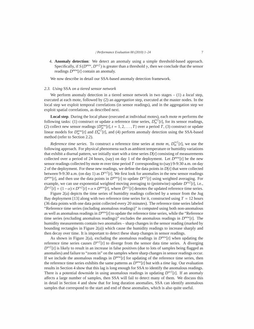
Figure 2(a) depicts the time series of humidity readings collected by a sensor from the JugBay deployment [13] along with two reference time series forit, constructed usingT = 12 hours(36 data points with one data point collected every 20 minutes). The reference time series labeled“Reference time series (including anomalous readings)” iscomputed using both non-anomalousas well as anomalous readings inDnew[t] to update the reference time series, while the “Referencetime series (excluding anomalous readings)” excludes the anomalous readings inDnew[t]. Thehumidity measurements contain two anomalies – sharp changes in the sensor reading (marked bybounding rectangles in Figure 2(a)) which cause the humidity readings to increase sharply andthen decay over time. It is important to detect these sharp changes in sensor readings.
As shown in Figure 2(a), excluding the anomalous readings inDnew[t] when updating thereference time series causesDre f [t] to diverge from the sensor data time series. A divergingDre f [t] is likely to result in an increase in false positives (due tolots of samples being flagged asanomalies) and failure to “zoom in” on the samples where sharp changes in sensor readings occur.If we include the anomalous readings inDnew[t] for updating of the reference time series, thenthe reference time series exhibits the same patterns asDnew[t] but with atime lag. Our evaluationresults in Section 4 show that this lag is long enough for SSA to identify the anomalous readings.There is a potential downside in using anomalous readings inupdatingDre f [t]. If an anomalyaffects a large number of samples, then SSA will fail to detect many of them. We discuss thisin detail in Section 4 and show that for long duration anomalies, SSA can identify anomaloussamples that correspond to the start and end of these anomalies, which is also quite useful.
/ Performance Evaluation 00 (2010) 1–24 8
For scenarios where the “normal” pattern of sensor readingsmight not be known or mightnot exhibit any periodicity – e.g., sensors deployed for monitoring of birds’ nests [11], in theabsence of any domain expertise, we assume that the sensor readings collected over a largeduration (a 24 hour period in most cases) capture the normal patterns in the sensor data timeseries, and start with such a time series as our reference. Clearly, the performance of our localanomaly detection step depends on the quality of the reference data. A reference data that doesnot capture the normal sensor readings or is corrupted by anomalies can lead to false positivesand/or false negatives. In Section 4, using real-world sensor readings for periodic (e.g., ambienttemperature) as well as aperiodic (e.g., soil moisture variations) phenomena, we show that ourapproach for selecting and updatingDre f
m [t] is robust and works well in practice.
Aggregation step. After performing its local step, each motem sends its linear model,{(Xnew
m [i],Ynewm [i]), i = 1, ., k}, for the new sensor readings,Dnew
m [t], and the results of its localanomaly detection step to its master node. For each motem, the master node performs anotherround of anomaly detection by comparing its linear model against the models from other motes(treating them as reference). Hence, a master node managingn slave motes performsO(n2)model comparisons. The design of our aggregation step is based on the observations from severalreal-world deployments that often the readings from sensors deployed at different locations arecorrelated [12]. The aggregation step exploits these spatial correlations to detect additionalanomalies (if any) that might not have been detected during the local step.
The final set of anomalies is the union of the anomalies detected during the local and aggre-gation steps. In our current framework, the master node doesnot provide feedback to its slavemotes. Hence, the anomalous readings from motem detected only by the aggregation step arecurrently not leveraged to improve the accuracy of the localanomaly detection step. Incorporat-ing a feedback mechanism between the aggregation and local steps is part of future efforts.
Online fault detection. To achieve online detection, we run the local and aggregationanomaly detection steps periodically, everyT minutes. For example, ifT = 30 min, we firstcollect new sensor readings for half an hour and then performanomaly detection using theframework described above. The anomaly detection interval, T, controls the trade-off betweenreal-time anomaly detection and resource consumption, as discussed in detail in Section 4.2.
2500 3000 3500 4000 4500 5000 55000
20
40
60
80
100
Sample Number
Hum
idity
Sensor readingsReference (including anomalous readings)Reference (excluding anomalous readings)
Anomalies
2000 3000 4000 5000 6000 7000 8000 9000−5
0
5
10
Tem
pera
ture
2000 4000 6000 8000Normal
Abnormal
Sample Number
SHORT Anomaly
(a) Reference time series (b) Short anomalies (marked by rectangles)
Figure 2: Examples of Anomalies in Sensor Readings
2.4. Hybrid approachAs noted in Section 2.2, our piecewise linear representation is very succinct – in practice, a
small number of line segments is sufficient to capture the essential information (diurnal patterns,
/ Performance Evaluation 00 (2010) 1–24 9
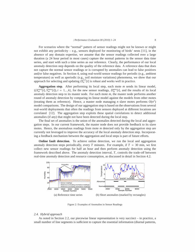
trends lasting for a long duration, etc.) in a time series. However, because it is designed tocapture significant trends, a piecewise linear representation will mask faults or anomalies thataffect a very small number of sensor samples. The top plot in Figure 2(b) shows a temperaturereading time series from the SensorScope datasets [12], andthe bottom plot shows whether eachsensor reading was identified as “normal” or “anomalous” by SSA. While SSA is able to detectinstances of long duration anomalies (marked by circles) itfails to detect the three very shortduration anomalies (marked by rectangles in the top plot). To improve the accuracy of SSA onshort duration anomalies, next we propose ahybrid approach.
Combining SSA with Rule-based methods. We can view data faults in sensor readingsas short duration anomalies (refer to Section 6). Thus, it isreasonable to adapt techniques de-signed for fault detection for identification of short duration anomalies. Specifically, [14, 6] arerepresentative of such techniques and they consider: SHORTanomalies (a sharp change in themeasured sensor readings between two successive samples),NOISE anomalies (increase in thevariance of sensor readings) and CONSTANT or “Stuck-at” anomalies (the sensor reports a con-stant value). Thus, we use the Rule-based methods [6] (originally designed for fault detection),for detection of short range anomalies in our hybrid approach by adding the following rules.
SHORT Rule: To detect SHORT anomalies in the time series{D[t], t = 1,2,3...}, we keeptrack of the change in sensor readings between two successive samples,|D[t] − D[t − 1]|. If thisvalue is larger than a thresholdσs, then we flagD[t] as anomalous.
CONSTANT Rule: To detect CONSTANT anomalies we calculate moving variancestatisticsof time series{D[t], t = 1,2,3...}. Let V[t] = variance({D[ j]} j=t
j=t−c+1) be the variance ofc con-secutive data readings prior to timet. If V[t] is less than a thresholdσc, then we flag the set ofsamples{D[ j]} j=t
j=t−c+1 as anomalous.A rule-based method also exists for detecting NOISE data faults. But, as shown in Section 4,
SSA is accurate at detecting NOISE faults anomalies; thus, we do not include the NOISE rule aspart of our hybrid method.
To automatically determine the detection thresholds,σs andσc, we use the histogram-basedapproach [6]. We plot the histogram of the change in sensor readings between two successivesamples (for SHORT rule) or the variance ofc samples (for CONSTANT rule) and select one ofthe modes of the histogram as the threshold.
Thus, in scenarios where both short and long duration anomalies are expected, we proposea hybrid approach for anomaly detection. Specifically, everyT minutes, we use the Rule-basedmethods to detect and mark short duration anomalies, and then use SSA to detect the remaininganomalies2. We evaluate our hybrid approach using real-world datasetsin Section 4 and showthat it is effective at detecting short and long duration anomalies. Our evaluation also showsthat Rule-based methods boost the efficacy of SSA only in situations where we are interestedin detecting short duration anomalies along with interesting long duration events or anomalies(e.g., changes in sensor readings patterns). Hence, in situations where detecting short durationanomalies is not of interest, the additional complexity of using Rule-based methods is not needed.Note that we do not need to remove short duration anomalies (or data faults) from the data –e.g., by replacing the sensor readingsD[ j] corrupted by a SHORT anomaly with the average ofits adjacent samplesD[ j − 1] andD[ j + 1] – in order for SSA to be able to detect long duration
2It is possible to combine other detection methods with SSA to design variants of our hybrid approach, e.g., [6]proposes other techniques, such as HMM-based methods, for detecting sensor data faults. However, other methods in [6]are much more computationally intensive and require a much longer training phase (than our reference model).
/ Performance Evaluation 00 (2010) 1–24 10
anomalies. Our evaluation results in Section 4 show that thepresence of short duration anomaliesdoes not impact the accuracy of SSA when it comes to detectinglong duration anomalies.
Complexity and Overhead. Of all the steps in SSA, linearization requires the most com-putation, with the worst case complexity beingO(n2), wheren is the number of measurementsaccumulated in a time slot of lengthT. Since we use linear least-squares regression to determinethe best-fit line segment, the cost of approximatingd (one dimensional) data points with a linesegment isO(d). However, our greedy approach performs a least-squares regression fit everytime a new sensor sample is recorded. In the worst case, we mayneed to perform least-squaresregressionn times (once for each data point) resulting inO(n2) computational complexity for thelinearization step, and hence, for SSA. In practice, SSA is quite efficient, as shown in Section 4(asn is typically not very large). We note that the Rule-based methods used in our hybrid ap-proach are simple and haveO(n) computational complexity; thus, they do not increase the overallcomplexity of the hybrid approach.
SSA incurs a communication overhead every time a mote conveys its linear model to itsmaster node. Note that a mote needs to convey 4 data points perline segment – twoX[i] values(sample times) and the corresponding twoY[i] values. Since a mote’s linear model consists ofkline segments, the communication overhead isO(k). Note that this overhead is incurred everyTminutes since a mote recomputes its linear model once everyT minutes.
3. Experimental setup
Sensor datasets. The sensor data time series used in our evaluations come from the Sen-sorScope [12] and the Life Under Your Feet [13] projects. Both projects represent the state-of-the-art in sensor systems and collect measurements in very different environments. Hence,the two datasets allow us to evaluate SSA on representative and diverse sensor system data.
In the SensorScope project, large networks of sensors are deployed to collect environmentaldata such as temperature, humidity, solar radiation, etc. In this paper, we use temperature read-ings collected from 23 sensors deployed in the Grand St. Bernard pass between Switzerland andItaly in 2007. Each sensor collected samples every 2 minutesfor 43 days. Since the temperaturemeasurements exhibit a diurnal pattern, the sensor data time series are periodic with the periodbeing 720 data points (collected every 24 hours). In what follows, we show results for all 23sensor data time series. We refer to these time series as SensorScope 1 through SensorScope 23.
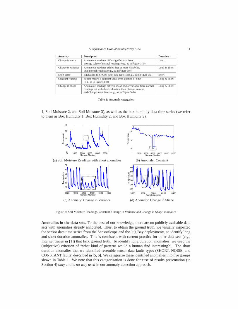
Our second sensor data source is from the Life Under Your Feetproject [13], which studiessoil ecology in a number of locations. We use data sets collected at the Jug Bay Wetland Sanctu-ary in Anne Arundel County, Maryland between June, 2007 and April, 2008. In this deployment,sensors were placed in the nests of Box Turtles to study the effect of soil temperature and soilmoisture on the incubation of turtle eggs. Measurements of soil temperature, soil moisture, boxtemperature, and box humidity are collected every 20 minutes for more than 5 months. Thesemeasurements exhibit very diverse patterns. For example, as depicted in Figure 3(a), the soilmoisture data are non-periodic – here the soil moisture readings are close to 8% when it is notraining, but they exhibit a sharp jump followed by a gradual decay when it rains. Hence, for thesoil moisture time series, instances of rainfall are the anomalies (or events) of interest that we tryto detect using SSA. In contrast, the box humidity data sets are periodic with a period of 72 datapoints (or 24 hours). The Jug Bay dataset consists of readings from 3 different sensors. In whatfollows, we show results for soil moisture readings collected (we refer to them as Soil Moisture
/ Performance Evaluation 00 (2010) 1–24 11
Anomaly Description Duration
Change in mean Anomalous readings differ significantly from Longaverage value of normal readings (e.g., as in Figure 1(a))
Change in variance Anomalous readings exhibit less or more variability Long & Shortthan normal readings (e.g., as in Figure 3(c))
Short spike Equivalent to SHORT fault data type [5] (e.g., as in Figure 3(a))Short
Constant reading Sensor reports a constant value over a period of time Long & Short(e.g., as in Figure 3(b))
Change in shape Anomalous readings differ in mean and/or variance from normal Long & Shortreadings but with shorter duration thanChange in meanandChange in variance(e.g., as in Figure 3(d))
Table 1: Anomaly categories
1, Soil Moisture 2, and Soil Moisture 3), as well as the box humidity data time series (we referto them as Box Humidity 1, Box Humidity 2, and Box Humidity 3).
0 1000 2000 3000 4000 50005
10
15
20
25
Sample Number
Per
cent
age
7950 8000 8050 8100 8150 8200
0
5
10
Sample Number
Tem
pera
ture
(a) Soil Moisture Readings with Short anomalies (b) Anomaly: Constant
3800 4000 4200 4400 4600 480010
20
30
40
50
60
70
Sample Number
Tem
pera
ture
5600 5800 6000 6200 6400
10
20
30
40
50
60
Sample Number
Tem
pera
ture
(c) Anomaly: Change in Variance (d) Anomaly: Change in Shape
Figure 3: Soil Moisture Readings, Constant, Change in Variance and Change in Shape anomalies
Anomalies in the data sets. To the best of our knowledge, there are no publicly available datasets with anomalies already annotated. Thus, to obtain the ground truth, we visually inspectedthe sensor data time series from the SensorScope and the Jug Bay deployments, to identify longand short duration anomalies. This is consistent with current practice for other data sets (e.g.,Internet traces in [1]) that lack ground truth. To identify long duration anomalies, we used the(subjective) criterion of “what kind of patterns would a human find interesting?”. The shortduration anomalies that we identified resemble sensor data faults types (SHORT, NOISE, andCONSTANT faults) described in [5, 6]. We categorize these identified anomalies into five groupsshown in Table 1. We note that this categorization is done forease of results presentation (inSection 4)onlyand isno way usedin our anomaly detection approach.
/ Performance Evaluation 00 (2010) 1–24 12
4. Experimental Results
We now evaluate our SSA-based approach and illustrate its goodness using the followingcriteria (a comparison with related literature is presented in Section 6).
• Accuracy: SSA alone detects most long duration anomalies (plus a significant fraction ofthe short duration ones), and our hybrid approach detects both, long and short durationanomalies accurately.
• Sensitivity: Our results are not sensitive to SSA’s parameter, namely tothe settings of thelinearization periodT, and the maximum linearization errorǫ.
• Cost: SSA has low computation and memory cost, and hence it can be effectively imple-mented in sensor systems.
• Robustness: SSA is robust to the presence of sensor data faults in the reference time series(i.e., there is no need to “clean” the data before running SSA).
4.1. Accuracy evaluation
We first describe our method’s accuracy, using the data sets and the ground truth identificationdescribed in Section 3. We use (1) number of false positives (detecting non-exist anomalies), and(2) number of false negatives (not being able to detect an anomaly) as our metrics. Specifically,the results in the tables below are presented as follows - thex/y number indicates thatx out of yanomalies were detected correctly (corresponding toy− x false negatives) plus we also indicatethe number of corresponding false positives (FP). Note thata long duration anomaly may consistof many consecutive data points. In this paper, we focus on detecting these events rather than onidentifying each and every anomalous data point within an event. (Thus, when 50% or more ofthe data points of a long duration anomaly are identified by SSA as anomalous, we consider thisto be a successful detection3.)
The accuracy results of our hybrid approach on all data sets are given in Tables 2 and 3. Ourhybrid method is able to detect long duration and short duration anomalies, with a small numberof false positives, and often without any false negatives. Most of the false positives are due to theRule-based part of the hybrid approach rather than to the SSApart (as explained below).
Tables 2 and 3 also show that long duration anomalies – particularly theChange in MeanandChange in Shapeanomalies – occur quite often in the SensorScope and the Jug Bay datasets(refer to the last row of both tables). For example, over the course of 43 days, a total of 84instances ofChange in Meanand 139 instancesChange in Shapeanomalies occurred in theSensorScope datasets; on average, 2 instances ofChange in Meanand 3 instances ofChange inShapeanomalies per day. Previously, others have shown that shortduration anomalies or datafaults (Short spikes, Constant readings, Noise faults) arequite prevalent in real-world datasets [5,6]; this work is the first to demonstrate that long duration anomalies occur quite often as well.
Under our hybrid approach, anomalies can be detected at three different stages – the Rule-based methods, the local step in SSA, and the aggregator stepin SSA. For both the SensorScopeand the Jug Bay datasets, we found that the aggregator step inSSA did not add significantlyto the accuracy of SSA. This is because the combination of theRule-based methods and the
3Of course, more sophisticated approaches are possible, but as our results indicate, this simple approach alreadyresults in good accuracy and allows us to focus on evaluationof SSA, without additional complications.
/ Performance Evaluation 00 (2010) 1–24 13
local step in SSA was able to detect most of the anomalies. We now focus on understandingthe contribution to our hybrid approache’s accuracy of SSA vs. the Rule-based methods. Thefirst two rows of Table 4 show the results of applying SSA alone(without the use of Rule-basedmethods) on the Soil Moisture 1 and the SensorScope 1 time series. Based on these results, wemake the following observations: (1) SSA is accurate at detecting long duration anomalies suchasChange in Average, Change in Variance, andChange in Shape, and (2) SSA can fail to detectshort duration anomalies such asShort spikes. For example, while it is able to detect more than70% of the Short spikes in Soil Moisture 1, it detects only about 50% of the Short spikes inSensorScope 1. This makes sense, as SSA is intended more for longer duration anomalies.
The utility of the hybrid approach can be seen, e.g., by comparing theShortresults for SoilMoisture 1 and SensorScope 1 in Tables 2 and 3 with those in Table 4. The hybrid approachoutperforms SSA on short duration anomalies as it uses Rule-based methods, designed specifi-cally for short duration anomalies likeShort spikesandConstant readings. However, our hybridapproach incurred a higher false positive rate than SSA, anda detailed inspection of the samplesfalsely identified as anomalous revealed that this increasewas due to the Rule-based methods.Prior work [6] showed that Rule-based methods can incur a high false positive rate mainly be-cause the histogram method for determining their fault detection threshold (Section 2.4) does notalways identify a good threshold. We also verified this by computing the histogram using theentire data set, which significantly reduced the false positive rate. However, such an approachwould not beonlineand hence not used here.
We also verified that the Rule-based methods alone do not provide any benefits in detectinglong duration anomalies. For instance, this can be seen by comparing the results for Soil Moisture1 and the SensorScope 1 data in Tables 2 and 3 with those in Table 4, where our hybrid methodperforms the same as SSA w.r.t. to detecting long duration anomalies likeChange in AverageandChange in Shape. In fact, the Rule-based methods can perform quite poorly when used foridentifying long duration anomalies. The last row of Table 4shows the results of applying theRule-based methodsaloneon the Box Humidity 2 data - compare that to the Box Humidity 2results in Table 3. As expected, the Rule-based methods detect the short duration anomalies(Shortspikes andConstantreadings), but fail to detect most of the long duration anomalies.
4.2. Sensitivity evaluation
The linearization periodT and the maximum linearization errorǫ are the two main parametersin our SSA-based approach. Next, we present an analysis of the sensitivity of our results to theseparameters’ settings.
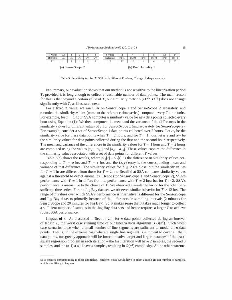
Impact of T. SSA computes the similarity measureS(D, D) everyT time units. The smallerthe value ofT, the more real-time is SSA’s anomaly detection. However, ifT is too small, theremay be too few data points for SSA to accurately capture the pattern of a long duration anomaly.Thus,T controls the trade-off between (near) real-time anomaly detection and the accuracy ofdetecting long duration anomalies.
To characterize the sensitivity of SSA’s accuracy toT, we ran SSA using different values ofT. For SensorScope datasets, we usedT values ranging from 30 minutes (the time to collect 15data points) to 8 hours (the time to collect 240 data points).For Jug Bay datasets, we variedTfrom 2 hours (the time to collect 6 data points) to 24 hours (the time to collect 72 data points).
We found that changingT’s value did not affect SSA’s accuracy w.r.t.Change in AverageandChange in Varianceanomalies, but it did affect the accuracy w.r.t.Change in Shapeanomalies.We show examples of SSA’s performance in detecting instances of theChange in Shapeanomaly

/ Performance Evaluation 00 (2010) 1–24 14
Data Set Change in Mean Change in Var Change in Shape Short Constant False PositivesSensorScope 1 3/4 0/0 6/7 90/90 2/2 7SensorScope 2 8/8 0/0 6/7 86/86 6/6 6SensorScope 3 7/7 2/2 9/10 64/64 5/5 12SensorScope 4 5/5 2/2 12/13 220/222 13/13 27SensorScope 5 6/6 4/4 9/9 726/819 34/34 0SensorScope 6 7/7 0/0 8/10 206/206 1/1 7SensorScope 7 8/8 4/4 12/12 555/567 54/54 0SensorScope 8 6/6 0/0 9/10 243/243 2/2 4SensorScope 9 6/6 2/2 11/12 65/65 23/23 6SensorScope 10 5/5 0/0 10/12 46/46 2/2 3SensorScope 11 7/7 0/0 8/10 122/122 1/1 6SensorScope 12 7/7 0/0 11/13 84/84 13/13 7SensorScope 13 8/8 2/2 13/14 250/250 15/15 5SensorScope 14 5/5 4/4 5/7 595/633 26/26 19SensorScope 15 6/6 2/2 8/9 464/475 24/24 12SensorScope 16 4/4 2/2 7/7 120/120 12/12 25SensorScope 17 5/5 4/4 6/6 166/166 17/17 13SensorScope 18 6/7 2/2 16/18 56/56 9/9 12SensorScope 19 3/3 0/0 4/6 98/98 1/1 15SensorScope 20 3/3 0/0 3/4 77/78 1/1 9SensorScope 21 2/2 1/1 3/4 332/337 26/26 5SensorScope 22 3/3 0/0 3/5 88/88 1/1 11SensorScope 23 3/3 0/0 4/4 84/84 2/2 17
Total 121/123 31/31 183/209 4837/4999 290/290 238
Table 2: Hybrid method: SensorScope
Data Set Change in Mean Change in Var Change in Shape Short Constant False PositivesSoil Moisture 1 7/8 1/1 8/10 53/55 1/1 0Soil Moisture 2 8/9 1/1 9/11 74/74 1/1 2Soil Moisture 3 5/5 0/0 6/7 42/42 0/0 4Box Humidity 1 2/2 4/4 18/19 15/15 0/0 2Box Humidity 2 5/5 7/7 27/28 16/16 2/2 2Box Humidity 3 3/3 2/2 1/1 17/17 2/2 3
Total 30/32 15/15 69/76 217/219 6/6 13
Table 3: Hybrid method: Jug Bay
in SensorScope 2 and Box Humidity 1 time series (for differentT values) in Tables 5(a) and 5(b),respectively. Very smallT values (corresponding to few data points in a linearizationperiod)result in a significant number of false positives. AsT grows, the number of false positivesimproves and becomes reasonably insensitive toT. The false negative rate is quite insensitive tothe value ofT, with a small increase for very large values ofT. Intuitively, this can be explainedas follows. For a small value ofT, SSA considers only a few data points at a time and even smalldifferences in these data points (e.g., due to measurement noise) can cause SSA to misclassifythese points as an instance ofChange in Shapeanomaly resulting in an increase in the falsepositive rate.4 The small increase in false negatives for large values ofT is due to very shortdurationChange in Shapeanomalies being “averaged out” (with a largeT).
4TheChange in Averageand theChange in Varianceanomalies occur over longer periods of time; thus, to cause a
Method Data Set Change in Mean Change in Var Change in Shape Short Constant FPSSA Soil Moisture 1 7/8 1/1 8/10 40/55 1/1 0SSA SensorScope 1 3/4 0/0 6/7 46/90 1/2 1
Rule based Box Humidity 2 2/5 0/7 5/28 16/16 2/2 2
Table 4: SSA vs. Rule-based methods
/ Performance Evaluation 00 (2010) 1–24 15
T Value 0.5 1 2 4 8Detected 7/7 7/7 6/7 6/7 6/7
FP 8 4 0 0 0
T Value 2 4 6 8 12 24Detected 19/19 19/19 19/19 19/19 18/19 18/19
FP 17 10 6 4 2 2
(a) SensorScope 2 (b) Box Humidity 1
Table 5: Sensitivity test forT: SSA with differentT values; Change of shape anomaly
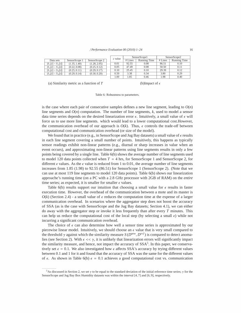
In summary, our evaluation shows that our method is not sensitive to the linearization periodT, provided it is long enough to collect a reasonable number ofdata points. The main reasonfor this is that beyond a certain value ofT, our similarity metricS(Dnew,Dre f ) does not changesignificantly withT, as illustrated next.
For a fixedT value, we ran SSA on SensorScope 1 and SensorScope 2 separately, andrecorded the similarity values (w.r.t. to the reference time series) computed everyT time units.For example, forT = 1 hour, SSA computes a similarity value for new data points collected everyhour using Equation (1). We then computed the mean and the variance of the differences in thesimilarity values for different values ofT for SensorScope 1 (and separately for SensorScope 2).For example, consider a set of SensorScope 1 data points collected over 2 hours. Letα2 be thesimilarity value for these data points whenT = 2 hours, and forT = 1 hour, letα11 andα12 bethe similarity values for data points collected during the first and the second hour, respectively.The mean and variance of the differences in the similarity values forT = 1 hour andT = 2 hoursare computed using the values|α2 − α11| and |α2 − α12|. These values capture the difference inthe similarity values associated with a set of data points for differentT values.
Table 6(a) shows the results, where|Sq[t] − Sr [t]| is the difference in similarity values cor-responding toT = q hrs andT = r hrs and the (x, y) entry is the corresponding mean andvariance of that difference. The similarity values forT ≥ 2 are close, but the similarity valuesfor T = 1 hr are different from those forT = 2 hrs. Recall that SSA compares similarity valuesagainst a threshold to detect anomalies. Hence (for SensorScope 1 and SensorScope 2), SSA’sperformance withT = 1 hr differs from its performance withT = 2 hrs; but forT ≥ 2, SSA’sperformance is insensitive to the choice ofT. We observed a similar behavior for the other Sen-sorScope time series. For the Jug Bay dataset, we observed similar behavior forT ≥ 12 hrs. Therange ofT values over which SSA’s performance is insensitive is different for the SensorScopeand Jug Bay datasets primarily because of the differences in sampling intervals (2 minutes forSensorScope and 20 minutes for Jug Bay). So, it makes sense that it takes much longer to collecta sufficient number of samples in the Jug Bay data sets and hence requires a largerT to achieverobust SSA performance.
Impact of ǫ. As discussed in Section 2.4, forn data points collected during an intervalof lengthT, the worst case running time of our linearization algorithmis O(n2). Such worstcase scenarios arise when a small number of line segments aresufficient to model alln datapoints. That is, in the extreme case where a single line segment is sufficient to cover all thendata points, our greedy approach will be forced to solve larger and larger instances of the least-square regression problem in each iteration – the first iteration will have 2 samples, the second 3samples, and the (n-1)st will haven samples, resulting inO(n2) complexity. At the other extreme,
false positive corresponding to these anomalies, (random) noise would have to affect a much greater number of samples,which is unlikely to happen.
/ Performance Evaluation 00 (2010) 1–24 16
Data sets SensorScope 1 SensorScope 2|S1[t] − S2[t]| (1.35, 1.40) (1.28, 2.05)|S2[t] − S3[t]| (0.22, 0.08) (0.25, 0.12)|S3[t] − S4[t]| (0.25, 0.11) (0.29, 0.17)|S4[t] − S6[t]| (0.29, 0.14) (0.30, 0.20)
ǫ valueSensorScope1 SensorScope2
# Lines Running Time # Lines Running Time0.01 92.55 0.08 86.51 0.100.05 47.49 0.08 50.50 0.110.10 25.45 0.10 29.39 0.120.50 3.38 0.34 3.80 0.291.00 1.85 0.46 1.98 0.40
(a) Similarity metric as a function ofT (b)Impact ofǫ
Table 6: Robustness to parameters.
is the case where each pair of consecutive samples defines a new line segment, leading toO(n)line segments andO(n) computation. The number of line segments,k, used to model a sensordata time series depends on the desired linearization errorǫ. Intuitively, a small value ofǫ willforce us to use more line segments. which would lead to a lowercomputational cost.However,the communication overhead of our approach isO(k). Thus,ǫ controls the trade-off betweencomputational cost and communication overhead (or size of the model).
We found that in practice (e.g., in SensorScope and Jug Bay datasets) a small value ofǫ resultsin each line segment covering a small number of points. Intuitively, this happens as typicallysensor readings exhibit non-linear patterns (e.g., diurnal or sharp increases in value when anevent occurs), and approximating non-linear patterns using line segments results in only a fewpoints being covered by a single line. Table 6(b) shows the average number of line segments usedto model 120 data points collected whenT = 4 hrs, for SensorScope 1 and SensorScope 2, fordifferentǫ values. As theǫ value is reduced from 1 to 0.01, the average number of line segmentsincreases from 1.85 (1.98) to 92.55 (86.51) for SensorScope 1 (SensorScope 2). (Note that wecan use at most 119 line segments to model 120 data points). Table 6(b) shows our linearizationapproache’s running time (on a PC with a 2.8 GHz processor with 2GB of RAM) on theentiretime series; as expected, it is smaller for smallerǫ values.
Table 6(b) results support our intuition that choosing a small value for ǫ results in fasterexecution time. However, the overhead of the communicationbetween a mote and its master isO(k) (Section 2.4) - a small value ofǫ reduces the computation time at the expense of a largercommunication overhead. In scenarios where the aggregatorstep does not boost the accuracyof SSA (as is the case with SensorScope and the Jug Bay datasets; Section 4.1), we can eitherdo away with the aggregator step or invoke it less frequentlythan after everyT minutes. Thiscan help us reduce the computational cost of the local step (by selecting a smallǫ) while notincurring a significant communication overhead.
The choice ofǫ can also determine how well a sensor time series is approximated by ourpiecewise linear model. Intuitively, we should choose anǫ value that is very small compared tothe thresholdγ against which the similarity measureS(Dnew,Dre f ) is compared to detect anoma-lies (see Section 2). Withǫ << γ, it is unlikely that linearization errors will significantly impactthe similarity measure, and hence, not impact the accuracy of SSA5. In this paper, we conserva-tively setǫ = 0.1. We also investigated howǫ affects SSA’s accuracy by trying different valuesbetween 0.1 and 1 for it and found that the accuracy of SSA was the same forthe different valuesof ǫ. As shown in Table 6(b)ǫ = 0.1 achieves a good computational cost vs. communication
5As discussed in Section 2, we setγ to be equal to the standard deviation of the initial reference time series;γ for theSensorScope and Jug Bay Box Humidity datasets was within the interval [4,7] and [6,9], respectively.
/ Performance Evaluation 00 (2010) 1–24 17
overhead trade-off – choosing a smaller value did not reduce the running time significantly butled to a large increase in the number of line segmentsk.
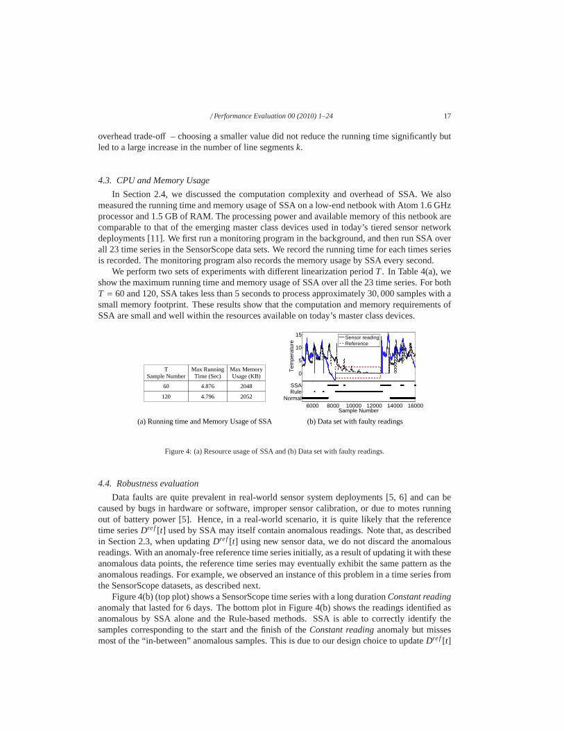
4.3. CPU and Memory Usage
In Section 2.4, we discussed the computation complexity andoverhead of SSA. We alsomeasured the running time and memory usage of SSA on a low-endnetbook with Atom 1.6 GHzprocessor and 1.5 GB of RAM. The processing power and available memory of this netbook arecomparable to that of the emerging master class devices usedin today’s tiered sensor networkdeployments [11]. We first run a monitoring program in the background, and then run SSA overall 23 time series in the SensorScope data sets. We record therunning time for each times seriesis recorded. The monitoring program also records the memoryusage by SSA every second.
We perform two sets of experiments with different linearization periodT. In Table 4(a), weshow the maximum running time and memory usage of SSA over allthe 23 time series. For bothT = 60 and 120, SSA takes less than 5 seconds to process approximately 30,000 samples with asmall memory footprint. These results show that the computation and memory requirements ofSSA are small and well within the resources available on today’s master class devices.
0.6 0.8 1 1.2 1.4x 10
4
0
5
10
15
Tem
pera
ture
6000 8000 10000 12000 14000 16000Normal
RuleSSA
Sample Number
Sensor readingReference
(b) Data set with faulty readings(a) Running time and Memory Usage of SSA
TSample Number
Max RunningTime (Sec)
Max MemoryUsage (KB)
60 4.876 2048
120 4.796 2052
Figure 4: (a) Resource usage of SSA and (b) Data set with faulty readings.
4.4. Robustness evaluation
Data faults are quite prevalent in real-world sensor systemdeployments [5, 6] and can becaused by bugs in hardware or software, improper sensor calibration, or due to motes runningout of battery power [5]. Hence, in a real-world scenario, itis quite likely that the referencetime seriesDre f [t] used by SSA may itself contain anomalous readings. Note that, as describedin Section 2.3, when updatingDre f [t] using new sensor data, we do not discard the anomalousreadings. With an anomaly-free reference time series initially, as a result of updating it with theseanomalous data points, the reference time series may eventually exhibit the same pattern as theanomalous readings. For example, we observed an instance ofthis problem in a time series fromthe SensorScope datasets, as described next.
Figure 4(b) (top plot) shows a SensorScope time series with along durationConstant readinganomaly that lasted for 6 days. The bottom plot in Figure 4(b)shows the readings identified asanomalous by SSA alone and the Rule-based methods. SSA is able to correctly identify thesamples corresponding to the start and the finish of theConstant readinganomaly but missesmost of the “in-between” anomalous samples. This is due to our design choice to updateDre f [t]
/ Performance Evaluation 00 (2010) 1–24 18
using anomalous samples as well. We can see in Figure 4(b) (top plot) that after (approximately)400 successive samples corrupted by theConstant readinganomaly, the reference time seriesvalues are quite close to the anomalous readings, and as a result, SSA does not stops flagging thesubsequent readings as anomalous. In Section 2, we justifiedour use of anomalous readings toupdateDre f [t] by demonstrating that it helps us “zoom in” on samples wherethe sharp changesin sensor readings happen (see Figure 2(a)). However, as this example shows, updatingDre f [t]using anomalous readings can cause SSA to miss a large numberof samples affected by a longduration anomaly, and only identify the beginning and end ofa long duration anomalous event.This again motivates the use of our hybrid approach - i.e., for the time series in Figure 4(b)(bottom plot), we identify the samples missed by SSA using the CONSTANT rule.
The SensorScope time series in Figure 4(b) (top plot) also contains two instances ofShortspikes(that occur before the long durationConstantanomaly). Even though SSA alone fails todetect them, their presence does not impair SSA’s ability todetect the long duration anomalythat occurs later. Hence, we do not need to “clean” the time series data before running SSA. Wecan see in Figure 4(b) (top plot) that the SHORT faults do not affect the reference time seriessignificantly, i.e., SSA is robust to faults.
5. Related Work
Anomaly detection is an area of active research. In this section we briefly survey work mostrelated to ours, organized into four categories. Moreover,we select representative techniquesfrom these categories and quantitatively compare them against our hybrid approach, with resultsof this comparison presented in Section 6.
Anomaly detection in sensor systems. This is not a well-studied area. The only efforts we areaware of that focus on anomaly detection in sensor systems data are [7, 8, 9]. Rajasegarar et al.[7] present a clustering based method based onK nearest neighbor algorithm in [7], and a SVMbased approach in [8]. Briefly, these works view measurements collected by a sensor systemas coming from the same (unknown) distribution and “pre-define” anomalies as outliers, withmain focus of these (offline) techniques being on minimizing the communication overhead (intransmitting data needed for anomaly detection) and the corresponding energy consumption. Incontrast, we focus on anonlineapproach, without “pre-defining” what is an anomaly. However,we do perform a quantitative comparison between our hybrid approach and the clustering basedmethod in [7]. The details of this comparison can be found in Section 6.
Tartakovsky et al. use a change point detection based approach, CUSUM (Cumulative SumControl Chart), for quickly detecting distribution changes (e.g., mean, variance, covariances) insensor measurements [9]. We do not provide a quantitative comparison between CUSUM andour hybrid approach as we lack sufficient domain knowledge - i.e., the CUSUM based approachassumes knowledge of the (time varying) probability distribution from which sensor measure-ments are sampled, and such information is not provided for the SensorScope and the Jug Baydatasets (and would be quite difficult for us to compute accurately).
In general, change point detection can identify changes in the parameters of a stochasticprocess. Often, such changes are anomalous, and hence, change point detection techniques havebeen used for change/outlier detection in time series data [15, 16]. However, such existing works(a) assume that sensor measurements are sampled from a knownor easily inferred distribution(e.g., Gaussian), an assumption often not true for real world datasets, (b) target a specific subsetof anomalies, and (c) do not use real-world sensor datasets for evaluation. In addition, existing

/ Performance Evaluation 00 (2010) 1–24 19
change point detection based methods either require a long training phase, or are computationallyintensive, or (in some cases) both – hence, they do not meet our efficiency criteria. Moreover,not all changes in a time series might be anomalous, i.e., there could be a change and no anomaly(i.e., a false positive) and vice versa (i.e., a false negative). For example, [15] flags turning pointsof a time series from increasing to decreasing – as it is often“normal” for a sensor data timeseries to have periodic behavior, this is (likely) not an anomaly. On the other hand, such anapproach would only flag a few turning points, instead of an entire anomalous event, as depictedin Figure 1(a). We believe that change point detection couldbe a promising approach to anomalydetection, but that it would require significant work to devise an accurate and efficient onlineanomaly detection method based on such techniques.
Fault detection in sensor systems. Short duration anomalies can be viewed as instances of datafaults, errors in measurements, or outliers (see [5]). Sharma et al. focus on SHORT spikes,NOISE faults, and CONSTANT readings data faults and show that these are quite prevalent inreal-world sensor datasets [6]. They also evaluate the performance of several methods – Rule-based methods, a least-squares estimation based method, Hidden Markov model (HMM) basedmethod, and a time series analysis (ARIMA model) based method–that are targeted towardsdetecting transient sensor data faults. However, these methods perform poorly at detecting longduration anomalies. E.g., in Section 4.1 we showed that Rule-based methods are not sufficient fordetecting long duration anomalies. Other than that, we alsocompare the ARIMA model basedapproach, which works best in case of data faults affecting more than a few samples, against ourhybrid approach (with details given in Section 6).
Other approaches to sensor data faults detection include [17, 18, 19, 20]. However, these arenot suited for detecting (unknown) long duration anomaliesdue to one or more of the followingassumptions they make: (1) the anomalous data pattern is known a priori [17, 18, 19], (2) thedistribution of normal sensor readings is known [19], and (3) focusing on short duration trendsis enough to capture anomalies [20].
Network anomaly detection. The work in this area includes detecting anomalies such as DDoSattacks, flash crowds, worm propagating, bulk data transferin enterprise or ISP networks [1, 2,3, 4]. Techniques such as Principal Component Analysis (PCA) [1] and wavelet analysis [2,3, 4], used for detecting network traffic anomalies, are not well suited foronline detection insensor systems primarily because they are computationallyintensive and difficult to perform inan online manner. Furthermore, we show that even in an offline manner, these methods performpoorly in detecting long duration anomaly on sensor system data (as detailed in Section 6).Our quantitative study (given in Section 6) indicates that astraightforward application of suchtechniques, as designed for network anomaly detection, is not very effective on sensor data.
Piecewise linear time series models. Piecewise linear models have been used to model timeseries data in the other contexts (i.e., not for anomaly detection). For example, Keogh developedan efficient technique to search for occurrences of aknown patternwithin a time series usinga piecewise linear representation [10]. Specifically, for atime series withn points, Keogh’salgorithm starts withk = ⌊ n3⌋ line segments and defines a “goodness of fit” metric fork linesegments asBk=std(e1, ...,ek), whereei is the average linearization error for line segmenti. Itthen iteratively merges two consecutive line segments until Bk cannot be reduced any further;this process is continued until a single line approximates the entire time series. This processends with a family of piecewise linear models for a single time series – one for each value ofk,1 ≤ k ≤ ⌊ n3⌋. Each linear model has aBk value associated with it, and the one with the smallest

/ Performance Evaluation 00 (2010) 1–24 20
Bk is selected as the final representation.In contrast, our greedy linearization algorithm differs as follows: (1) we start with a single
line segment and continue adding more segments, (2) we use a different “goodness of fit” cri-terion (maximum linearization error; see Section 2) and (3)we compute a single representationinstead of a family of piecewise linear models. The main reason behind these choices (ratherthan, e.g., using Keogh’s algorithm) is computational costas our goal is an efficientonlineap-proach. Briefly, computing a family of models to find the “best” one is wasteful for our purposes,if it takes significantly greater computation. Hence, we optfor our greedy approach.
6. Quantitative comparison
We now present results from a quantitative comparison of ourhybrid approach and anomalydetection techniques based on ARIMA models [6], PCA [1], wavelets decomposition [3], and K-means clustering [7]. As noted above, these techniques haveproven to be effective at detectingsensor data faults and network anomalies. However, our evaluation shows that an “out-of-a-box”application of these techniques for detecting sensor system anomalies performs poorly.
Comparison with ARIMA based method. ARIMA (Autoregressive Integrated Moving Av-erage) models are a standard tool for modeling and forecasting time series data with periodic-ity [21], and [6] leverages temporal correlations in sensormeasurements to construct an ARIMAmodel of sensor data. This model is used to predict the value of future readings, with new sen-sor readings compared against their predicted value - if thedifference between these values isabove a threshold (the 95% confidence interval for the predictions) then the new data is markedas anomalous. We compare our hybrid approach against the ARIMA L-step method from [6],where the ARIMA model is used to predict the nextL sensor readings.
We first trained the ARIMA model to estimate its parameters using sensor readings (fromSensorScope 1 and SensorScope 2) collected over 3 days as training data (a separate trainingphase was required for SensorScope 1 and SensorScope 2, [6] also uses training data from 3 days;these are more favorable conditions for ARIMA as SSA uses a shorter period for its referencemodel). The ARIMA L-step method withL = 24 hrs flagged 12,135 (of the 30,356 data points inSensorScope 1) as anomalies. Our inspection revealed a total of 107 anomalies that affect morethan 7,500 data points. While the ARIMA L-step method identified most anomalous samples, italso falsely identified a large number of samples as anomalous. The extremely high number offalse positives resulting from the ARIMA L-step method reduces its utility.
We failed to train ARIMA on SensorScope 2 due to the training data containing aConstantreadingsanomaly that affects almost two-thirds of the samples. This failure highlights the lackof robustness in ARIMA based methods to long duration anomalies in the training data. SSA’scounterpart to the ARIMA training phase is the selection of an initial reference time series, andSSA tolerates anomalies in its initial reference time series (see Section 4.4).
Comparison with network anomaly detection techniques. The techniques such as PrincipalComponent Analysis (PCA) [1], and wavelet analysis [3, 2, 4]used for detecting network trafficanomalies are not well suited foronlinedetection in sensor systems primarily because they arecomputationally intensive and difficult to perform in an online manner. However, one can stillask: How accurately would those technique perform on sensor systems data?, i.e., in an offlinemanner. As a reasonably representative technique, we use the PCA based approach in [1], whichcollects periodic measurements of the traffic on all network links and splits it into “normal”
/ Performance Evaluation 00 (2010) 1–24 21
and “residual” traffic using PCA. The residual traffic is then mined for anomalies using the Q-statistic test in which L2-norm||y||2 of the residual traffic vectory for a link is compared againsta threshold. If it is greater than the threshold, then the traffic vectory is declared anomalous [1].
We ran the PCA based method on the data from SensorScope time series 6, 8, 9, 10, 11, and12. We chose these as their start and end times are the same. The input to PCA was a data matrixwith 6 columns (one for each sensor) and 29,518 rows (the total number of samples collected).Note that the PCA based method is applied in anoffline fashion using the entire time series datafrom 6 different sensors whereas in our SSA-based hybrid approach, at best, the aggregator stepwould get access to linear models from 6 sensors during the past T = 4 hours only.
The results for the PCA based method are summarized in Table 7. It fails to detect mostlong duration anomalies (5 out of 38Change in Meananomalies and 4 out of 67Change inShapeanomalies). It does better at detectingShort spikesbut is still not as accurate as our hybridapproach. Thus, even under a best case scenario (offline with access to the entire time series),the PCA based method does not perform as well as our hybrid approach. Recall that it identifiesanomalies by looking at the L2-norm of the data vector in the residual space. As pointed out in[1], the PCA based method works best when theintensityof an anomaly is large compared tothe variability of the normal data. This is not the case with most of the long duration anomaliespresent in the sensor data analyzed in Table 7. For instance,Figure 5(a) shows aChange in Meananomaly in SensorScope 12 time series that the PCA based method fails to detect. It also showsaShortanomaly (spike) that the PCA based method is able to detect.
To further illustrate the impact of anomalies’ intensitieson the accuracy of a PCA-basedmethod, we injected anomalies (Short, Noise, and Constant)into the time series SensorScope 9,and attempted to detect these injected faults using PCA. Thedata samples corrupted by Short andNoise anomalies had a higher variance as compared to the normal data whereas, by definition, thevariance of the samples corrupted by the Constant anomaly was lower than the normal data. Wefound that the PCA based method was able to detect most of the samples corrupted by SHORTand NOISE anomalies, but missed the Constant anomaly. We do not present these here due tolack of space; these results can be found in our technical report [22].
Apart from the intensity of an anomaly, the PCA results mightalso be impacted by severalother factors such as sensitivity of PCA to its parameters and lack of data preprocessing. Forinstance, [23] shows that the performance of PCA is sensitive to the number of principal compo-nents included in the normal subspace, and the threshold used for anomaly detection. We notethat, in our experiments, we did vary the number of principalcomponents in the normal subspace,and Table 7 depicts the best results obtained (i.e., those with having only 1 principal componentin the normal space). To our knowledge, the Q-statistic based technique that we use here is theonly known method for automatically deciding the detectionthreshold. It is also well-knownthat anomalies can contaminate the normal subspace and hence, avoid detection by PCA [23].One way to ameliorate this situation can be to preprocess thedata to identify and remove largeanomalies before applying PCA. However, in our context, defining alarge anomaly would itselfhave required us to introduce another heuristic (with its own shortcomings). We do not pursuethis (or other PCA related improvements) further, as the main goal of our PCA-based evaluationhere was to illustrate that, as in the case of network anomalydetection, it is not straightforwardto apply PCA to detect anomalies in sensor data. (This partlycontributed to our choice of a dif-ferent approach.) Of course, we do not claim that the PCA based method cannot be made moreeffective at detecting sensor data anomalies, but as noted, this is not the goal of our work here.
To the same end, we also explore wavelet based methods for detecting sensor data anomalies.We select the method presented in [3] as a representative technique. This method first separates
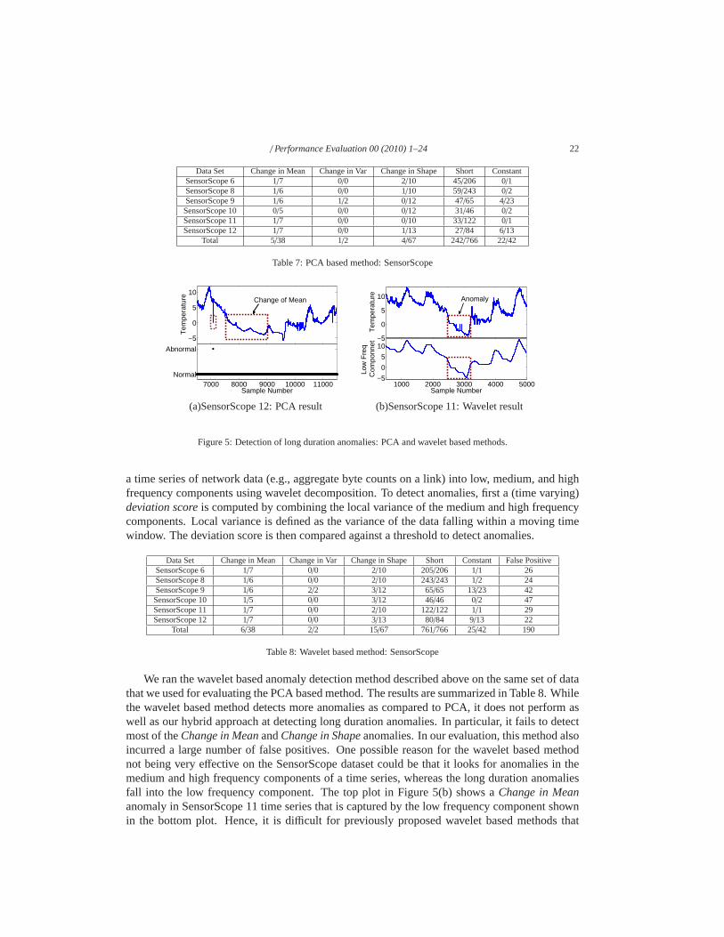
/ Performance Evaluation 00 (2010) 1–24 22
Data Set Change in Mean Change in Var Change in Shape Short ConstantSensorScope 6 1/7 0/0 2/10 45/206 0/1SensorScope 8 1/6 0/0 1/10 59/243 0/2SensorScope 9 1/6 1/2 0/12 47/65 4/23SensorScope 10 0/5 0/0 0/12 31/46 0/2SensorScope 11 1/7 0/0 0/10 33/122 0/1SensorScope 12 1/7 0/0 1/13 27/84 6/13
Total 5/38 1/2 4/67 242/766 22/42
Table 7: PCA based method: SensorScope
7000 8000 9000 10000 11000−5
0
5
10
Tem
pera
ture
7000 8000 9000 10000 11000Normal
Abnormal
Sample Number
Change of Mean
10001500200025003000350040004500−5
0
5
10
Tem
pera
ture
1000 2000 3000 4000 5000−5
0
5
10
Sample Number
Low
Fre
q C
ompo
nnet
Anomaly
(a)SensorScope 12: PCA result (b)SensorScope 11: Wavelet result
Figure 5: Detection of long duration anomalies: PCA and wavelet based methods.
a time series of network data (e.g., aggregate byte counts ona link) into low, medium, and highfrequency components using wavelet decomposition. To detect anomalies, first a (time varying)deviation scoreis computed by combining the local variance of the medium andhigh frequencycomponents. Local variance is defined as the variance of the data falling within a moving timewindow. The deviation score is then compared against a threshold to detect anomalies.
Data Set Change in Mean Change in Var Change in Shape Short Constant False PositiveSensorScope 6 1/7 0/0 2/10 205/206 1/1 26SensorScope 8 1/6 0/0 2/10 243/243 1/2 24SensorScope 9 1/6 2/2 3/12 65/65 13/23 42SensorScope 10 1/5 0/0 3/12 46/46 0/2 47SensorScope 11 1/7 0/0 2/10 122/122 1/1 29SensorScope 12 1/7 0/0 3/13 80/84 9/13 22
Total 6/38 2/2 15/67 761/766 25/42 190
Table 8: Wavelet based method: SensorScope
We ran the wavelet based anomaly detection method describedabove on the same set of datathat we used for evaluating the PCA based method. The resultsare summarized in Table 8. Whilethe wavelet based method detects more anomalies as comparedto PCA, it does not perform aswell as our hybrid approach at detecting long duration anomalies. In particular, it fails to detectmost of theChange in MeanandChange in Shapeanomalies. In our evaluation, this method alsoincurred a large number of false positives. One possible reason for the wavelet based methodnot being very effective on the SensorScope dataset could be that it looks for anomalies in themedium and high frequency components of a time series, whereas the long duration anomaliesfall into the low frequency component. The top plot in Figure5(b) shows aChange in Meananomaly in SensorScope 11 time series that is captured by thelow frequency component shownin the bottom plot. Hence, it is difficult for previously proposed wavelet based methods that
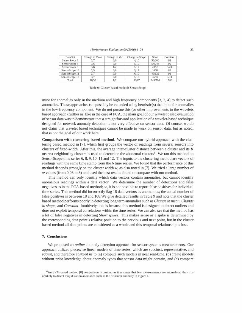
/ Performance Evaluation 00 (2010) 1–24 23
Data Set Change in Mean Change in Var Change in Shape Short ConstantSensorScope 6 2/7 0/0 4/10 56/206 1/1SensorScope 8 3/6 0/0 5/10 54/243 1/2SensorScope 9 3/6 1/2 5/12 20/65 5/23SensorScope 10 2/5 0/0 5/12 16/46 1/2SensorScope 11 3/7 0/0 6/10 49/122 1/1SensorScope 12 3/7 0/0 5/13 36/84 3/13
Total 16/38 1/2 30/67 243/766 12/42
Table 9: Cluster based method: SensorScope
mine for anomalies only in the medium and high frequency components [3, 2, 4] to detect suchanomalies. These approaches can possibly be extended usingheuristic(s) that mine for anomaliesin the low frequency component. We do not pursue this (or other improvements to the waveletsbased approach) further as, like in the case of PCA, the main goal of our wavelet based evaluationof sensor data was to demonstrate that a straightforward application of a wavelet-based techniquedesigned for network anomaly detection is not very effective on sensor data. Of course, we donot claim that wavelet based techniques cannot be made to work on sensor data, but as noted,that is not the goal of our work here.
Comparison with clustering based method. We compare our hybrid approach with the clus-tering based method in [7], which first groups the vector of readings from several sensors intoclusters of fixed-width. After this, the average inter-cluster distance between a cluster and itsKnearest neighboring clusters is used to determine the abnormal clusters6. We ran this method onSensorScope time series 6, 8, 9, 10, 11 and 12. The inputs to the clustering method are vectors ofreadings with the same time stamp from the 6 time series. We found that the performance of thismethod depends strongly on the cluster widthw, as also noted in [7]. We tried a large number ofw values (from 0.03 to 8) and used the best results found to compare with our method.
This method can only identify which data vectors contain anomalies, but cannot identifyanomalous readings within a data vector. We determine the number of detections and falsenegatives as in the PCA-based method; so, it is not possible to report false positives for individualtime series. This method did incorrectly flag 18 data vectorsas anomalous; the actual number offalse positives is between 18 and 108.We give detailed results in Table 9 and note that the clusterbased method performs poorly in detecting long term anomalies such asChange in mean, Changein shape, andConstant. Intuitively, this is because this method is designed to detect outliers anddoes not exploit temporal correlations within the time series. We can also see that the method hasa lot of false negatives in detectingShort spikes. This makes sense as a spike is determined bythe corresponding data point’s relative position to the previous and next point, but in the clusterbased method all data points are considered as a whole and this temporal relationship is lost.
7. Conclusions
We proposed anonlineanomaly detection approach for sensor systems measurements. Ourapproach utilized piecewise linear models of time series, which are succinct, representative, androbust, and therefore enabled us to (a) compute such models in near real-time, (b) create modelswithout prior knowledge about anomaly types that sensor data might contain, and (c) compare
6An SVM-based method [8] comparison is omitted as it assumes that few measurements are anomalous; thus it isunlikely to detect long duration anomalies such as theConstantanomaly in Figure 4.
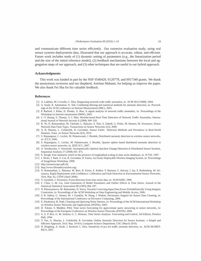
/ Performance Evaluation 00 (2010) 1–24 24
and communicate different time series efficiently. Our extensive evaluation study, using realsensor systems deployments data, illustrated that our approach is accurate, robust, and efficient.Future work includes study of (1) dynamic setting of parameters (e.g., the linearization periodand the size of the initial reference model), (2) feedback mechanisms between the local and ag-gregation steps of our approach, and (3) other techniques that are useful in our hybrid approach.
Acknowledgments
This work was funded in part by the NSF 0540420, 0120778, and 0917340 grants. We thankthe anonymous reviewers and our shepherd, Anirban Mahanti,for helping us improve the paper.We also thank Fei Sha for his valuable feedback.
References
[1] A. Lakhina, M. Crovella, C. Diot, Diagnosing network-wide traffic anomalies, in: ACM SIGCOMM, 2004.[2] A. Soule, K. Salamatian, N. Taft, Combining filtering and statistical methods for anomaly detection, in: Proceed-
ings of the ACM conference on Internet Measurement (IMC), 2005.[3] P. Barford, J. Kline, D. Plonka, A. Ron, A signal analysisof network traffic anomalies, in: Proceedings of the
Workshop on Internet measurment (IMW), 2002.[4] C.-T. Huang, S. Thareja, Y.-J. Shin, Wavelet-based RealTime Detection of Network Traffic Anomalies, Interna-
tional Journal of Network Security 6 (2008) 309–320.[5] K. Ni, N. Ramanathan, M. Chehade, L. Balzano, S. Nair, S. Zahedi, G. Pottie, M. Hansen, M. Srivastava, Sensor
Network Data Fault Types, Transactions on Sensor Networks 5(3), 2009.[6] A. B. Sharma, L. Golubchik, R. Govindan, Sensor Faults: Detection Methods and Prevalence in Real-World
Datasets, Trans. on Sensor Networks 6(3), 2010.[7] S. Rajasegarar, C. Leckie, M. Palaniswami, J. Bezdek, Distributed anomaly detection in wireless sensor networks,
in: ICCS, 2006.[8] S. Rajasegarar, C. Leckie, M. Palaniswami, J. Bezdek, Quarter sphere based distributed anomaly detection in
wireless sensor networks, in: IEEE ICC, 2007.[9] A. Tartakovsky, V. Veeravalli, Asymptotically Optimal Quickest Change Detection in Distributed Sensor Systems,
Sequential Analysis 27 (2008) 441–475.[10] E. Keogh, Fast similarity search in the presence of longitudinal scaling in time series databases, in: ICTAI, 1997.[11] J. Hicks, J. Paek, S. Coe, R. Govindan, D. Estrin, An Easily Deployable Wireless Imaging System, in: Proceedings
of ImageSense Workshop, 2008.[12] http://sensorscope.epfl.ch/.[13] http://www.lifeunderyourfeet.org/.[14] N. Ramanathan, L. Balzano, M. Burt, D. Estrin, E. Kohler,T. Harmon, C. Harvey, J. Jay, S. Rothenberg, M. Sri-
vastava, Rapid Deployment with Confidence: Calibration and Fault Detection in Environmental Sensor Networks,Tech. Rep. 62, CENS (April 2006).
[15] V. Guralnik, J. Srivastava, Event detection from time series data, in: ACM KDD, 1999.[16] C. Chen, L.-M. Liu, Joint Estimation of Model Parameters and Outlier Effects in Time Series, Journal of the
American Statistical Association 88 (1993) 284–297.[17] N. Khoussainova, M. Balazinska, D. Suciu, Towards Correcting Input Data Errors Probabilistically Using Integrity
Constraints, in: Proceedings of the ACM Workshop on Data Engineering and Mobile Access, 2006.[18] S. R. Jeffery, G. Alonso, M. J. Franklin, W. Hong, J. Widom, DeclarativeSupport for Sensor Data Cleaning, in:
Proceedings of the International Conference on Pervasive Computing, 2006.[19] E. Elnahrawy, B. Nath, Cleaning and Querying Noisy Sensors, in: Proceedings of the ACM International Workshop
on Wireless Sensor Networks and Applications (WSNA), 2003.[20] D. Tulone, S. Madden, PAQ: Time series forecasting for approximate query answering in sensor networks, in:
Proceedings of the European Conference on Wireless Sensor Networks (EWSN), 2006.[21] G. E. P. Box, G. M. Jenkins, G. C. Reinsen, Time Series Analysis: Forecasting and Control, 3rd Edition, Prentice
Hall, 1994.[22] Y. Yao, A. Sharma, L. Golubchik, R. Govindan, Online Anomaly Detection for Sensor Systems: a Simple and
Efficient Approach, Tech. Rep. 10-914, Computer Science Department, USC (March 2010).[23] H. Ringberg, A. Soule, J. Rexford, C. Diot, Sensitivityof pca for traffic anomaly detection, in: ACM SIGMET-
RICS, 2007.


![Embedded Intelligence: Sensor Networks and Beyond · Structural monitoring [Pakzad et al., 2005] • Detecting changes in the environment: – Thresholds, phase transitions, anomaly](https://img.pdfslide.net/doc/110x75/5ed28055ad716a665e6d9269/embedded-intelligence-sensor-networks-and-beyond-structural-monitoring-pakzad.jpg)