Embed Size (px)
Citation preview
J. Grid Computing
DOI 10.1007/s10723-015-9340-0
Online Bi-Objective Scheduling for IaaS Clouds Ensuring
Quality of Service
Andrei Tchernykh Luz Lozano Uwe Schwiegelshohn
Pascal Bouvry Johnatan E. Pecero
Sergio Nesmachnow Alexander Yu. Drozdov
Received: November 2014 / Accepted 4 July 2015:
© Springer Science+Business Media B.V. 2015
Abstract. This paper focuses on a bi-objective experimental
evaluation of online scheduling in the Infrastructure as a
Service model of Cloud computing regarding income and
power consumption objectives. In this model, customers
have the choice between different service levels. Each
service level is associated with a price per unit of job
execution time, and a slack factor that determines the
maximal time span to deliver the requested amount of
computing resources. The system, via the scheduling
algorithms, is responsible to guarantee the corresponding
quality of service for all accepted jobs. Since we do not
consider any optimistic scheduling approach, a job cannot
be accepted if its service guarantee will not be observed
assuming that all accepted jobs receive the requested
resources. In this article, we analyze several scheduling
algorithms with different cloud configurations and
workloads, considering the maximization of the provider
income and minimization of the total power consumption of
a schedule. We distinguish algorithms depending on the type
and amount of information they require: knowledge free,
energy-aware, and speed-aware. First, to provide effective
guidance in choosing a good strategy, we present a joint
analysis of two conflicting goals based on the degradation in
performance. The study addresses the behavior of each
strategy under each metric. We assess the performance of
different scheduling algorithms by determining a set of non-
dominated solutions that approximate the Pareto optimal set.
We use a set coverage metric to compare the scheduling
algorithms in terms of Pareto dominance.
Andrei Tchernykh ∙ Luz Lozano
CICESE Research Center, Ensenada, Baja California, México, {chernykh,
llozano}@cicese.mx
Uwe Schwiegelshohn
TU Dortmund University, Dortmund, Germany,
Pascal Bouvry ∙ Johnatan E. Pecero
University of Luxembourg, Luxembourg,
{Pascal.Bouvry, Johnatan.Pecero}@uni.lu
Sergio Nesmachnow
Universidad de la República, Uruguay, [email protected]
Alexander Yu. Drozdov
Moscow Institute of Physics and Technology,
We claim that a rather simple scheduling approach can
provide the best energy and income trade-offs. This
scheduling algorithm performs well in different scenarios
with a variety of workloads and cloud configurations.
Keywords Cloud computing Service Level Agreement
Energy Efficiency Multi-objective Scheduling IaaS
1 Introduction
The implementation of a service-oriented paradigm in
computing leads to Service Level Agreements (SLAs). The
concurrent availability of different service levels in multi-
user systems must have a strong influence on job scheduling
since customers with better service levels expect preferred
attendance. To be attractive to a wide range of customers
providers want to accommodate different needs that are
different levels of service.
As a representative of present IaaS providers, we use
Amazon Web Services (AWS). An AWS-customer can
select one of several instances that differ in virtual CPUs,
RAM, and memory. In addition, the customer can add
additional services like network, data bases, and applications.
If a provider is running out a requested instance, he may
reject this request and provide an alternative offer. But in
order to avoid the risk of alienating the customer, he often
allocates a better instance at the price of the requested
instance. Being aware that some customers may get used to
this better service at low cost while others become annoyed
that they have to pay more for the same service than fellow
customers, providers want to avoid this voluntary upgrade
without a large amount of overprovisioning. Therefore,
efficient job scheduling is very important.
AWS gives a customer the choice between spot instances,
reserved instances and dedicated instances. These instances
represent different forms of the service level with respect to
the availability of the selected resources. In general, we can
state that service levels differ in the amount of computing
resources a customer is guaranteed to receive within a
requested (or negotiated) time, and the cost per resource unit.
SLAs can be extended to include provider and consumer
responsibilities, bonuses and penalties, availability,
conditions of services supporting, rules and exceptions,
excess usage thresholds and charges, payment and penalty
A. Tchernykh et al.
regulation, purchasing options, pricing policy, payment
procedure, security and privacy issues, etc. In our study, we
restrict ourselves to the SLA performance guarantees.
Clouds typically serve two types of workloads: interactive
service requests and batch jobs although we may distinguish
between different classes of batch jobs. In the IaaS service
model, providers usually do not charge for individual jobs
but for resource reservations regardless whether the customer
uses the provided resources or not. Hence, a provider can
only accept a job if he is able to deliver the guaranteed
amount of resources. Therefore, the scheduling problem
resembles deadline scheduling since a provider guarantees to
observe the quality of service of a request once the job is
accepted. We allow our scheduling algorithms to upgrade a
request to use resources with a better performance, without
increasing the cost charged to the customer (voluntary
upgrade).
Since the paper is an extension of our previous work, we
briefly summarize our relevant previous publications. Based
on models in hard real-time scheduling [14], Schwiegelshohn
and Tchernykh [4] introduced a simple model for service
level based job allocation and scheduling, where each service
level is described by a slack factor and a price for a
processing time unit. After a job has been submitted, the
provider must decide immediately and irrevocably whether
he accepts or rejects the job. We have analyzed single (SM)
and parallel (PM) machine models subject to jobs with single
(SSL) and multiple (MSL) service levels and use competitive
analysis to determine the worst-case ratio between a provider
income when applying a given algorithm, and the optimal
income. We provide such worst case performance bounds for
four greedy acceptance algorithms SSL-SM, SSL-PM, MSL-
SM, MSL-PM, and two restricted acceptance algorithms
MSL-SM-R, and MSL-PM-R.
To show the practicability and competitiveness of these
algorithms, Lezama et al. [3] and Tchernykh et al. [19, 21]
presented simulation studies that include several test cases.
We use workloads based on real production traces of
heterogeneous HPC systems to demonstrate practical
relevance of the results. Based on these studies we show that
the rate of rejected jobs, the number of job interruptions, and
the provider income strongly depend on the slack factor. In
practice, the provider sets the slack factor the customer
accepts or rejects it. Therefore, the slack factor depends on
market constraints.
To study certain aspects of the problem, Tchernykh et al.
[19] transformed the multi-objective problem into a single-
objective one through the method of objective aggregation,
assuming equal importance of each metric. First, we evaluate
the degradation in performance of each strategy under each
metric relative to the best performing strategy for the metric
considering four service levels. Then, we average these
values, and rank the strategies. The degradation approach
provides the mean percentage of the degradation but it does
not show the negative effects of allowing a small portion of
the results with large deviation to dominate the conclusions
based on averages. To analyze those possible negative effects
and to help with the interpretation of the data generated by
the benchmarking process, we present performance profiles
of the strategies.
Later, Tchernykh et al. [21] determined Pareto optimal
solutions for the same problem. We assess the performance
of different strategies by comparing algorithms in terms of
Pareto dominance with the help of a set coverage metric.
In this paper, we present an exhaustive experimental study
of online scheduling strategies on a Cloud. We distinguish
eight strategies depending on the type and amount of
information they require. We analyze scheduling strategies in
three groups: knowledge-free; energy-aware; and speed-
aware. We apply these strategies in the context of executing
real HPC workloads. We extend our preliminary results
presented in previous conference articles [19, 21] considering
up to twenty service levels in order to provide a
comprehensive performance comparison.
The paper is structured as follow. The next section
reviews related works on SLAs and energy-aware
scheduling. Section 3 presents the problem definition, while
the proposed schedulers are described in Section 4. Section 5
provides details of the experimental setup. Section 6
describes the methodology used for the analysis.
Experimental validation is reported in Section 7, including a
single service level, four service levels and the more general
multiple service level-multiple machine (MSL-MM) with
five different SLAs and up to five service levels. The
experimental analysis of the proposed bi-objective schedulers
when solving a benchmark set of different problem instances
and scheduling scenarios is reported in Section 8, where
practical approximations of Pareto fronts and their
comparison using a set coverage metric are presented.
Finally, Section 9 concludes the paper and presents the main
lines for future work.
2 Related work
Research on SLAs in Cloud computing has addressed the
usage of SLAs for resource management and admission
control techniques, automatic negotiation protocols,
economic aspects associated with the usage of SLAs for
service provision, and the incorporation of SLA into the
Cloud architecture, etc. However, these results are not
relevant for our study. Little is known about efficiency of
scheduling solutions that consider SLA.
To optimize power consumption, three main policies are
used [1, 2]. Dynamic component deactivation switches off
parts of the computer system that are not utilized. Dynamic
Voltage Scaling (DVS) and Dynamic Voltage and Frequency
Scaling (DVFS) slow down the speed of CPU processing.
Explicit approaches (e.g. SpeedStep by Intel, or Optimized
Power Management by AMD) use hardware-embedded
energy saving features. While the last two policies are
designed to reduce the power consumption of one resource
individually, a variant of the first approach is also applicable
for a whole system consisting of geographically distributed
resources.
Therefore, Tchernykh et al. [5] explored the benefits this
approach when discuss power optimization for distributed
systems. They turn off/on (activate/deactivate) servers so that
only the minimum number of servers required to execute a
given workload are kept active. A similar concept is used by
Online Bi-Objective Scheduling for IaaS Clouds with Ensuring Quality of Service
Raycroft et al. [6] who analyzed the effects of virtual
machine allocation on power consumption.
DVS/DVFS energy-aware approaches have been
commonly addressed in literature, from early works like the
one by Khan and Ahmad [7] using a cooperative game
theory to schedule independent jobs on a DVS-enabled grid
to minimize makespan and energy. Lee and Zomaya [8]
studied a set of DVS-based heuristics to minimize the
weighted sum of makespan and energy. Later, these results
were improved by Mezmaz et al. [9] by proposing a parallel
bi-objective hybrid genetic algorithm (GA). Pecero et al. [10]
studied two-phase bi-objective algorithms using a Greedy
Randomized Adaptive Search Procedure (GRASP) that
applies a DVS-aware bi-objective local search to generate a
set of Pareto-optimal solutions. Lindberg et al. [11] proposed
six greedy algorithms and two GAs to optimize makespan
and energy subject to deadline constraints and memory
requirements. Using these results on DVS/DVFS, we suggest
an abstract energy model that does not only use an on/off
state for a server. Similar to the studies mentioned above, we
also consider bi-objective optimization but apply different
methods to determine non-dominated solutions.
Our results extend the results of Nesmachnow et al. [12]
who studied a Max-Min approach by applying twenty fast
list scheduling offline algorithms to solve the bi-objective
problem of optimizing makespan and power consumption.
These results demonstrate that accurate schedules with
different makespan/energy trade-offs can be obtained with
the two-phase optimization model. Using the same approach,
Iturriaga et al. [13] use the same approach and showed that a
parallel multi-objective local search based on Pareto
dominance outperforms deterministic heuristics based on the
traditional Min-Min strategy. But different from the older
studies, we do not use the makespan objective to characterize
computer performance but the total amount of accepted
resource requests.
In another study, Nesmachnow et al. [25] focused on
multiobjective planning of cloud datacenters considering
SLAs and power profiles. Their experimental analysis
performed on realistic green (solar powered) datacenters
demonstrates that accurate schedules, accounting for
different trade-offs between power, temperature and QoS,
can be computed by combining a traditional NSGA-II
multiobjective evolutionary algorithm with a backfilling
technique to deal with sleeping/switched off computing
resources. In our study, we do not consider temperature as a
separate objective since it is a constraint and has a direct
influence on energy consumption. In addition, we consider
the impact of system knowledge on our objectives.
3 Problem definition
We follow the system model and power consumption
model presented by Tchernykh et al. [19, 21]. We are
interested in providing QoS guarantees and optimizing both
the provider income and power consumption.
3.1 Job model
Let 1 2 l kSL= SL ,SL ,…,SL ,…,SL be a set of service levels
offered by SLA. For a given l
SL , the job jJ has the
performance requirement l
js of the request that is
guaranteed by providing processing capability of VM
instances, and charged with cost l
ju per execution time unit
depending on the urgency of the submitted job. This
urgency is denoted by a slack factor of the job 1l
jf .
maxmax
l
juu denotes the maximum cost for all kl ..1
and nj ..1 . The total number of jobs submitted to the
system is rn .
Each job jJ is described by a tuple , , , l
j j j jr w d SL
containing the release date jr , the amount of work jw that
represents the computing load of the application to be
completed before the required response time, the deadline
jd , and the service level SLSLl
j . Let l
jjj sw=p / be the
guaranteed time that the system will spend for processing of
the job before its deadline according to the service level l
jSL . Let jd be the latest time that the system would have
to complete the job jJ in case it is accepted. This value is
calculated at the release of the job as l
j j j jd = r + f p . The
maximum deadline is jjmax dmax=d . When the job is
released, characteristics of the job become known.
The income that the system will obtain for the execution
of job jJ is calculated as l
j ju p . Once the job is released,
the provider has to decide, before any other job arrives,
whether the job is accepted or not.
In order to accept the job jJ , the provider should ensure
that some machine in the system is capable to complete it
before its deadline. In the case of acceptance, later submitted
jobs cannot cause job jJ to miss its deadline.
Once a job is accepted, the scheduler uses some rule to
schedule the job. Finally, the set of accepted jobs
nJ,…,J,J=J 21 is a subset of released jobs, where rn n
is the number of jobs that are accepted.
3.2 Machine model
We consider a set of m heterogeneous machines
1 2 mM = M ,M ,…,M . Each machine iM is described by a
tuple ( ii eff,s ) indicating its relative processing speed is
and its energy efficiency ieff .
At time t , only a subset of all machines can accept a job.
Let 1 2
a
amM t = M ,M ,…,M
be such a set of admissible
machines. This set is defined for each job as a subset of
available machines that can execute this job without
deadline violation, and can guarantee computing power l
js

A. Tchernykh et al.
for processing. Machines that have processing speed less
than the speed guaranteed by the SLA cannot accept the job.
The value is is conservatively selected such that the
speed-ups of all target applications exceed is . Hence, users
receive the same guarantees whatever processors are used.
Deadlines are calculated based on the service level and
cannot be changed, and guaranteed processing time is not
violated by slower processing. Cmax denotes the makespan of
the schedule.
3.3 Energy model
In the energy model, we assume that the power
consumption tPi of machine iM at time t consists of a
constant part idleP that denotes the power consumed by
machine iM in idle state, and a variable part workP that
depends on the workload: idle work
i i iP t = o t P +w t P ,
where 1=toi if the machine is ON at time t otherwise
0=toi , and 1=twi if the machine is busy otherwise
0=twi . The total power consumed by the cloud system is
the sum of power consumed during
operation:max
0( )
Cop op
tE P t dt
, with
1 1( ) ( ) ( ) ( ( ) )
m mop iddle work
i i ii iP t P t o t P w t P
.
3.4 Optimization criteria
In order to evaluate the system performance, we use a series
of metrics that are useful for systems with SLs , where
traditional measures such as makespan become irrelevant.
For this kind of system, the metrics must allow the provider
to measure the performance of the system in terms of
parameters that helps him to establish utility margins as well
as user satisfaction for the service.
Two criteria are considered in the analysis: Maximization
of the service provider income and minimization of the
power consumption opE . The income is defined as
1
n l
j jjV = u p
. Due to the definition of the problem, we
have to assure a benefit for the service provider. To show
how the income generated by our algorithm gets closer to
the value obtained by an optimal income *AV we use the
competitive factor ρ . The competitive factor ρ is defined
as:
1
*1
n l
j jju p
ρ=V A
where the optimal income *AV
is approximated by an upper bound
*
1
nr
max j max
j=
V A u min p ,d m
.
To derive an upper bound of the income we consider two
possible cases. The maximum income can be archived if all
released jobs are processed, or if accepted jobs are
processed on all machines without idle time until the
maximum deadline. In both cases jobs have the maximum
price per time unit.
The first term of *AV
is the sum of the processing
times of all released jobs multiplied by the maximum price
per unit execution of all available SLAs. The second term is
the maximum deadline of all released jobs multiplied by the
maximum price per unit execution value and the number of
machines in the system. Due to our admission control
policy, the system does not execute jobs if their deadlines
cannot be reached. Therefore, this second term is also an
upper bound of the total processing time of the system.
The optimal income is greater than or equal to the upper
bound: * *
V A V A
, and a lower bound for the
competitive factor ̂ is obtained by using *
V A
.
4 Scheduling algorithms
This section describes the scheduling approach and the
proposed energy-aware SLA scheduling methods.
4.1 Scheduling approach
We use a two-level scheduling approach as shown in Fig. 1
[19, 22, 23, 26]. At the upper level, the system verifies
whether a job can be accepted or not using a Greedy
acceptance policy. If the job is accepted then the system
selects a machine from the set of admissible machines for
executing the job on the lower level.
Fig. 1 Two-level scheduling approach using acceptance policies (upper level) and allocation strategies (lower level)
4.2 Higher-level acceptance policies
We use a greedy higher-level acceptance policy. It is based
on the Earliest Due Date (EDD) algorithm, which gives
priority to jobs according to their deadlines. When a job jJ
arrives to the system, in order to determine whether to
accept or reject it, the system searches for the set of

Online Bi-Objective Scheduling for IaaS Clouds with Ensuring Quality of Service
machines capable of executing job jJ before its deadline,
assuring that no jobs in the machine will miss their
deadlines. If the set of available machines is not empty
1a
jM r job jJ is accepted otherwise it is rejected.
This completes the first stage of scheduling.
We use the preemptive EDD algorithm for each machine
separately to determine the schedule for this machine since
this algorithm is easy to apply and yields an optimal
solution for the 1 | prmp,jr ,online | Lmax problem. In
general, the lateness jL of job jJ is defined to be
max , 0j jc d . Then, we have max max{ }jL L .
Remember that for all machine schedules in our problems,
max 0L must hold as no job can be late. Furthermore, the
preemptive EDD algorithm produces a non-delay (greedy)
schedule and therefore does not delay the use of resources to
the future when yet unknown jobs may need them. With
preemptive EDD we verify that all already accepted jobs
with a deadline greater than the deadline of the incoming job
will be completed before their deadline.
4.3 Lower level allocation strategies
The machine for job allocation can be determined by taking
into account different criteria. In this work, we study eight
allocation strategies (see Table 1). They are characterized by
the type and the amount of information used for allocation
decision.
We distinguish two levels of available information. In
Level 1, the job execution time, the speed of machines, and
the acceptance policy are assumed to be known. In Level 2,
in addition, we know the machine energy efficiency and the
energy consumed by executing a job.
Table 1 summarizes the details of the allocation strategies
used in this work. We categorize the proposed methods in
three groups: i) knowledge-free, with no information about
applications and resources [5, 17, 19]; ii) energy-aware,
with power consumption information; and iii) speed-aware
with speed of machines information.
5 Experimental setup
This section presents the experimental setup, including
workload and scenarios, and describes the methodology
used for the analysis.
All experiments are performed using the grid scheduling
simulator tGSF (Teikoku Grid Scheduling Framework) [28].
tGSF is a standard trace based simulator that is used to study
grid resource management problems. We have extended
Teikoku to include our algorithms using the java (JDK
7u51) programming language.
5.1 Workloads
We evaluate the performance of our strategies using traces
of real HPC jobs obtained from the Parallel Workloads
Archive [15], and the Grid Workload Archive [16].
These workloads are suitable for assessing the system
because our IaaS model with multiple heterogeneous
parallel machines is intended to execute jobs traditionally
executed on Grids and parallel machines.
The performance evaluation under realistic workload
conditions is essential. The workloads include nine traces
from: DAS2-University of Amsterdam, DAS2–Delft
University of Technology, DAS2–Utrecht University,
DAS2–Leiden University, KHT, DAS2–Vrije University
Amsterdam, HPC2N, CTC, and LANL. The main details of
the considered sites are reported on Table 2. Further details
about the logs and workloads can be found in [15] and [16].
It is well known that the demand of jobs is not equally
distributed over the time and varies with the time of the day
and the day of the week. Moreover, each individual log
shows a different distribution. In addition, they are recorded
in different time zones. Therefore, we need normalization of
the used workloads by shifting the workloads by a certain
time interval to represent a more realistic setup. We
transform the workloads so that all traces begin at the same
weekday and at the same time of day. To this end, we
remove all jobs until the first Monday at midnight. Note that
the alignment is related to the local time, hence the time
differences corresponding to the original time zones are
maintained.
We consider time-zone normalization, profiled time
intervals normalization, and invalid jobs filtering. Several
filters are applied to remove certain jobs: submit time < 0;
run time ≤ 0; number of allocated processors ≤ 0; requested
time ≤ 0; user ID ≤ 0; status = 0, 4, 5 (0 = job failed; 4 =
partial execution, job failed; 5 = job was cancelled, either
before starting or during run).
5.2 Scenarios
For all scenarios, we define the number of machines and
number of SLs, which we use in the experimental study. We
consider eight infrastructure sizes with the number of
machines being powers of 2 from 1 to 128. It does not
exactly match all machines on which the workloads are
recorded, and in some cases may cause artifacts in the single
run. To obtain valid statistical values, 30 experiments of 7
days are simulated.
The scenarios have the following details: workload of
seven days; greedy acceptance policy on the higher level;
heterogeneous machines; eight infrastructure sizes, 20 SLs;
and the eight lower level allocation heuristics described in
Table 1. The data in Table 2 show speed, energy efficiency
and power consumption of the machines obtained from their
specifications. We see that the speed is in the range [18.6,
481], energy efficiency is in [0.89, 1.75], power consumption
is in [17.8, 58.9] for idleP , and in [26, 66] for workP . These
data we use for our experiments.
A. Tchernykh et al.
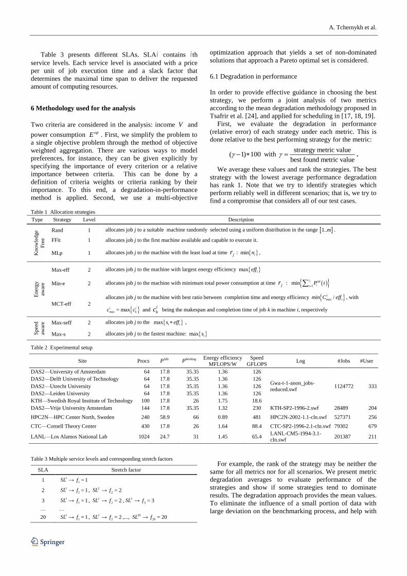
Table 3 presents different SLAs. SLA i contains i th
service levels. Each service level is associated with a price
per unit of job execution time and a slack factor that
determines the maximal time span to deliver the requested
amount of computing resources.
6 Methodology used for the analysis
Two criteria are considered in the analysis: income V and
power consumption opE . First, we simplify the problem to
a single objective problem through the method of objective
weighted aggregation. There are various ways to model
preferences, for instance, they can be given explicitly by
specifying the importance of every criterion or a relative
importance between criteria. This can be done by a
definition of criteria weights or criteria ranking by their
importance. To this end, a degradation-in-performance
method is applied. Second, we use a multi-objective
optimization approach that yields a set of non-dominated
solutions that approach a Pareto optimal set is considered.
6.1 Degradation in performance
In order to provide effective guidance in choosing the best
strategy, we perform a joint analysis of two metrics
according to the mean degradation methodology proposed in
Tsafrir et al. [24], and applied for scheduling in [17, 18, 19].
First, we evaluate the degradation in performance
(relative error) of each strategy under each metric. This is
done relative to the best performing strategy for the metric:
100)1( with strategy metric value
best found metric value .
We average these values and rank the strategies. The best
strategy with the lowest average performance degradation
has rank 1. Note that we try to identify strategies which
perform reliably well in different scenarios; that is, we try to
find a compromise that considers all of our test cases.
Table 1 Allocation strategies
Type Strategy Level Description
Kn
ow
led
ge
Fre
e
Rand 1 allocates job j to a suitable machine randomly selected using a uniform distribution in the range 1..m .
FFit 1 allocates job j to the first machine available and capable to execute it.
MLp 1 allocates job j to the machine with the least load at time jr : min in ,
En
erg
y
awar
e
Max-eff 2 allocates job j to the machine with largest energy efficiency max ieff
Min-e 2 allocates job j to the machine with minimum total power consumption at time jr : 1min
jr op
itP t
MCT-eff 2
allocates job j to the machine with best ratio between completion time and energy efficiency /i
max imin C eff , with
maxi i
max kc = c and i
kc being the makespan and completion time of job k in machine i, respectively
Sp
eed
awar
e Max-seff 2 allocates job j to the max i is eff ,
Max-s 2 allocates job j to the fastest machine: max is
Table 2 Experimental setup
Site Procs Energy efficiency
MFLOPS/W
Speed
GFLOPS Log #Jobs #User
IdleP WorkingP
DAS2—University of Amsterdam 64 17.8 35.35 1.36 126
Gwa-t-1-anon_jobs-
reduced.swf 1124772 333
DAS2—Delft University of Technology 64 17.8 35.35 1.36 126
DAS2—Utrecht University 64 17.8 35.35 1.36 126
DAS2—Leiden University 64 17.8 35.35 1.36 126
KTH—Swedish Royal Institute of Technology 100 17.8 26 1.75 18.6
DAS2—Vrije University Amsterdam 144 17.8 35.35 1.32 230 KTH-SP2-1996-2.swf 28489 204
HPC2N—HPC Center North, Sweden 240 58.9 66 0.89 481 HPC2N-2002-1.1-cln.swf 527371 256
CTC—Cornell Theory Center 430 17.8 26 1.64 88.4 CTC-SP2-1996-2.1-cln.swf 79302 679
LANL—Los Alamos National Lab 1024 24.7 31 1.45 65.4 LANL-CM5-1994-3.1-cln.swf
201387 211
Table 3 Multiple service levels and corresponding stretch factors
SLA Stretch factor
1 1SL →
1 1f =
2 1SL → 1 1f = ,
2SL → 2 2f =
3 1SL → 1 1f = ,
2SL → 2 2f = ,3SL → 3 3f =
… …
20 1SL → 1 1f = ,
2SL → 2 2f = ,..., 20SL → 20 20f =
For example, the rank of the strategy may be neither the
same for all metrics nor for all scenarios. We present metric
degradation averages to evaluate performance of the
strategies and show if some strategies tend to dominate
results. The degradation approach provides the mean values.
To eliminate the influence of a small portion of data with
large deviation on the benchmarking process, and help with

Online Bi-Objective Scheduling for IaaS Clouds with Ensuring Quality of Service
the interpretation of the data, we present performance
profiles of our strategies.
6.2 Performance profile
The performance profile ( ) is a non-decreasing,
piecewise constant function that presents the probability that
a ratio is within a factor of the best ratio [20]. The
function )( is the cumulative distribution function.
Strategies with large probability )( for small will be
preferred.
6.3 Bi-objective analysis
Multi-objective optimization usually finds a set of solution
known as a Pareto optimal set [27]. One solution may
represent a very good solution concerning energy
consumption while another solution may be a very good
solution with respect to the income.
The goal is to choose the most adequate solution and
obtain a set of compromise solutions that represent a good
approximation to the Pareto front. Two important
characteristics of a good multiobjective technique are
convergence to the Pareto front and diversity to sample the
front as fully as possible. A solution is Pareto optimal if no
other solution improves it in terms of all objective functions.
Any solution not belonging to the front can be considered of
inferior quality to those that are included. The selection
between the solutions included in the Pareto front depends
on the system preference. If one objective is considered
more important than the other one then preference is given
to those solutions that are near-optimal in the preferred
objective, even if values of the secondary objective are not
among the best obtained.
Often, results fom multi-objectives problems are
compared via visual observation of the solution space. A
more formal and statistical approach uses a set coverage
metric [20]: given two sets of solutions A and B, the metric
SC(A,B) calculates the proportion of solutions in B, which
are weakly dominated by solutions of A:
{ | : }b B; a A a b
SC A,BB
A metric value SC(A,B) = 1 means that all solutions of B
are dominated by A, whereas SC(A,B) = 0 means that no
member of B is dominated by A. This way, the larger the
value of SC(A,B), the better the Pareto front A with respect to
B. Since the dominance operator is not symmetric, SC(A,B)
is not necessarily equal to 1SC(A,B), and both SC(A,B) and
SC(B,A) have to be computed for understanding how many
solutions of A are covered by B and vice versa.
7 Experimental validation: degradation in performance.
This section reports the experimental analysis of the
proposed schedulers regarding performance degradation.
We study three scenarios: single service level, four service
levels, and the more general multiple service level-multiple
machine, with five different SLAs and up to five service
levels.
7.1 Experimental scenario 1: single service level
Three case-studies are reported: i) in the Case 7.1.1, we use
one SL for all jobs. We vary SL from 1 to 20 to compare our
algorithms with different SLs, and with worst case bound
found on theoretical analysis; ii) in the Case 7.1.2, for a
more detail analysis, we restrict ourself to the SLA 4, where
each job can have one of four SL from the set 1 4SL= SL ,…,SL with slack factors 1 41, 4f = …, f = , and
iii) in the Case 7.1.3, we present a more comprehensive
study varying SLAs from 1 to 5, first considering
degradation of the income and energy consumption, for each
SLA independently, then their means and ranking.
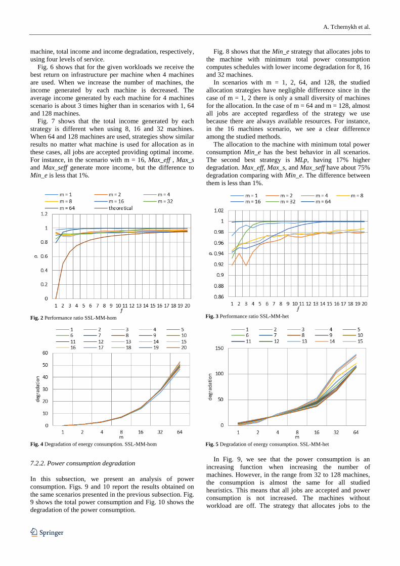
7.1.1 Single service level-multiple machines
Fig. 2 presents the competitive factor in a homogeneous
environment varying stretch factor f. We see that increasing
deadlines for all jobs reduces total income but increases the
flexibility of the scheduler to build schedules closed to the
optimal income. With f = 20 the competitive factors are
close to the optimal. This happens when f becomes large
enough to create a significant difference between job
deadlines and their processing times. For the scenario with
m=64, the competitive factor increases from 8.0ρ with
1f to 1ρ with 5f .
Fig. 3 presents ρ with varying f in a heterogeneous
environment. We see the same tendency of increasing ρ
with increasing f, however, with a higher variation.
Fig. 4 and 5 show the degradation of energy consumption in
homogeneous and heterogeneous environments.
Degradation increases when f grows. We clearly see that
heterogeneity degrades performance slightly more than
twice in energy consumption. In a homogeneous scenario,
the strategies perform almost identically, while the
heterogeneous scenario degrades performance with more
variance.
7.2. Experimental scenario 2: four service levels
All users use a SLA with four service levels with
corresponding slack factors 1 41, 4f = …, f = .
We report four studies: i) in Case 7.2.1 we analyze the
income degradation; ii) in Case 7.2.2 we study the power
consumption degradation; iii) in Case 7.2.3 we study the
mean degradation in performance; and iv) in Case 7.2.4 we
show an analysis of the performance profile.
7.2.1. Income degradation
In this subsection we analyze the income obtained by the
eight allocation strategies studied over the eight considered
infrastructures. Figs. 6 to 8 report the average income per
A. Tchernykh et al.
machine, total income and income degradation, respectively,
using four levels of service.
Fig. 6 shows that for the given workloads we receive the
best return on infrastructure per machine when 4 machines
are used. When we increase the number of machines, the
income generated by each machine is decreased. The
average income generated by each machine for 4 machines
scenario is about 3 times higher than in scenarios with 1, 64
and 128 machines.
Fig. 7 shows that the total income generated by each
strategy is different when using 8, 16 and 32 machines.
When 64 and 128 machines are used, strategies show similar
results no matter what machine is used for allocation as in
these cases, all jobs are accepted providing optimal income.
For instance, in the scenario with m = 16, Max_eff , Max_s
and Max_seff generate more income, but the difference to
Min_e is less that 1%.
Fig. 8 shows that the Min_e strategy that allocates jobs to
the machine with minimum total power consumption
computes schedules with lower income degradation for 8, 16
and 32 machines.
In scenarios with m = 1, 2, 64, and 128, the studied
allocation strategies have negligible difference since in the
case of m = 1, 2 there is only a small diversity of machines
for the allocation. In the case of m = 64 and m = 128, almost
all jobs are accepted regardless of the strategy we use
because there are always available resources. For instance,
in the 16 machines scenario, we see a clear difference
among the studied methods.
The allocation to the machine with minimum total power
consumption Min_e has the best behavior in all scenarios.
The second best strategy is MLp, having 17% higher
degradation. Max_eff, Max_s, and Max_seff have about 75%
degradation comparing with Min_e. The difference between
them is less than 1%.
Fig. 2 Performance ratio SSL-MM-hom
Fig. 3 Performance ratio SSL-MM-het
Fig. 4 Degradation of energy consumption. SSL-MM-hom
Fig. 5 Degradation of energy consumption. SSL-MM-het
7.2.2. Power consumption degradation
In this subsection, we present an analysis of power
consumption. Figs. 9 and 10 report the results obtained on
the same scenarios presented in the previous subsection. Fig.
9 shows the total power consumption and Fig. 10 shows the
degradation of the power consumption.
In Fig. 9, we see that the power consumption is an
increasing function when increasing the number of
machines. However, in the range from 32 to 128 machines,
the consumption is almost the same for all studied
heuristics. This means that all jobs are accepted and power
consumption is not increased. The machines without
workload are off. The strategy that allocates jobs to the

Online Bi-Objective Scheduling for IaaS Clouds with Ensuring Quality of Service
machine with lower total power consumption is about four
times better than the strategy that assigns jobs to the fastest
machine.
From the results, we see that as we increase the number
of service levels in the SLA, the power consumption is
increased slightly and the degradation is a bit higher than in
the scenarios with lower SLAs.
The results on Fig. 10 demonstrate that the degradation in
the scenario with 128 machines is decreased with respect to
64 machines. With more machines, the strategies have more
options for resource allocation, and, in overall, all strategies
take advantage of this diversity. The Min_e strategy has the
best behavior to minimize energy consumption.
7.2.3. Mean degradation in performance analysis.
In the previous subsections, we presented an analysis of the
income and power consumption separately. Now, we are
interested in finding the strategy that generates the best
compromise between income and energy consumption. To
perform this analysis, we use the technique of degradations
and ranking, and performance profile described in Sections
6.1 and 6.2.
Fig. 6 Average income per machine using SLA with 4 service levels.
Fig. 7 Total income using SLA with service levels.
Fig. 8 Income degra dation using SLA with 4 service levels.
Fig. 9 Total power consumption using SLA with 4 SLs
Fig. 10 Degradation of the power consumption using SLA with 4 SLs
Table 4 Degradations and ranking, SLA 4
Str
ateg
y
Inco
me
En
erg
y
Mea
n
Ran
k I
Ran
k E
Ran
k
FFit 0.59 1.52 1.06 5 4 4
Max_s 0.60 2.32 1.46 7 6 6
Max_eff 0.60 1.75 1.18 8 8 8
Max_seff 0.60 2.20 1.40 6 7 7
MCT_eff 0.59 1.61 1.10 3 5 5
Random 0.59 1.30 0.94 4 3 3
Min_e 0.54 0.84 0.69 1 1 1
MLp 0.57 1.24 0.91 2 2 2
A. Tchernykh et al.
Table 4 reports the average degradation for a SLA with
four SL for each set of experiments. The last three columns
of the table contain the ranking of each strategy with respect
to income, power, and their mean. Ranking-P is based on the
income degradation. Ranking-E refers to the position in
relation to the degradation of power consumption. Rank is
the position based on the averaging both degradations.We
see that the best strategy for resource allocation is to assign
jobs to the machine that consumes less energy up to the
moment of allocation (Min_e). This leads to better average
income and lower power consumption. The good performance of this strategy is due to a load
balancing between machines considering total power
consumption. A machine can have lower power
consumption due to various reasons: the machine may
receive fewer loads than other ones; it may have better
energy efficiency, or both. All situations cause load
balancing and generate more income and less power
consumption.
The second best strategy, MLp, assigns jobs to the
machine having less allocated jobs. It also intends to balance
load but this balance is in relation to the assigned work.
The analysis shows that if we have no information about
the speed of the machines or their energy efficiency, it is
better to allocate jobs to the machine that has fewer
assignments. If we have information about speed and energy
efficiency, the best option is assigning a job to the machine
that has consumed less power at the time of the decision.
7.2.4 Performance profile
As mentioned in Section 6.1, conclusions based on the
averages may have some negative aspects. To analyze
effects of allowing a small portion of problem instances with
large deviation to dominate the conclusions that are based
on averages, we present performance profiles of our
strategies.
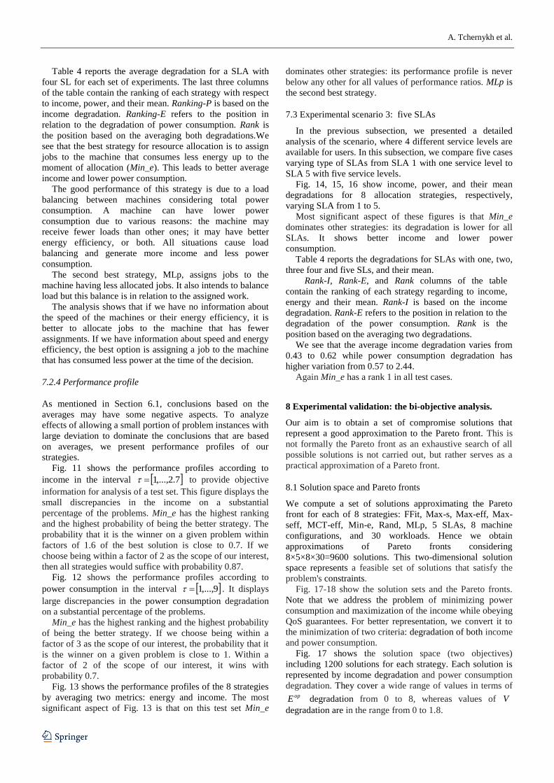
Fig. 11 shows the performance profiles according to
income in the interval 7.2,...,1 to provide objective
information for analysis of a test set. This figure displays the
small discrepancies in the income on a substantial
percentage of the problems. Min_e has the highest ranking
and the highest probability of being the better strategy. The
probability that it is the winner on a given problem within
factors of 1.6 of the best solution is close to 0.7. If we
choose being within a factor of 2 as the scope of our interest,
then all strategies would suffice with probability 0.87.
Fig. 12 shows the performance profiles according to
power consumption in the interval 9,...,1 . It displays
large discrepancies in the power consumption degradation
on a substantial percentage of the problems.
Min_e has the highest ranking and the highest probability
of being the better strategy. If we choose being within a
factor of 3 as the scope of our interest, the probability that it
is the winner on a given problem is close to 1. Within a
factor of 2 of the scope of our interest, it wins with
probability 0.7.
Fig. 13 shows the performance profiles of the 8 strategies
by averaging two metrics: energy and income. The most
significant aspect of Fig. 13 is that on this test set Min_e
dominates other strategies: its performance profile is never
below any other for all values of performance ratios. MLp is
the second best strategy.
7.3 Experimental scenario 3: five SLAs
In the previous subsection, we presented a detailed
analysis of the scenario, where 4 different service levels are
available for users. In this subsection, we compare five cases
varying type of SLAs from SLA 1 with one service level to
SLA 5 with five service levels.
Fig. 14, 15, 16 show income, power, and their mean
degradations for 8 allocation strategies, respectively,
varying SLA from 1 to 5.
Most significant aspect of these figures is that Min_e
dominates other strategies: its degradation is lower for all
SLAs. It shows better income and lower power
consumption.
Table 4 reports the degradations for SLAs with one, two,
three four and five SLs, and their mean.
Rank-I, Rank-E, and Rank columns of the table
contain the ranking of each strategy regarding to income,
energy and their mean. Rank-I is based on the income
degradation. Rank-E refers to the position in relation to the
degradation of the power consumption. Rank is the
position based on the averaging two degradations.
We see that the average income degradation varies from
0.43 to 0.62 while power consumption degradation has
higher variation from 0.57 to 2.44.
Again Min_e has a rank 1 in all test cases.
8 Experimental validation: the bi-objective analysis.
Our aim is to obtain a set of compromise solutions that
represent a good approximation to the Pareto front. This is
not formally the Pareto front as an exhaustive search of all
possible solutions is not carried out, but rather serves as a
practical approximation of a Pareto front.
8.1 Solution space and Pareto fronts
We compute a set of solutions approximating the Pareto
front for each of 8 strategies: FFit, Max-s, Max-eff, Max-
seff, MCT-eff, Min-e, Rand, MLp, 5 SLAs, 8 machine
configurations, and 30 workloads. Hence we obtain
approximations of Pareto fronts considering
8×5×8×30=9600 solutions. This two-dimensional solution
space represents a feasible set of solutions that satisfy the
problem's constraints.
Fig. 17-18 show the solution sets and the Pareto fronts.
Note that we address the problem of minimizing power
consumption and maximization of the income while obeying
QoS guarantees. For better representation, we convert it to
the minimization of two criteria: degradation of both income
and power consumption.
Fig. 17 shows the solution space (two objectives)
including 1200 solutions for each strategy. Each solution is
represented by income degradation and power consumption
degradation. They cover a wide range of values in terms of opE degradation from 0 to 8, whereas values of V
degradation are in the range from 0 to 1.8.
Online Bi-Objective Scheduling for IaaS Clouds with Ensuring Quality of Service
Fig. 18 shows the eight approximations of Pareto fronts
generated by the studied strategies. They cover power
consumption degradations from 0 to 1.8, and income
degradations from 0 to 1.6.
It can be seen that Min-e, MLp and FFit are located in the
lower-left corner, being among the best solutions in terms of
both objectives. They noticeably outperform MCT-eff.
However, we should not consider only Pareto fronts.
When many of the solutions are outside the Pareto front, the
algorithm's performance is variable. This is the case of FFit:
although the Pareto front is of high quality, many of the
generated solutions are quite far from it, and, hence, a single
run of the algorithm may produce significantly worse
results. FFit solutions cover opE degradations from 0 to 6,
whereas Min-e solutions are in the range from 0 to 3.3 of opE degradations.
Fig. 11 Performance profile of the income, 8 strategies
Fig. 12 Performance profile of the energy consumption, 8 strategies
Fig. 13 Performance profile of the power consumption and income average,
8 allocation strategies.
Fig. 14. Average income degradation, varying SLA, 8 allocation strategies
Fig. 15 Average power consumption degradation, varying SLA, 8
allocation strategies
Fig. 16 Mean degradation, varying SLA, 8 allocation strategies
A. Tchernykh et al.
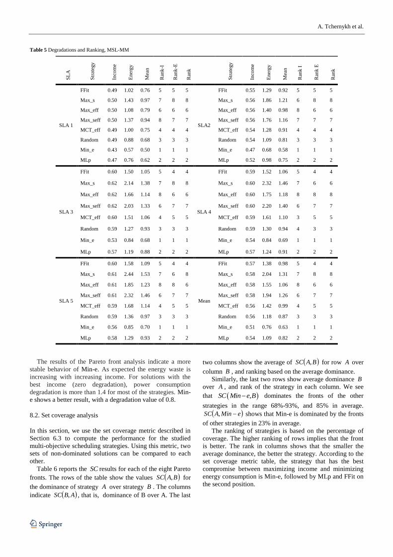
Table 5 Degradations and Ranking, MSL-MM
SL
A
Str
ateg
y
Inco
me
En
erg
y
Mea
n
Ran
k-I
Ran
k-E
Ran
k
Str
ateg
y
Inco
me
En
erg
y
Mea
n
Ran
k I
Ran
k E
Ran
k
SLA 1
FFit 0.49 1.02 0.76 5 5 5
SLA2
FFit 0.55 1.29 0.92 5 5 5
Max_s 0.50 1.43 0.97 7 8 8 Max_s 0.56 1.86 1.21 6 8 8
Max_eff 0.50 1.08 0.79 6 6 6 Max_eff 0.56 1.40 0.98 8 6 6
Max_seff 0.50 1.37 0.94 8 7 7 Max_seff 0.56 1.76 1.16 7 7 7
MCT_eff 0.49 1.00 0.75 4 4 4 MCT_eff 0.54 1.28 0.91 4 4 4
Random 0.49 0.88 0.68 3 3 3 Random 0.54 1.09 0.81 3 3 3
Min_e 0.43 0.57 0.50 1 1 1 Min_e 0.47 0.68 0.58 1 1 1
MLp 0.47 0.76 0.62 2 2 2 MLp 0.52 0.98 0.75 2 2 2
SLA 3
FFit 0.60 1.50 1.05 5 4 4
SLA 4
FFit 0.59 1.52 1.06 5 4 4
Max_s 0.62 2.14 1.38 7 8 8 Max_s 0.60 2.32 1.46 7 6 6
Max_eff 0.62 1.66 1.14 8 6 6 Max_eff 0.60 1.75 1.18 8 8 8
Max_seff 0.62 2.03 1.33 6 7 7 Max_seff 0.60 2.20 1.40 6 7 7
MCT_eff 0.60 1.51 1.06 4 5 5 MCT_eff 0.59 1.61 1.10 3 5 5
Random 0.59 1.27 0.93 3 3 3 Random 0.59 1.30 0.94 4 3 3
Min_e 0.53 0.84 0.68 1 1 1 Min_e 0.54 0.84 0.69 1 1 1
MLp 0.57 1.19 0.88 2 2 2 MLp 0.57 1.24 0.91 2 2 2
SLA 5
FFit 0.60 1.58 1.09 5 4 4
Mean
FFit 0.57 1.38 0.98 5 4 4
Max_s 0.61 2.44 1.53 7 6 8 Max_s 0.58 2.04 1.31 7 8 8
Max_eff 0.61 1.85 1.23 8 8 6 Max_eff 0.58 1.55 1.06 8 6 6
Max_seff 0.61 2.32 1.46 6 7 7 Max_seff 0.58 1.94 1.26 6 7 7
MCT_eff 0.59 1.68 1.14 4 5 5 MCT_eff 0.56 1.42 0.99 4 5 5
Random 0.59 1.36 0.97 3 3 3 Random 0.56 1.18 0.87 3 3 3
Min_e 0.56 0.85 0.70 1 1 1 Min_e 0.51 0.76 0.63 1 1 1
MLp 0.58 1.29 0.93 2 2 2 MLp 0.54 1.09 0.82 2 2 2
The results of the Pareto front analysis indicate a more
stable behavior of Min-e. As expected the energy waste is
increasing with increasing income. For solutions with the
best income (zero degradation), power consumption
degradation is more than 1.4 for most of the strategies. Min-
e shows a better result, with a degradation value of 0.8.
8.2. Set coverage analysis
In this section, we use the set coverage metric described in
Section 6.3 to compute the performance for the studied
multi-objective scheduling strategies. Using this metric, two
sets of non-dominated solutions can be compared to each
other.
Table 6 reports the SC results for each of the eight Pareto
fronts. The rows of the table show the values BA,SC for
the dominance of strategy A over strategy B . The columns
indicate AB,SC , that is, dominance of B over A. The last
two columns show the average of BA,SC for row A over
column B , and ranking based on the average dominance.
Similarly, the last two rows show average dominance B
over A , and rank of the strategy in each column. We see
that SC Min e,B dominates the fronts of the other
strategies in the range 68%-93%, and 85% in average.
eMinASC , shows that Min-e is dominated by the fronts
of other strategies in 23% in average.
The ranking of strategies is based on the percentage of
coverage. The higher ranking of rows implies that the front
is better. The rank in columns shows that the smaller the
average dominance, the better the strategy. According to the
set coverage metric table, the strategy that has the best
compromise between maximizing income and minimizing
energy consumption is Min-e, followed by MLp and FFit on
the second position.

Online Bi-Objective Scheduling for IaaS Clouds with Ensuring Quality of Service
Fig. 17 The solution sets
Fig. 18 The Pareto fronts
Table 6 Set coverage and ranking
B
A
FF
it
Max
-s
Max
-eff
Max
-sef
f
MC
T-e
ff
Min
-e
Ran
do
m
ML
p
Mea
n
Ran
kin
g
FFit 1.00 0.92 0.92 0.92 0.93 0.40 0.39 0.26 0.68 2
seMax-s 0.19 1.00 1.00 1.00 0.20 0.13 0.11 0.16 0.40 4
Max-eff 0.19 1.00 1.00 1.00 0.20 0.13 0.11 0.16 0.40 4
Max-seff 0.19 1.00 1.00 1.00 0.20 0.13 0.11 0.16 0.40 4
MCT-eff 0.11 0.70 0.68 0.71 1.00 0.13 0.07 0.13 0.36 5
Min-e 0.70 0.97 0.95 0.97 0.93 1.00 0.68 0.74 0.85 1
Rand 0.26 0.95 0.92 0.95 0.90 0.33 1.00 0.26 0.65 3
MLp 0.33 0.95 0.89 0.92 0.90 0.33 0.39 1.00 0.67 2
Mean 0.28 0.93 0.91 0.92 0.61 0.23 0.27 0.27
Ranking 3 7 5 6 4 1 2 2
9 Conclusions
In this paper, we analyze a variety of scheduling algorithms
with different cloud configurations and workloads
considering two objectives: provider income and power
consumption.
In our problem model, a user submits jobs to the service
provider, which offers several levels of service. For a given
service level the user is charged a cost per unit of execution
time. In return, the user receives guarantees regarding the
provided resources: lower service level – higher cost. The
maximum response time (deadline) used as QoS constraints.
Our experimental analysis on several cases of study
results in several contributions:
(a) We identify the problem of the resource allocation
with several service levels and quality of service to make
scheduling decisions with respect to job acceptance and two
criteria optimization;
(b) We analyze scenarios with homogeneous and
heterogeneous machines of different configurations and
workloads;
(c) We provide a comprehensive experimental study of
greedy acceptance algorithms with known worst case
performance bound and 8 allocation strategies that take into
account heterogeneity of the environment: knowledge free,
energy-aware, and speed-aware;
(e) To provide effective guidance in choosing a good
strategy, we perform a joint analysis of two conflicting goals
first based on the degradation in performance of each
strategy under each metric; then based on the Pareto front
and set coverage metric.
(f) Simulation results presented in the paper reveal that in
terms of minimizing power consumption and maximization
of the provider income Min_e allocation strategy
outperforms other algorithms. It dominates in almost all test
cases. We conclude that the strategy is stable even under
significantly different conditions. It provides minor
performance degradation and copes with different demands.
Min_e provides major dominance with a set coverage
metric. We find that the information about the speed of
machines does not help to improve significantly the
allocation strategies.
A. Tchernykh et al.
(i) The final result suggests a simple allocation strategy,
which requires minimal information and little computational
complexity; nevertheless, it achieves good improvements in
our objectives and provides quality of service guarantees.
However, further study for multiple service classes is
required to assess its actual efficiency and effectiveness.
This will be subject of future work for better understanding
of service levels, QoS and multi-objective optimization in
IaaS clouds.
Acknowledgment. This work is partially supported by CONACYT
(Consejo Nacional de Ciencia y Tecnología, México), grant no. 178415.
The work of S. Nesmachnow is partly funded by ANII and PEDECIBA, Uruguay. The work of P. Bouvry and J. Pecero is partly funded by
INTER/CNRS/11/03 Green@Cloud. Drozdov is supported by the Ministry
of Education and Science of Russian Federation under contract No02.G25.31.0061 12/02/2013 (Government Regulation No 218 from
09/04/2010).
References
1. Ahmad, I., Ranka, S.: Handbook of Energy-Aware and Green
Computing, Chapman & Hall/CRC (2012) 2. Zomaya, Y., Lee, Y.: Energy Efficient Distributed Computing
Systems, Wiley-IEEE Computer Society Press (2012)
3. Lezama, A., Tchernykh, A., Yahyapour, R.: Performance Evaluation of Infrastructure as a Service Clouds with SLA Constraints.
Computación y Sistemas 17(3): 401–411 (2013)
4. Schwiegelshohn, U., Tchernykh, A.: Online Scheduling for Cloud Computing and Different Service Levels, 26th Int. Parallel and
Distributed Processing Symposium Los Alamitos, CA, pp. 1067–1074
(2012) 5. Tchernykh, A., Pecero, J., Barrondo, A., Schaeffer, E.: Adaptive
Energy Efficient Scheduling in Peer-to-Peer Desktop Grids, Future
Generation Computer Systems, 36:209–220 (2014). 6. Raycroft, P., Jansen, R., Jarus, M., Brenner, P.: Performance bounded
energy efficient virtual machine allocation in the global cloud,
Sustainable Computing: Informatics and Systems 4(1):1–9 (2014) 7. Khan, S., Ahmad, I.: A cooperative game theoretical technique for
joint optimization of power consumption and response time in computational grids. Transactions on Parallel and Distributed
Systems 20(3):346–360 (2009)
8. Lee, Y., Zomaya, A.: Energy conscious scheduling for distributed computing systems under different operating conditions, IEEE
Transactions on Parallel and Distributed Systems 22(8):1374–1381
(2011) 9. Mezmaz, M., Melab, N., Kessaci, Y., Lee, Y., Talbi, E., Zomaya, A.,
Tuyttens, D.: A parallel bi-objective hybrid metaheuristic for energy-
aware scheduling for cloud computing systems. Journal of Parallel and Distributed Computing 71(11):1497–1508 (2011)
10. Pecero, J., Bouvry, P., Fraire, H., Khan, S.: A multi-objective GRASP
algorithm for joint optimization of power consumption and schedule length of precedence-constrained applications”. International
Conference on Cloud and Green Computing, pp. 1–8 (2011)
11. Lindberg, P., Leingang, J., Lysaker, D., Khan, S., Li, J.: Comparison and analysis of eight scheduling heuristics for the optimization of
power consumption and makespan in large-scale distributed systems.
Journal of Supercomputing 59(1):323–360 (2012). 12. Nesmachnow, S., Dorronsoro, B., Pecero, J., Bouvry, P.: Energy-
Aware Scheduling on Multicore Heterogeneous Grid Computing
Systems. Journal of Grid Computing 11(4):653–680 (2013) 13. Iturriaga, S., Nesmachnow, S., Dorronsoro, B., Bouvry, P.: Energy
efficient scheduling in heterogeneous systems with a parallel
multiobjective local search. Computing and Informatics 32(2):273–294 (2013)
14. DasGupta, B., Palis, M.: Online Real-time Preemptive Scheduling of
Jobs with Deadlines on Multiple Machines, Scheduling 4(6), 297-312 (2001)
15. Parallel Workload Archive [Online, November 2014]. Available at
http://www.cs.huji.ac.il/labs/parallel/workload
16. Grid Workloads Archive [Online, November 2014]. Available at
http://gwa.ewi.tudelft.nl 17. Ramírez, J.M., Tchernykh, A., Yahyapour, R., Schwiegelshohn, U.,
Quezada, A., González, J., Hirales, A.: Job Allocation Strategies with
User Run Time Estimates for Online Scheduling in Hierarchical Grids. Journal of Grid Computing 9:95–116 (2011)
18. Quezada, A., Tchernykh, A., González, J., Hirales, A., Ramírez, J.-
M., Schwiegelshohn, U., Yahyapour, R., Miranda, V.: Adaptive parallel job scheduling with resource admissible allocation on two-
level hierarchical grids. Future Generation Computer Systems 28(7):
965–976 (2012) 19. Tchernykh, A., Lozano, L., Schwiegelshohn, U., Bouvry, P., Pecero,
J. E., Nesmachnow, S.: Energy-Aware Online Scheduling: Ensuring
Quality of Service for IaaS Clouds. International Conference on High Performance Computing & Simulation (HPCS 2014), pp 911–918,
Bologna, Italy (2014)
20. Zitzler, E.: Evolutionary algorithms for multiobjective optimization: Methods and applications, PhD thesis, Swiss Federal Institute of
Technology. Zurich (1999)
21. Tchernykh, A., Lozano, L., Schwiegelshohn, U., Bouvry, P., Pecero, J. E., Nesmachnow, S.: Bi-Objective Online Scheduling with Quality
of Service for IaaS Clouds. In 3rd IEEE International Conference on
Cloud Networking, Luxembourg (2014) 22. Tchernykh, A., Schwiegelsohn, U., Yahyapour, R., Kuzjurin, N.:
Online Hierarchical Job Scheduling on Grids with Admissible
Allocation, Journal of Scheduling 13(5):545–552 (2010) 23. Tchernykh, A., Ramírez, J., Avetisyan, A., Kuzjurin, N., Grushin, D.,.
Zhuk, S.: Two Level Job-Scheduling Strategies for a Computational Grid. In R. Wyrzykowski et al. (eds.) Parallel Processing and
Applied Mathematics, 6th International Conference on Parallel
Processing and Applied Mathematics. Poznan, Poland, 2005, LNCS 3911, pp. 774–781, Springer-Verlag (2006)
24. Tsafrir, D., Etsion, Y., Feitelson, D.: Backfilling Using System-
Generated Predictions Rather than User Runtime Estimates. IEEE Transactions on Parallel and Distributed Systems 18 (6), pp.789–803
(2007)
25. Nesmachnow, S., Perfumo, C., Goiri, I.: Controlling datacenter power consumption while maintaining temperature and QoS levels. In: 3rd
IEEE International Conference on Cloud Networking, Luxembourg
(2014) 26. Dorronsoro, B., Nesmachnow, S., Taheri, J., Zomaya, A., Talbi, E-G.,
Bouvry, P.: A hierarchical approach for energy-efficient scheduling of
large workloads in multicore distributed systems. Sustainable Computing: Informatics and Systems 4:252–261 (2014)
27. Deb, K.: Multi-Objective Optimization Using Evolutionary
Algorithms. John Wiley & Sons, Inc., New York, NY, USA (2001) 28. Hirales, A., Tchernykh, A., Roblitz, T., Yahyapour, R.: A Grid
simulation framework to study advance scheduling strategies for
complex workflow applications. Parallel Distributed Processing, Workshops and Phd Forum (IPDPSW), 2010 IEEE International
Symposium on. pp. 1–8 (2010).