LUND UNIVERSITY

PO Box 117221 00 Lund+46 46-222 00 00

Online Minimum-Jerk Trajectory Generation

Ghazaei, Mahdi; Robertsson, Anders; Johansson, Rolf

Published: 2015-01-01

Link to publication

Citation for published version (APA):Ghazaei, M., Robertsson, A., & Johansson, R. (2015). Online Minimum-Jerk Trajectory Generation. Paperpresented at 2015 IMA Conference on Mathematics of Robotics, Oxford, United Kingdom.

General rightsCopyright and moral rights for the publications made accessible in the public portal are retained by the authorsand/or other copyright owners and it is a condition of accessing publications that users recognise and abide by thelegal requirements associated with these rights.

• Users may download and print one copy of any publication from the public portal for the purpose of privatestudy or research. • You may not further distribute the material or use it for any profit-making activity or commercial gain • You may freely distribute the URL identifying the publication in the public portalTake down policyIf you believe that this document breaches copyright please contact us providing details, and we will removeaccess to the work immediately and investigate your claim.

Download date: 14. Sep. 2018

1

Online Minimum-Jerk Trajectory Generation

By M. M. Ghazaei Ardakani, A. Robertsson, R. Johansson†The Department of Automatic Control, LTH, Lund University, SE–221 00 Lund, Sweden

{mahdi.ghazaei, anders.robertsson, rolf.johansson}@control.lth.se

Abstract

Robotic trajectory generation is reformulated as a controller design problem. Forminimum-jerk trajectories, an optimal controller using the Hamilton-Jacobi-Bellmanequation is derived. The controller instantaneously updates the trajectory in a closed-loop system as a result of the changes in the reference signal. The resulting trajectoriescoincide with piece-wise fifth-order polynomial trajectories for piece-wise constant targetstates. Since having hard constraints on the final time poses certain robustness issues,a smooth transition between the finite-horizon and an infinite-horizon problem is devel-oped. This enables to switch softly to a tracking mode when a moving target is reached.

1. Introduction

A fundamental problem in robotics is planning the motion for a task. At the lowest level,a movement is described by a trajectory, i.e., a mapping from the time to the position. Animportant class of motion planning problems is concerned with point-to-point trajectorygeneration. In this case, the objective can for instance be to reach a final state in theminimum time given certain constraints (Macfarlane & Croft 2003; Haschke et al. 2008)or in a fixed time. The fixed-time problems are of importance when a less aggressivestrategy than a minimum-time solution is sufficient. Moreover, fixed-time motions lendthemselves to the coordination between several degrees of freedom or entities.

Several approaches to dealing with fixed-time problems have been suggested. A com-mon approach is fitting a piece-wise polynomial between the starting point and a finalpoint (Taylor 1979; Lin et al. 1983). von Stryk and Schlemmer (1994) suggested the opti-mization of the energy or the power consumption and minimizing the effort was proposedby Martin and Bobrow (1997). The solutions were obtained by numerical methods eitherby discretization or parameter optimization over a set of basis functions. A sub-optimalsolution to the fixed-time trajectory planning considering a more generic cost functionwas derived by Dulcba (1997).

For trajectory generation, polynomials play an important role. They show up for ex-ample as partial solutions to the minimum-time problems or they are used as the basisfunctions. Specially, fifth-order polynomials are solutions to a minimum-jerk model sug-gested by Flash and Hogan (1985). An important feature of this model is that it providesa kinematic description of the motion of the human hand in planar scenarios. The modelis able to predict the bell-shaped velocity profiles in point-to-point movements as wellas the qualitative features of the curvature in via-point movements. According to this

† The authors are members of the LCCC Linnaeus Center and the ELLIIT Excellence Centerat Lund University.

Online Minimum-Jerk Trajectory Generation 2

model, the cost functional to be minimized is:

C =1

2

d0∫0

(...X

2+

...Y

2)dt,

...X :=

d3X

dt3,

...Y :=

d3Y

dt3(1.1)

where X and Y represent the coordinates and d0 the duration of the movement. Assumingthat the X and the Y coordinates are decoupled, it is possible to break (1.1) into twoone-dimensional optimization problems. Using the variational principle, the solution isshown to be a fifth-order polynomial (Shadmehr 2005).

As a motivating example for this article, consider a quadcopter task to follow/catchflying objects as soon as they cross a border. A camera system detects the objects andestimates of the current position, velocity, and acceleration as well as an estimate ofthe arrival of the objects are provided. We choose a minimum-jerk trajectory profile togenerate smooth motion. This application falls under the fixed-time trajectory planning.Moreover, it requires to replan the trajectory online, i.e., as soon as new estimates areobtained.

Earlier works have focused on computationally efficient solutions to time-optimal prob-lems for online trajectory generation (Kroger and Wahl 2010; Hehn and D’Andrea 2011).A generic way to deal with the online trajectory generation is to buffer each segment ofthe trajectory (or its parameters) and implement switching between the pieces. However,this approach becomes inefficient if the update rate of the trajectory is high. Thus, ratherthan considering trajectories as solely a function of time, we propose an alternative viewbased on dynamical systems. This allows for a fully reactive trajectory generation methodwith continuous reactions to the changes in the target.

2. Problem formulation

This article concerns the one-dimensional minimum-jerk trajectory-generation problemgiven a fixed time. The main motivation is to update trajectories immediately as aresult of changes in the (moving) target while ensuring the continuity of the position,velocity and acceleration of the trajectory. Moreover, we require a smooth transitionbetween trajectory planning and tracking modes. In contrast to mathematically designedor optimal trajectories purely as a function of time, we regard a trajectory as an outputof a dynamical system. The exogenous input signal defines the set-point for the trajectorygenerator.

For minimizing the jerk, each decoupled degree of freedom can be represented by atriple integrator. Let u denote the jerk and y(t) the trajectory, thenx1x2

x3

=

0 1 00 0 10 0 0

x1x2x3

+

001

u (2.1)

y = x1. (2.2)

We define the reference signal r(t) ∈ R3 such that r1(t), r2(t), r3(t) denote the currentposition, velocity and acceleration of the target, respectively. Given the reference signalr(t) and the desired time tf , we wish to design u(x, r, t) that produces the solution to

minimizeu

∫ tf

t0

u2 dt (2.3)

subject to (2.1), x(t0) = x0, and x(t) = r(t), for t ≥ tf .

OPTIMAL CONTROLLER 3

3. Optimal Controller

Starting from model (2.1), we have

x =(x2 x3 u

)T:= f(t, x, u). (3.1)

According to the Pontryagin maximum principle (Pontryagin et al. 1962; Liberzon 2011),

x∗ = Hp(x∗, u∗, p, p0) (3.2)

p = −Hx(x∗, u∗, p, p0) (3.3)

x∗(t0) = x0, x∗(tf ) = r(tf ) (3.4)

Here, H denotes the Hamiltonian, the subscripts denote partial derivatives with respectto the given variable, x and p are the states and the costates, respectively, t0 and tfdenote the initial and final time, respectively, and variables with star correspond to theoptimal solution. The optimal control maximizes the Hamiltonian, that is

H(x∗(t), u∗(t), p(t), p0) ≤ H(x∗(t), u, p(t), p0) (3.5)

Denoting the running cost by L(x, u), for problem (2.3), the Hamiltonian is

H(x, u, p, p0) = 〈p, f(x, u)〉+ p0L(x, u) (3.6)

=(p1 p2 p3

)x2x3u

+ p0u2. (3.7)

By the partial differentiation of H with respect to u, we find the extremum to be

∂H

∂u= 2p0u+ p3 = 0⇒ u∗ = − p3

2p0. (3.8)

Consequently, the Hamiltonian along the optimal trajectory is

H(x∗, u∗, p, p0) = p1x∗2 + p2x

∗3 −

p234p0

, (3.9)

where

p1 = −Hx1 = 0 (3.10)

p2 = −Hx2 = −p1 (3.11)

p3 = −Hx3 = −p2. (3.12)

These equations combined with (3.8) give us

u∗ = k1t2 + k2t+ k3, (3.13)

with coefficients k1, k2, and k3 to be determined. Integrating the control signal three timesresults in x1, which is apparently a fifth-order polynomial. For the sake of simplicity, we

Online Minimum-Jerk Trajectory Generation 4

assume t0 = 0 and x(tf ) = 0. By matching the initial and final conditions, we obtain

y = x∗1 = y0(1− 10t3n + 15t4n − 6t5n) + v0d0tn(1− 6t2n + 8t3n − 3t4n) (3.14)

+a02d20t

2n(1− 3tn + 3t2n − t3n)

y = x∗2 =y0d0

(−30t2n + 60t3n − 30t4n) + v0(1− 18t2n + 32t3n − 15t4n) (3.15)

+ a0d0tn(1− 9

2tn + 6t2n −

5

2t3n)

y = x∗3 =y0d20

(−60tn + 180t2n − 120t3n) +v0d0

(−36tn + 96t2n − 60t3n) (3.16)

+ a0(1− 9tn + 18t2n − 10t3n),

and the optimal control signal is

...y = u∗ =

y0d30

(−60 + 360tn − 360t2n) +v0d20

(−36 + 192tn − 180t2n)

+a0d0

(−9 + 36tn − 30t2n) (3.17)

where tn := (t − t0)/d0 is the normalized elapsed time with respect to the durationd0 = tf−t0 and y0, v0, and a0 are initial position, velocity, and acceleration, respectively.

Let us now consider the Hamilton-Jacobi-Bellman (HJB) equation (Bellman & Kalaba1965; Liberzon 2011)

−Vt(t, x) = infu∈U{L(t, x, u) + 〈Vx(t, x), f(t, x, u)〉}, (3.18)

with the cost function J and the value function V defined as

J(t, x, u) :=

∫ tf

t

L(s, x(s), u(s)) ds+K(x(tf )) (3.19)

V (t, x) := infu[t,tf ]

J(t, x, u). (3.20)

Here, U ⊆ R defines the control set, L(·) and K(·) denote the running cost and theterminal cost, respectively. For the minimum-jerk problem, we have

L(t, x, u) = u2, K(x(tf )) = 0 (3.21)

−Vt(t, x) = infu∈U{u2 + 〈Vx(t, x), f(t, x, u)〉} (3.22)

= minu∈R{u2 + Vx1

x2 + Vx2x3 + Vx3

u}. (3.23)

The optimum is achieved for

∂(u2 + Vx1x2 + Vx2

x3 + Vx3u)

∂u= 0⇒ u∗ = −Vx3

2. (3.24)

Therefore,

−Vt(t, x) = −V2x3

4+ Vx1

x2 + Vx2x3. (3.25)

As a result of the application of the maximum principle, (3.17) gives us an expressionfor

...y along the optimal path. Now, considering the value function in (3.20), i.e., the cost

to go, and using the definition of the cost function in (3.19), we conclude

V (t, x) =

∫ tf

t

...y 2(s) ds. (3.26)

SERVO PROBLEM 5

Traj. GeneratorController

Robot+

Modelx

r e u y

−

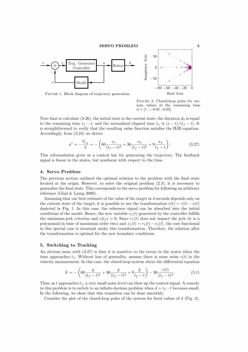
Figure 1. Block diagram of trajectory generation.

−80 −60 −40 −20 0

−50

0

50

Real Axis

Imaginary

Axis

Figure 2. Closed-loop poles for var-ious values of the remaining timed = [1 : −0.05 : 0.05].

Note that to calculate (3.26), the initial state is the current state, the duration d0 is equalto the remaining time tf − t, and the normalized elapsed time tn is (s − t)/(tf − t). Itis straightforward to verify that the resulting value function satisfies the HJB equation.Accordingly, from (3.24) we derive

u∗ = −Vx3

2= −

(60

x1(tf − t)3

+ 36x2

(tf − t)2+ 9

x3tf − t

). (3.27)

This reformulation gives us a control law for generating the trajectory. The feedbacksignal is linear in the states, but nonlinear with respect to the time.

4. Servo Problem

The previous section outlined the optimal solution to the problem with the final statelocated at the origin. However, to solve the original problem (2.3), it is necessary togeneralize the final state. This corresponds to the servo problem for following an arbitraryreference (Glad & Ljung 2000).

Assuming that our best estimate of the value of the target in d seconds depends only onthe current state of the target, it is possible to use the transformation e(t) = r(t)− x(t)depicted in Fig. 1. In this case, the reference signal can be absorbed into the initialconditions of the model. Hence, the new variable e1(t) generated by the controller fulfillsthe minimum-jerk criterion and e(tf ) = 0. Since r1(t) does not impact the jerk (it is apolynomial in time of maximum order two) and x1(t) = r1(t)− e1(t), the cost functionalin this special case is invariant under this transformation. Therefore, the solution afterthe transformation is optimal for the new boundary conditions.

5. Switching to Tracking

An obvious issue with (3.27) is that it is sensitive to the errors in the states when thetime approaches tf . Without loss of generality, assume there is some noise ε(t) in thevelocity measurement. In this case, the closed-loop system obeys the differential equation

...y = −

(60

y

(tf − t)3+ 36

y

(tf − t)2+ 9

y

tf − t

)− 36

ε(t)

(tf − t)2. (5.1)

Thus, as t approaches tf , a very small noise level can blow up the control signal. A remedyto this problem is to switch to an infinite-horizon problem when d = tf−t becomes small.In the following, we show that this transition can be done smoothly.

Consider the plot of the closed-loop poles of the system for fixed values of d (Fig. 2).

Online Minimum-Jerk Trajectory Generation 6

0 0.2 0.4 0.6 0.8 1 1.2

−1

−0.5

0

x(m

)

0 0.2 0.4 0.6 0.8 1 1.2−2

0

2

Time (s)

v(m

/s)

v0 :

−5 0 5a0 :

−2 0 2

−1 −0.5 0

−2

0

2

x (m)

v(m

/s)

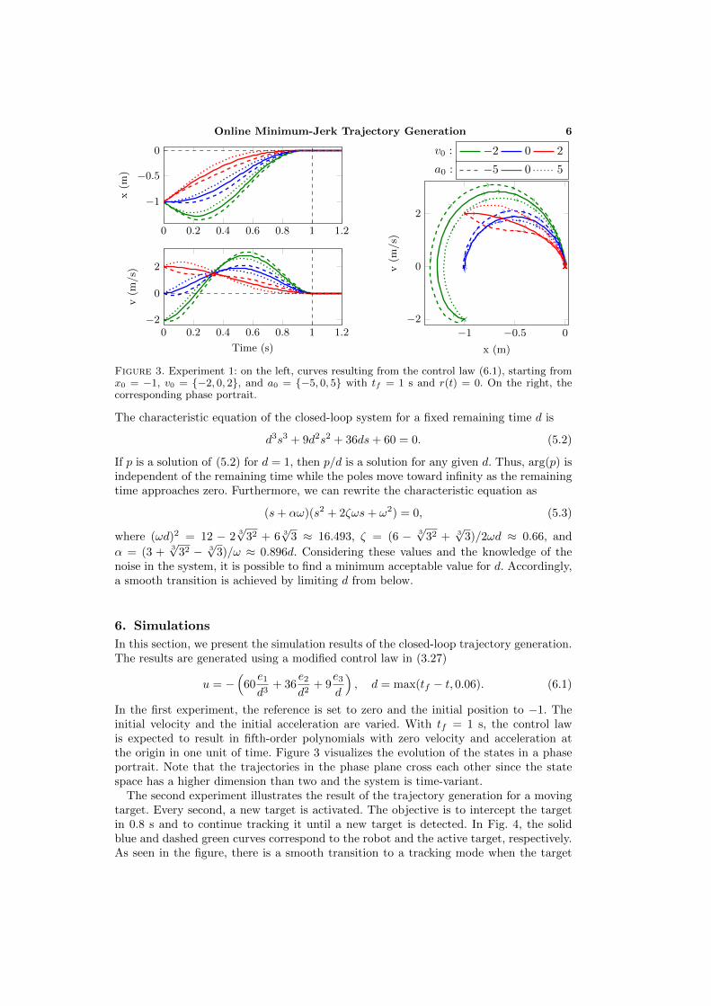
Figure 3. Experiment 1: on the left, curves resulting from the control law (6.1), starting fromx0 = −1, v0 = {−2, 0, 2}, and a0 = {−5, 0, 5} with tf = 1 s and r(t) = 0. On the right, thecorresponding phase portrait.

The characteristic equation of the closed-loop system for a fixed remaining time d is

d3s3 + 9d2s2 + 36ds+ 60 = 0. (5.2)

If p is a solution of (5.2) for d = 1, then p/d is a solution for any given d. Thus, arg(p) isindependent of the remaining time while the poles move toward infinity as the remainingtime approaches zero. Furthermore, we can rewrite the characteristic equation as

(s+ αω)(s2 + 2ζωs+ ω2) = 0, (5.3)

where (ωd)2 = 12 − 23√

32 + 6 3√

3 ≈ 16.493, ζ = (6 − 3√

32 + 3√

3)/2ωd ≈ 0.66, and

α = (3 +3√

32 − 3√

3)/ω ≈ 0.896d. Considering these values and the knowledge of thenoise in the system, it is possible to find a minimum acceptable value for d. Accordingly,a smooth transition is achieved by limiting d from below.

6. Simulations

In this section, we present the simulation results of the closed-loop trajectory generation.The results are generated using a modified control law in (3.27)

u = −(

60e1d3

+ 36e2d2

+ 9e3d

), d = max(tf − t, 0.06). (6.1)

In the first experiment, the reference is set to zero and the initial position to −1. Theinitial velocity and the initial acceleration are varied. With tf = 1 s, the control lawis expected to result in fifth-order polynomials with zero velocity and acceleration atthe origin in one unit of time. Figure 3 visualizes the evolution of the states in a phaseportrait. Note that the trajectories in the phase plane cross each other since the statespace has a higher dimension than two and the system is time-variant.

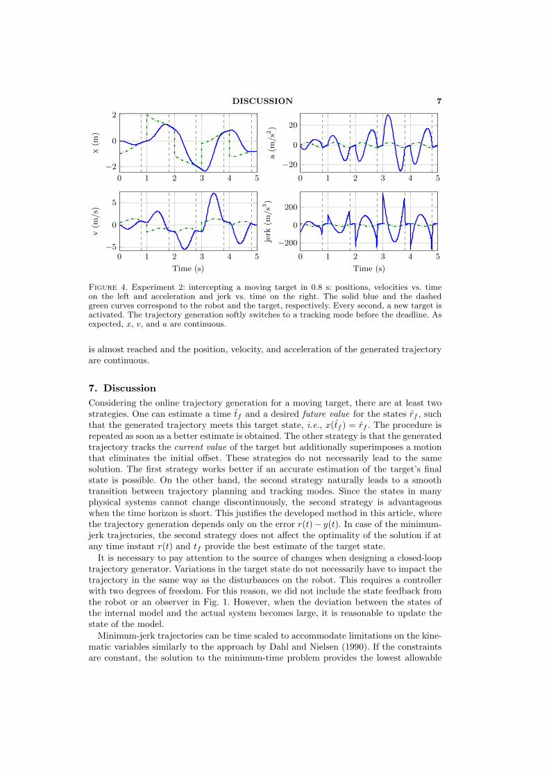
The second experiment illustrates the result of the trajectory generation for a movingtarget. Every second, a new target is activated. The objective is to intercept the targetin 0.8 s and to continue tracking it until a new target is detected. In Fig. 4, the solidblue and dashed green curves correspond to the robot and the active target, respectively.As seen in the figure, there is a smooth transition to a tracking mode when the target

DISCUSSION 7

0 1 2 3 4 5

−2

0

2

x(m

)

0 1 2 3 4 5−5

0

5

Time (s)

v(m

/s)

0 1 2 3 4 5

−20

0

20

a(m

/s2)

0 1 2 3 4 5

−200

0

200

Time (s)jerk

(m/s3)

Figure 4. Experiment 2: intercepting a moving target in 0.8 s: positions, velocities vs. timeon the left and acceleration and jerk vs. time on the right. The solid blue and the dashedgreen curves correspond to the robot and the target, respectively. Every second, a new target isactivated. The trajectory generation softly switches to a tracking mode before the deadline. Asexpected, x, v, and a are continuous.

is almost reached and the position, velocity, and acceleration of the generated trajectoryare continuous.

7. Discussion

Considering the online trajectory generation for a moving target, there are at least twostrategies. One can estimate a time tf and a desired future value for the states rf , suchthat the generated trajectory meets this target state, i.e., x(tf ) = rf . The procedure isrepeated as soon as a better estimate is obtained. The other strategy is that the generatedtrajectory tracks the current value of the target but additionally superimposes a motionthat eliminates the initial offset. These strategies do not necessarily lead to the samesolution. The first strategy works better if an accurate estimation of the target’s finalstate is possible. On the other hand, the second strategy naturally leads to a smoothtransition between trajectory planning and tracking modes. Since the states in manyphysical systems cannot change discontinuously, the second strategy is advantageouswhen the time horizon is short. This justifies the developed method in this article, wherethe trajectory generation depends only on the error r(t)− y(t). In case of the minimum-jerk trajectories, the second strategy does not affect the optimality of the solution if atany time instant r(t) and tf provide the best estimate of the target state.

It is necessary to pay attention to the source of changes when designing a closed-looptrajectory generator. Variations in the target state do not necessarily have to impact thetrajectory in the same way as the disturbances on the robot. This requires a controllerwith two degrees of freedom. For this reason, we did not include the state feedback fromthe robot or an observer in Fig. 1. However, when the deviation between the states ofthe internal model and the actual system becomes large, it is reasonable to update thestate of the model.

Minimum-jerk trajectories can be time scaled to accommodate limitations on the kine-matic variables similarly to the approach by Dahl and Nielsen (1990). If the constraintsare constant, the solution to the minimum-time problem provides the lowest allowable

Online Minimum-Jerk Trajectory Generation 8

tf (Hehn and D’Andrea 2011), i.e., any trajectory generated with a larger time intervalthan the minimum time satisfies the constraints. For more discussion about handlingstate constraints by adjusting the time, see (Ghazaei A. 2015).

8. Conclusions

A controller model for trajectory generation with continuous reactions to the changesin the target is proposed. We solve the Hamilton-Jacobi-Bellman equation in order tofind the optimal minimum-jerk controller. The result is a time-varying linear feedbacklaw, which produces fifth-order polynomials for piece-wise constant target states. Forthis controller, we show that limiting the remaining time from below naturally leads toa smooth transition between trajectory planning and tracking modes. Thus, we haveobtained a fully reactive trajectory generation method for possibly moving targets withthe desirable properties of minimum-jerk trajectories.

REFERENCES

Bellman, R. and Kalaba, R. E. (1965). Dynamic programming and modern control theory.Academic Press, New York.

Dahl, O. and Nielsen, L. (1990). Torque limited path following by on-line trajectory time scaling.IEEE Trans. Rob. and Autom., 6:554–561.

Dulcba, I. (1997). Minimum cost, fixed time trajectory planning in robot manipulators. Asuboptimal solution. Robotica, 15(5):555–562.

Flash, T. and Hogan, N. (1985). The coordination of arm movements: an experimentally con-firmed mathematical model. J. Neuroscience, 5(7):1688–1703.

Ghazaei Ardakani, M. M. (2015). Topics in trajectory generation for robots. Licentiate ThesisTFRT--3265--SE, Dept. Automatic Control, Lund University, Sweden.

Glad, T. and Ljung, L. (2000). Control Theory: Multivariable and Nonlinear Methods. Taylor& Francis, London.

Haschke, R., Weitnauer, E., and Ritter, H. (2008). On-line planning of time-optimal, jerk-limitedtrajectories. In Proc. IEEE/RSJ Int. Conf. Intelligent Robots and Systems (IROS), Sep.22-26, 2008, pages 3248–3253, Nice, France.

Hehn, M. and D’Andrea, R. (2011). Quadrocopter trajectory generation and control. In Proc.18th IFAC World Cong., Aug. 28–Sep. 2, 2011, volume 18, pages 1485–1491, Milano, Italy.

Kroger, T. and Wahl, F. M. (2010). On-line trajectory generation: Basic concepts for instanta-neous reactions to unforeseen events. IEEE Trans. Robot., 26(1):94–111.

Liberzon, D. (2011). Calculus of Variations and Optimal Control Theory: A Concise Introduc-tion. Princeton University Press, Princeton, New Jersey.

Lin, C.-S., Chang, P.-R., and Luh, J. (1983). Formulation and optimization of cubic polynomialjoint trajectories for industrial robots. IEEE Trans. Automatic Control, 28(12):1066–1074.

Macfarlane, S. and Croft, E. A. (2003). Jerk-bounded manipulator trajectory planning: designfor real-time applications. IEEE Trans. Rob. Autom., 19(1):42–52.

Martin, B. J. and Bobrow, J. E. (1997). Minimum effort motions for open chain manipulatorswith task-dependent end-effector constraints. In Proc. IEEE Int. Conf. Rob. and Autom.,Apr. 20–25, 1997, volume 3, pages 2044–2049, Albuquerque, NM.

Pontryagin, L. S., Boltyanskii, V., Gamkrelidze, R., and Mishchenko, E. (1962). The Mathe-matical Theory of Optimal Processes. Interscience, New York.

Shadmehr, R. (2005). The computational neurobiology of reaching and pointing: a foundationfor motor learning. MIT press, Cambridge, MA.

Taylor, R. H. (1979). Planning and execution of straight line manipulator trajectories. IBM J.Research and Development, 23(4):424–436.

von Stryk, O. and Schlemmer, M. (1994). In Bulirsch, R. and Kraft, D., editors, ComputationalOptimal Control, chapter Optimal Control of the Industrial Robot Manutec R3, pages367–382. Birkhauser Verlag, Basel, Switzerland.