Embed Size (px)
Citation preview

Online Path Planning for AUV Rendezvous in Dynamic Cluttered Undersea
Environment Using Evolutionary Algorithms
S.M. Zadeh· A.M. Yazdani· K. Sammut· D.M.W Powers
Centre for Maritime Engineering, Control and Imaging,
School of Computer Science, Engineering and Mathematics, Flinders University, Adelaide, SA 5042, Australia
[email protected] [email protected]
Abstract- In this study, a single autonomous underwater vehicle (AUV) aims to rendezvous with a submerged leader
recovery vehicle through a cluttered and variable operating field. The rendezvous problem is transformed into a Nonlinear
Optimal Control Problem (NOCP) and then numerical solutions are provided. A penalty function method is utilized to
combine the boundary conditions, vehicular and environmental constraints with the performance index that is final
rendezvous time. Four evolutionary based path planning methods namely Particle Swarm Optimization (PSO),
Biogeography-Based Optimization (BBO), Differential Evolution (DE), and Firefly Algorithm (FA) are employed to
establish a reactive planner module and provide a numerical solution for the proposed NOCP. The objective is to synthesize
and analyze the performance and capability of the mentioned methods for guiding an AUV from an initial loitering point
toward the rendezvous through a comprehensive simulation study. The proposed planner module entails a heuristic for
refining the path considering situational awareness of environment, encompassing static and dynamic obstacles within a
spatiotemporal current fields. The planner thus needs to accommodate the unforeseen changes in the operating field such as
emergence of unpredicted obstacles or variability of current field and turbulent regions. The simulation results demonstrate
the inherent robustness and efficiency of the proposed planner for enhancing a vehicle’s autonomy so as to enable it to
reach the desired rendezvous. The advantages and shortcoming of all utilized methods are also presented based on the
obtained results.
Keywords- Rendezvous, nonlinear optimal control problem, reactive path planning, autonomous underwater vehicles,
evolutionary algorithms
1 Introduction
AUV rendezvous with a mother ship, mobile recovery station or submerged vehicle has been an area of interest in recent
underwater surveys and oceanic exploration [1-3]. It provides a facility for updating the mission, refueling, data
transferring and results in increasing AUV’s endurance and extension of underwater operation. To do so, the vehicle needs
to have a certain level of autonomy in the path planning procedure. The path planner should be capable of generating a
trajectory for at the vehicle’s heading and velocity profile to safely guide the vehicle form loitering pint to the desired
rendezvous area, while optimizing a performance index such as flight time or energy expenditure. However, the AUV’s
operation through a non-characterized and cluttered undersea environment adds some difficulties for reliable and optimal
rendezvous process [4] On one hand, existence of moving obstacles may lead to change the rendezvous conditions, as time
goes on, and on the other hand, variability of ocean current components has considerable impact in drifting the vehicle
from target of interest [5]. In such a situation, adaptability of the path planner to environmental variabilities is a key
element to carry out the mission safely and successfully. An efficient trajectory produced by the path planner enables an
AUV to cope with adverse currents as well as exploit desirable currents to enhance the operation speed that results in
considerable energy saving.
The first step toward achieving a satisfactory rendezvous is to find a suitable and efficient method of path planning. In
general, the challenges associated with path planning can be considered from two perspective; firstly, the mechanism of the
algorithms being utilized, and secondly the competency of the techniques for real-time applications. A plethora of research
has been conducted based on deterministic methods for solving unmanned vehicle path planning [6-9]. Path planning based
on deterministic methods is carried out by repeating a set of predefined steps that search for the best fitting solution to the
objectives [6]. For instance, a non-linear least squares optimization technique is employed for AUV path planning [7] and a
sliding wave front expansion algorithm is applied to generate an appropriate path for AUVs in the presence of strong
current fields [8]. In [9], level set methods are exploited to provide an energy-efficient optimal path for an AUV
considering the benefit of current vectors. All above mentioned deterministic methods demonstrate weak real-time
performance and expensive computational cost in high-dimensional problems.
For a group of problems in which the deterministic techniques and classic search methods are not capable of finding exact
solutions, the heuristic-grid search approaches are good alternatives with fast computational speed, specifically in dealing
with multi-objective optimization problems. Some heuristic search methods such as Dijkstra's, A*, and D* algorithms have
been provided and applied to the AUV path planning problem in recent years [10-12]. In [13,14] A* method is utilized to
provide a time optimal path with minimum risk for a glider path planning according to an offline data set. D* algorithm

operates based on a linear interpolation-based strategy that allows frequently update of heading directions; however, it is
computationally expensive in high-dimensional problems [12].
The Fast Marching (FM) algorithm is another approach proposed to solve the AUV path planning problem that uses a first
order numerical approximation of the nonlinear Eikonal equation. This method is accurate but also computationally
expensive than A*[15]. The upgraded version of FM known as FM* or heuristically guided FM is employed for AUV path
planning problem [16]. The FM* keeps the efficiency of the FM along with the accuracy of the A* algorithm, but it is
restricted to use linear anisotropic cost to attain computational efficiency. Generally, the heuristic grid-search based
methods are criticized because of their discrete state transitions, which restrict the vehicle’s motion to discrete set of
directions. Particularly, the main drawback of these methods is that their time complexity increases exponentially with
increasing problem space, which is inappropriate for real-time applications. This is the case also with the mixed integer
linear programming (MILP) method that is used for handling the multiple AUV path planning problem in a variable
environment [17].
Meta-heuristic optimization algorithms are efficient methods in dealing with path planning problems of an NP-hard nature.
For the AUV path planning problem in a large-scale operation area, satisfying time and collision constraints is more
important than providing exact optimal solution; hence, having a quick acceptable path that satisfies all constraints is
appropriate than taking a long computational time to find the best path. Meta-heuristic evolution-based optimization
algorithms are capable of being implemented on a parallel machine with multiple processors, which can speed up the
computation process; hence, these methods are fast enough to satisfy time restrictions of the real-time applications [18,19].
The evolution-based strategies, on the other hand, propose robust solutions that usually correspond to the quasi-optimal
solutions [20].
A group of meta-heuristic evolution-based search algorithms has been applied for the path planning problem. In [21],
Genetic Algorithm (GA) is utilized to determine an energy efficient path for an AUV encountering a strong time/space
varying ocean current field. In [22], an energy efficient path considering time-varying ocean currents is generated by means
of a Particle Swarm Optimization (PSO) algorithm. A Differential Evolution (DE) based path planner is applied on an
underwater glider traveling in a dynamic ocean structure [23,24] and an off-line path planning method based on Quantum-
based PSO (QPSO) is offered for path planning of an unmanned aerial vehicle[25]. The online version of the QPSO-based
path planner for dealing with dynamic environment is proposed in [26,27].
Although various evolution based path planning techniques have been suggested for autonomous vehicles, AUV-oriented
applications still face several difficulties when operating across a large-scale geographical area. The recent investigations
on path planning encountering variability of the environment have assumed that planning is carried out with perfect
knowledge of probable future changes of the environment [28,29], while in reality environmental events such as currents
prediction or obstacles state variations are usually difficult to predict accurately. Even though available ocean predictive
approaches operate reasonably well in small scales and over short time periods, they produce insufficient accuracy to
current disposition prediction over long time periods in larger scales, specifically in cases with lower information resolution
[30]. The computational complexity grows exponentially with enlargement of search space dimensions. Moreover, current
variations over time can change the location and pose of the suspended obstacles and dock station in the case of using
mobile docks. Consequently unexpected obstacles may drift across the planned trajectory. Therefore, proper estimation of
the behavior of a large uncertain dynamic environment outside of a vehicle’s sensor coverage range, is impractical and
unreliable, so any pre-planned trajectory based on fixed maps may change to be invalid or inefficient. This becomes even
more challenging in larger dimensions, where a huge load of data about update of whole environment condition should be
computed repeatedly. This huge data load from whole environment should be analyzed continuously every time that path
replanting is required, which is computationally inefficient and unnecessary as only awareness of environment in vicinity
of the vehicle such that the vehicle can be able to perform reaction to environmental changes, is enough.
Considering the difficulties associated with operating in large scale underwater fields, the need for an efficient and reliable
path planning for having a successful rendezvous mission is clear. Therefore, the main contribution of this paper is
threefold. First, the rendezvous problem at hand is represented as a Nonlinear Optimal Control Problem (NOCP) by
defining the loitering and rendezvous point as boundary conditions; static and moving obstacles as path constraints; bounds
on the vehicle states associated with the limits of vehicle actuators; and Mayer cost function as a final rendezvous time.
Thereafter, using penalty function method, an augmented cost function embodied all constraints is made. Second, we
mathematically formulate the realistic scenarios that AUV usually is dealing with in a large scale undersea environment.
This provides with use of a real map containing current and obstacles information; furthermore, the uncertainty of
environment and navigational sensor suites are carefully taken into account by simulating imperfectness of sensory
information in dealing with different types of moving objects. Third, is to utilize four evolutionary methods called PSO,
DE, BBO and FA to provide a numerical solution for the proposed NOCP. Having significant flexibility for approximating
complex trajectories, B-Spline curves are utilized to parameterize the desired path. The combination of meta-heuristic-B-
Spline technique provides an effective tool to solve the AUV’s rendezvous problem. Considering the results of simulation,
performance comparison between all applied methods is undertaken.

The paper is organized as follows. The underwater rendezvous scenario and mathematical model of the vehicle is presented
in Section 2. In Section 3, the optimal control framework for the rendezvous problem together with the mechanism of the
online path planner is explained. Modelling of underlying operating environment including the obstacles and current vector
field is described in Section 4. An overview of the utilized evolutionary methods and their implementation for the path
planning problem is discussed in Section 5. The discussion on simulation results are provided in Section 6. The Section 7
presents the conclusion for the paper.
2 Rendezvous Scenario and Mathematical Model of the Vehicle
The scenario employed in this paper is for the AUV to rendezvous with a mobile recovery system, which is another larger
AUV. We use the terminologies of follower and leader for the AUV waiting in loitering and rendezvous areas, respectively.
The leader AUV follows a rectangular rendezvous pattern (Fig.1) and continuously is broadcasting the final rendezvous
information. This piece of information encompasses position, course, depth, and rendezvous time. The follower AUV is
following a circular loitering pattern (Fig.1) and waiting to receive a first rendezvous message form the leader one. Once
the first message is received, the follower starts to compute the path considering all vehicular and environmental
constraints. In this situation, if there exists a feasible solution, a ‘proceed’ message is transmitted and the proposed path and
corresponding trajectory are used for rendezvous purpose.
In the worst case, when a feasible path is not
achievable, a ‘cancel’ message is transmitted
from the follower to the leader and the follower
waits for the next rendezvous message. In this
study, it is assumed that there is a perfect link of
communication between the leader and follower
AUVs. The main objective for the rendezvous
problem in summary is to compute an optimal
path for the follower from its current position to
the final rendezvous point in the pre-set travel
time while obeying all constraints. This forms a
NOCP.
To sketch the corresponding NOCP, first the
AUV model is described. The six degree of
freedom (DoF) model of an AUV comprise
translational and rotational motion. Typically,
two frames called North-East-Down (NED)
represented by {n} and body ({b}) are used to
present the equation of motion [31]. The state
variables corresponding to {n} and {b} frame are
shown in Eq.(1)-(2) respectively:
,,,,,: zyx (1)
rqpwvu ,,,,,: (2)
where x,y,z are the position of vehicle with
respect to the North, East, Down, in {n}-frame ,
respectively; and ϕ,θ,ψ are the Euler angles
called roll, pitch, and yaw, respectively; u,v,w
are surge, sway and heave components of water
referenced velocity (υ) in the {b}-frame,
respectively; and finally p,q,r are roll rate, pitch
rate and yaw rate in the {b}-frame, respectively.
The kinematics of the AUV can be described by a set of ordinary differential equation shown in Eq.(3), in which the
heading and flight path angles are calculated as Eq.(4)-(5), respectively.
cossin
sinsincoscossin
sincossincoscos
wuz
wvuy
wvux
(3)
21
21
11
22
1
1
111
tantan
tantan
iiii
ii
ii
ii
yyxx
zz
yx
z
xx
yy
x
y
(4)
AUV Holding Pattern
Rendezvous Pattern
Fig.1. Rendezvous scenario
Body- Fixed
Coordinate
SwayPitch
HeaveYaw
SurgeRoll
Earth- Fixed
Coordinate
Z, Ψ
X, ΦY, θ
i
1i
CV
C
C
CV
Z
Y
X
Fig.2. Vehicle’s and ocean current coordinates in NED and body frame

hr ii 1
(5)
The proposed path planner in this study, generates the potential path ℘i using B-Spline curves. It means that,
parameterization of the path coordinates in the problem space is established upon the B-Spline curves. The curve is
captured from a set of control points like ϑ= {ϑ1, ϑ2,…, ϑi,…, ϑn} in the problem space. These control points play a
substantial role in determining the optimal path and basically the optimization process is summarized into finding the best
3D-position for the control points in the problem space. More details are given in section 5. Considering Eq.(4)-(5), the
calculated velocity υ should be oriented along the segment ϑi(xi,yi,zi) and ϑi+1(xi+1,yi+1,zi+1) according to vehicle's motion
direction. Considering Fig.2, the component of current vector (uc,vc,wc) in the {n}-frame is defined by Eq.(6):
CCC
CCCC
CCCC
Vw
Vv
Vu
sin
sincos
coscos
(6)
where VC is magnitude of current velocity, ψc and θc are directions of current in horizontal and vertical planes, respectively.
It is assumed the vehicle travels with a constant thrust power or in other words has a constant water-referenced velocity υ.
Applying the water current components (uC,vC,wC) of the ocean environment, the surge (u), sway(v), and have(w)
components of the vehicle’s velocity are calculated by Eq.(7).
CC
CCC
CCC
Vw
Vv
Vu
sinsin
sincossincos
coscoscoscos
(7)
3 Rendezvous Problem Formulation Using NOCP Framework and Online Path Planning Strategy
3.1 NOCP Framework
In this part, the proposed rendezvous problem is transformed into an optimal control framework as described in the
following. Specifically, the goal is to find a path, containing a state vector X=[x,y,z,θ,ψ,u,v,w]T that minimizes the
performance index (PI) defined as Eq.(8):
2)( rf TtPI (8)
where tf is the computed time of the AUV’s rendezvous maneuver , Tr is a pre-set rendezvous time. The problem is subject
to the vehicle kinematics, represented by Eq.(3), boundary conditions shown in Eq.(9), path constraint due to the obstacles
expressed in Eq.(10), bounds over the states shown in Eq.(11), and finally, a pre-set threshold associated with rendezvous
time defined in Eq.(12).
fft
t
)(
)( 00 (9)
0},,{ , Mzyx (10)
maxmax
maxmax
)(;)(
)(;)(
rtrvtv
tutu
(11)
rf Tt (12)
where t0, indicates the starting mission time, and X0, Xf are initial and final boundary conditions over the states,
respectively; ∑M,Θ describes the coastal boundaries and obstacles (as discussed in Section 4), and therefore, the 3D-path
should not have an intersection with these forbidden regions; ε is a threshold corresponding to the optimality selection of
generated path. The first path that satisfies all constraints Eq.(9)-(12) is selected as an suitable solution.
Due to its abstract principle and ease of implementation, the penalty function method is a useful tool to use with constraints
optimization problems [32]. Using this principle, a new objective function is formed that is the sum of the performance
index mentioned in Eq.(8) and a penalty function Fp(X) depending on the constraint violations. By doing this, the proposed
NOCP is represented as an unconstrained problem. This augmented from is shown in Eq.(13) in which βi is a weighting
factor that corresponds to Eq.(9)-(12). In the sequel, the scaled augmented objective function is represented by Eq.(14).
)(. pi
FPIJ (13)
2
2
72
2
62
2
52max
2max
4
2max
2max
32max
2max
22max
2max
12
2
))((),0min(),0max(),0max(
),0max(),0max(),0max()(
,
,,,
f
frtf
r
rfscaled
X
XTDTtrr
v
vv
u
uu
T
TtJ
M
Mzyx
(14)

where D℘x,y,z represents distance from any point in a 3D-coordinate along the path to the threshold associates with coastal
area in the map and obstacles, defined by ε∑M,Θ. The augmented objective function shown in Eq.(14), takes into account
physical limitations of the vehicle (represented by the constraints over the states), satisfaction of boundary conditions and
collision avoidance (represented by the 7th term in Eq.(14)) while minimizing the performance index.
3.2 Online Path Planning Strategy
The underwater variable environment poses several challenges for AUV deployment. For instance, variable ocean currents,
no-fly zones, and moving obstacles make the AUV mission problematic and cumbersome. One solution to overcome the
mentioned difficulties is to establish an on-line path planning approach that incorporates dynamic and reactive behavior.
Through this approach, the vehicle exercises situational awareness of the environment and refines the path until vehicle
reaches the specified target waypoint. By doing so, for example, in a large-scale operating field, the vehicle is able to make
use of desirable current flows at any time that current map gets updated and as a result use the favourable flows for
speeding up its motion and saving the energy usage.
In this paper the on-line path planning
mechanism contributes in a form that
when the corresponding re-planning
flag is triggered the new optimal path
is generated from current position to
the destination by refining the previous
solution. In other words, the solution of
previously optimal path is used as an
initial solution for computing the new
path and current states of the vehicle
are replaced as the new initial
boundary conditions. By following this
approach, first of all, the vehicle is able
to cope with the uncertainties of the
operating field and in fact this strategy
provides a near closed-loop guidance
configuration; that can be supported
with a minimal computational burden,
as there is no need to compute the path
from the scratch, as opposed to reactive
planning strategy [27]. The online path
planning mechanism is summarized in
Fig.3.
4 Modelling Operational Ocean Environment
Realistic modeling of the operational field including offline map, dynamic/static current flow, moving and static uncertain
obstacles provides a thorough test bed for evaluating the path planner in situations that closely match with the real
underwater environment. The ocean environment in this study is modelled as a three dimensional environment Γ3D:{3.5-by-
3.5 km2 (x-y), 1000 m(z)} embodied uncertain static and moving obstacles in presence of ocean variable current that make
the simulation process more challenging and realistic. The path planner designed in this paper is capable of extracting
authorized areas of operation through the real map to prevent colliding with coastal areas, islands, and static/dynamic
obstacles. In addition, it is capable of compensating for adverse current flows or takes advantage of favorable ones. In the
following, the proposed operating field is described in detail.
4.1 Offline Map
To model a realistic marine environment, a sample of a real map is utilized as shown in Fig.4. To cluster the coastal areas,
and authorized water zones (allowed for deployment) into separate regions, k-means clustering method [33] is employed. It
is usually applied for partitioning a data set into k groups. The method is initialized as k cluster centers and the clusters then
iteratively refined. It converges when a saturation phase emerges where there is no further chance for changes in
assignment of the clusters. The method aims to minimize a squared error function as an objective function defined in
Eq.(15):
i
k
i ss i
1
minarg (15)
where ∂ belongs to a set of observations (∂1, ∂2, …, ∂n) in which each observation is a d-dimensional real vector, and μ is
the cluster centers belongs to S={S1, S2, …, Sk}.
Online Path Planning Mechanism
Set X0 and Xf for the candidate path
Set the augmented cost function mentioned in Eq.(14) for the candidate path
Generate the first path for the rendezvous considering Eq.(14)
Check Replanning Flag continuously
BEGIN
If Replanning Flag ==1
Apply the current states (Xcs) and new final rendezvous condition (Xnf) as follows:
X0 Xcs
Xf Xnf (provided that new rendezvous conditions are broadcasting)
Use the solution at hand (from previous path) as an initial solution or initial guess for the proposed evolutionary method
Generate a new path
Check the problem optimality conditions Eq.(14)
If Eq.(14) is satisfied
Follow the new path
Terminate the planning process
Otherwise
Follow the previous path
Terminate the planning process
Back to BEGIN
End
End
END
Fig.3. Online path planning pseudo code
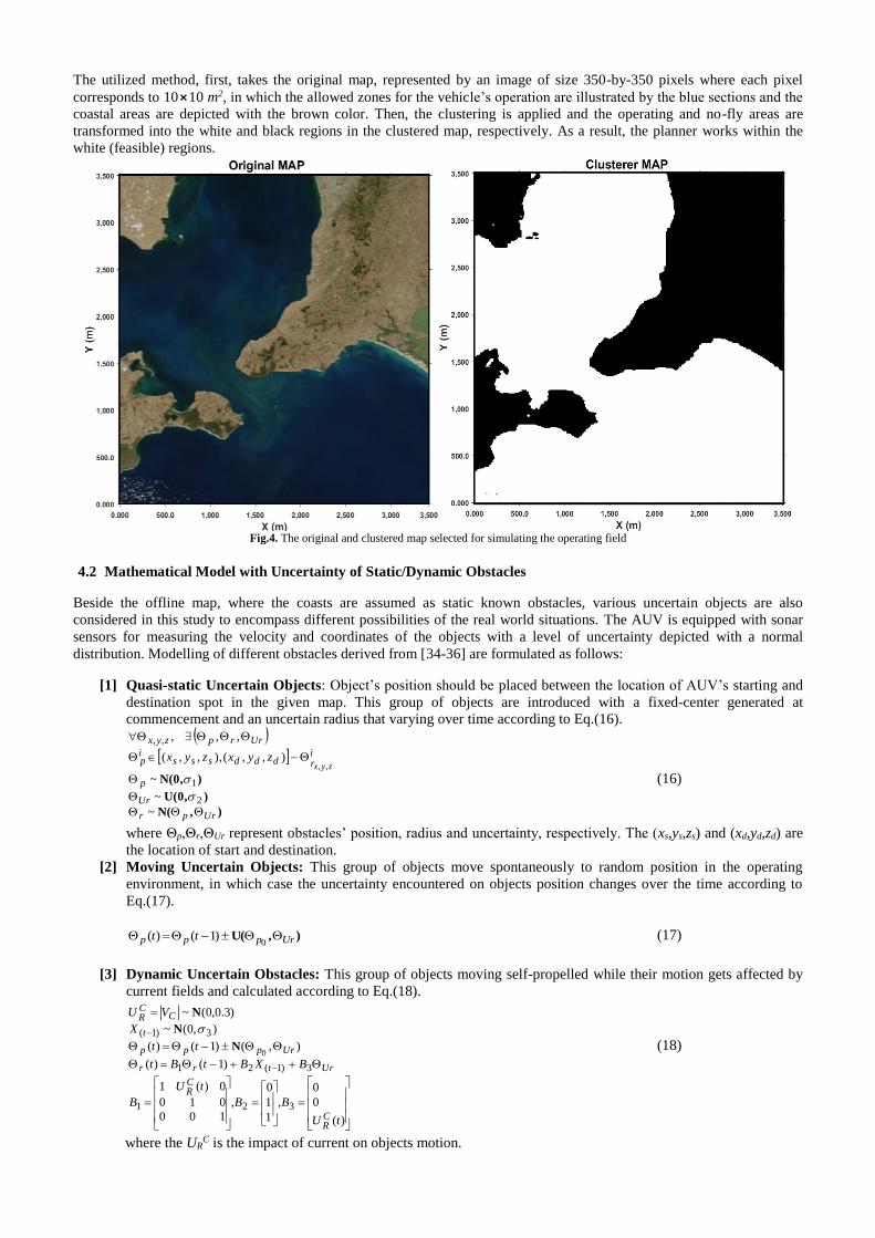
The utilized method, first, takes the original map, represented by an image of size 350-by-350 pixels where each pixel
corresponds to 10⨯10 m2, in which the allowed zones for the vehicle’s operation are illustrated by the blue sections and the
coastal areas are depicted with the brown color. Then, the clustering is applied and the operating and no-fly areas are
transformed into the white and black regions in the clustered map, respectively. As a result, the planner works within the
white (feasible) regions.
Fig.4. The original and clustered map selected for simulating the operating field
4.2 Mathematical Model with Uncertainty of Static/Dynamic Obstacles
Beside the offline map, where the coasts are assumed as static known obstacles, various uncertain objects are also
considered in this study to encompass different possibilities of the real world situations. The AUV is equipped with sonar
sensors for measuring the velocity and coordinates of the objects with a level of uncertainty depicted with a normal
distribution. Modelling of different obstacles derived from [34-36] are formulated as follows:
[1] Quasi-static Uncertain Objects: Object’s position should be placed between the location of AUV’s starting and
destination spot in the given map. This group of objects are introduced with a fixed-center generated at
commencement and an uncertain radius that varying over time according to Eq.(16).
),N(
)U(0,
)N(0,
Urpr
Ur
p
irdddsss
ip
Urrpzyx
zyxzyxzyx
~
~
~
),,(),,,(
,,,
2
1
,,
,,
(16)
where Θp,Θr,ΘUr represent obstacles’ position, radius and uncertainty, respectively. The (xs,ys,zs) and (xd,yd,zd) are
the location of start and destination.
[2] Moving Uncertain Objects: This group of objects move spontaneously to random position in the operating
environment, in which case the uncertainty encountered on objects position changes over the time according to
Eq.(17).
),U( Urppp tt 0
)1()( (17)
[3] Dynamic Uncertain Obstacles: This group of objects moving self-propelled while their motion gets affected by
current fields and calculated according to Eq.(18).
)(
0
0
,
1
1
0
,
100
010
0)(1
)1()(
),()1()(
),0(~
)3.0,0(~
321
3)1(21
3)1(
0
tU
BB
tU
B
BXBtBt
tt
X
VU
CR
CR
Urtrr
Urppp
t
CCR
N
N
N
(18)
where the URC is the impact of current on objects motion.

4.3 Mathematical Model of Static/Dynamic Current Field
This study uses a numerical estimator based on multiple Lamb vortices and Navier-Stokes equations [37] for modeling
ocean current behavior in 3D space. Two types of static and dynamic current flow are mentioned in the following.
[1] The AUV’s deployment usually is assumed on horizontal plane, because vertical motions in ocean structure are
generally negligible due to large horizontal scales comparing vertical [37]. Hence, the physical model employed
by the AUV to identify the current velocity field VC=(uc,vc) mathematically described by Eq.(19)-(20):
2
2)(
2π)(
OSS
C
eS
Vt
(19)
2
2
2
2
)(
20
)(
20
1)π(2
)(
1)π(2
)(
O
O
SS
Oc
SS
Oc
eSS
xxSv
eSS
yySu
(20)
where the ν represents the viscosity of the fluid, ω gives the vorticity , ∆ and ∇ are the Laplacian and gradient
operators, respectively; S is a 2D spatial space, So is the center of the vortex, ℓ is the radius of the vortex, and ℑ is
the strength of the vortex.
[2] A 3D turbulent dynamic current field, is estimated by a multiple layer structure based on the generated 2D current.
The currents circulation patterns gradually change with depth. Therefore, to estimate continuous circulation
patterns of each subsequent layer, a recursive application of Gaussian noise is applied to the parameters of 2D
case. A probability density function of the multivariate normal distribution is employed to calculate the vertical
profile wc of the 3D current VC=(uc,vc,wc), which is given by Eq.(21):
0
0,
)π2det(
1)( )(2
)(
wSS
SS
w
c
ow
To
eSw (21)
where λw is a covariance matrix of the vortex radius ℓ. A parameter γ is used to scale the wc from the current
horizontal profile uc and vc due to weak vertical motions of ocean environment. For generating dynamic time
varying ocean current, Gaussian noise can be applied on So,ℑ, and ℓ parameters recursively as defined in Eq.(22):
)(
0,
0
)(,
10
01
,,
321
)1(2)1(1)(
)1(2)1(1)(
)1(3)1(211
tUA
tUAA
XAA
XAA
XAXASAS
SfV
CR
CR
iii
iii
S
iSi
oi
oi
Oc
yx
(22)
where URC(t) is the update rate of current field in time t, and the rest of the unknown parameters in Eq.(22) are
defined based on normal distribution as follows: X Sx(i-1)~N(0,σSx), X Sy
(i-1)~N(0,σSy), Xℓ(i-1)~N(0,σℓ), Xℑ
(i-1)~N(0,σℑ).
The current field continuously updated every 4s during the AUV path planning process.
5 Review of Evolutionary Algorithms For Path Planning
Before going through the brief review of the employed evolutionary algorithms for the proposed rendezvous path planning,
it is noteworthy to mention how they are applied over the optimization problem. As mentioned before, B-Spline curves are
exploited to parameterize the path. The generated path by B-Spline curves captured from a set of control points like ϑ= {ϑ1,
ϑ2,…,ϑi…, ϑn} in the problem space with coordinates of ϑ1:(x1,y1,z1),…, ϑn :(xn,yn,zn), where n is the number of
corresponding control points. Therefore, appropriate location of these control points play a substantial role in determining
the optimal path. The mathematical description of the B-Spline coordinates is given by Eq.(23):
n
iKiiz
n
iKiiy
n
iKiix
tBtZ
tBtY
tBtX
1,)(
1,)(
1,)(
)()(
)()(
)()(
(23)
Where ϑi is an arbitrary control point along the path (℘), Bi,K(t) is the curve’s blending functions, t is the time step, and K is
the smoothness factor. Further mathematical description of B-Spline curves can be found in [38].
In this regard, all control points should be located in a respective search region constraint to a predefined bounds of
βiϑ=[Li
ϑ, Uiϑ] where Li
ϑ and Uiϑ are the is the lower and upper bounds respectively ,that for a control point like ϑi:(xi,yi,zi) in
the Cartesian coordinates are defined as Eq.(24):
],,...,,...,,[
],,...,,...,,[
],,...,,...,,[
],,...,,...,,,[
],,...,,...,,,[
],,...,,...,,,[
21)(
21)(
21)(
11210)(
11210)(
11210)(
niz
niy
nix
niz
niy
nix
zzzzU
yyyyU
xxxxU
zzzzzL
yyyyyL
xxxxxL
(24)
where (x0,y0,z0) and (xn,yn,zn) are the position of the start and target points, respectively . For the purpose of the
initialization in the optimization process in this study, each control point ϑi:(xi,yi,zi) is generated by Eq.(25):
)()(
)()(
)()(
)()()(
)()()(
)()()(
iz
iz
zi
izi
iy
iy
yi
iyi
ix
ix
xi
ixi
LURandLtz
LURandLty
LURandLtx
(25)
where Rand represents a random function. The ultimate goal of the optimization process is to find the best B-spline’s
control points in the problem space to have an optimal path satisfying the proposed augmented objective function Eq.(14).
Application of different metaheuristic methods may result very diverse on a same problem due to specific nature each
problem; hence, accurate selection of the algorithm and proper matching of the algorithms functionalities according to
nature of a particular problem is important issue to be considered, which usually remained unattended in most of the
engineering and robotics frameworks in both theory and practice.
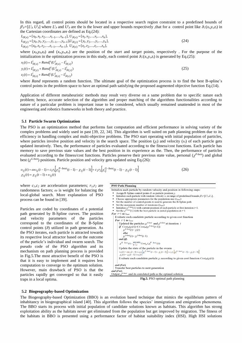
5.1 Particle Swarm Optimization
The PSO is an optimization method that performs fast computation and efficient performance in solving variety of the
complex problems and widely used in past [39, 22, 34]. This algorithm is well suited on path planning problem due to its
efficiency in handling complex and multi-objective problems. The PSO start operating with initial population of particles,
where particles involve position and velocity in the search space. The position (χi) and velocity (υi) of each particle gets
updated iteratively. Then, the performance of particles evaluated according to the fitness/cost functions. Each particle has
memory to save previous state values and the best position in its experience as the. Then, the performance of particles
evaluated according to the fitness/cost functions. Particles preserve their previous state value, personal (χP-best) and global
best (χG-best) positions. Particle position and velocity gets updated using Eq.(26):
)()1()(
)1()1()1()1()1()( 2211
ttt
ttrcttrctt
ijijij
ijbestG
ijijbestP
ijijij
(26)
where c1,c2 are acceleration parameters; r1,r2 are
randomness factors; ω is weight for balancing the
local-global search. More explanation of PSO
process can be found in [39].
Particles are coded by coordinates of a potential
path generated by B-Spline curves. The position
and velocity parameters of the particles
correspond to the coordinates of the B-Spline
control points (ϑ) utilized in path generation. As
the PSO iterates, each particle is attracted towards
its respective local attractor based on the outcome
of the particle’s individual and swarm search. The
pseudo code of the PSO algorithm and its
mechanism on path planning process is provided
in Fig.5.The most attractive benefit of the PSO is
that it is easy to implement and it requires less
computation to converge to the optimum solution.
However, main drawback of PSO is that the
particles rapidly get converged so that it easily
traps in a local optima.
5.2 Biogeography-based Optimization
The Biogeography-based Optimization (BBO) is an evolution based technique that mimics the equilibrium pattern of
inhabitancy in biogeographical island [40]. This algorithm follows the species’ immigration and emigration phenomena.
The BBO starts its process with initial population of candidate solutions known as habitats. This algorithm has strong
exploitation ability as the habitats never get eliminated from the population but get improved by migration. The fitness of
the habitats in BBO is presented using a performance factor of habitat suitability index (HSI). High HSI solutions
Fig.5. PSO optimal path planning

correspond to habitats with more suitable habitation that tend to share their useful information with poor HIS solutions.
There is also a qualitative parameter of Suitability Index Variable (SIV) that is a vector of integers and affects habitability
of solutions. The SIV initialized in advance with random integers. Each candidate solution of habitat (hi) holds migration
parameters of emigration rate (μ), immigration rate (λ), SIV vector; and gets evaluated by its corresponding HIS value
before the BBO start its process. A good solution has a higher rate of μ (emigration) and lower rate of λ (immigration) . The
SIV vector of hi is probabilistically altered according to its immigration rate of λ. In migration process, one of the solutions
(hi) is randomly picked to migrate its SIV to another solution hj regarding its μ value. Then, mutation is exerted to alter the
population and prevent stuck in a local optima. A candidate solution of hi is changed and modified considering probability
of habitance of S species in hi at time t; so its habitance probability at time (t+Δt) is determined using Eq.(28) by holding
one of the conditions given by Eq.(27) as follows:
1:)(:)(
1:)(:)(
:)(:)(
)(,μ,λ)(
StthSth
StthSth
StthSth
tPth
ii
ii
ii
SSSi
(27)
E
S
SE
S
SI
tPtP
tttPttP
SSIEif
S
S
SSSS
SSSS
μλ;
*μ
1*λ
ΔμΔλ
)ΔμΔλ1)(()Δ(
max
max
1111 (28)
where E and I are the maximum emigration and immigration
rates, respectively. Smax is the maximum number of species in
a habitat. Assuming a very small Δt≈0, the Ps is calculated by
Eq.(29).
max11
max1111
11
μ)μ(λ
11λμ)μ(λ
0λ)μ(λ
SSPP
SSPPP
SPP
P
SSSSS
SSSSSSS
SSSSS
S (29)
Solutions with smaller Ps need to be mutated, while habitats
with higher Ps is less likely to mutate; thus, in BBO process,
the mutation rate of m(S) has inverse relation to habitats Ps
value as indicated by Eq.(30).
m ax
m ax
1)(
P
PmSm S
(30)
In Eq.(30), the Pmax is probability of the habitat with Smax and
mmax represents the maximum mutation rate. Further details
can be found in [35].
In the proposed BBO based path planner, each habitat hi
corresponds to the coordinates of the B-Spline control
point’s ϑi utilized in path generation, where hi defined as a
parameter to be optimized (Ps:(h1,h2,…,hn-1)). Habitats get
improved iteratively. The pseudo code of the BBO on path
planning process is provided in Fig.6.
5.3 Firefly Algorithm
Firefly Algorithm (FA) is a kind of meta-heuristic algorithm
[41] captured by sampling the flashing patterns of fireflies.
In the FA process, the fireflies are attracted to each other
according to their brightness, which it gets faded when
fireflies’ distance is increased. The brighter fireflies’ attract
the others in the population. The firefly’s attraction depends
on their distance L and received brightness from the adjacent
fireflies; thus, the firefly χi approaches the χj according to
their attraction parameter β that is calculated by Eq.(31):
)1,0(,
]2
1[)(
0
01
02
2
1
2,,
tt
ti
tj
Lti
ti
L
xxL
randeß
eßß
ij
d
qqjqiijij
(31)
Fig.6. BBO optimal path planning
Fig.7. Pseudo-code of FA mechanism on path planning approach and
encoding scheme based on the path control points

In Eq.(31), the coordinate firefly χi in d dimension space contains q components of 𝑥𝑖,q. The β0 is attraction value of firefly
χi when L=0. The αt and α0 are the randomization factor and initial randomness scaling value, respectively. The γ and δ are
light absorption coefficient and damping factor, respectively. It is noteworthy to mention that there should be a suitable
balance between mentioned parameters because in a case that γ→0 the algorithm mechanism turns to particle swarm
optimization, while β0→0 turns the movement of fireflies to a simple random walk [41]. In path planning procedure, the
fireflies correspond to B-Spline control points ({χ1=ϑ1x,y,z , …, χi=ϑi
x,y,z,…, χn=ϑnx,y,z }) tends to be optimized toward the
best solution in the search space . The FA is more efficient comparing others as it is privileged to apply an automatic
subdivision approach that improves its capabilities in dealing with highly nonlinear and multi-objective problems [42]. The
attraction has inverse relation with distance; therefore, the firefly population gets subdivided and subgroups swarm locally
in parallel toward the global optima, which this mechanism enhances convergence rate of the algorithm. The pseudo-code
of FA based path planning process is provided by Fig.7.
5.4 Differential Evolution
Differential Evolution (DE) algorithm is a population-based optimization algorithm that introduced as a modified version
of genetic algorithm and applies similar evolution operators (crossover, mutation and selection) [43]. DE uses floating
numbers and real coding for presenting problem parameters that enhances solution quality and provides faster optimization.
The algorithm uses a non-uniform crossover and differential mutation; the uses selection operator to propel the solutions
toward the optimum area in the search space. The mechanism of the DE algorithm is given below:
[1] Initialization: In this step the population initialized with solution vectors χi, (i=1,…, imax), in which any vector χix,y,z
is assigned with an arbitrary path ℘ix,y,z while the control points ϑ correspond to elements of χi
x,y,z vector as given by
Eq.(32):
)(),(),(,,
},...,1{
},...,1{
,,,,
max
max
ttt
tt
ii
iz
iy
ix
zti
yti
xtiti
(32)
where imax is the population size, and tmax is the maximum number of iterations.
[2] Mutation: The main reason for superior performance of DE comparing to GA is using an efficacious mutation
scheme. Three solution vector like χr1,t, χr2,t, and χr3,t are picked randomly in iteration t and the difference vector
between them utilized in mutation procedure as given by Eq.(33). This kind of mutation uses a donor parameter,
which donor is one of the randomly selected triplet and accelerates rate of convergence, given by Eq.(34):
]1,0[,321
},...,1{3,2,1
)(
max
,2,1,3,
Firrr
irrr
S trtrftrti
(33)
Grii
jj
idonor ,
3
13
1
(34)
where χ˙i,t and χi,t are mutant and parent solution vector,
respectively. Sf is a scaling factor that balances the
difference vector (χr1,t−χr2,t) and higher Sf enhances
algorithm’s exploration capability. λj ∈[0,1] is a
uniformly distributed parameter.
[3] Crossover: This operator shuffles the mutant
individuals and the existing population members using
Eq.(35):
],1[;,...,1
),...,(
),...,(
),...,(
max
,,
,,,,
,,,,1,
,,,,1,
,,,,1,
innj
kjrrand
kjrrand
xx
xx
xx
Cjtij
Cjtijtij
tintiti
tintiti
tintiti
(35)
where χ¨i,t is the produced offspring and rC ∈ [0,1] is
the crossover rate.
[4] Validation and Selection: The solutions produced by
the mutation and crossover get evaluated and the best
solutions are shifted to the next generation (t+1). All
solutions are evaluated by predefined cost function and
the worst solutions get discarded from the population.
The selection procedure is given by Eq.(36) and the
Fig.8. Pseudo code of DE based path planning

process of DE to the proposed path planning problem is expressed by Fig.8.
)()(
)()(
)()(
)()(
,,,
,,,1,
,,,
,,,1,
tititi
titititi
tititi
titititi
CostCost
CostCost
CostCost
CostCost
(36)
6 Simulation Results and Discussion
There is a significant distinction between theoretical understanding of evolutionary algorithms and their properness for
applying on different problems due to the size, complexity, and nature of different problems. This may lead to different
results using different algorithms, for a same problem. Therefore, careful selection of evolutionary method is of significant
importance. In this part, the simulation results obtained for the rendezvous path planning problem through different
scenarios are shown and analyzed. The objective is to show the performance of the utilized evolutionary methods for
applying to the online path planning mechanism resulting in an adaptive maneuverability of the vehicle in a fully cluttered
dynamic operating field. In each scenario, important aspects of uncertain and cluttered operating field are considered and
the outcome of the planner module is demonstrated. In the last scenario, all possible challenges of a realistic operating field
are implemented and full details of the planner outputs including the generated path, corresponding states’ history and final
rendezvous time, are presented. In the following, first, we describe the configuration of the utilized methods for the
proposed problem and then we introduce the adopted scenarios to consider the performance of the evolutionary methods for
online path planning. The parameter configurations of the algorithms are set as follows:
PSO: The PSO is initialized by 100 particles (candidate paths). The expansion-contraction coefficients also set on
2.0 to 2.5. The inertia weight varies from 1.4 to 0.5.
BBO: The habitats population (imax) is set on 100. The number of kept habitats is set on 40, number of new
habitats is set on 40. The emigration rate is generated by a vector of μ including imax elements in (0,1), and the
immigration rate is defined as λ=1- μ. The maximum mutation rate is set on 0.1.
FA: Fireflies population set on 100, the attraction coefficient base value β0 is set on 2, light absorption coefficient
γ is assigned with 1. The damping factor of δ is assigned with 0.95 to 0.97. The scaling variations is defined based
on initial randomness scaling factor of α0. The parameter of randomization is set on 0.4.
DE: Population size is set on 100, lower and upper bound of scaling factor is set on 0.2 and 0.8, respectively. The
crossover probability fixed on 20 percent.
Meanwhile, the maximum number of iteration for all algorithms is set on tmax=100 and for having stable results the number
of 30 runs for each scenario is applied. Finally, number of control points for each B-Spline path is set on 7.
Scenario 1: Path planning in spatiotemporal ocean flows
To investigate the performance of the proposed online path planning strategy, the ocean environment is modelled as a three
dimensional volume Γ3D covered by uncertain static /moving obstacles and time varying ocean current, as mentioned in
section 4. The update of operating field includes changes in the position of the obstacles or current behaviour, continuously
measured from the on-board sonar and horizontal acoustic Doppler current profiler (HADCP) sensors. Fig.9 represents the
performance of the path planners in adapting ocean currents that varies within 4 time steps (various updating rate) once the
AUV starts to travel from a waypoint on a loitering pattern (shown with a red circle) toward the rendezvous position
(indicated by a yellow square). In this scenario, the variability of the current field is illustrated through four subplots in
Fig.9 labelled by Time Step 1-4. The current field used in Fig.9 is computed from a random distribution of 50Lamb
vortices in a 350×350 grid within a 2D spatial domain according to the pixel size of the clustered map. In order to change
the current parameters, Gaussian noise, in a range of 0.1~0.8, is randomly applied to update current parameters of Sio, ℓ,
and ℑ given in Eq.(19)-(22).
Referring to Fig.9, it is apparent that the generated path by the evolutionary algorithms between the starting point (red
circle) and the final rendezvous position (yellow square) adapts the behaviour of current in all time steps. As can be seen in
each mentioned subplot, by changing the current map, the new information of spatiotemporal current flow, collected by
HADCP, is fed to the online path planner module, and having a certain level of autonomy and adaptation, it generates a
refined path that can avoid severely adverse current flows and can take advantage of favourable ones to speed up the
vehicle motion and nose dive the energy expenditure. Being more specific in comparing the generated paths, obviously the
FA method shows better performance in making use of favourable current flows, comparing to the others. In the second
rank, the path generated by BBO shows significant flexibility in coping with current change specifically when the current
magnitude gets sharper (more clear in turbulent given in Time Step: 3). Fig.10 demonstrates the variation of fitness value
and the rate of solution convergence for the all evolutionary methods through this scenario. As can be seen, the
convergence rate of the PSO is to somehow moderate and the rest of three methods are roughly identical in finding the
optimal solution.

It is noteworthy to mention that setting lower rate for
Gaussian noise parameter (i.e., in range of 0.1 to 0.8)
applied to the current vector field parameters, leads better
fitness values for the generated paths by the all four
algorithms. Moreover, by setting higher current update
rate (where Gaussian noise parameters get greater value
than 0.8), the path fitness value reduces and practically
other conditions remaining constant in path execution
process. Thus, in a dynamic path planner, when the
current field updating rate get significantly greater value
than the path updating rate, the probability of path failure
increases remarkably.
Scenario 2: Path planning in a cluttered field with variable current flow and static obstacles
In this scenario, the operating field is cluttered with the static obstacles, randomly distributed in the problem space. The
variability of the current vector field is the same as the scenario 1. As depicted in Fig.11, distribution of the obstacles is in
such a way that they occupy the solution space, used in scenario 1, for generating the path. In Fig.11(a), the planner module
generates the candidate path considering the underlying current map and obstacles’ situations toward the final rendezvous
position. The current map is updated in the location where the 2Dposition of the vehicle is shown by the yellow triangles;
these changes are obvious in Fig11(b). The thin curves in Fig.11(b) indicate the offline initial paths generated by the
proposed methods (before updating the current map), and the refined paths (online paths), are clearly shown by the thick
curves in Fig.11(c). The utilized FA, BBO, PSO and DE path planning methods are capable of generating a collision free
path against the distribution of obstacles. Here again, the re-planning procedure is helpful to refine the offline path that may
have not been tailored for the vehicle operation in the variable ocean flows. Fig.12 indicates the performance of the
proposed methods in finding the optimal solution considering the augmented objective function in Eq.(14).
Fig.9. Adaptive path behaviour to current updates in 4 time steps
Fig.10. Variation of path cost and violation along the rendezvous mission

As can be seen in Fig.12, the initial solutions generated by
the evolutionary methods are different, as a result of
different natures and mechanisms. However, they all are
capable of searching the optimization space and converge
to the best possible minima. Refereeing to collision
violation plot, it can be inferred that applying the re-
planning strategy around 20th iteration, the violation value
decreases to a great extent and at the end there is no
violation over the obtained solution.
Fig.12. Variation of path cost and collision violation along the rendezvous
mission
Scenario 3: Path planning in a cluttered field with
variable current flow static uncertain /moving obstacles
This scenario becomes more challenging as we add the
uncertain static and moving obstacles to the variable
spatiotemporal current field. The collision boundaries
represented as green spheres around the obstacles
computed with radius Θr~2σo indicating a confidence of
98% that the obstacle is located within this area , referring
to the equations mentioned in section 4. The proposed
obstacles in this scenario are generated with random
position by the mean and variance of their uncertainty
distribution and velocity proportional to current velocity.
The uncertainty over the both static and moving obstacles
are linearly propagated relative to the updating time and
leads to the radius growth of the static obstacles and
simultaneous position and radius changes in the moving
obstacles. As mentioned before, by using on-board sonar
sensors the aforementioned variations of the obstacles are
measured and tracked. Fig.13 illustrates 3D-path generated
by the evolutionary methods for the scenario at hand. In
this figure, for having a clear visualization, just the final
refined path is indicated. As can be seen in this figure, due
to the linear propagation of the uncertainty with time, there
exist a collision boundary encircling the objects. The safe
trajectory is achieved if the vehicle manoeuvre does not
have any intersection with the proposed obstacle boundary.
Obviously enough, the utilized evolutionary path planners
are able to generate a collision free path through the
dynamic obstacles that can satisfy the conditions of the
proposed rendezvous problem. This fact is indicated by
Fig.11. Offline path behaviour and re-planning process in accordance with
current and static obstacles

Fig.14 showing the expedient convergence rate of the methods in finding optimal solution and sharp convergence rate of
collision violation, as iteration goes on.
Fig.13. Evolution curves of FA, DE, BBO, and PSO algorithms with four time step change in water current flow in three-dimension space
Fig.14. Variation of path cost and collision violation along the rendezvous mission
Scenario 4: Path planning in a highly uncertain realistic operating field
In the last scenario, the goal is to thoroughly simulate a highly uncertain cluttered realistic operating field including all
possible barriers to assess the performance of the online path planner considering the rendezvous problem. In this scenario,
the clustered map is used as an underlying environment embodied with variable ocean flows, uncertain static and moving
obstacles. The coastal areas on the map are treated as no-fly zones and the planner should be aware of them. These zones in
a context of an offline obstacles are fed to the planner module before starting the rendezvous mission. The leader AUV
transmits its position, indicated by a yellow square in Fig.15, and the possible rendezvous time that is Tr=1800 (sec) in this
scenario, to the follower counterpart. The threshold of ε=300 (sec) is permitted for the final rendezvous, as mentioned in
(13). The follower AUV water-reference velocity is set on υ=2.5 (m/s) and by which it starts the rendezvous mission from
the red circle indicated on Fig.15. For the current flow, the vortexes radius (ℓ) and strength parameters (ℑ) have been set on
as 2.8 m and 12 m/s, respectively [27]; the uncertain static and moving obstacles follows the same concept used in the
previous scenario. Fig.15 (Time Step: 1) shows the firs path generated by the evolutionary methods. The yellow triangles
indicate the place where the current vector field is updated and the planner uses the new situational awareness of the
environment to refine the previous path. It is noteworthy to mention that the path generated by DE, indicated by red dash
line, does not have collision with the neighbour coast at the start of the mission although in 2D illustration this may seem.
The uncertainty of the obstacles can be clearly seen in the subsequent Time Step: 2-4 of Fig.15. It is obvious form Fig.15
that by severing the complexity of the problem, all the evolutionary path planners still generate safe collision free paths
satisfying the conditions of the proposed NOCP. For example, Fig.16 demonstrates the final mission time achieved by the
evolutionary path planners used in this study. As can be seen, the final time is different stemming from the inherent
differences in structure and mechanism of the proposed methods; however, all of them properly satisfy the assigned
rendezvous time threshold (ε=300 (sec)). The associated variations of the performance index and collision violation per
iteration are depicted in Fig.17. Again, the convergence rate of collision violation to zero is sharp due to the nature of
online planning strategy. Finally, Fig.18 illustrates the history of the states with respect to the vehicular constraints. As can
obviously be inferred, the generated path by the all methods respect the physical constraints over the states and generates
smooth trajectory that is applicable for the vehicle low-level auto pilot module.

Fig.15. The path behaviour and re-planning process in a more complex scenario encountering different uncertain dynamic and static obstacles and current
update in 4 time steps.
Fig.16. Performance of the algorithms for time optimality criterion
Fig.17. Cost and collision violation variations for FA, DE, BBO, and PSO
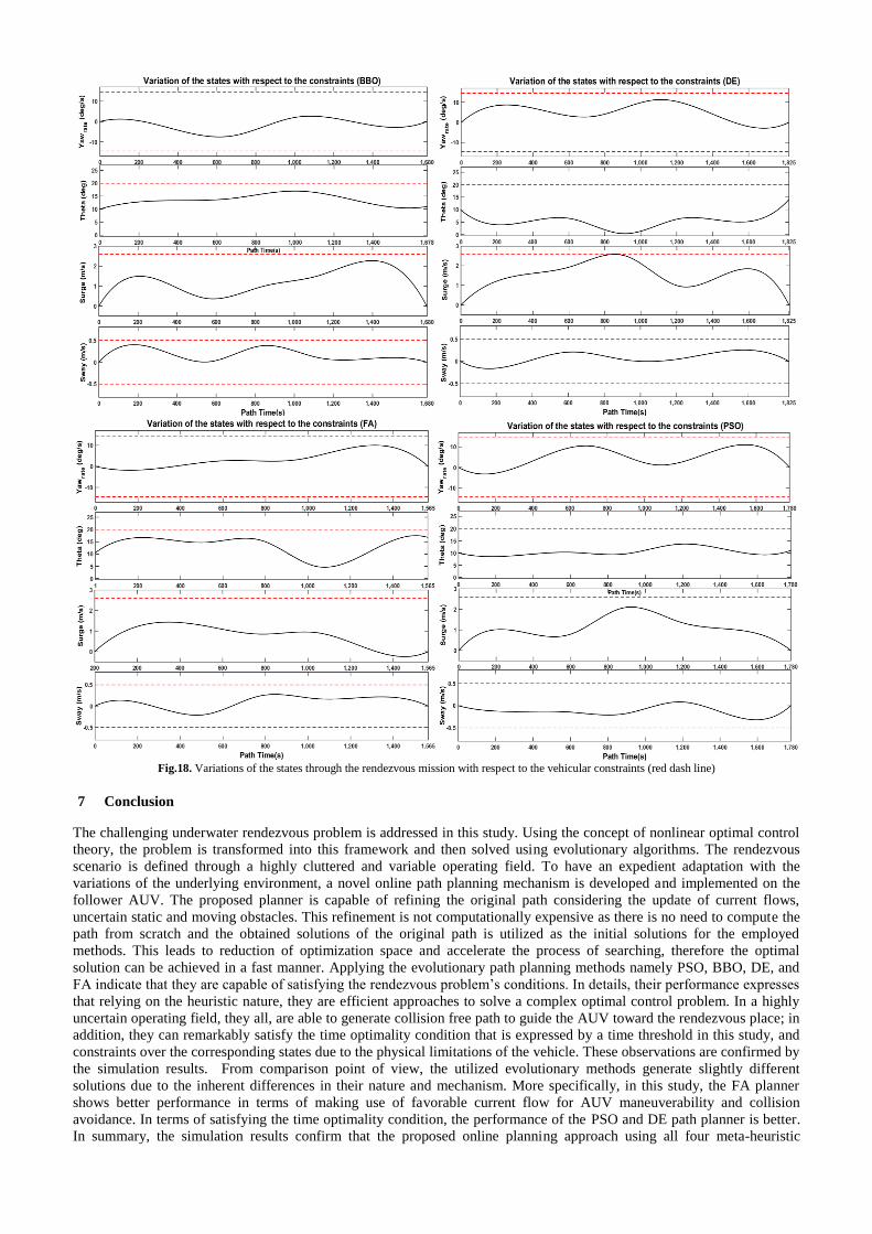
Fig.18. Variations of the states through the rendezvous mission with respect to the vehicular constraints (red dash line)
7 Conclusion
The challenging underwater rendezvous problem is addressed in this study. Using the concept of nonlinear optimal control
theory, the problem is transformed into this framework and then solved using evolutionary algorithms. The rendezvous
scenario is defined through a highly cluttered and variable operating field. To have an expedient adaptation with the
variations of the underlying environment, a novel online path planning mechanism is developed and implemented on the
follower AUV. The proposed planner is capable of refining the original path considering the update of current flows,
uncertain static and moving obstacles. This refinement is not computationally expensive as there is no need to compute the
path from scratch and the obtained solutions of the original path is utilized as the initial solutions for the employed
methods. This leads to reduction of optimization space and accelerate the process of searching, therefore the optimal
solution can be achieved in a fast manner. Applying the evolutionary path planning methods namely PSO, BBO, DE, and
FA indicate that they are capable of satisfying the rendezvous problem’s conditions. In details, their performance expresses
that relying on the heuristic nature, they are efficient approaches to solve a complex optimal control problem. In a highly
uncertain operating field, they all, are able to generate collision free path to guide the AUV toward the rendezvous place; in
addition, they can remarkably satisfy the time optimality condition that is expressed by a time threshold in this study, and
constraints over the corresponding states due to the physical limitations of the vehicle. These observations are confirmed by
the simulation results. From comparison point of view, the utilized evolutionary methods generate slightly different
solutions due to the inherent differences in their nature and mechanism. More specifically, in this study, the FA planner
shows better performance in terms of making use of favorable current flow for AUV maneuverability and collision
avoidance. In terms of satisfying the time optimality condition, the performance of the PSO and DE path planner is better.
In summary, the simulation results confirm that the proposed online planning approach using all four meta-heuristic

algorithms are efficient and fast enough in generating optimal and collision-free path encountering dynamicity of the
uncertain operating field and results in leveraging the autonomy of the vehicle for having a successful mission. For future
researches, internal situations and vehicles fault tolerance also will be encountered to increase vehicle total situational
awareness for establishing more complete robust decision making module and implementing the proposed approach for a
real field trial test.
References
[1] O.A. Yakimenko, D.P. Horner, D.G. Pratt, AUV Rendezvous Trajectories Generation for Underwater Recovery, 16th Mediterranean Conference on Control and Automation. (2008) 1192-1197.
[2] Z. Zeng, A. Lammas, K. Sammut, F. He, Y. Tang, Q. Ji, Path planning for rendezvous of multiple AUVs operating in a variable ocean, IEEE 4th
Annual International Conference on Cyber Technology in Automation, Control, and Intelligent Systems. (2014) 451-456. [3] A.M. Yazdani, K. Sammut, A. Lammas, Y. Tang, Real-time Quasi-Optimal Trajectory Planning for Autonomous Underwater Docking, IEEE
International Symposium on Robotics and Intelligent Sensors. (2015) 15-20. [4] Z. Zeng, L. Lian, K. Sammut, F. He, Y. Tang, A. Lammas, A survey on path planning for persistent autonomy of autonomous underwater vehicles,
Ocean Engineering. (2015), 110, 303-313.
[5] A. M. Galea, Various methods for obtaining the optimal path for a glider vehicle in shallow water and high currents. 11th International Symposium on Unmanned Untethered Submersible Technology. (1999) 150-161.
[6] C. Tam, R. Bucknall, A. Greig, Review of collision avoidance and path planning methods for ships in close range encounters. J. Navig. (2009),
62,455–476. [7] D. Kruger, R. Stolkin, A. Blum, J. Briganti, Optimal AUV path planning for extended missions in complex, fast flowing estuarine environments,
IEEE International Conference on Robotics and Automation, Rom, Italy. (2007) 4265-4270. Doi: 10.1109/ROBOT.2007.364135.
[8] M. Soulignac, Feasible and Optimal Path Planning in Strong Current Fields, IEEE Transactions on Robotics. (2011), 27(1), 89-98. [9] T. Lolla, M.P. Ueckermann, K. Yi|git, P.J. HaleyJr, P.F.J. Lermusiaux, Path planning in time dependent flow fields using level set methods. IEEE
International Conference on Robotics and Automation. (2012) 166-173.
[10] E.W. Dijkstra, A note on two problems in connexion with graphs, Numerische Mathematik, (1959), 1, 269–271. [11] M. Likhachev, D. Ferguson, G. Gordon, A. Stentz, S. Thrun, Anytime dynamic a*: An anytime, replanning algorithm, 15th International
Conference on Automated Planning and Scheduling (ICAPS 2005). (2005) 262–271.
[12] J. Carsten, D. Ferguson, A. Stentz, 3D field D*: improved path planning and replanning in three dimensions. IEEE International Conference on Intelligent Robots and Systems. (2006) 3381-3386.
[13] E. Fernandez-Perdomo, J. Cabrera-Gamez, D. Hernandez-Sosa, J. Isern- Gonzalez, A.C. Dominguez-Brito, A. Redondo, J. Coca, A.G. Ramos, E.A.l.
Fanjul, M. Garcia, Path planning for gliders using regional ocean models: application of Pinzon path planner with the ESEOAT model and the RU27 trans-Atlantic flight data, Oceans’10 IEEE, Sydney, Australia. (2010).
[14] A.A. Pereira, J. Binney, B.H. Jones, M. Ragan, G.S. Sukhatme, Toward risk aware mission planning for autonomous underwater vehicles, IEEE/RSJ
International Conference on Intelligent Robots and Systems, IROS, San Francisco, CA, USA, (2011). [15] C. Petres, Y. Pailhas, J. Evans, Y. Petillot, and D. Lane, Underwater path planning using fast marching algorithms, Oceans Eur. Conf., Brest, France,
Jun. (2005), 2, 814–819.
[16] C. Petres, Y. Pailhas, P. Patron, Y. Petillot, J. Evans, D. Lane, Path planning for autonomous underwater vehicles, IEEE Trans. Robotics. 23(2) (2007).
[17] N.K. Yilmaz, C. Evangelinos, P.F.J. Lermusiaux, N.M. Patrikalakis, Path planning of autonomous underwater vehicles for adaptive sampling using
mixed integer linear programming, IEEE Journal of Oceanic Engineering. (2008), 33(4), 522–537.
[18] S. MahmoudZadeh, D.M.W. Powers, A.M. Yazdani, A Novel Efficient Task-Assign Route Planning Method for AUV Guidance in a Dynamic
Cluttered Environment, Robotics (cs.RO), (2016). arXiv:1604.02524
[19] V. Roberge, M. Tarbouchi, G. Labonte, Comparison of Parallel Genetic Algorithm and Particle Swarm Optimization for Real-Time UAV Path Planning, IEEE Trans. Ind. Inform. (2013), 9(1), 132–141. Doi: 10.1109/TII.2012.2198665.
[20] S. Mahmoudzadeh, D. Powers, K. Sammut, A. Lammas, A.M. Yazdani, Optimal Route Planning with Prioritized Task Scheduling for AUV
Missions, IEEE International Symposium on Robotics and Intelligent Sensors. (2015) 7-15. [21] A. Alvarez, A. Caiti, R. Onken, Evolutionary path planning for autonomous underwater vehicles in a variable ocean, IEEE J. Ocean. Eng. (2004),
29(2), 418–429. Doi:10.1109/joe.2004.827837
[22] J. Witt, M. Dunbabin, Go with the flow: Optimal AUV path planning in coastal environments. In: Proceedings of the 2008 Australasian Conference on Robotics and Automation, ACRA. (2008).
[23] A. Zamuda, J. Daniel Hernandez Sosa, Differential evolution and underwater glider path planning applied to the short-term opportunistic sampling
of dynamic mesoscale ocean structures. Applied Soft Computing , (2014) 24, 95–108. [24] S. MahmoudZadeh, D.M.W. Powers, K. Sammut, A. Yazdani. Differential Evolution for Efficient AUV Path Planning in Time Variant Uncertain
Underwater Environment. Robotics (cs.RO). (2016). arXiv:1604.02523
[25] Y. Fu, M. Ding, C. Zhou, Phase angle-encoded and quantum-behaved particle swarm optimization applied to three-dimensional route planning for UAV, IEEE Trans. Syst., Man, Cybern. A, Syst., Humans. (2012), 42(2), 511–526. doi:10.1109/tsmca.2011.2159586.
[26] Z. Zeng, A.Lammas, K.Sammut, F.He, Y.Tang, Shell space decomposition based path planning for AUVs operating in a variable environment,
Ocean Engineering. (2014), 91, 181-195. [27] Z. Zeng, K. Sammut, A. Lammas, F. He, Y. Tang, Efficient path re-planning for AUVs operating in spatiotemporal currents, Journal of Intelligent &
Robotic Systems. (2014), 79(1),135-153.
[28] B. Garau, M. Bonet, A. Alvarez, S. Ruiz, A. Pascual, Path planning for autonomous underwater vehicles in realistic oceanic current fields: Application to gliders in the Western Mediterranean sea, J.Marit. Res. (2009), 6(2), 5–21.
[29] R.N. Smith, A. Pereira, Y. Chao, P.P. Li, D.A. Caron, B.H. Jones, G.S. Sukhatme, Autonomous underwater vehicle trajectory design coupled with predictive ocean models: A case study, IEEE International Conference on Robotics and Automation. (2010) 4770–4777.
[30] G.A. Hollinger, A.A. Pereira, G.S. Sukhatme, Learning uncertainty models for reliable operation of Autonomous Underwater Vehicles, IEEE
International Conference on Robotics and Automation (ICRA), 6-10 May.(2013) 5593–5599. [31] T.I. Fossen, Marine Control Systems: Guidance, Navigation and Control of Ships, Rigs and Underwater Vehicles, Marine Cybernetics Trondheim,
Norway. (2002).S
[32] A. Homaifar, C.X. Qi, S.H. Lai, Constrained Optimization Via Genetic Algorithms, SIMULATION. (1994), 62(4), 242-254. [33] K. Wagstaff, C. Cardie, Constrained K-means Clustering with Background Knowledge, Proceedings of the Eighteenth International Conference on
Machine Learning. (2001) 577–584.
[34] S. MahmoudZadeh, D.M.W. Powers, K. Sammut, A. Yazdani, Toward Efficient Task Assignment and Motion Planning for Large Scale Underwater Mission, Robotics (cs.RO). (2016). arXiv:1604.04854
[35] S. MahmoudZadeh, D.M.W. Powers, K. Sammut, A. Yazdani, Biogeography-Based Combinatorial Strategy for Efficient AUV Motion Planning and
Task-Time Management, Robotics (cs.RO). (2016). arXiv:1604.04851

[36] S. MahmoudZadeh, D.M.W. Powers, K. Sammut, A.M. Yazdani. 2016. A Novel Versatile Architecture for Autonomous Underwater Vehicle's Motion Planning and Task Assignment, Robotics (cs.RO). (2016). arXiv:1604.03308v2
[37] B. Garau, A. Alvarez, G. Oliver, AUV navigation through turbulent ocean environments supported by onboard H-ADCP, IEEE International
Conference on Robotics and Automation, Orlando, Florida – May. (2006).
[38] I.K. Nikolos, K.P. Valavanis, N.C. Tsourveloudis, A.N. Kostaras, Evolutionary Algorithm Based Offline/Online Path Planner for UAV Navigation,
IEEE Transactions on Systems, Man, and Cybernetics, Part B: Cybernetics. (2003), 33(6), 898–912.
[39] J. Kennedy, R.C. Eberhart, Particle swarm optimization, IEEE International Conference on Neural Networks. (1995) 942–1948. [40] D. Simon, Biogeography-based optimization, IEEE Transaction on Evolutionary Computation. (2008), (12), 702–713.
[41] X. Yang, Firefly algorithms for multimodal optimisation, Proc, 5th Symposium on Stochastic Algorithms, Foundations and Applications, (Eds. O.
Watanabe and T. Zeugmann), Lecture Notes in Computer Science. (2009). 5792: 169-178. [42] X. Yang, X. He, Firefly Algorithm: Recent Advances and Applications, Int. J. Swarm Intelligence. (2013), 1(1), 36-50.
[43] K. Price, R. Storn, Differential evolution – A simple evolution strategy for fast optimization, Dr. Dobb’s J. (1997), 22 (4), 18–24.


![Biogeography-Based Combinatorial Strategy for Efficient ... · An A* algorithm is applied by [12] for AUV path planning problem taking variable vehicle speeds into account. In another](https://img.pdfslide.net/doc/110x75/5fc16fea72ea124a840ee611/biogeography-based-combinatorial-strategy-for-efficient-an-a-algorithm-is-applied.jpg)