Embed Size (px)
Citation preview

Online Data, Fixed Effects and the Construction of High-Frequency Price Indexes
Jan de Haana and Rens Hendriksb
23 September 2013
Abstract: Statistics Netherlands has been experimenting with the collection of prices
from online stores through web scraping. This paper explores whether the unweighted
multilateral time-product dummy, or fixed effects, approach is useful for constructing
high-frequency price index numbers from online data. We explain how unmatched (new
and disappearing) items are treated and how the time-product dummy index compares to
two matched-model price indexes: the chained Jevons index and the multilateral GEKS-
Jevons index. We argue that the time-product dummy method is generally preferable to
the chained matched-model Jevons method but tends to produce similar, though perhaps
slightly less volatile, results as the GEKS-Jevons method. Neither of these methods is
suitable for products where quality change is important or where item identifiers, such
as web IDs, frequently change. Some examples are provided using data extracted from
the website of a Dutch online store.
Key words: fixed-effects models, hedonic quality adjustment, multilateral price index number methods, online prices.
JEL Classification: C43, E31.
a Division of Process Development, IT and Methodology, Statistics Netherlands; and OTB, Faculty of
Architecture and the Built Environment, Delft University of Technology.
Correspondence address: Statistics Netherlands, P.O. Box 24500, 2490 HA The Hague, The Netherlands;
email: [email protected]. b Division of Economic and Business Statistics and National Accounts, Statistics Netherlands; email:
The views expressed in this paper are those of the authors and do not necessarily reflect the views of
Statistics Netherlands. The authors would like to thank Frances Krsinich for introducing them into fixed-
effects modelling and estimating time-product dummy and GEKS-Jevons indexes, and Erwin Diewert for
very helpful comments on a preliminary draft.
1
1. Introduction
Over the past couple of years, Statistics Netherlands has been experimenting with the
collection of prices from the Internet through web scraping. Online prices could perhaps
replace part of the prices observed by price collectors for the compilation of the CPI.1
Online prices might also replace data that is currently being collected from the Internet
in a much less efficient way. Apart from efficiency considerations, web scraping has the
advantage that prices can be monitored daily, allowing the estimation of high-frequency
price indexes. In the Billion Prices Project, a research initiative at MIT that uses online
data to study high-frequency price dynamics and inflation, daily price index numbers
have been calculated for several countries around the world, including the Netherlands.2
For an example on Argentina data, see Cavallo (2012).
Importantly, data on quantities purchased cannot be observed via the Internet.
The lack of quantity data is problematic for the construction of price indexes, but the
problem is not new to statistical agencies. Weighting information at the item level is
generally lacking (unless scanner data is available), and so the agencies are forced to
construct unweighted indexes. For each product, the sample of narrowly defined items
is typically kept fixed, at least for some time, and the index is based on matched items
to compare ‘like with like’. When new items are introduced into the sample to replace
disappearing items, quality-adjustments should be carried out in order to measure pure
price change.
The item samples have traditionally been quite small, particularly to keep things
manageable and control costs. A large part of the costs associated with compiling a CPI
stems from price collection at the stores. If web scraping turns out to be successful, the
costs could be reduced substantially, even when observing all items (displayed on the
website) rather than taking small samples. The costs could be further reduced if it were
possible to develop a method, including a computer system, where quality adjustments
are carried out without manual intervention.
Aizcorbe, Corrado and Doms (2003) claim that it is possible to construct quality-
adjusted price indexes without observing any item characteristics. They suggest using a
1 Hoekstra, ten Bosch and Harteveld (2012) describe some first experiences with the use of web scraping
software, which is part of a broader project at Statistics Netherlands on ‘Big Data’ (Daas et al., 2011).
2 The price indexes are currently compiled by PriceStats, a private company; see www. PriceStats.com.

2
regression model which – instead of including characteristics like in a hedonic model –
includes a set of dummy variables indicating the items plus a set of dummy variables
indicating the time periods. But their idea sounds too good to be true. Diewert (2004)
shows that this method produces a matched-model index in the bilateral case. Silver and
Heravi (2005) argue that in the many-period case, the index “will have a tendency to
follow the chained matched-model results.” De Haan and Krsinich (2012), on the other
hand, have found that the time-product dummy method did make a difference in the
many-period case.
The aim of this paper is threefold: to explain why the multi-period or multilateral
time-product dummy index usually differs from its chained matched-model counterpart,
to show that the time-product dummy method does not produce quality-adjusted price
indexes, and to investigate whether this method is useful for estimating high-frequency
price indexes from online data (for goods where quality change is not a major concern).
The rest of the paper is structured as follows.
The time-product dummy method can be interpreted as a special case of the time
dummy hedonic method, so in section 2 the hedonic method will be discussed in some
detail.
Section 3 addresses the relation between the two methods. Essentially, the time-
product dummy method is based on a regression model where the hedonic price effects
are replaced by item-specific fixed effects. This leads to a model where item identifiers
are the only ‘characteristics’ included. An expression for the time-product dummy index
in terms of geometric average prices and average fixed effects is derived.
Section 4 discusses the treatment of unmatched (new and disappearing) items in
the many-period case. It appears that items with a single price observation in the pooled
data set are ignored in the estimation of the time-product dummy index, indicating that
this method does not produce a quality-adjusted price index.
In section 5 we argue that the time-product dummy method generates a special
type of matched-model price index. We compare the time-product dummy method with
an alternative multilateral approach, the GEKS method. The latter method uses all of the
matches in the data by taking an average of all possible bilateral price comparisons – in
our case using matched-model Jevons indexes – where each period serves as the base.
We show that the time-product dummy method and the GEKS-Jevons method basically
aim at the same (matched-model) index number formula.

3
In section 6 we suggest using a rolling window approach to updating the time
series and discuss problems that may arise when using daily online price data, including
the treatment of regular and sales prices. A related issue is whether the compilation of
daily price indexes would be useful.
Section 7 provides some empirical illustrations. Our data set contains daily price
observations extracted from the website of a Dutch online retailer for three products:
women’s T-shirts, men’s watches, and kitchen appliances.
Section 8 summarizes our findings and concludes.
2. Time dummy hedonic indexes
A hedonic model explains the price of a product from its (performance) characteristics.
Though other functional forms are possible, for convenience we will only consider the
log-linear model
tiik
K
kk
tti zp εβδ ++= ∑
=1
ln , (1)
where tip denotes the price of item i in period t; ikz is the (quantity) of characteristic k
for item i and kβ the corresponding parameter; tδ is the intercept; the random errors tiε have an expected value of zero, constant variance and zero covariance.
The parameters kβ in model (1) are constant across time. Pakes (2003) argues
that this is a (too) restrictive assumption,3 but it allows us to estimate the model on the
pooled data of two or more periods, thus increasing efficiency. Suppose we have data
for a particular product at our disposal for periods Tt ,...,1,0= ; the samples of items are
denoted by TSSS ,...,, 10 and the corresponding number of items by TNNN ,...,, 10 . The
estimating equation for the pooled data becomes
tiik
K
kk
T
t
ti
tti zDp εβδδ +++= ∑∑
== 11
0ln , (2)
3 Data permitting, this assumption can be tested. A more flexible method for estimating quality-adjusted
price indexes is hedonic imputation where the characteristics parameters are allowed to change over time
and the model is estimated separately in each time period. Starting from some preferred index number
formula, the ‘missing prices’ are imputed using the predicted prices from the hedonic regressions. For a
comparison of time dummy and imputation approaches, see Silver and Heravi (2007), Diewert, Heravi
and Silver (2009), and de Haan (2010).

4
where the time dummy variable tiD has the value 1 if the observation pertains to period
t and the value 0 otherwise; the time dummy parameters tδ shift the hedonic surface
upwards or downwards as compared with the intercept term 0δ . The method is usually
referred to as the time dummy method.
Suppose equation (2) is estimated by Ordinary Least Squares (OLS) regression,
yielding parameter estimates 0δ̂ , tδ̂ ),...,1( Tt = and kβ̂ ),...,1( Kk = .4 Since changes
in the item characteristics are controlled for, )ˆexp( tδ is an estimator of quality-adjusted
aggregate price change going from the base period 0 to each comparison period t.5 An
explicit expression for )ˆexp( tδ can be derived in the following manner. The predicted
prices of item i in the base period 0 and the comparison periods t are
= ∑=
K
kikki zp
1
00 ˆexp)ˆexp(ˆ βδ ; (3)
= ∑=
K
kikk
tti zp
1
0 ˆexp)ˆexp()ˆexp(ˆ βδδ ; ),...,1( Tt = . (4)
Taking the geometric mean of the predicted prices for all items belonging to the samples 0S and TSS ,...,1 , respectively, yields
= ∑ ∑∏
= ∈∈
K
k Siikk
Si
Ni Nzp
1
001
0
00
0/ˆexp)ˆexp()ˆ( βδ ; (5)
= ∑ ∑∏
= ∈∈
K
k Si
tikk
t
Si
Nti
tt
t
Nzp1
01
/ˆexp)ˆexp()ˆexp()ˆ( βδδ ; ),...,1( Tt = . (6)
Dividing (6) by (5) and some rearranging gives
−=
= ∑∏
∏
∑ ∑
∑ ∑
∏
∏=
∈
∈
= ∈
= ∈
∈
∈K
k
tkkk
Si
Ni
Si
Nti
K
k Si
tikk
K
k Siikk
Si
Ni
Si
Nti
t zz
p
p
Nz
Nz
p
pt
t
t
t
t
1
01
0
1
1
1
0
10
1
)(ˆexp
)ˆ(
)ˆ(
/ˆexp
/ˆexp
)ˆ(
)ˆ(
)ˆexp(
0
0
0
0
0
ββ
βδ , (7)
4 Under the classical assumptions, OLS regression will suffice. However, estimating a time dummy model
by OLS produces an unweighted price index, which is undesirable from an index number point of view.
When quantity or expenditure information at the item level is available, weighted least squares regression
is preferable, even if it introduces some heteroskedasticity, because a weighted index results.
5 The estimator is not unbiased, but the bias is often negligible in practice. For bias correction terms, see
Kennedy (1981) or van Garderen and Shah (2002).

5
where ∑ ∈= 0
00 /Si ikk Nzz and ∑ ∈
= tSi
tik
tk Nzz / are the unweighted sample means of
characteristic k. Due to the inclusion of time dummies and an intercept into the model,
the OLS residuals sum to zero in each period so that ∏ ∏∈ ∈=0 0
00 /10/10 )()ˆ(Si Si
Ni
Ni pp
and ∏ ∏∈ ∈=t t
tt
Si Si
Nti
Nti pp /1/1 )()ˆ( . Expression (7) can therefore be written as
−== ∑∏
∏=
∈
∈K
k
tkkk
Si
Ni
Si
Nti
ttTD zz
p
p
Pt
t
1
01
0
1
0 )(ˆexp
)(
)(
)ˆexp(
0
0
βδ ; ),...,1( Tt = . (8)
The exponential factor in equation (8) adjusts the ratio of geometric mean prices
for any changes in the average characteristics between period t and the base period 0. If tkk zz =0 , then the quality-adjustment factor equals 1 and the index simplifies to the ratio
of geometric mean prices. A specific instance of this condition holds when the samples 0S and tS coincide so that all items are matched. In this case the time dummy index is
equal to the matched-model Jevons price index, and modelling becomes unnecessary.
In equation (2), period 0 serves as the base and a dummy variable for this period
was excluded to identify the model (to prevent perfect multicollinearity). But regression
theory tells us that the kβ̂ are independent of the choice of base period. Hence, the time
dummy index is transitive and can be written as a period-on-period chained index:
−= ∑∏∏
∏=
−
=
∈
−
∈
−
−
K
kkkk
t
Si
Ni
Si
Ni
tTD zz
p
p
P1
1
11
1
1
0 )(ˆexp
)(
)(
1
1
ττ
τ τ
τ
β
τ
τ
τ
τ
; ),...,1( Tt = . (9)
It is easily checked that expressions (9) and (8) are indeed equivalent.
A similar expression is obtained if bilateral time dummy indexes were estimated
on the pooled data for adjacent periods and subsequently chained. The difference would
be that the estimated characteristics parameters are not kept fixed over the entire period
T,...,0 but will differ across the various links of the chain. An often-heard argument for
chaining is that it maximizes the set of matched items and reduces the need for quality
adjustments. However, although the set of matched items typically shrinks in the course
of time, the argument is not relevant here because the structure of the direct multilateral
index is similar to the structure of the chained bilateral index. It is only the difference
between the estimated parameters from the two approaches that matters.
6
3. Time-product dummy indexes
In the time dummy model (1), both the characteristics of an item and the parameters are
assumed constant over time. This implies that their combined effect on the log of price
is also constant over time. If information on item characteristics is not available, it may
be worthwhile to replace the unobservable hedonic effects ∑ =
K
k ikk z1β by item-specific
fixed values iγ . This leads to the fixed-effects model
tii
ttip εγδ ++=ln . (10)
Suppose across the entire period T,...,0 we observe N different items, many of
which may not be available in every time period. The estimating equation for a pooled
regression corresponding to (10) is
ti
N
iii
T
t
ti
tti DDp εγδα +++= ∑∑
−
==
1
11
ln , (11)
where iD is a dummy variable that has the value of 1 if the observation relates to item i
and 0 otherwise. A dummy for an arbitrary item N is not included (so Nγδα += 0 ) in
order to identify the model. The OLS parameter estimates are α̂ , tδ̂ ),...,1( Tt = and iγ̂
)1,...,1( −= Ni . Note that while items with identical characteristics have identical fixed
effects iγ , the estimates iγ̂ will generally differ.6
Model (11) is the intertemporal counterpart of the well-known country-product
dummy model for estimating price indexes across countries.7 Following de Haan and
Krsinich (2012), we refer to (11) as the time-product dummy model. It has been used by
various researchers to estimate price indexes across time, including Aizcorbe, Corrado
and Doms (2003), Ivancic, Fox and Diewert (2009), Krsinich (2011a,b), de Haan and
Krsinich (2012), and Krsinich (2013).8 From a statistical point of view, the time-product
6 It is not possible to include both characteristics and product dummies as the model will not be identified;
the vector of values for any characteristic can be written as a linear combination of the N-1 vectors for the
product dummies and the intercept.
7 The country-product dummy method is due to Summers (1973). Diewert (1999) and Balk (2001) review
the different approaches to international price comparisons.
8 Balk (1980) discusses a weighted version of this model in the context of constructing price indexes for
seasonal goods. Aizcorbe, Corrado and Doms (2003) use OLS to estimate equation (11) whereas the other
authors listed here use expenditure-share weighted least squares. See the Appendix for details of the latter
approach.

7
dummy method is less efficient than the hedonic time dummy method because more
parameters have to be estimated. The time-product dummy method is cost efficient in
that there is no need to collect information on item characteristics.
In order to derive an explicit expression for the time-product dummy index, we
can follow the same steps as in section 2. For 1,...,1 −= Ni , the predicted prices in the
base period 0 and the comparison periods t ),...,1( Tt = are )ˆexp()ˆexp(ˆ 0iip γα= and
)ˆexp()ˆexp()ˆexp(ˆ itt
ip γδα= , respectively, while for Ni = we have )ˆexp(ˆ 0 α=Np and
)ˆexp()ˆexp(ˆ ttNp δα= . By setting 0ˆ =Nγ we can simply write )ˆexp()ˆexp(ˆ 0
iip γα= and
)ˆexp()ˆexp()ˆexp(ˆ itt
ip γδα= for all i. Taking the geometric mean of the predicted prices
across all i yields
= ∑∏
∈∈ 00
0 01
0 /ˆexp)ˆexp()ˆ(Si
iSi
Ni Np γα ; (12)
= ∑∏
∈∈ tt
t
Si
ti
t
Si
Nti Np /ˆexp)ˆexp()ˆexp()ˆ(
1
γδα ; ),...,1( Tt = . (13)
Dividing (13) by (12), some rearranging and using ∏ ∏∈ ∈=0 0
00 /10/10 )()ˆ(Si Si
Ni
Ni pp and
∏ ∏∈ ∈=t t
tt
Si Si
Nti
Nti pp /1/1 )()ˆ( gives for Tt ,...,1=
[ ]t
Si
Ni
Si
Nti
Si
ti
Sii
Si
Ni
Si
Nti
ttTPD
p
p
N
N
p
p
Pt
t
t
t
t
γγγ
γδ ˆˆexp
)(
)(
/ˆexp
/ˆexp
)(
)(
)ˆexp( 01
0
10
10
1
0
0
0
0
0
0
−=
==
∏
∏
∑
∑
∏
∏
∈
∈
∈
∈
∈
∈ , (14)
where ∑ ∈= 0
00 /ˆˆSi i Nγγ and ∑ ∈
= tSi
ti
t N/ˆˆ γγ are the sample means of the estimated
fixed effects, with 0ˆ =Nγ .
An important question is whether the time-product dummy method generates a
quality-adjusted price index, i.e. whether it properly accounts for new and disappearing
items. In other words, apart from random disturbances, does the factor ]ˆˆexp[ 0 tγγ − in
(14) approximate the quality-adjustment factor ])(ˆexp[1
0∑ =−K
k
tkkk zzβ in equation (8)
well? In section 5 we argue that this is not the case9.
9 This could be empirically shown if information on characteristics was available. Unfortunately, data sets
based on web scraping typically do not contain this type of information. Although many websites show
some characteristics, it is often difficult to extract and put them into the required format for use in hedonic
regressions. Also, different websites tend to show different sets of characteristics for a particular product,
making it difficult to attain consistency across online stores.
8
We will first examine what drives the difference between the unweighted time-
product dummy index and the chained matched-model Jevons index. The time-product
dummy method is a special case of the time dummy method, and so the time-product
dummy index (14) can be expressed as a chain index, similar to equation (9):
[ ]ττ
τ τ
τ
γγ
τ
τ
τ
τ
ˆˆexp
)(
)(1
11
1
1
0
1
1
−= −
=
∈
−
∈∏∏
∏
−
−
t
Si
Ni
Si
Ni
tTPD
p
p
P ; ),...,1( Tt = . (15)
In section 4 below, we decompose a single chain link in (15) into the adjacent-period
matched-model Jevons index and two factors representing the effects of new items and
disappearing items.
4. Unmatched items and the time-product dummy index
To analyse the impact of unmatched items, we need some additional notation. Consider
adjacent periods 1−t and t. The total set of items in period 1−t is ttD
ttM
t SSS ,1,11 −−− ∪= ,
where ttMS ,1− denotes the subset of matched items between periods 1−t and t and tt
DS ,1−
the subset of ‘disappearing’ items (which may appear again later). Similarly, the total
set of items in period t is ttN
ttM
t SSS ,1,1 −− ∪= , where ttNS ,1− denotes the subset of ‘new’
items (observed in period t but not in 1−t ). We denote the size of the respective sets by 1−tN , tN , tt
MN ,1− , ttM
tttD NNN ,11,1 −−− −= , and tt
Mttt
N NNN ,1,1 −− −= . A single chain link in
equation (15) for the time-product dummy index can now be decomposed as
[ ]tt
f
Si
Nti
Si
Nti
f
Si
Si
Nti
Si
Nti
N
ti
ti
tTPD
tTPD
ttD
ttM
ttM
ttD
ttD
ttN
ttM
ttM
ttM
ttN
ttN
ttM
p
p
p
p
p
p
P
P γγ ˆˆexp
)(
)(
)(
)(1
1
1
1
1
1
1
1
11,0
0
,1
,1
,1
,1
,1
,1
,1
,1
,1
,1
,1
,1
−
= −
−
∈
−
∈
−
∈
∈
∈−−
−
−
−
−
−
−
−
−
−
−
−
−
∏
∏∏
∏
∏. (16)
The first bracketed factor in (16) shows the ratio of the geometric average period
t prices of the new and matched items, raised to the power of tttN
ttN NNf /,1,1 −− = (i.e., the
fraction of new items), and the second bracketed factor equals the inverse ratio of the
geometric average period 1−t prices of the disappearing and matched items, raised to
9
the power of 1,1,1 / −−− = tttD
ttD NNf (the fraction of disappearing items). The factor with
the average fixed effects can be written as
[ ]
ttD
ttM
ttM
ttD
ttD
ttN
ttM
ttM
ttN
ttN
f
Si
Ni
Si
Ni
f
Si
Ni
Si
Ni
tt
,1
,1
,1
,1
,1
,1
,1
,1
,1
,1
1
1
1
1
1
)]ˆ[exp(
)]ˆ[exp(
)]ˆ[exp(
)]ˆ[exp(
ˆˆexp
−
−
−
−
−
−
−
−
−
−
=−
∏
∏
∏
∏
∈
∈
−
∈
∈−
γ
γ
γ
γγγ . (17)
Substituting (17) into (16) yields a decomposition of the kind we are looking for:
ttD
ttM
ttM
ttD
ttD
ttN
ttM
ttM
ttM
ttN
ttN
ttM
f
Si
N
i
ti
Si
N
i
ti
f
Si
Si
N
i
ti
Si
N
i
ti
N
ti
ti
tTPD
tTPD
p
p
p
p
p
p
P
P
,1
,1
,1
,1
,1
,1
,1
,1
,1
,1
,1
,1
11
11
1
1
1
11,0
0
)ˆexp(
)ˆexp(
)ˆexp(
)ˆexp(
−
−
−
−
−
−
−
−
−
−
−
−
−
∈
−
∈
−
∈
∈
∈−−
=
∏
∏∏
∏
∏
γ
γ
γ
γ. (18)
If the fixed effects approximate the quality differences well, then the ratios )ˆexp(/ itip γ
and )ˆexp(/1i
tip γ− are ‘quality-adjusted prices’, normalized with respect to the base item
N. Expression (18) shows, for example, that new items have an upward effect compared
with the adjacent-period matched-model Jevons index when their geometric average of
(normalized) quality-adjusted prices is higher than that of the matched items. The larger
the fraction ttNf ,1− of new items, the bigger this effect will be.
There is no reason to expect that the effects of the new and disappearing items in
(18) are both equal to 1 or cancel each other out. Take for example clothing. The prices
of most clothing items decline over time, so a chained matched-model index will have a
downward trend. If the time-product dummy method would work well, the unmatched
items are likely to counter this trend since we expect the average quality-adjusted price
of new (disappearing) items to be above (below) the average quality-adjusted price of
the matched items.10 In that case the bracketed factors in (18) tend to be greater than 1
and the resulting index does not necessarily follow the chained Jevons index. 10 Using a U.S. scanner data set, Greenlees and McClelland (2010) show that a chained matched-model
price index for misses’ tops has a strong downward trend, which is eliminated when hedonic regression is
used. A problem with fashion goods such as clothing is that fashion itself may be regarded as a quality-
determining feature, so that part of the price decline could be attributed to deterioration in quality. But
even if they wanted to, statistical agencies are unable to measure fashion effects. Seasonality in itself is
obviously another problem. For different approaches to the treatment of clothing in a CPI, see Consumer
Price Index Manual: Theory and Practice (ILO et al., 2004).

10
Now recall that )ˆexp()ˆexp()ˆexp(ˆ itt
ip γδα= or )]ˆexp()ˆ/[exp(ˆ)ˆexp( ttii p δαγ = ,
and therefore also )]ˆexp()ˆ/[exp(ˆ)ˆexp( 11 −−= ttii p δαγ . Substituting these results into the
first factor and second factor between square brackets of (18), respectively, gives
ttD
ttM
ttM
ttD
ttD
ttN
ttM
ttM
ttM
ttN
ttN
ttM
f
Si
N
ti
ti
Si
N
ti
ti
f
Si
Si
N
ti
ti
Si
N
ti
ti
N
ti
ti
tTPD
tTPD
p
p
p
p
p
p
p
p
p
p
P
P
,1
,1
,1
,1
,1
,1
,1
,1
,1
,1
,1
,1
1
1
1
1
1
1
1
1
1
11,0
0
ˆ
ˆ
ˆ
ˆ
−
−
−
−
−
−
−
−
−
−
−
−
−
∈−
−
∈−
−
∈
∈
∈−−
=
∏
∏∏
∏
∏. (19)
According to (19), new items will have an upward effect when their average regression
residuals are greater than those of the matched items in period t, i.e., when their prices
are on average unusually high. Decomposition (19) is a well-known result. It holds for
any (OLS) multilateral time dummy index and can be directly derived from the fact that
the regression residuals sum to zero in each period.
Equation (19) does clarify the role of items which are observed only once during
the whole period T,...,0 . By definition these are unmatched items. When using hedonic
regression, they affect measured price change, as they should, but when using the time-
product dummy method, they do not. To understand why this is the case, recall that the
OLS regression residuals for all 1−∈ tSi and tSi ∈ sum to zero. Because each item has
its own dummy variable, the residuals also sum to zero per item. Moreover, for items
observed in one period only, there is just a single observation in the data set, implying 11ˆ −− = t
iti pp and t
iti pp =ˆ for some tt
DSi ,1−∈ and ttNSi ,1−∈ .
When only two time periods, 0 and 1, are considered, equation (19) describes the
decomposition of the bilateral time-product dummy index. In this simple case we have 00ˆ ii pp = for all disappearing items and 11ˆ ii pp = for all new items, so the numerators of
both bracketed factors in (19) are then equal to 1. The denominators are also equal to 1
because the residuals for the matched items, which are observed in periods 0 and 1, also
sum to zero in each time period. Thus, the bilateral time-product dummy index equals
the matched-model Jevons price index.
Diewert (2004) has shown this result earlier in the context of two countries.11 He
notes that the method “can deal with situations where say item n* has transactions in
one country but not the other” and that “the prices of item n* will be zeroed out”. The
11 Silver and Heravi (2005) have done the same for two time periods.

11
fact that, while their fixed effects can be estimated, items with a single observation are
zeroed out in the two-period case, carries over to the many-period case. This does not
mean that a chained matched-model Jevons index results, as we have seen. Items which
are ‘new’ or ‘disappearing’ in comparisons of adjacent periods are typically observed
multiple times during T,...,0 and are not zeroed out. They contain information on price
change that is used in a multilateral time-product dummy regression whereas they are
ignored in a chained matched-model index.
5. A comparison with the GEKS-Jevons index
The fixed effects in a time-product dummy model can be seen as item-specific hedonic
price effects, assuming the parameters of the characteristics in the underlying log-linear
hedonic model are constant across time. This leads Aizcorbe, Corrado and Doms (2003)
and Krsinich (2013) to believe that the time-product dummy method produces a quality-
adjusted price index. But measuring quality-adjusted price indexes without information
on item characteristics is just not possible. This is almost trivial from a modelling point
of view. In a hedonic model, the exponentiated time dummy coefficients are estimates
of quality-adjusted price indexes since we control for changes in the characteristics. In
the time-product dummy model, there is nothing to control for as auxiliary information
on characteristics is not included.
The exponentiated time dummy coefficients in the time-product dummy method
do not measure quality-adjusted price change but represent a particular type of matched-
model price change. In this section, we will compare the unweighted multilateral time-
product dummy method to a competing transitive approach, the unweighted multilateral
GEKS method. It will be shown that if a time dummy hedonic model holds true, which
is the basic assumption underlying the time-product dummy method, the two methods
basically aim at the same matched-model index number formula.
The GEKS method was designed for making transitive price comparisons across
countries. Ivancic, Diewert and Fox (2011) have adapted the GEKS method to construct
transitive comparisons across time.12 The GEKS index going from period 0 to period t
),...,0( Tt = can be expressed as 12 For applications on Dutch and New Zealand scanner data, see de Haan and van der Grient (2011) and
de Haan and Krsinich (2012), respectively.

12
( )∏=
+×=T
l
TltltGEKS PPP
0
1
100 , (20)
where lP0 and ltP are bilateral price indexes between periods 0 and l and periods l and
t. Period l ),...,0( Tl = serves as the link period or base period for the various bilateral
comparisons. In its standard form, the GEKS method uses bilateral matched-model price
indexes.
When quantity data is available, as in scanner data, superlative bilateral indexes
such as the Fisher or Törnqvist should be used. If quantity data is lacking, as with online
data, Jevons indexes can be used instead. Superlative as well as Jevons indexes satisfy
the time reversal test, which is a prerequisite for the GEKS method. In this section we
focus on bilateral Jevons indexes, so in (20) we have
∏∈
==
lM
lM
Si
N
i
lil
Jl
p
pPP
0
0
1
000 , (21)
∏∈
==
ltM
ltM
Si
N
li
tilt
Jlt
p
pPP
1
, (22)
where lMS0 and lt
MS denote the matched samples between the respective periods with
sizes lMN 0 and lt
MN . Note that 100 == ttJJ PP , as required. Thus, the GEKS-Jevons13 price
index (20) can be written as
( ) ( ) ( ) ( ) 1
20
1
1
1
1
1
10
1
1
10000 11 +
≠=
+
≠=
+
≠=
+− ∏∏∏ =×××××= Tt
J
T
tll
TltJ
T
tll
TlJ
T
tll
TtJ
tJ
ltJ
lJ
tJGEKS PPPPPPPP , (23)
showing that tJP0 , the bilateral index going directly from period 0 to period t, ‘counts
twice’.
In section 4 we have seen that the price index arising from an unweighted time-
product dummy regression on the pooled data of two periods simplifies to the bilateral
matched-model Jevons price index. This means we can write the bilateral price indexes
(21) and (22) as time-product dummy indexes, which facilitates a comparison with the
multilateral time-product dummy index. That is, in equation (23) we set llTPD
lJ PP 0
),0(0 = ,
lttlTPD
ltJ PP ),(= and t
tTPDt
J PP 0),0(
0 = , where (0,l), (l,t) and (0,t) refer to bilateral comparisons
13 Following Balk (2008), we refer to the GEKS method as the procedure to obtain transitivity, no matter
what type of bilateral index is used, and write “GEKS-Jevons” when bilateral Jevons price indexes enter
the computation.

13
between periods 0 and l, periods l and t, and periods 0 and t. From section 4 it follows
that
[ ]lll
Si
Ni
Si
Nli
llTPD
p
p
Pl
l
),0(0
),0(10
1
0),0( ˆˆexp
)(
)(
0
0
γγ −=
∏
∏
∈
∈ ; (24)
[ ]ttl
ltl
Si
Nli
Si
Nti
lttlTPD
l
l
t
t
p
p
P ),(),(1
1
),( ˆˆexp
)(
)(
γγ −=
∏
∏
∈
∈ ; (25)
[ ]ttt
Si
Ni
Si
Nt
ttTPD
p
p
Pt
t
),0(0
),0(10
1
00
),0( ˆˆexp
)(
)(
0
0
γγ −=
∏
∏
∈
∈ , (26)
where we have ∑ ∈= 0
0),0(
0),0( /ˆˆ
Si lil Nγγ , ∑ ∈= lSi
lli
ll N/ˆˆ ),0(),0( γγ , ∑ ∈
= lSi
ltli
ltl N/ˆˆ ),(),( γγ ,
∑ ∈= tSi
ttli
ttl N/ˆˆ ),(),( γγ , ∑ ∈
= 0
0),0(
0),0( /ˆˆ
Si tit Nγγ and ∑ ∈= tSi
tti
tt N/ˆˆ ),0(),0( γγ . These are
the sample averages of the estimated fixed effects we would find when estimating the
bilateral time-product dummy model by OLS regression on the pooled data of periods 0
and l, l and t, and 0 and t, respectively.
After substituting equations (24), (25) and (26) into (23), we find the following
expression for the GEKS-Jevons index:
[ ]{ } [ ]{ } [ ]{ } 1
2
),0(0
),0(
1
1
1),0(),(
1
1
1),(
0),0(1
0
1
0 ˆˆexpˆˆexpˆˆexp
)(
)(
0
0
++
≠=
+
≠=
∈
∈− −−−= ∏∏
∏
∏Tt
tt
TT
tll
ll
ltl
TT
tll
ttll
Si
Ni
Si
Nti
tJGEKS
p
p
Pt
t
γγγγγγ
2
),0(0
),0(
;1 ;1
),0(),(
;1
),(
;1
0),0(
10
1
1
ˆ
1
ˆexp
1
ˆ
1
ˆexp
1
ˆ
1
ˆexp
)(
)(
0
0
+−
+
+−
+
+−
+= ∑ ∑∑∑
∏
∏≠= ≠=≠=≠=
∈
∈
TTTTTTp
p ttt
T
tll
T
tll
ll
ltl
T
tll
ttl
T
tll
l
Si
Ni
Si
Nti
t
t
γγγγγγ
1
1
;1
),0(),(),0(
;0),(
0),0(
1
0),0(
10
1
1
ˆˆexp
1
ˆˆ
1
ˆˆ
exp
)(
)(
0
0
+−
≠=
≠==
∈
∈
−−
+
+−
+
+= ∑
∑∑
∏
∏ T
T
T
tll
ll
ltl
tt
T
tll
ttlt
T
ll
Si
Ni
Si
Nti
TTTp
pt
t
γγγγγγ. (27)
14
Equation (27) decomposes the GEKS-Jevons price index into three factors. The
first factor is the ratio of geometric mean prices in periods t and 0. The second factor is
the antilog of the difference between the (arithmetic) averages of 0),0(ˆ lγ ),...,1( Tl = and
ttl ),(γ̂ );,...,0( tlTl ≠= , where 0
),0(ˆ tγ and tt ),0(γ̂ count twice. The third factor is the antilog
of the average of ll
ltl ),0(),( ˆˆ γγ − );,...,1( tlTl ≠= , raised to the power of )1/()1( +− TT .
We expect the third factor to be relatively small and fluctuate around zero over time.
The GEKS-Jevons index is therefore most likely driven by the first two factors.
Let us compare decomposition (27) with decomposition (14) for the multilateral
time-product dummy index. tJGEKSP0
− and tTPDP0 are both written as the ratio of geometric
mean prices in periods t and 0, adjusted by factors based on differences in average fixed
effects. The average fixed effects for period 0 and period t in (27), 0),0(ˆ lγ and t
tl ),(γ̂ , can
be viewed as crude approximations of 0γ̂ and tγ̂ in (14) because, by assumption, they
all measure the same average fixed effects, albeit estimated on different subsets of the
data. Thus, the means ∑ =++T
l tl T1
0),0(
0),0( )1/()ˆˆ( γγ and )1/()ˆˆ( 0 ),0(),(∑
≠= ++T
tll
tt
ttl Tγγ are also
approximations of 0γ̂ and tγ̂ , but much more stable than the elements 0),0(ˆ lγ and t
tl ),(γ̂ .
The third factor in (27), which of course does not appear in (14), adds noise to the first
two factors.
This result suggests that the unweighted time-product dummy and GEKS-Jevons
indexes essentially aim at the same index number formula and are likely to have similar
trends. There can be a difference in smoothness, the time-product dummy index perhaps
being a little smoother. Hence, if a time dummy hedonic model describes the data well,
then the time-product dummy method can be viewed as a (smoothed) approximation of
the matched-model GEKS method.
Our finding is not surprising. The only information entering the estimation of the
time-product dummy index is the prices, or price changes, of all items that are observed
more than once, i.e., items that are matched during some periods of the window T,...,0 ,
because the other items are zeroed out. This is the exact same information that is used to
construct the GEKS index. The time-product dummy method imputes ‘missing prices’14,
but the imputations are unlikely to affect the trend as compared with the GEKS method
as long as the underlying assumptions are satisfied.
14 Summers (1973) proposed the country-product dummy method for estimating transitive price indexes
across countries with the aim of obtaining a full set of prices through imputations for products that are
purchased in one country but not in all other countries.

15
When the true characteristics parameters change over time, or if a single model
is too restrictive, the basic assumption underlying the time-product dummy model will
be violated. As the two methods treat the price changes of the matched items differently,
a difference in trend between GEKS and time-product dummy indexes can arise. The
time-product dummy method has a potential practical advantage though: the indexes are
easier to estimate, assuming the statistical package or computer system can handle large
amounts of data and run regressions that include many time and product dummies.
6. Issues with daily online data and daily indexes
A problem with multilateral methods is that when data for the next period ( 1+T in our
case) is added and the model is re-estimated, the results for all previous periods ),...,1( T
change. Statistical agencies do not accept continuous revisions of their price statistics. A
rolling window approach can be used to overcome the revisions problem. For example,
a multilateral time-product dummy hedonic model would be estimated on the data of a
window with a fixed length, in our case of 1+T time periods, which is shifted forward
each time period. The most recent period-on-period index movement is then repeatedly
spliced onto the existing time series.15
A window length of at least one year will be necessary to cope with seasonal
goods. On the other hand, it does not seem very helpful choosing a window length that
exceeds the average period items – as identified by web IDs or article numbers – are
offered for sale. The lifetime will depend on the type of product, the prevailing market
circumstances and the stores’ or manufacturers’ policy of changing item identifiers. The
importance of the latter issue has not always been fully recognized.
For measuring price change, items should ideally be identified by a complete set
of characteristics; items with identical (quantities of) characteristics are deemed similar.
The number of characteristics needed to distinguish between different items can be quite
large, so usual practice is to choose a limited set of important characteristics. If there are
no item descriptions at all, as we have with web scraping data, or in case it would be too
time consuming to identify items uniquely from product descriptions, the only feasible
15 Ivancic, Diewert and Fox (2011) employ a rolling window approach in the context of GEKS-Fisher
price indexes.

16
solution will be to rely on item identifiers found on websites, such as article numbers or
web IDs.
However, these item identifiers may be too detailed for our purpose as different
article numbers or web IDs can relate to items which are similar from the consumers’
point of view.16 Item churn will then be overestimated and matched-model indexes will
be based on fewer matches than desirable. Price changes of items whose article numbers
or web IDs have changed but otherwise remained unchanged are captured by hedonic
regression methods, although the results become increasingly model dependent. But
such hidden price changes will be missed by matched-model methods,17 including the
time-product dummy method.
There are a number of issues that are specific to web scraping data. Online prices
for supermarkets in the Netherlands are usually 5-6% above shelf prices due to delivery
costs. In turn, shelf prices may differ from average transaction prices (i.e. unit values) as
a result of promotional sales and the like. Representativity of the online data is another
issue. The range of products shown on websites need not be the same as offered in the
corresponding (physical) outlets and may change very frequently, even on a daily basis.
Changes made to the website are a potential problem associated with web scraping since
it could lead to missing price observations. Also, for clothing in particular, online stores
sometimes classify items that are on sale in a separate (clearing) sales category, and this
category should not be overlooked.
The last point raises an important issue. It is obvious that both regular and sales
prices should be taken into account for measuring price change, but it is not so obvious
how they should be treated. Suppose first, following the Billion Prices Project at MIT,
that we observe prices on a daily basis and follow the price change over time of each
individual item as long as it is available. While this price trajectory shows the change in
offer prices, the observed price trend is not necessarily the right one from the average
consumer’s perspective as a result of promotional sales. For example, it might happen
16 This issue was also mentioned by Bradley et al. (1997), who investigated the potential uses of scanner
data in the U.S. CPI, and by de Haan (2002).
17 The first step traditionally followed by statistical agencies when an item is replaced by a newly sampled
item is to find out whether or not the items are comparable. If they are, the prices are directly compared
(and if they are not, a quality adjustment should be made); see for example Chapter 17 in the U.S. Bureau
of Labor Statistics Handbook of Methods, available at www.bls.gov. This procedure ensures that hidden
price changes will not be missed.

17
that regular prices stay constant over time but sales prices show an upward trend. Since
promotional sales occur infrequently relative to the number of days with regular prices,
the overall trend seems to be almost flat. However, if consumers mainly buy the item at
times of sales,18 then the change in sales prices would be a better indicator of the change
in prices actually paid.
Partly due to promotional sales, daily price indexes may be quite volatile, at least
at the product level. It is questionable whether users benefit from volatile price indexes,
and they may want to smooth out volatility. Alternatively, the statistical agency could
do ‘internal smoothing’ by constructing price indexes at a lower frequency, for example
weekly or monthly. There is another reason why the construction of daily indexes from
online data may not be very meaningful. Prices of many products, particularly services,
cannot be observed online. For these products, official price indexes are available from
most statistical agencies on a monthly basis only, so it seems that a month is the shortest
period possible to combine official figures with online data to calculate an overall CPI.19
Ideally, monthly unit value indexes are computed at the item level, which would resolve
the sales problem mentioned above. But without information on quantities purchased,
calculating unit values from daily online data is not possible.
In many cases, scanner data is an ideal source for computing unit values, but that
might be different for online purchases, in particular on clothing. Statistics Netherlands
has received a research scanner database from a major Dutch online store. An issue is
the way in which goods that were returned by the customers are treated. The quantities
registered in a particular month refer to quantities delivered minus quantities returned.
This means that quantities can be negative, something we observed in the database for a
number of goods. More generally, it is not immediately clear how quantities purchased
in each month and the corresponding unit values should be determined. This issue needs
more attention.
18 We saw this for a number of products in supermarket scanner data. An illustrative example for the most
popular make of detergents in the Netherlands is shown in de Haan (2008). Quantities sold at the regular
price were negligible.
19 PriceStats uses officially published monthly indexes for unobserved products to calculate daily overall
inflation measures, apparently by assuming that these indexes are constant across the whole month: “Most
of the categories that we are not able to cover are services. This, however, is not a problem for our goal to
detect the main changes in inflation trends. Services are usually quite stable and not the main source of
volatility.” (www.PriceStats.com/faqs)

18
7. Empirical results
In this section we present some empirical results. The main goal is to illustrate that the
different types of price indexes discussed in the paper, i.e. TPD, chained matched-model
Jevons, and GEKS-Jevons indexes, can have quite different trends and are often highly
volatile when constructed at a daily frequency. Our data set contains daily offer prices
extracted from the website of a Dutch online store for three products: women’s T-shirts,
men’s watches, and kitchen appliances. Actually, we exploit two data sets. The first data
set covers the period of 6 October 2012 to 8 April 2013; the sample period is extended
to 12 August 2013 in the second data set.20 Note that this online retailer has no physical
store, and so the data relate to (potential) online purchases only.
Figures 1-3 compare daily time-product dummy (TPD) and chained Jevons price
indexes for the three products (with 6 October 2012 as the base period), based on the
initial small data set. The change in unweighted arithmetic and geometric average prices
is also plotted. As shown by equation (14), the difference between the TPD index and
the ratio of geometric average prices results from differences in the sample means of the
estimated fixed effects. A couple of things are worth mentioning.
For women’s T-shirts (Figure 1), we observe a noticeable difference between the
TPD and chained Jevons indexes, the TPD sitting above the chained Jevons. This is in
accordance with our expectations, as discussed in section 4. Both price indexes appear
to have substantial downward bias, which also meets our expectations because both are
matched-model indexes based on ‘too detailed’ item identifiers and/or a lack of quality
adjustment. The two indexes are very volatile. Due to compositional changes, average
prices are even more volatile. Yet the trend in average prices seems a lot more plausible
as an indicator of aggregate price change than the trend of the TPD index. Although the
sample period is too short to draw any definitive conclusions, a seasonal pattern appears
to emerge with average prices declining in autumn and winter, and then rising again in
spring.
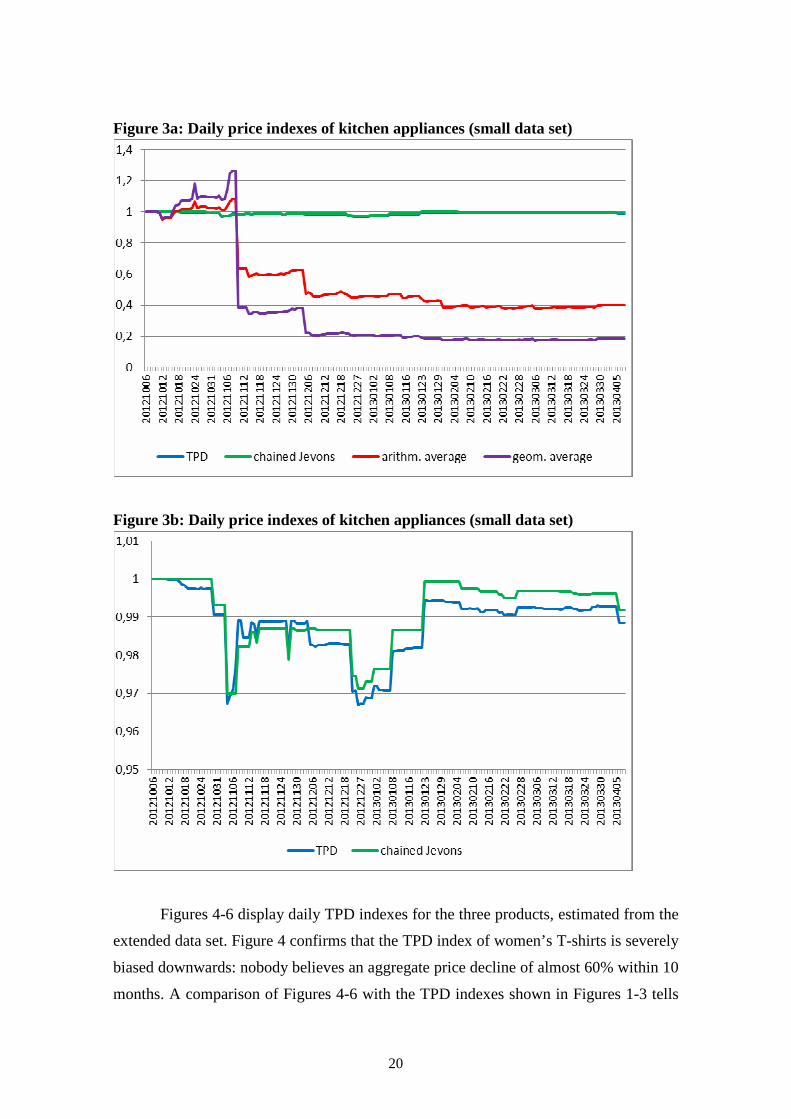
Heterogeneity probably is greater for men’s watches and kitchen appliances than
for women’s T-shirts, which at least partly explains the erratic behaviour of the average
prices (Figures 2 and 3a). The trends of the TPD and chained Jevons indexes for these
20 The price indexes based on the extended data set were kindly estimated by Frances Krsinich (Statistics
New Zealand).

19
products look reasonable. In Figure 3b the left scale has been adjusted in order to show
that the TPD and chained Jevons indexes for kitchen appliances are also volatile, though
much less so than average prices. The differences in volatility as well as in index levels
between the two indexes are minor.
Figure 1: Daily price indexes of women’s T-shirts (small data set)
0,4
0,5
0,6
0,7
0,8
0,9
1
1,1
20
12
10
06
20
12
10
12
20
12
10
18
20
12
10
24
20
12
10
31
20
12
11
06
20
12
11
12
20
12
11
18
20
12
11
24
20
12
11
30
20
12
12
06
20
12
12
12
20
12
12
18
20
12
12
27
20
13
01
02
20
13
01
08
20
13
01
15
20
13
01
21
20
13
01
27
20
13
02
03
20
13
02
09
20
13
02
15
20
13
02
21
20
13
02
27
20
13
03
05
20
13
03
11
20
13
03
17
20
13
03
23
20
13
03
29
20
13
04
04
TPD arithm. average chained Jevons geom. average
Figure 2: Daily price indexes of men’s watches (small data set)
20
Figure 3a: Daily price indexes of kitchen appliances (small data set)
Figure 3b: Daily price indexes of kitchen appliances (small data set)
Figures 4-6 display daily TPD indexes for the three products, estimated from the
extended data set. Figure 4 confirms that the TPD index of women’s T-shirts is severely
biased downwards: nobody believes an aggregate price decline of almost 60% within 10
months. A comparison of Figures 4-6 with the TPD indexes shown in Figures 1-3 tells

21
us that the revisions of index numbers previously estimated from the small data set are
negligible in relation to the volatility of the indexes.
Figure 4: Daily TPD price indexes of women’s T-shirts (large data set)
Figure 5: Daily TPD price indexes of men’s watches (large data set)

22
Figure 6: Daily TPD price indexes of kitchen appliances (large data set)
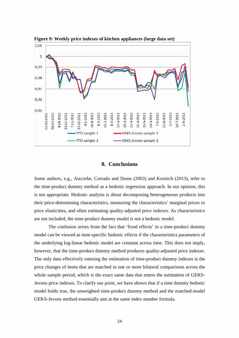
When trying to estimate GEKS-Jevons indexes on the big data set, it turned out
that the SAS program was unable to handle such a large amount of data. We decided to
randomly sample one observation out of seven daily observations per item in each of
the 43 weeks. Two independent samples were drawn to get a better understanding of the
potential effects of sampling in time. Figures 7-9 compare the resulting weekly GEKS-
Jevons price indexes with weekly TPD indexes estimated from the same samples.
For women’s T-shirts (Figure 7), the GEKS-Jevons index does not fall as fast as
the TPD index, which is a bit surprising, but for men’s watches (Figure 8) and kitchen
appliances (Figure 9), the two indexes are very similar. Note that the difference between
the indexes estimated from sample 1 and sample 2 is small for each product. Comparing
Figures 7-9 with Figures 1-2 reveals that drawing samples does not change the picture
much (during 6 October 2012 to 8 April 2013), both in terms of trends and volatility.
Apparently, there is a lot of redundancy in the daily data set. This again raises doubts
about the usefulness of observing prices on a daily basis. For the three products, weekly
web scraping would suffice, unless of course the aim is to explicitly compile daily price
indexes.
The above results are preliminary. In future work we should take a closer look at
the microdata. Previous analysis of web scraping data from another Dutch online store
indicated that many items were missing as a result of day-to-day changes in the website,

23
even though these items were most likely available for purchase. It may be worthwhile
to impute temporarily ‘missing prices’, for example by carrying forward the latest price
observations. In particular, it would be interesting to investigate how imputations affect
the volatility of the daily and weekly time series.
Figure 7: Weekly price indexes of women’s T-shirts (large data set)
Figure 8: Weekly price indexes of men’s watches (large data set)
24
Figure 9: Weekly price indexes of kitchen appliances (large data set)
8. Conclusions
Some authors, e.g., Aizcorbe, Corrado and Doms (2003) and Krsinich (2013), refer to
the time-product dummy method as a hedonic regression approach. In our opinion, this
is not appropriate. Hedonic analysis is about decomposing heterogeneous products into
their price-determining characteristics, measuring the characteristics’ marginal prices or
price elasticities, and often estimating quality-adjusted price indexes. As characteristics
are not included, the time-product dummy model is not a hedonic model.
The confusion arises from the fact that ‘fixed effects’ in a time-product dummy
model can be viewed as item-specific hedonic effects if the characteristics parameters of
the underlying log-linear hedonic model are constant across time. This does not imply,
however, that the time-product dummy method produces quality-adjusted price indexes.
The only data effectively entering the estimation of time-product dummy indexes is the
price changes of items that are matched in one or more bilateral comparisons across the
whole sample period, which is the exact same data that enters the estimation of GEKS-
Jevons price indexes. To clarify our point, we have shown that if a time dummy hedonic
model holds true, the unweighted time-product dummy method and the matched-model
GEKS-Jevons method essentially aim at the same index number formula.

25
Measuring quality-adjusted price change without data on item characteristics is
just not possible. The two multilateral methods should therefore not be applied to goods
where quality change is important.21 De Haan and Krsinich (2012) show how the GEKS
method can be modified to account for quality change by using hedonic rather than
matched-model price indexes as input in the GEKS system.22 For goods where quality
change is of minor importance, the two methods have much to offer as compared to a
period-on-period chained matched-model price index since they use all of the matches
across the whole sample period. We would prefer the GEKS method because it is the
most straightforward way to obtain transitive indexes and because it is a nonparametric
approach whereas the time-product dummy method is model-based. Minimising model
dependence seems like good advice for producing official statistics. The identification
of items remains an issue. Any matched-model method breaks down when changes in
item identifiers and price changes occur simultaneously.
The time-product dummy method has a practical advantage though, in particular
when the aim is to construct high-frequency price index numbers using online data. If
the production system can deal with very large data sets, time-product dummy indexes
may be easier to estimate than GEKS indexes. Also, our equations (18) and (19) provide
practitioners with the opportunity to decompose the latest period-on-period price change
into a matched-model index and the effects of items that are new or disappearing with
respect to the previous period. The latter effects are implicitly based on the data of many
earlier periods. Staff involved in production of the CPI may not like this aspect, but it is
unavoidable with multilateral methods.
21 This is also true for the chained matched-model Jevons method, which is how PriceStats compiles daily
indexes for each product category. On their website (www.PriceStats.com/faqs) it is mentioned that “We
treat all individual products [what we call items] as separate series, without making product substitutions
or hedonic quality adjustments. Only consecutive price observations for exactly the same product are used
to calculate price changes. So, for example, if a TV is replaced with a new, more expensive model, we do
not have a price change in that category. Only when the new model starts changing its price will the index
start to be affected by that product. Similarly, when a product disappears from the sample, we assume it is
temporarily out of stock for a set amount of time. After that period, the product is discontinued from the
index.” We think their approach can give rise to upward bias for high-technology goods (due to a lack of
quality adjustment) and to downward bias for clothing (due to a combination of high-frequency chaining
and the use of too-detailed item identifiers).
22 As mentioned in footnote 6, it is not possible to incorporate characteristics into a time-product dummy
model; the product dummies must be left out to identify the model, turning it into a time dummy hedonic
model.

26
A major drawback of web scraping is that quantities purchased/sold cannot be
observed. If quantities or expenditures at the item level are available, as in scanner data,
then this information can be used in the estimation of the time-product dummy model in
order to obtain weighted price indexes. This has been done by Ivancic, Diewert and Fox
(2009), de Haan and Krsinich (2012), and Krsinich (2013), using the items’ expenditure
shares as regression weights. In the Appendix, a decomposition of the expenditure-share
weighted time-product dummy index is derived along the lines for the unweighted case
in section 4. The treatment in scanner data sets of products that have been returned by
customers deserves more attention. Previous analysis by Statistics Netherlands indicated
that this was a problem in scanner data from an online store, particularly for clothing,
and in scanner data from a Do-It-Yourself store.
Our empirical results for three products confirm that daily price indexes can be
highly volatile. For kitchen appliances and men’s watches, the TPD and GEKS-Jevons
indexes are similar, as expected, but the chained Jevons index performs just as well. For
women’s T-shirts the situation is different: the chained Jevons index sits below the TPD
index, as expected, but the TPD and GEKS-Jevons indexes differ. The latter indexes are
heavily biased downwards due to changing identifiers for comparable items.
Appendix: The weighted time-product dummy method
In this Appendix we will show what drives the difference between the expenditure-share
weighted time-product dummy index and the period-on-period chained matched-model
Törnqvist price index. We assume that the time-product dummy model (11) is estimated
by WLS regression, where the items’ expenditure shares 0is and t
is in the base period 0
and the comparison periods t ),...,1( Tt = serve as weights. Note that the shares sum to
unity in each period, i.e., 10
0 =∑ ∈Si is and 1=∑ ∈ tSi
tis . The predicted prices are given
by )~exp()~exp(~0iip γα= and )~exp()
~exp()~exp(~
itip γδα= , where α~ , δ~ and iγ~ denote
the WLS parameter estimates. Taking geometric means of the predicted values yields
= ∑∏
∈∈ 00
0 ~exp)~exp()~( 00
Siii
Si
si sp i γα ; (A.1)
= ∑∏
∈∈ tt
ti
Sii
ti
t
Si
sti sp γδα ~exp)
~exp()~exp()~( ; ),...,1( Tt = . (A.2)
27
By dividing (A.2) by (A.1), rearranging and using ∏ ∏∈ ∈=0 0
00
)()~( 00
Si Si
si
si
ii pp
and ∏ ∏∈ ∈=t t
ti
ti
Si Si
sti
sti pp )()~( (which holds because the weighted regression residuals
sum to zero in each time period), an explicit expression for the weighted time-product
dummy index is found:
[ ]t
Si
si
Si
sti
ttWTPD
i
t
ti
p
p
P γγδ ~~exp)(
)(
)~
exp( 0
0
0
0
0 −==∏∏
∈
∈ ; ),...,1( Tt = , (A.3)
where ∑ ∈= 0
~~ 00
Si iis γγ and ∑ ∈= tSi i
ti
t s γγ ~~ are the expenditure-share weighted sample
means of the estimated fixed effects, with the effect for the base item item N set to zero
( 0ˆ =Nγ ).
Just like its unweighted counterpart (15), the weighted index (A.3) is transitive
and can be written as a chain index:
[ ]ττ
ττ
τ
γγτ
τ
τ
τ
~~exp)(
)(1
11
0
1
1 −= −
=
∈
−∈∏ ∏∏
−
−
t
Si
si
Si
si
tWTPD
i
i
p
p
P ; ),...,1( Tt = . (A.4)
A single chain link in equation (A.4) can be written as
∏∏
∏
∏
∏∏
∏∏
−
−
−
−
−
−
−
−
∈
−∈
∈
−
∈
−
∈
∈
∈
−∈
− =
=
=
1
1
1
1
1
1
1
1
)~(
)~(
)~exp(
)~exp(
])~[exp(
])~[exp(
)(
)(
11
1
11,0
0
t
ti
t
ti
t
ti
t
ti
t
ti
t
ti
t
ti
t
ti
Si
sti
Si
sti
Si
s
i
ti
Si
s
i
ti
Si
si
Si
si
Si
sti
Si
sti
tWTPD
tWTPD
p
p
p
p
p
p
P
P
γ
γγ
γ, (A.5)
with )~exp(/~ 11i
ti
ti pp γ−− = and )~exp(/~
iti
ti pp γ= . Chain link (A.5) can alternatively be
written as
∏
∏
∏
∏
−
−
−
−
−
−
∈
−
∈
∈
−
∈− =
ttD
ti
ttN
ti
ttM
ti
ttM
ti
Si
sti
Si
sti
Si
sti
Si
sti
tWTPD
tWTPD
p
p
p
p
P
P
,1
1
,1
,1
1
,1
)~(
)~(
)~(
)~(
111,0
0
. (A.6)
We introduce some additional notation. The aggregate expenditure shares of the items
that are matched in periods 1−t and t are ∑ −∈−− = tt
MSi
ti
tM ss ,1
11 and ∑ −∈= tt
MSi
ti
tM ss ,1 . Thus,
ttM
ti
tiM sss ,111 / −−− = and t
Mti
tiM sss /= represent the matched items’ normalized expenditure
shares, such that 1,1,1
1 ==∑∑ −− ∈∈−
ttM
ttM Si
tiMSi
tiM ss . Multiplying (A.6) by the adjacent-period

28
matched-model Törnqvist price index ∏ −
−
∈+−
ttM
tMi
tiM
Si
ssti
ti pp,1
1 2/)(1)/( and dividing again by
the same index, but now written as ∏∏ −
−
−
−
∈+−
∈+
ttM
tiM
tiM
ttM
tMi
tiM
Si
sstiSi
ssti pp ,1
1
,1
1 2/)(12/)( )~(/)~( , gives
1
21
2
1
1
2
11,0
0
,1
1
,1
1
,1
1
,1
1
,1
1
,1
,1
1
)~(
)~(
)~(
)~(
)~(
)~(
−
∈
+−
∈
+
∈
−
∈
∈
−
∈
∈
+
−−
=
∏
∏
∏
∏
∏
∏∏
−
−
−
−
−
−
−
−
−
−
−
−
−
ttM
tiM
tiM
ttM
tiM
tiM
ttD
ti
ttN
ti
tM
ttM
tiM
tM
ttM
tiM
ttM
tiM
tiM
Si
ssti
Si
ssti
Si
sti
Si
sti
s
Si
sti
s
Si
sti
Si
ss
ti
ti
tWTPD
tWTPD
p
p
p
p
p
p
p
p
P
P. (A.7)
Using 111 1,1
−∈
−− −==∑ −tMSi
ti
tD sss tt
D
, tMSi
ti
tN sss tt
N
−==∑ −∈1,1 and the normalized shares
ttD
ti
tiD sss ,111 / −−− = and tt
Nti
tiN sss ,1/ −= for unmatched items, equation (A.7) can be written
as:
∏
∏
∏
∏∏ ∏
∏
−
−
−
−−
−
−
−
−
−
−
−
−
∈
−−
∈
−−
∈
−
∈
−
∈∈
∈
+
−−
=
ttM
tiM
tiM
ttM
tiM
tiMt
D
ttM
tiM
ttD
tiD
ttM
tN
ttM
tiM
ttN
tiNt
iMtiM
Si
ssti
Si
ssti
s
Si
sti
Si
sti
Si
s
Si
sti
Si
sti
ss
ti
ti
tWTPD
tWTPD
p
p
p
p
p
p
p
p
P
P
,1
1
,1
11
,1
1
,1
1
,1
,1
,1
1
21
2
1
1
2
11,0
0
)~(
)~(
)~(
)~(
)~(
)~(
. (A.8)
Three points are worth noting about equation (A.8). First, although this is trivial,
if in both periods the expenditure shares are the same for all items, i.e. if 11 /1 −− = tti Ns
and tti Ns /1= for all i, then (A.8) simplifies to decomposition (18) for the unweighted
case.
Second, if there are no new or disappearing items between periods 1−t and t,
then 01 == −tD
tN ss and the chain link equals the product of the adjacent-period matched-
model Törnqvist price index and the last factor in equation (A.8). Because the Törnqvist
index is not transitive, high-frequency chaining can lead to a drifting time series.23 So
we could say that the last factor in (A.8) eliminates chain drift in the Törnqvist index.
Third, unlike the unweighted index, (a chain link of) the weighted time-product
dummy index depends on the model specification if all items are matched. This type of
model dependency holds for any weighted multilateral time dummy method, including
the time-product dummy method.24
23 It is empirically well established that high-frequency chaining of superlative indexes, such as Törnqvist
and Fisher price indexes, can lead to substantial drift; for evidence, see Ivancic (2007), Ivancic, Diewert
and Fox (2011), de Haan and van der Grient (2011), and de Haan and Krsinich (2012).
24 For the two-period case, de Haan (2004) proposes a set of regression weights such that the time dummy
method implicitly generates an imputation Törnqvist price index; when there are no new and disappearing
items, a matched-model Törnqvist index results and modelling has no influence.

29
References
Aizcorbe, A., C. Corrado and M. Doms (2003), “When Do Matched-Model and Hedonic Techniques Yield Similar Price Measures?”, Working Paper no. 2003-14, Federal Reserve Bank of San Francisco.
Balk, B.M. (1980), “A Method for Constructing Price Indices for Seasonal Commodities”, Journal of the Royal Statistical Society A 142, 68-75.
Balk, B.M. (2001), “Aggregation Methods in International Comparisons: What Have We Learned?” ERIM Report, Erasmus Research Institute of Management, Erasmus University Rotterdam.
Balk, B.M. (2008), Price and Quantity Index Numbers: Models for Measuring Aggregate Change and Difference. New York: Cambridge University Press.
Bradley, R., B. Cook, S.G. Leaver and B.R. Moulton (1997), “An Overview of Research on Potential Uses of Scanner Data in the U.S. CPI”, Paper presented at the third meeting of the Ottawa Group, 16-18 April 1997, Voorburg, The Netherlands.
Cavallo, A. (2012), “Online and Official Price Indexes: Measuring Argentina’s Inflation”, Journal of Monetary Economics, online version, 25 October 2012.
Daas, P., M. Roos, C. de Blois, R. Hoekstra, O. ten Bosch and Y. Ma (2010), “New Data Sources for Statistics: Experiences at Statistics Netherlands”, Discussion Paper no. 201109, Statistics Netherlands, The Hague, The Netherlands.
Diewert, W.E. (1999), “Axiomatic and Economic Approaches to International Comparisons”, pp. 13-87 in A. Heston and R.E. Lipsey (eds.), International and Interarea Comparisons of Income, Output and Prices, Studies in Income and Wealth, Vol. 61. Chicago: University of Chicago Press.
Diewert, W.E. (2004), “On the Stochastic Approach to Linking the Regions in the ICP”, Discussion Paper no. 04-16, Department of Economics, The University of British Columbia, Vancouver, Canada.
Diewert, W.E., S. Heravi and M. Silver (2009), “Hedonic Imputation versus Time Dummy Hedonic Indexes”, pp. 87-116 in W.E. Diewert, J. Greenlees and C. Hulten (eds.), Price Index Concepts and Measurement, Studies in Income and Wealth, Vol. 70. Chicago: University of Chicago Press.
van Garderen, K.J. and C. Shah (2002), “Exact Interpretation of Dummy Variables in Semilogarithmic Equations”, Econometrics Journal 5, 149-159.
Greenlees, J. and R. McClelland (2010), “Superlative and Regression-Based Consumer Price Indexes for Apparel Using U.S. Scanner Data”, Paper presented at the

30
Conference of the International Association for Research in Income and Wealth, 27 August 2010, St. Gallen, Switzerland.
de Haan, J. (2002), “Generalised Fisher Price Indexes and the Use of Scanner Data in the Consumer Price Index”, Journal of Official Statistics 1, 61-85.
de Haan, J. (2004), “The Time Dummy Index as a Special Case of the Imputation Törnqvist Index”, Paper presented at the eighth meeting of the Ottawa Group, 23-25 August 2004, Helsinki, Finland.
de Haan, J. (2008), “Reducing Drift in Chained Superlative Price Indexes for Highly Disaggregated Data”, Paper presented at the eleventh Economic Measurement Group Workshop, 10-12 December 2008, Sydney, Australia.
de Haan, J. (2010), “Hedonic Price Indexes: A Comparison of Imputation, Time Dummy and ‘Re-pricing’ Methods”, Journal of Economics and Statistics (Jahrbücher fur Nationalökonomie und Statistik) 230, 772-791.
de Haan, J. and H.A. van der Grient (2011), “Eliminating Chain Drift in Price Indexes Based on Scanner Data”, Journal of Econometrics, Vol. 161, Issue 1, 36-46.
de Haan, J. and F. Krsinich (2012), “Scanner Data and the Treatment of Quality Change in Rolling Year GEKS Price Indexes”, Paper presented at the eleventh Economic Measurement Group Workshop, 21-23 November 2012, Sydney, Australia.
Hoekstra, R., O. ten Bosch and F. Harteveld (2012), “Automated Data Collection from Web Sources for Official Statistics: First Experiences”, Statistical Journal of the IAOS 28, 99-111.
ILO/IMF/OECD/UNECE/Eurostat/The World Bank (2004), Consumer Price Index Manual: Theory and Practice. Geneva: ILO Publications.
Ivancic, L. (2007), Scanner Data and the Construction of Price Indices, PhD thesis, University of New South Wales, Sydney, Australia.
Ivancic, L., W.E. Diewert and K.J. Fox (2009), “Scanner Data, Time Aggregation and the Construction of Price Indexes”, Discussion Paper no. 09-09, Department of Economics, University of British Columbia, Vancouver, Canada.
Ivancic, L., W.E. Diewert and K.J. Fox (2011), “Scanner Data, Time Aggregation and the Construction of Price Indexes”, Journal of Econometrics, Vol. 161, Issue 1, 24-35.
Kennedy, P.E. (1981), “Estimation with Correctly Interpreted Dummy Variables in Semilogarithmic Equations”, American Economic Review 71, 801.
Krsinich, F. (2011a), “Price Indexes from Scanner Data: A Comparison of Different Methods”, Paper presented at the twelfth meeting of the Ottawa Group, 4-6 May 2011, Wellington, New Zealand.

31
Krsinich, F. (2011b), “Measuring the Price Movements of Used Cars and Residential Rents in the New Zealand Consumers Price Index”, Paper presented at the twelfth meeting of the Ottawa Group, 4-6 May 2011, Wellington, New Zealand.
Krsinich, F. (2013), “Using the Rolling Year Time Product Dummy Method for Quality Adjustment in the Case of Unobserved Characteristics”, Paper presented at the thirteenth meeting of the Ottawa Group, 1-3 May 2013, Copenhagen, Denmark.
Pakes, A. (2003), “A Reconsideration of Hedonic Price Indexes with an Application to PC’s”, Working Paper no. 8715, Harvard University and the National Bureau of Economic Research, Cambridge, U.S.A.
Silver, M. and S. Heravi (2005), “A Failure in the Measurement of Inflation: Results from a Hedonic and Matched Experiment Using Scanner Data”, Journal of Business & Economic Statistics 23, 269-281.
Silver, M. and S. Heravi (2007), “The Difference Between Hedonic Imputation Indexes and Time Dummy Hedonic Indexes”, Journal of Business & Economic Statistics 25, 239-246.
Summers, R. (1973), “International Price Comparisons Based Upon Incomplete Data”, Review of Income and Wealth, 19, 1-16.