Onthree-dimensional …rahi/paper/misori.pdf3 rspa.royalsocietypublishing.org Proc.R.Soc.A 473:20170274 are provided as appendices. All analysis was performed in the MATLAB toolbox

rspa.royalsocietypublishing.org

ResearchCite this article: Krakow R et al.. 2017 Onthree-dimensional misorientation spaces.Proc. R. Soc. A 473: 20170274.http://dx.doi.org/10.1098/rspa.2017.0274

Received: 18 April 2017Accepted: 20 September 2017

Subject Areas:geology, materials science,mechanical engineering

Keywords:misorientations, orientation relationships,crystallography, diffraction, electronbackscatter diffraction, texture

Author for correspondence:Robert Krakowe-mail: [email protected]

Electronic supplementary material is availableonline at https://dx.doi.org/10.6084/m9.figshare.c.3897166.

On three-dimensionalmisorientation spacesRobert Krakow1, Robbie J. Bennett1, Duncan N.

Johnstone1, Zoja Vukmanovic2, Wilberth

Solano-Alvarez1, Steven J. Lainé1, Joshua F. Einsle1,2,

Paul A. Midgley1, Catherine M. F. Rae1 and

Ralf Hielscher3

1Department of Materials Science and Metallurgy, University ofCambridge, 27 Charles Babbage Road, Cambridge CB3 0FS, UK2Department of Earth Sciences, University of Cambridge,Downing Street, Cambridge CB2 3EQ, UK3Applied Functional Analysis, TU Chemnitz, Germany

RK, 0000-0003-3371-5662; DNJ, 0000-0003-3663-3793

Determining the local orientation of crystals inengineering and geological materials has becomeroutine with the advent of modern crystallographicmapping techniques. These techniques enablemany thousands of orientation measurements tobe made, directing attention towards how suchorientation data are best studied. Here, we providea guide to the visualization of misorientationdata in three-dimensional vector spaces, reducedby crystal symmetry, to reveal crystallographicorientation relationships. Domains for all pointgroup symmetries are presented and an analysismethodology is developed and applied to identifycrystallographic relationships, indicated by clustersin the misorientation space, in examples frommaterials science and geology. This analysis aids thedetermination of active deformation mechanismsand evaluation of cluster centres and spread enablesmore accurate description of transformation processessupporting arguments regarding provenance.

1. IntroductionMultiphase polycrystalline materials generally containnumerous crystals with different crystal structures.

2017 The Authors. Published by the Royal Society under the terms of theCreative Commons Attribution License http://creativecommons.org/licenses/by/4.0/, which permits unrestricted use, provided the original author andsource are credited.

on October 26, 2017http://rspa.royalsocietypublishing.org/Downloaded from

http://crossmark.crossref.org/dialog/?doi=10.1098/rspa.2017.0274&domain=pdf&date_stamp=2017-10-25

mailto:[email protected]

https://dx.doi.org/10.6084/m9.figshare.c.3897166

https://dx.doi.org/10.6084/m9.figshare.c.3897166

http://orcid.org/0000-0003-3371-5662

http://orcid.org/0000-0003-3663-3793

http://creativecommons.org/licenses/by/4.0/

http://creativecommons.org/licenses/by/4.0/

http://rspa.royalsocietypublishing.org/

2

rspa.royalsocietypublishing.orgProc.R.Soc.A473:20170274

...................................................

The orientations [1–3] of these crystals and relationships between them [4,5] are important forunderstanding macroscopic properties [6–8] and microstructural transformation pathways [9–12].The relationships between crystals are specified by the misorientation (rotation) between adjacentcrystals as well as the interface boundary where they join [4]. Such a relationship may thereforebe parametrized [13] in terms of three misorientation parameters relating the crystal orientationsand, when the interface can be approximated as planar, two interface parameters. This leads toa five-parameter description of a crystallographic relationship [4,14,15]. Here, the focus is on thethree misorientation parameters [16,17].

Misorientations, between crystals of the same or different phases, often occur repeatedlynear to particular values. This is typically the result of special crystallographic orientationrelationships arising due to the transformation pathway [9,10,12]. Discovering and categorizingthese orientation relationships is, therefore, an important element of rationalizing microstructurein materials science. A significant class of orientation relationship results in approximatelycoincident lattice points when the lattices associated with each crystal are interleaved. These areknown as a coincident site lattice (CSL) relationships [6,18–21]. The occurrence of exact CSLs inthree-dimensional (3D) is quite restricted in non-cubic materials (except for special axial ratios)[4,21–23], but near CSL misorientations often turn out to be significant [24]. Another specialclass of orientation relationship may be described by a simple rotation of 180◦ and is knownas a twinning relationship [6,25,26]. Both of these concepts are invoked in this paper to categorizemisorientations.

Orientation relationships can often be well approximated by geometrically simple modelsexpressed as parallelisms between low-index crystallographic planes and directions [27]. Dataanalysis have traditionally been approached similarly, by attempting to find common poles, e.g.in pole figures. The parallelism description neglects the experimental fact that there is inevitablysome spread in measured misorientations. Importantly, this is not only due to errors but alsodue to local distortions in the microstructure. Furthermore, in some cases, relationships arisingdue to a phase transformation are necessarily poorly described by low-index parallelisms [28].Analysis based on the axis and angle of rotation [4,17,29–34], on which this work builds, changesthis paradigm.

Crystallographic mapping experiments reveal the phases present and crystal orientations ina spatially resolved manner [35]. Such mapping may be achieved using a number of X-ray[36–38] and electron diffraction [39–42] techniques, which routinely yield many thousands ofmeasurements. Analysing these data to maximize the potential for physical insight remainschallenging and has been addressed in the extensively literature [1–3,43]. This paper drawsparticularly on the insight of Frank [44], who noted that orientation mapping experiments resultin ‘a practical need for comprehensible displays of complete orientation statistics. To degradethat information to pole figures, showing the statistics of orientation of crystal planes, and notcrystals, is a criminal disregard of significant information’. This triggered interest in 3-vectorrepresentations of crystal orientations [4,17,29–34], defining 3D spaces in which to plot the data.The influence of symmetry on the relevant domains of these 3D vector spaces for misorientationshas since been studied particularly by Morawiec & Patala [16,17,43]. However, there has beenrelatively little application of 3D vector spaces in the analysis of experimental data, especially inthe context of revealing crystallographic orientation relationships between low-symmetry crystalsof different phases.

Computational advances and the growth of open source packages [45–47] now make analysisin 3D orientation space accessible. This paper is intended as a practical guide to 3D orientationspaces with the ultimate goal of revealing crystallographic relationships in multiphase materials.This analysis preserves intrinsic spread in measured values and methods are also developed toexplore potential links between particular orientation relationships and spatial occurrence. Areview of key concepts in orientation analysis is presented in §2, followed by a discussion ofthe application of crystallographic symmetry to the 3D orientation spaces in §3. Examples frommaterials and earth sciences demonstrating application of 3D orientation spaces to glean physicalinsight are then presented in §4. Details of the calculations performed and important conventions



3


...................................................

are provided as appendices. All analysis was performed in the MATLAB toolbox MTEX [45] andscripts are provided as electronic supplementary material at [48].

2. Orientations and misorientationsCrystallographic orientation maps describe, at each position, the crystallographic phase andthe directions of the crystallographic basis vectors. Coordinate systems are introduced tospecify these directions in terms of a specimen reference frame, r, and crystal reference frames, hi.The local orientation may then be described as a transformation between coordinate systems.Conventionally, the reference frames introduced are orthonormal,1 right-handed, and share thesame origin to simplify the description. A schematic representation of an orientation map, in theseterms, is shown in figure 1a.

Orientations are conventionally defined as passive rotations (i.e. tensor quantities are notrotated) that transfer coordinates with respect to a crystal reference system into coordinates withrespect to a specimen reference system.2 The rotation angle is taken to be positive for a rotationthat is counterclockwise when viewed along the corresponding rotation axis towards the origin.An orientation, g, therefore satisfies

r = gh, (2.1)

where r = (x, y, z) specimen coordinates3 and h = (e1, e2, e3) crystal coordinates. To manipulateorientations, we note that the corresponding rotations form a non-commutative group [43]implying that inverses exist and rotations are combined associatively.

Misorientations, m, are also passive rotations describing coordinate transformations betweencrystal reference frames. These two crystals are taken to have orientations g1 and g2. Themisorientation m between these two crystals is then defined and transforms crystal coordinatesh1 into crystal coordinates h2, as follows:

m = g−12 g1 (2.2)

and

mh1 = g−12 g1h1 = g−1

2 r = h2. (2.3)

The relationships between coordinate systems, orientations and misorientations are illustratedin figure 1b.

(a) Representations of orientations and misorientationsOrientations and misorientations are described as rotations in 3D space, which can be representedin numerous ways [1–3,43,51,52]. Most common in crystallographic texture analysis is the Eulerangle representation, which describes the rotation as three successive rotations about independentcoordinate axes through angles, φ1, Φ, φ2, in the Bunge (ZXZ) convention [1,2]. This is convenientfor series expansion of orientation distribution functions [1], but does not convey efficientcomputation or intuitive plotting.4

Rotations are also described by the group of special orthogonal matrices SO(3). Rotationmatrices are useful for transforming tensor quantities, but are not the most computationally

1Recently Morawiec has made a case for using crystallographic bases as an alternative [49], but this is not common at present.

2This is consistent with the definition chosen in MTEX. However, it is inverse to the definition favoured by others [50].

3In many texts, the specimen coordinate system is referred to in terms of the rolling direction, normal direction and transversedirection owing to a large number of studies interested in crystallographic texture induced by mechanical working.4The primary issues with plotting Euler angles are non-singularity of orientations, especially the identity, distorted volumeand no direct reference with specimen axes [53–56].



4


...................................................

g6

e3

e2

e1

*

e3

m = g2–1 g1

r = gi hi

g2

g1

e2

e1

g5

g1

g2

g3

g4z z

y y

x x

g7

(b)(a)

Figure 1. (a) Orientationsgi of crystallographic axes in each structural element (pixel, voxel, or grain)with respect to anexternalreference frame. (b) Orientations,gi , as transformations from the crystal reference frames,hi , into the specimen reference frame,r, and misorientation,m, describing transformation between crystal reference frames across a boundary element (starred).

efficient representations nor are they convenient for representing orientation distributions. Morecomputationally efficient, but less familiar, is the quaternion representation [43,57], which isa four-parameter description of a rotation reflecting the mathematically natural description ofrotations in four dimensions (4D). Quaternions are useful because of an interpretation as forminga 4D algebra with efficient computations. The unit quaternions have a two-to-one relationshipwith SO(3) and define points on the 3-sphere, S

3, in 4D Euclidean space. The unit quaternionq = (q0, q1, q2, q3) can also be related to the axis of rotation, described by a unit vector, ξ , viaqi = sin(ω/2)ξ i for i = 1, 2, 3 and the angle of rotation ω via q0 = cos(ω/2).

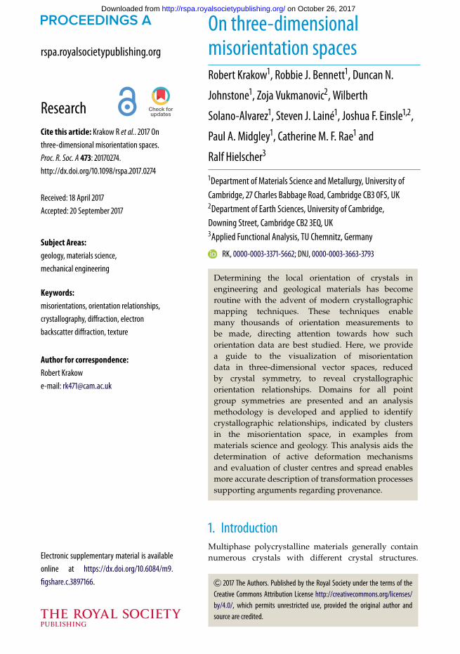
Rotations may also be represented by the axis and angle of rotation. (Mis)orientationdistributions can be expanded in these terms [58,59] and the representation is intuitive. A series ofso-called neo-Eulerian mappings have been defined, based on this notion, as 3D vectors formedby scaling a unit vector, ξ , parallel to the axis of rotation by a function of the rotation angle, ω,about that axis, f (ω). The choice of the scaling function, f (ω), conveys particular properties onthe resulting vector space. Five suggestions were made by Frank [44,60], as follows:

Axis-angle, v = ωξ : Simple and the angular units ease direct interpretation.5

Rodrigues–Frank, r = tan(ω/2)ξ : Rectilinear, i.e. rotation about a given axis is a straightline through any point. Some domains are unbounded since the scaling function tends toinfinity.Conformal, c = 2 tan(ω/4)ξ : Equal angle projection of S

3 onto Euclidean space. Theconfiguration in any small region of the map is geometrically similar to that which itwould have, if transferred to any other point in the map.Homochoric, z = { 3

4 (ω − sin ω)}1/3ξ : Equivalent of the equal area plane map of a sphereand can be considered an equal volume projection of S

3 onto Euclidean space. Thedeterminant of the metric tensor is preserved and a random distribution of orientations

5It is noteworthy that some authors have applied a factor of 2 scaling to the rotational angle in the axis-angle representationin order to make the Taylor expansion of all neo-Eulerian mappings more similar at low angles. We have not adopted thisconvention here as we find the vector magnitude being directly the rotational angle to be convenient in a pragmatic sense.



5


...................................................

will have equal probabilities of being found within equal volume elements anywhere inthe map [44].6

Quaternion vector, q = sin(ω/2)ξ : Enclosed within a sphere of unit radius and easily relatedto the quaternion representation, described above, for computations.

The neo-Eulerian mappings each offer certain advantages. In particular, the rectilinearity ofthe Rodrigues–Frank representation has made it popular although the unbounded nature offundamental zones containing rotations of 180◦ is a practical issue for low symmetry systems.The homochoric representation is attractive for visualization owing to the equal distribution ofrandomly distributed points [17]. Analysis principles developed in this work apply equally wellto all neo-Eulerian mappings, which have all been made available in the open-source MTEXtoolbox so that readers may make the most appropriate choice for their needs. Here, we apply theaxis-angle parametrization because it is sufficient to illustrate the important principles, boundedin low-symmetry cases, and the magnitude of the vector is directly the misorientation angle whichsimplifies at-a-glance interpretation.

3. Fundamental zones and crystal symmetryCrystal symmetry implies that some (mis)orientations are physically indistinguishable. However,equivalent (mis)orientations will be represented by different points in the 3D vector space whenexpressed as neo-Eulerian vectors. It is only necessary to use a region of the vector spacecontaining each physically distinct (mis)orientation precisely once. Such a region is known asa fundamental zone [4,33,44] or an asymmetric domain [16]. In this section, a consistent definition forthe fundamental zone is set out and fundamental zones are tabulated for all crystal symmetries.

Fundamental zones have previously been specified by a number of authors based onRodrigues–Frank parameters [4,16,33]. Here, the calculation was instead achieved following aconstruction based on quaternion geometry, as detailed in appendix A. The fundamental zonemay then be transformed into any of the neo-Eulerian representations. These representationsdiffer geometrically, as discussed in §2. The scaling functions, f (ω), shown in figure 2a, are allapproximately linear up to approximately 1 radian and then diverge. The bounding surfaces ofthe fundamental zone are curved in all cases except Rodrigues–Frank, see figure 2b, reflecting theaforementioned rectilinearity.

The particular fundamental zone obtained depends on the alignment of axes and the order inwhich symmetry operators are combined for misorientations. The standard settings, consistentwith the International Tables for Crystallography, are followed here and these conventionsare detailed in appendix B. The importance of these alignments cannot be understated sinceinconsistent adoption of conventions for these alignments can cause much confusion in applyingthe methods described here.

(a) Symmetry equivalence of (mis)orientationsCalculation of the fundamental zone is based on selecting, from symmetry equivalent points, thepoint closest to the origin (smallest angle of rotation) and rejecting more remote points. Whenmultiple equivalent points have the same distance to the origin, a constraint is placed on thedirection of the axis of rotation. To express this mathematically, it is noted that crystal coordinatesare subject to symmetry described by the group of symmetry operators, s, comprising thecrystallographic point group S. A symmetry operation applied to the crystal coordinates producesa physically identical configuration and therefore the crystal coordinates h can be identified witha set sh (s ∈ S) of symmetrically equivalent crystal coordinates.7 Considering equation (2.1) yields

6The homochoric mapping is also related to the so-called cubochoric mapping in which efficient division of the space ispossible [61].7Some authors [53] have suggested applying symmetry to the specimen coordinate system, but this can be confusing withrespect to misorientations and is avoided in this work.



6


...................................................

0

1.5

1 2 30

1

2

3

angle of rotation w (rad)

f(w

)axis-angle

Rodrigues–Frank

conformal

homochoric

quaternion

e1

w (r

ad)

w (rad) w (rad)1.5

–1.5

1.5

0

e3

e2

(b)(a)

–1.50

Figure 2. (a) The scaling function for five neo-Eulerian orientation mappings as a function of the rotational angle. Themaximum angle for 222 symmetry is 2π /3 radians (120◦) in [111] direction (indicated by red dotted lines). (b) Sectionedfundamental zone for 222 symmetry in each of the five neo-Eulerian mappings, illustrating differences in geometry.

the following expression for symmetrically equivalent orientations,

g = gs, s ∈ S. (3.1)

Misorientations are subject to the symmetry operations of crystallographic point groups, S1and S2, associated with the crystal coordinate systems, h1 and h2, which are related by themisorientation, m. Considering the effect of symmetry on each crystal coordinate system, asdescribed above, and using equation (2.3), the following expression for symmetrically equivalentmisorientations is obtained.

m = s2ms1, s1 ∈ S1, s2 ∈ S2. (3.2)

Unique selection of a misorientation (referred to as the disorientation) to represent allsymmetrically equivalent misorientations8 requires a constraint on both the angle of rotationand axis of rotation because several symmetrically equivalent misorientations may have thesame rotational angle.9 Here, the misorientation with the smallest angle of rotation (knownas the disorientation angle) and an axis of rotation within the inverse pole figure (IPF) sectorcorresponding to the point group of common symmetries, SC = S1 ∩ S2, is chosen.

(b) Relating symmetry to fundamental zonesConstruction of the fundamental zone may be understood by considering that the symmetryoperators map the reference (mis)orientation or identity, which is at the origin of the 3D vectorspace, to a set of identity equivalent points throughout the vector space following equations(3.1) and (3.2). The fundamental zone then comprises the set of points that are closer to theidentity at the origin than any of the other identity equivalent points. Indeed, this is preciselythe notion used by Morawiec [16] and in this work (appendix A) to compute the fundamentalzone. This view of the construction is similar to that commonly used to describe the BrillouinZone in reciprocal space and helps to rationalize the observed shapes of the fundamental zone,as below.

Fundamental zones for orientations involve only one set of symmetry operators accordingto equation (3.1). This is also equivalent to the formation of a misorientation fundamental zone

8If the crystallographic point groups S1, S2 comprise N1 and N2 symmetry elements, then each misorientation generally hasN1 × N2 symmetry equivalents.9Specifically, if we denote SC = S1 ∩ S2 the group of common symmetries of S1 and S2. Then for any misorientation m withrotational angle ω(m) and rotational axis ξ (m), the symmetrically equivalent misorientations s m s−1, s ∈ Sc have the samerotational angle ω(sms−1) = ω(m) but different rotational axis ξ (sms−1) = sξ (m).



7


...................................................

e3||c*

e3||c*

e1||a

e1||a

e2||b

c

ba

0

e3

e3w

(°)

w (°)w (°)

w (°)w (°)

w (°

)c

b

a

0b

222

622

e2e1

e2

e2

e1

150

100

50

0

–50

–100

–100100

1000

–100

1000

–100

0

–1001000

–150

150

100

50

0

–50

–100

–150

(b)

(a)

(c)(d )

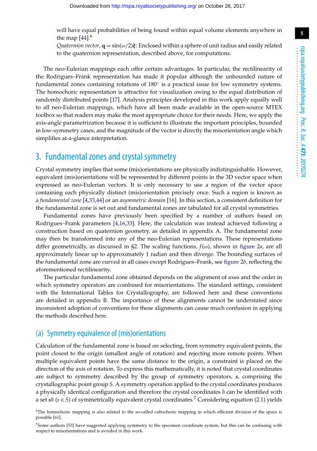
Figure 3. (a,c) Stereographic projections of symmetry elements and corresponding symmetry reduced fundamental zones (b,d)in axis-angle space for: (a,b) orientations of crystals with point group 222 (c,d) orientations of crystals with point group 622.

when S2 = 1. A two-fold symmetry axis produces an identity equivalent point at a position180◦ from the origin along the symmetry axis. Points up to 90◦ from the origin along thisaxis are clearly closer to the identity at the origin than to the identity equivalent point andtherefore the boundary of the fundamental zone is at 90◦ along this axis. This idea extendseasily to other rotational symmetry operators with triads, tetrads and hexads each producingidentity equivalent points at 120◦, 90◦ and 60◦ along the respective symmetry axis. Visualizingthe curvature of the bounding surfaces of the fundamental zone is more difficult and dependson the particular representation chosen. The principle is to construct the surface correspondingto rotation about axes orthogonal to the symmetry axis and passing through the easily definedbounding point on the symmetry axis. The inner envelope of these surfaces will then define thefundamental zone.

Considering the 222 point group, the diad operators constrain the domain to ±90◦ alongthe coordinate axes producing a convex cube, as shown in figure 3b. For the 622 pointgroup, the hexad operator constrains the domain to ±30◦ along e3 and the diad operatorsconstrain the domain to ±90◦ along each of the corresponding axes, as shown in figure 3d. Itis, therefore, reasonably intuitive to deduce the qualitative shape of the fundamental zone fororientations.

Fundamental zones for misorientations when both crystals contribute symmetry operators areformed in two different ways depending on whether the symmetry groups contain common



8


...................................................

w (°)

w (°)

w (°)

40

40 50

0

–50

30

1st: 4322nd: 3

1st: 6222nd: 222

20

20

20

100

0

0

–10–20

–20

–20

–30–40

–40

–50500

w (°

)w

(°)

e3

e3

e2e1

w (°)500

–50

e1e2

(b)(a)

(c)

(d )

Figure 4. Stereographic projections (a,c) of symmetry elements and corresponding symmetry reduced fundamental zonesof axis-angle space (b,d) for: (a,b) misorientations of crystals with point group (PG) 432 and combination of PGs 432-3 (c,d)misorientations of crystals with PG 622 and combination of 622-222.

elements as discussed in more detail by Morawiec [16]. When the two symmetry groups donot contain any common elements, then there are no symmetry equivalent misorientations withthe same misorientation angle and the fundamental zone is again constructed by selectingthe misorientation closest to the origin. This is the case for the 432-3 fundamental zoneshown in figure 4a,b. If the symmetry groups do contain common elements, then there will besymmetry equivalent misorientations with the same angle of rotation and the restriction on themisorientation axis discussed above is required. This is the case for the 622-222 fundamentalzone shown in figure 4c,d. All of the symmetrically equivalent misorientations with the samemisorientation angle lie within the higher symmetry 622 fundamental zone. Each diad from the222 point group then effectively excludes half of the space. However, a pair of diads implies thethird and therefore the fundamental zone is 1

4 the original domain rather than 18 . The particular

segments defining the fundamental zone correspond to the defined IPF segment.The segmentation seen in figure 4d leads to a notion of domain geometries where the

fundamental zone is either (i) one of the domain geometries (e.g. figure 3 or 4b) or (ii) a segmentof it, produced by cutting with planes often parallel to e1, e2 or e3, as in figure 4d. This makes ittractable to discuss fundamental zones for all crystal combinations, as follows.

(c) Fundamental zones for all crystalsCrystals possess point group symmetry described by one of the 32 crystallographic point groups.Eleven of these point groups are proper point groups and only contain symmetry operations that



9


...................................................

Table 1. Fundamental zones for misorientations expressed as sections of the domain geometries shown in figure 5 for allcombinations of proper point group symmetry operators, which are listed in Hermann–Mauguin notation [6]. The self-symmetry combinations (highlighted) donot include so-called grain exchange symmetry,whichwould halve the domain space.

432 23 622 6 32 3 422 4 222 2 1

1 c d f k h m g l i n o. . . . . . . . . . . . . . . . . . . . . . . . . . . . . . . . . . . . . . . . . . . . . . . . . . . . . . . . . . . . . . . . . . . . . . . . . . . . . . . . . . . . . . . . . . . . . . . . . . . . . . . . . . . . . . . . . . . . . . . . . . . . . . . . . . . . . . . . . . . . . . . . . . . . . . . . . . . . . . . . . . . . . . . . . . . . . . . . . . . . . . . . . . . . . . . . . . . . . . . . . .

2 c/2 d/2 f /2 f f h g/2 g i/2 n/2. . . . . . . . . . . . . . . . . . . . . . . . . . . . . . . . . . . . . . . . . . . . . . . . . . . . . . . . . . . . . . . . . . . . . . . . . . . . . . . . . . . . . . . . . . . . . . . . . . . . . . . . . . . . . . . . . . . . . . . . . . . . . . . . . . . . . . . . . . . . . . . . . . . . . . . . . . . . . . . . . . . . . . . . . . . . . . . . . . . . . . . . . . . . . . . . . . . . . . . . . .

222 c/4 d/4 f /4 f /2 f /2 f g/4 g/2 i/4. . . . . . . . . . . . . . . . . . . . . . . . . . . . . . . . . . . . . . . . . . . . . . . . . . . . . . . . . . . . . . . . . . . . . . . . . . . . . . . . . . . . . . . . . . . . . . . . . . . . . . . . . . . . . . . . . . . . . . . . . . . . . . . . . . . . . . . . . . . . . . . . . . . . . . . . . . . . . . . . . . . . . . . . . . . . . . . . . . . . . . . . . . . . . . . . . . . . . . . . . .

4 c/4 c/2 e/2 j/2 e j g/4 l/4. . . . . . . . . . . . . . . . . . . . . . . . . . . . . . . . . . . . . . . . . . . . . . . . . . . . . . . . . . . . . . . . . . . . . . . . . . . . . . . . . . . . . . . . . . . . . . . . . . . . . . . . . . . . . . . . . . . . . . . . . . . . . . . . . . . . . . . . . . . . . . . . . . . . . . . . . . . . . . . . . . . . . . . . . . . . . . . . . . . . . . . . . . . . . . . . . . . . . . . . . .

422 c/8 c/4 e/4 e/2 e/2 e g/8. . . . . . . . . . . . . . . . . . . . . . . . . . . . . . . . . . . . . . . . . . . . . . . . . . . . . . . . . . . . . . . . . . . . . . . . . . . . . . . . . . . . . . . . . . . . . . . . . . . . . . . . . . . . . . . . . . . . . . . . . . . . . . . . . . . . . . . . . . . . . . . . . . . . . . . . . . . . . . . . . . . . . . . . . . . . . . . . . . . . . . . . . . . . . . . . . . . . . . . . . .

3 a b f /3 k/3 h/3 m/3. . . . . . . . . . . . . . . . . . . . . . . . . . . . . . . . . . . . . . . . . . . . . . . . . . . . . . . . . . . . . . . . . . . . . . . . . . . . . . . . . . . . . . . . . . . . . . . . . . . . . . . . . . . . . . . . . . . . . . . . . . . . . . . . . . . . . . . . . . . . . . . . . . . . . . . . . . . . . . . . . . . . . . . . . . . . . . . . . . . . . . . . . . . . . . . . . . . . . . . . . .

32 a/2 b/2 f /6 f /3 h/6. . . . . . . . . . . . . . . . . . . . . . . . . . . . . . . . . . . . . . . . . . . . . . . . . . . . . . . . . . . . . . . . . . . . . . . . . . . . . . . . . . . . . . . . . . . . . . . . . . . . . . . . . . . . . . . . . . . . . . . . . . . . . . . . . . . . . . . . . . . . . . . . . . . . . . . . . . . . . . . . . . . . . . . . . . . . . . . . . . . . . . . . . . . . . . . . . . . . . . . . . .

6 a/2 b/2 f /6 k/6. . . . . . . . . . . . . . . . . . . . . . . . . . . . . . . . . . . . . . . . . . . . . . . . . . . . . . . . . . . . . . . . . . . . . . . . . . . . . . . . . . . . . . . . . . . . . . . . . . . . . . . . . . . . . . . . . . . . . . . . . . . . . . . . . . . . . . . . . . . . . . . . . . . . . . . . . . . . . . . . . . . . . . . . . . . . . . . . . . . . . . . . . . . . . . . . . . . . . . . . . .

622 a/4 b/4 f /12. . . . . . . . . . . . . . . . . . . . . . . . . . . . . . . . . . . . . . . . . . . . . . . . . . . . . . . . . . . . . . . . . . . . . . . . . . . . . . . . . . . . . . . . . . . . . . . . . . . . . . . . . . . . . . . . . . . . . . . . . . . . . . . . . . . . . . . . . . . . . . . . . . . . . . . . . . . . . . . . . . . . . . . . . . . . . . . . . . . . . . . . . . . . . . . . . . . . . . . . . .

23 c/12 d/12. . . . . . . . . . . . . . . . . . . . . . . . . . . . . . . . . . . . . . . . . . . . . . . . . . . . . . . . . . . . . . . . . . . . . . . . . . . . . . . . . . . . . . . . . . . . . . . . . . . . . . . . . . . . . . . . . . . . . . . . . . . . . . . . . . . . . . . . . . . . . . . . . . . . . . . . . . . . . . . . . . . . . . . . . . . . . . . . . . . . . . . . . . . . . . . . . . . . . . . . . .

432 c/24. . . . . . . . . . . . . . . . . . . . . . . . . . . . . . . . . . . . . . . . . . . . . . . . . . . . . . . . . . . . . . . . . . . . . . . . . . . . . . . . . . . . . . . . . . . . . . . . . . . . . . . . . . . . . . . . . . . . . . . . . . . . . . . . . . . . . . . . . . . . . . . . . . . . . . . . . . . . . . . . . . . . . . . . . . . . . . . . . . . . . . . . . . . . . . . . . . . . . . . . . .

are proper rotations. The remaining crystallographic point groups contain improper symmetryoperations that involve inversion. Treatment of improper operations has varied somewhatbetween authors. Here, we adopt the convention in which the crystals may only be related bya proper rotation operation and therefore only the proper point groups must be considered. Acorrespondence table between the Laue class of a crystal and the appropriate proper point groupfor definition of the fundamental zone is provided in appendix C to inform the correct choice.

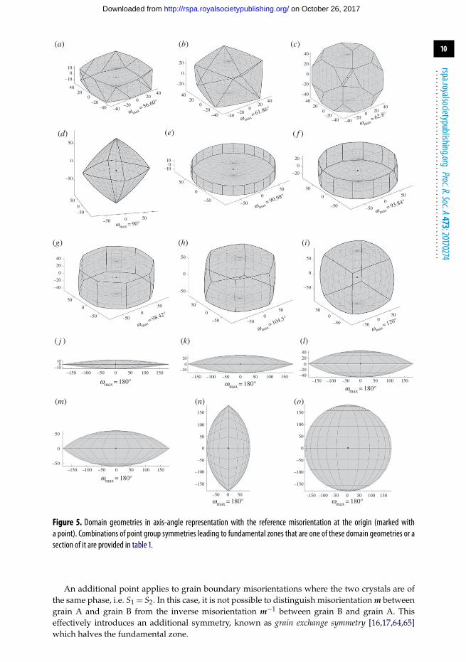
Fundamental zones for all proper point group combinations were computed and it was foundthat 15 distinct domain geometries occur, as shown in figure 5a–o, for increasing maximum angle ofrotation. The correspondence between fundamental zones for misorientations and these domaingeometries is summarized in table 1.

Of the 15 domain geometries, 11 (all excluding figure 5a,b,e,j) correspond directly to thefundamental zones for orientations and, equivalently, misorientations with S2 = 1. The effectof rotational symmetry operators in truncating the orientation space perpendicular to theaxis of rotation can be identified in each case, as discussed in the previous section. This isparticularly clear for the lenticular fundamental zones (figure 5o,n,m,l,k) which are formed withthe application of: no symmetry, a diad axis, a triad axis, a tetrad axis, and a hexad axis parallel tothe short axis of the fundamental zone. The maximum misorientation angle (from the centre)along the axis parallel to this symmetry axis is then limited to 180◦, 90◦, 60◦, 45◦ and 30◦,respectively. Conventional crystallographic settings, with the monoclinic diad parallel to e2 resultin domain n being truncated along the e2 axis, whereas others are truncated along e3.

Fundamental zones for misorientations combining proper point groups that do not possesscommon symmetry elements define new domain geometries centred around the origin, asdescribed above. These are the domain geometries in figure 5a,b,e,j. In all other cases, thefundamental zone is a segment of one of these 15 domain geometries with a volume indicated bythe associated fraction in table 1. The fundamental zones calculated in this work agree with thosereported for various proper point group combinations [4,16,17,30,62,63] when differences in axisalignment are accounted for. Here, conventions for axis alignment and the order of symmetryoperations have been clearly set out (§3 and appendix B) and the fundamental zone has beenreduced to the minimal disorientation space in all cases. The explicit statement of consistent‘standard’ conventions is practically significant when comparing multiple datasets.



10


...................................................

(i)

w max= 120°

5050

50

0

0

–50–50

–50

0

(h)

w max= 104.5°

5050

0

–50–50

–50

50

0

0

(d)

wmax = 90°

50

50

50

–50

–50

–50

0

0

0

(m)

wmax = 180°

–50

50

0

–150 –100 –50 0 50 100 150

(n)

wmax = 180°

150

–150

0

50

–50

100

–100

–50 0 50

(o)

wmax = 180°–150

–150

–100

–50

0

50

–100 –50 0 50 100

100

150

150

( j )

wmax = 180°

–10–150 –100 –50 0 50 100 150

100

(k)

wmax = 180°–150 –100 –50 0 50 100 150

–20

20

0

(l)

wmax = 180°–150 –100 –50 0 50 100 150

–40–20

02040

(e)

w max= 90.98°

100

–10

50

–50

0 50

–50

0

( f )

20

0

–20

w max= 93.84°

50

50

–50 –50

00

(g)

w max= 98.42°

–40

40

20

0

–20

5050

0

–50–500

(a)

100

–10

4040

w max= 56.60°

20200

0–20–20–40 –40

(b)

20

0

–20

w max= 61.86°

4020

0–20

–40

4020

0–20

–40

(c)

w max= 62.8°

4020

0–20

–40

40

20

0

–20

–40

4020

0–20

–40

Figure 5. Domain geometries in axis-angle representation with the reference misorientation at the origin (marked witha point). Combinations of point group symmetries leading to fundamental zones that are one of these domain geometries or asection of it are provided in table 1.

An additional point applies to grain boundary misorientations where the two crystals are ofthe same phase, i.e. S1 = S2. In this case, it is not possible to distinguish misorientation m betweengrain A and grain B from the inverse misorientation m−1 between grain B and grain A. Thiseffectively introduces an additional symmetry, known as grain exchange symmetry [16,17,64,65]which halves the fundamental zone.



11


...................................................

30°

1 2

3

4 1

2

3

90°

(b)(a)

(c) (d )

Figure 6. Properties ofmisorientation clusters situated at the bounding surface of the cubic (m3̄m) to trigonal (3̄) fundamentalzone (domain a). This is illustrated by colouring similarmisorientationswith equal colours for each image separately. (a) Clustersreappearing at an opposite boundary face, either directly opposite or opposite and rotated; (b) clusters at a corner reappearingat another corner; (c) clusters that do not reappear in a different position; (d) clusters at edges and triple points can split intomore than two clusters.

(d) Boundaries of the fundamental zoneThe fundamental zone contains each symmetrically equivalent misorientation once. In the interiorof the fundamental zone, the vector space behaves approximately like the ordinary 3D Euclideanspace. In particular, misorientations clustering randomly around a fixed orientation relationshipappear as one cloud. However, when plotting the fundamental zone as a bounded domain in3D space, it is important to consider a misorientation lying on the boundary and the appearancewhen a cluster of misorientations crosses the boundary.

A misorientation lying on the boundary of the fundamental zone is equivalent to anothermisorientation on the boundary with the same rotational angle [44]. A cluster crossing theboundary will, therefore, reappear at this symmetry equivalent boundary point. This is similar, inprinciple, to crossing the boundary of a Brillouin zone in reciprocal space. However, the topologyof the space is more complicated for orientations and rotations are also involved. The mostcommon situation is that a cluster reappears just at the opposite face, but rotated about the facecentre, as shown in figure 6a for the 432-3 fundamental zone. A cluster crossing the fundamentalzone boundary at a corner typically reappears at a different corner, as shown in figure 6b. Atsome edges (and corners in other fundamental zones), the cluster may re-enter at an immediatelyadjacent point, as shown in figure 6c. Finally, less intuitive splitting can occur including: re-entrythrough a nearby face and splitting into more than two clusters, as shown in figure 6d.

In cases where clusters cross the fundamental zone boundary, visualization may be aidedsignificantly by colouring symmetry-related clusters based on misorientation from a suspectedorientation relationship or a cluster centre, as shown in figure 6. It can also be helpful to inspectthe symmetrized dataset prior to reducing the data to the fundamental zone as it is the application



12


...................................................

e3

e2e1

1st: 4322nd: 3

triadsparallel

cubic tetrad parallel totrigonal triad

w (°

)

40

4060

20

20

0

0

–20

–20

–40

–40

–60

–6050

0–50

w (°)w (°)

(b)(a)

(c)(d )

Figure 7. (a) Stereographic projection of symmetry elements for cubic (m3̄m) and trigonal (3̄) point groups with triad axesparallel to e3. (b) Corresponding symmetry reduced fundamental zones (c), clusters at vertices, (d) clusters along the triad axis(e3-axis). Set-up highlights that the four misorientations are rotations about e3-axis (c.f. §4).

of symmetry that results in the splitting. Finally, it may be advantageous to move away from‘standard’ conventions for the fundamental zone definition to better reflect the data, as follows.

(e) Alternative axis alignmentsAdopting ‘standard’ conventions for the alignment of coordinate and symmetry axes hasthe advantage of familiarity with a misorientation space and enables direct comparisonbetween datasets. However, alternative axis alignments may simplify the interpretation ofdata by reflecting underlying crystallographic symmetry [16]. For example, the cubic–trigonalfundamental zone for misorientations has the trigonal triad axis and the cubic tetrad axis alignedfollowing the standard conventions, as shown in figure 4a,b. Crystallographically, it may makesense to align the triad axes of the trigonal and cubic systems, as illustrated in figure 7a,b.This alternative alignment leads to a fundamental zone of geometry c/3, whereas the standardalignment leads to geometry a. The alignment of triad axes is particularly advantageous ifthese symmetry axes are aligned in important crystallographic orientation relationships. In thisalternative alignment, misorientations about the triad axis are situated along the e3 axis ratherthan at vertices in the standard fundamental zone, as shown in figure 7c,d.

4. Orientation relationships revealed in misorientation spaceCrystallographic orientation relationships, arising throughout materials and earth sciences, maybe visualized in 3D misorientation spaces. Here, the utility of this approach is illustrated



13


...................................................

10 mm (011)

(001)

(111)

(a) (b)

Figure 8. Nanostructured bainite [69], IPF colour code with regard to z-axis for both maps in the inlay. (a) Orientation map offerrite laths in IPF colours. Several orientations of laths occur within a prior austenite grain. (b) Orientation map of the retainedaustenite phase in IPF colours.

using examples selected to incorporate important materials systems and a range of crystalsymmetries. For each example, a minimal introduction to the key microstructural features isprovided and the data, as well as extended analysis scripts, have been made available [48].The orientation mapping data were obtained via electron backscatter diffraction (EBSD) usingconventional Hough-transform-based analysis, which conveys a (mis)orientation measurementprecision on the order of approximately 1◦ [66]. Orientation relationships are assessed bycalculating misorientations between all combinations of phases present and plotting them inthe respective fundamental zone. When particular crystallographic orientation relationships arepreferred, numerous disorientations will be observed to occur close to a particular point inthe fundamental zone. The mean of such a cluster of disorientations can then be determinedand this is achieved here using the iterative procedure described by Bachmann et al. [67].Typically, such disorientation clusters contain greater than 100 discrete measurements and themean can, therefore, be determined with a precision of approximately 0.1◦. Often cluster centerswill be close to a disorientation corresponding to the parallelism of low Miller index planesand directions, which relates the analysis back to more traditional approaches and makes iteasier to visualize approximate atomic structures. Finally, boundary segments associated withdisorientations in selected clusters may be plotted to assess the microstructural distribution ofparticular disorientations.

(a) Orientation relationships in nanostructured bainitic steelNanostructured bainitic steels typically contain key alloying additions of Si, Mn and Ni andthe mechanical properties obtained offer a balance of strength and toughness attractive in manyapplications. The sample studied here was developed for rolling contact fatigue properties [68] asa bearing steel and is described further by Solano et al. [69]. The microstructure comprises a densedistribution of ferrite, α-Fe, (m3̄m, space group 229) laths in prior austenite, γ -Fe, (m3̄m, spacegroup 225) grains, as shown in figure 8. Iron carbides were not observed [69]. Ferrite laths accountfor approximately 84% of indexed pixels, whereas retained austenite makes up approximately16%. This is sufficient to recognize the prior austenite grains in figure 8b. At least three variants(colours) of ferrite laths are present in each austenite grain, indicating different transformationdirections although the full number is not evident from a single IPF coloured map.

Multiple ferrite orientations occur within each prior austenite grain because the transformationfrom austenite to ferrite can start at any of the equivalent {111}γ planes and occur in any of three



14


...................................................

P

NW

KS

(100)

CSL3

CSL9

CSL11

CSL7

(110)

projection||(001) projection||(001)

(010)

(010)

NW-NWKS-KSKS-NW

w (°

)

w (°) w (°)

sc1

sc2

sc3

sc4

40

35

30

25

20

15

10

5

0–30 –20–40 –10 0 0–5–10–15–20–25–30

40

35

30

25

20

15

10

5

0

–

(b)(a)

Figure 9. Misorientation distributions of nanostructured bainite in axis-angle space (a) Austenite–ferrite distribution withcluster situated between NW and KS (b) Ferrite–ferrite distribution with cluster above CSL11. Orientation relationships and CSLsare annotated (table 2).

Table 2. List of common orientation relationships, ferrite–ferrite boundary misorientations and CSL boundaries (forcombinations of fcc-fcc and bcc-bcc) used in the analysis [28,71–73].

orientation relationship definition of misorientation

Kurdjumov–Sachs (KS) (111)γ ‖(011)α , [1̄01]γ ‖[1̄1̄1]α. . . . . . . . . . . . . . . . . . . . . . . . . . . . . . . . . . . . . . . . . . . . . . . . . . . . . . . . . . . . . . . . . . . . . . . . . . . . . . . . . . . . . . . . . . . . . . . . . . . . . . . . . . . . . . . . . . . . . . . . . . . . . . . . . . . . . . . . . . . . . . . . . . . . . . . . . . . . . . . . . . . . . . . . . . . . . . . . . . . . . . . . . . . . . . . . . . . . . . . . . .

Nishiyama–Wassermann (NW) (111)γ ‖(011)α , [112̄]γ ‖[01̄1]α. . . . . . . . . . . . . . . . . . . . . . . . . . . . . . . . . . . . . . . . . . . . . . . . . . . . . . . . . . . . . . . . . . . . . . . . . . . . . . . . . . . . . . . . . . . . . . . . . . . . . . . . . . . . . . . . . . . . . . . . . . . . . . . . . . . . . . . . . . . . . . . . . . . . . . . . . . . . . . . . . . . . . . . . . . . . . . . . . . . . . . . . . . . . . . . . . . . . . . . . . .

Pitsch (P) (010)γ ‖(101)α , [101]γ ‖[1̄11]α. . . . . . . . . . . . . . . . . . . . . . . . . . . . . . . . . . . . . . . . . . . . . . . . . . . . . . . . . . . . . . . . . . . . . . . . . . . . . . . . . . . . . . . . . . . . . . . . . . . . . . . . . . . . . . . . . . . . . . . . . . . . . . . . . . . . . . . . . . . . . . . . . . . . . . . . . . . . . . . . . . . . . . . . . . . . . . . . . . . . . . . . . . . . . . . . . . . . . . . . . .

cluster centre 44.2◦about [−0.1917, 0.0996, 0.9764]γ. . . . . . . . . . . . . . . . . . . . . . . . . . . . . . . . . . . . . . . . . . . . . . . . . . . . . . . . . . . . . . . . . . . . . . . . . . . . . . . . . . . . . . . . . . . . . . . . . . . . . . . . . . . . . . . . . . . . . . . . . . . . . . . . . . . . . . . . . . . . . . . . . . . . . . . . . . . . . . . . . . . . . . . . . . . . . . . . . . . . . . . . . . . . . . . . . . . . . . . . . .

NW–NW boundary, same {111}γ 60◦about [011]. . . . . . . . . . . . . . . . . . . . . . . . . . . . . . . . . . . . . . . . . . . . . . . . . . . . . . . . . . . . . . . . . . . . . . . . . . . . . . . . . . . . . . . . . . . . . . . . . . . . . . . . . . . . . . . . . . . . . . . . . . . . . . . . . . . . . . . . . . . . . . . . . . . . . . . . . . . . . . . . . . . . . . . . . . . . . . . . . . . . . . . . . . . . . . . . . . . . . . . . . .

KS–NW boundary, same {111}γ 54.7◦about [011]. . . . . . . . . . . . . . . . . . . . . . . . . . . . . . . . . . . . . . . . . . . . . . . . . . . . . . . . . . . . . . . . . . . . . . . . . . . . . . . . . . . . . . . . . . . . . . . . . . . . . . . . . . . . . . . . . . . . . . . . . . . . . . . . . . . . . . . . . . . . . . . . . . . . . . . . . . . . . . . . . . . . . . . . . . . . . . . . . . . . . . . . . . . . . . . . . . . . . . . . . .

CSL3 and CSL7* 60◦ and 38.2◦about [111]. . . . . . . . . . . . . . . . . . . . . . . . . . . . . . . . . . . . . . . . . . . . . . . . . . . . . . . . . . . . . . . . . . . . . . . . . . . . . . . . . . . . . . . . . . . . . . . . . . . . . . . . . . . . . . . . . . . . . . . . . . . . . . . . . . . . . . . . . . . . . . . . . . . . . . . . . . . . . . . . . . . . . . . . . . . . . . . . . . . . . . . . . . . . . . . . . . . . . . . . . .

CSL5* 36.9◦about [001]. . . . . . . . . . . . . . . . . . . . . . . . . . . . . . . . . . . . . . . . . . . . . . . . . . . . . . . . . . . . . . . . . . . . . . . . . . . . . . . . . . . . . . . . . . . . . . . . . . . . . . . . . . . . . . . . . . . . . . . . . . . . . . . . . . . . . . . . . . . . . . . . . . . . . . . . . . . . . . . . . . . . . . . . . . . . . . . . . . . . . . . . . . . . . . . . . . . . . . . . . .

CSL9 and CSL11* 38.9◦ and 50.5◦about [011]. . . . . . . . . . . . . . . . . . . . . . . . . . . . . . . . . . . . . . . . . . . . . . . . . . . . . . . . . . . . . . . . . . . . . . . . . . . . . . . . . . . . . . . . . . . . . . . . . . . . . . . . . . . . . . . . . . . . . . . . . . . . . . . . . . . . . . . . . . . . . . . . . . . . . . . . . . . . . . . . . . . . . . . . . . . . . . . . . . . . . . . . . . . . . . . . . . . . . . . . . .

〈110〉γ directions in each of those planes. Typically, the most densely packed atomic planes in eachphase ({110}α and {111}γ ) remain nearly parallel [70]. However, the existence of an invariant line,necessary for a glissile interface, requires a shear transformation and a rigid body rotation. Theinvariant line requirement implies that the habit plane and the resulting orientation relationshipmust have irrational Miller indices. Several orientation relationships are listed in table 2, but areonly approximate. Therefore using 3D misorientation space, the distinction between experimentaldata and these approximations becomes clear.

Austenite-ferrite misorientations in this sample are clustered between the Nishiyama–Wassermann (NW) and Kurdjumov–Sachs (KS) orientation relationships, as shown in figure 9a.The radius of the cluster is 2.7◦, indicating a misorientation spread greater than the precisionof the experiment. This is consistent with other studies on carbide-free bainite [28]. For upperbainite, distributions between KS and NW have been observed, while for lower bainite, a widermisorientation distribution has been observed [74]. The centre of this austenite-ferrite clusterwas determined to be 44.2◦ approximately [−0.1917, 0.0996, 0.9764], which is 1.9◦ away from the



15


...................................................

NW orientation relationship that is the closest low-index parallelism. However, the cluster centreprovides a more accurate description of the transformation process than any of the establishedORs, which is evidenced by the fact that 62.0% of all misorientations are situated at a 2◦ distancefrom that centre compared to 28.2% and 2.6% for NW and KS, respectively.10 Smaller clusters(sc1–sc4) were found to belong to isolated pixels not clearly associated with the transformation.

Ferrite–ferrite misorientations are cluster centred around a misorientation of 56◦ about the[011] axis (red arrow). This cluster appears primarily to be a direct consequence of the austenite toferrite transformation process, described above. This leads to particular misorientations betweenferrite laths within any given prior austenite grain and it is clear by the inspection of theorientation maps that the majority of ferrite–ferrite boundaries are situated within prior austenitegrains and so dominate the statistics. Flower et al. [73] calculated the expected ferrite–ferritemisorientations between two NW-type laths formed in the same parent austenite grain to be 60◦about [011] (same for two KS laths) and 54.7◦ about [011] for a KS lath in contact with a NWvariant. These are indicated by blue and green arrows, in figure 9b. Like the austenite–ferritemisorientations then the observed ferrite–ferrite misorientation cluster at 56◦ about the [011] axisis therefore most accurately described with a single cluster of austenite–ferrite misorientationsbetween KS and NW. It is neither a consequence of identical boundary types (60◦) nor stronglydissimilar boundaries (54.7◦) only. Further, it is noteworthy that he clustering of ferrite–ferritemisorientations may provide a clear criterion for the reconstruction of prior austenite grains.

This case study demonstrates the utility of 3D misorientation spaces in providing a descriptionof the austenite–ferrite transformation that is more consistent with the physical nature of thetransformation, which would lead to representation in terms of irrational Miller indices. Thedescription of the orientation relationship as being around the cluster centre is also more accuratein the sense that 61.9% of all misorientations are situated within a distance of 2◦ of the determinedcentre, whereas only 28.2% are situated around NW and 2.6% are situated around KS. Finally, thisexample illustrates the application of grain exchange symmetry for misorientations between thesame phase crystals, which halves the domain space for ferrite–ferrite misorientations comparedto austenite–ferrite misorientations (see appendix B).

(b) Deformation twinning in titanium during high strain ratesDeformation twinning occurs in hexagonal close packed (h.c.p.) titanium (6/mmm, space group194) as is typical in h.c.p. metals in order to satisfy the criterion of five independent slip systemsfor general plastic deformation [75]. Four independent systems are provided by 〈a〉 type slipwithin basal {0001}, prismatic {11̄00} or pyramidal {11̄01} planes. Slip activation and hencestrain accommodation parallel to the c-axis, however, must occur via 〈c + a〉 type slip along thepyramidal planes, {11̄01} and {112̄2}, in the 〈112̄3〉 directions. The critically resolved shear stressfor 〈c + a〉 slip to occur is known to be far greater than for the four other slip systems [76] andtherefore deformation parallel to the c-axis is largely accommodated by deformation twinning.The deformation twinning modes considered active in h.c.p. titanium are listed in table 3.

According to the calculations by Bonnet et al. [20], there are near CSL misorientations whichhave been used to describe twinning misorientations in Ti [78]. It should be noted that these arenot strain free in h.c.p. titanium, so have been labelled as near coincident (n-CSL). In addition,since several n-CSL geometries exist for a given strain criterion (such as that chosen in [20]), thosenearest to the twinning misorientation are listed in table 3.

Deformation by twinning can be promoted at high strain rates, because it occurs at afaster rate than slip. Here, room temperature ballistic testing at a strain rate of approximately103 s−1 was applied to commercial purity titanium as discussed elsewhere [77], producing atwinned microstructure containing multiple twin variants. In figure 10, the resulting twinnedmicrostructure is shown with three twin types identified and highlighted spatially (figure 10a)and in the fundamental zone (figure 10b) for the combination of 6/mmm with 6/mmm symmetry.

10The Greninger–Troiano OR, which is not further detailed here, leads to a value of 46.3%.



16


...................................................

n-CSL11a

n-CSL7a

n-CSL13a

n-CSL11b

n-CSL13b

[000

1]

7.5° 15°30°

50°w (°)

90°

–[1

120]

–[1010]

(b)

y

x

[0001]

[1010]–

–[1120]

50 mm

(a) –{1121} twin boundary–{1122} twin boundary–{1124} twin boundary

Figure 10. (a) Twinned microstructure of ballistically tested pure Ti, adapted from [77]. The loading axis is parallel to the x-direction. IPF colours arewith respect to the x-axis. (b) Fundamental zone (f /24, cf. table 1) for 6/mmmmisorientations. Clustersof grain boundary misorientations corresponding to {112̄1}, {112̄2} and {112̄4} twin boundaries are colourized and highlightedin the microstructure. The grain boundary misorientation is close to the {101̄1} twinning OR and is coloured black.

Table 3. Deformation twins possible in h.c.p. titanium [77]. The misorientation is dependent upon the c/a ratio (taken to be1.588). The mode of twinning refers to whether the c-axis of the parent grain is under compression (C) or tension (T). N-CSLvalues were taken from [20] and compared with calculations using the same algorithm.

twinning plane misorientation axis/angle mode nearest n-CSL

{112̄1} [101̄0] 34.9◦ T n-CSL11a. . . . . . . . . . . . . . . . . . . . . . . . . . . . . . . . . . . . . . . . . . . . . . . . . . . . . . . . . . . . . . . . . . . . . . . . . . . . . . . . . . . . . . . . . . . . . . . . . . . . . . . . . . . . . . . . . . . . . . . . . . . . . . . . . . . . . . . . . . . . . . . . . . . . . . . . . . . . . . . . . . . . . . . . . . . . . . . . . . . . . . . . . . . . . . . . . . . . . . . . . .

{112̄2} [101̄0] 64.4◦ C n-CSL7a. . . . . . . . . . . . . . . . . . . . . . . . . . . . . . . . . . . . . . . . . . . . . . . . . . . . . . . . . . . . . . . . . . . . . . . . . . . . . . . . . . . . . . . . . . . . . . . . . . . . . . . . . . . . . . . . . . . . . . . . . . . . . . . . . . . . . . . . . . . . . . . . . . . . . . . . . . . . . . . . . . . . . . . . . . . . . . . . . . . . . . . . . . . . . . . . . . . . . . . . . .

{112̄4} [101̄0] 76.9◦ C n-CSL13a. . . . . . . . . . . . . . . . . . . . . . . . . . . . . . . . . . . . . . . . . . . . . . . . . . . . . . . . . . . . . . . . . . . . . . . . . . . . . . . . . . . . . . . . . . . . . . . . . . . . . . . . . . . . . . . . . . . . . . . . . . . . . . . . . . . . . . . . . . . . . . . . . . . . . . . . . . . . . . . . . . . . . . . . . . . . . . . . . . . . . . . . . . . . . . . . . . . . . . . . . .

{101̄2} [112̄0] 85.0◦ T n-CSL11b. . . . . . . . . . . . . . . . . . . . . . . . . . . . . . . . . . . . . . . . . . . . . . . . . . . . . . . . . . . . . . . . . . . . . . . . . . . . . . . . . . . . . . . . . . . . . . . . . . . . . . . . . . . . . . . . . . . . . . . . . . . . . . . . . . . . . . . . . . . . . . . . . . . . . . . . . . . . . . . . . . . . . . . . . . . . . . . . . . . . . . . . . . . . . . . . . . . . . . . . . .

{101̄1} [112̄0] 57.2◦ C n-CSL13b. . . . . . . . . . . . . . . . . . . . . . . . . . . . . . . . . . . . . . . . . . . . . . . . . . . . . . . . . . . . . . . . . . . . . . . . . . . . . . . . . . . . . . . . . . . . . . . . . . . . . . . . . . . . . . . . . . . . . . . . . . . . . . . . . . . . . . . . . . . . . . . . . . . . . . . . . . . . . . . . . . . . . . . . . . . . . . . . . . . . . . . . . . . . . . . . . . . . . . . . . .

Grain exchange symmetry halves the fundamental zone for misorientations between crystallitesof the same phase (cf. table 1). Three misorientation clusters along the [101̄0] axis corresponding to{112̄1}, {112̄2} and {112̄4} twin types are indicated. A cluster of misorientations close to that of the{101̄1} twin type can also be seen, although this was not a deformation twin, but instead the grainboundary misorientations corresponding to the black line in the centre of figure 10a. Indeed, itappears that the {101̄1} twin mode may not be active under high strain rate deformation in h.c.p.titanium [77]. The occurrence of {101̄2} twin boundaries was observed in a ballistically testedsample [78], but are not present in the dataset analysed for this study [77].

Spatially (figure 10a) it can be seen that {112̄1} twins form only in the right-hand grain, whereas{112̄2} and {112̄4} twins are present in the left grain. This can be explained by the alignment ofthe parent grain relative to the compressive loading axis. Since the inclination of the c-axis tothe x-direction (loading direction) in figure 10a is high (approx. 60◦) in the right-hand grain,tensile twinning is the dominant mechanism, hence {112̄1} twins are formed. In the left-handgrain, compressive twins are present as the c-axis is aligned with the loading direction. It isclear that being able to correlate the twinning misorientations back to the microstructure byidentifying clusters is valuable in this context. The centres of the orange, green and blue clustersin figure 10b have been determined. The respective misorientations were found to differ from thevalues in table 3 more than previously reported values measured analysing individual selectedarea diffraction (SAD) patterns [79] based on transmission electron microscopy. These are listedin table 4.



17


...................................................

Table 4. Cluster centres for the three deformation twinning modes identified in figure 10. The distance from the calculatedtwinning misorientation is defined as�M, which is compared to values obtained using SAD by Song et al. [79] for a c/a ratioof 1.589. The spread around each twin relationship can also be considered individually and is approximately 4.5◦ on average.

twinning plane cluster centre �M 2D�M (SAD) [79]

{112̄1} 35.0◦ 1.1◦ 0.5◦. . . . . . . . . . . . . . . . . . . . . . . . . . . . . . . . . . . . . . . . . . . . . . . . . . . . . . . . . . . . . . . . . . . . . . . . . . . . . . . . . . . . . . . . . . . . . . . . . . . . . . . . . . . . . . . . . . . . . . . . . . . . . . . . . . . . . . . . . . . . . . . . . . . . . . . . . . . . . . . . . . . . . . . . . . . . . . . . . . . . . . . . . . . . . . . . . . . . . . . . . .

{112̄2} 64.4◦ 1.0◦ 0.5◦. . . . . . . . . . . . . . . . . . . . . . . . . . . . . . . . . . . . . . . . . . . . . . . . . . . . . . . . . . . . . . . . . . . . . . . . . . . . . . . . . . . . . . . . . . . . . . . . . . . . . . . . . . . . . . . . . . . . . . . . . . . . . . . . . . . . . . . . . . . . . . . . . . . . . . . . . . . . . . . . . . . . . . . . . . . . . . . . . . . . . . . . . . . . . . . . . . . . . . . . . .

{112̄4} 76.9◦ 0.6◦ —.. . . . . . . . . . . . . . . . . . . . . . . . . . . . . . . . . . . . . . . . . . . . . . . . . . . . . . . . . . . . . . . . . . . . . . . . . . . . . . . . . . . . . . . . . . . . . . . . . . . . . . . . . . . . . . . . . . . . . . . . . . . . . . . . . . . . . . . . . . . . . . . . . . . . . . . . . . . . . . . . . . . . . . . . . . . . . . . . . . . . . . . . . . . . . . . . . . . . . . . . .

{101̄2} — — 0.5◦. . . . . . . . . . . . . . . . . . . . . . . . . . . . . . . . . . . . . . . . . . . . . . . . . . . . . . . . . . . . . . . . . . . . . . . . . . . . . . . . . . . . . . . . . . . . . . . . . . . . . . . . . . . . . . . . . . . . . . . . . . . . . . . . . . . . . . . . . . . . . . . . . . . . . . . . . . . . . . . . . . . . . . . . . . . . . . . . . . . . . . . . . . . . . . . . . . . . . . . . . .

The misorientation error �M between cluster centres and calculated twinning misorientationsshown in table 4 is larger than that previously reported [79] and is most likely due to thelimitations of SAD with the beam parallel to the twinning misorientation axis [11̄00], where onlyin-plane rotations of the diffraction pattern can be measured to obtain a misorientation angle.

This case study demonstrates the easy identification of twinning modes in h.c.p. titanium.Using the appropriate fundamental zone, the twinning misorientations can be used to highlightspecific clusters of misorientations in axis-angle space and see where those clusters occurwithin the microstructure. The clusters themselves are found to be centred about twinningmisorientations that differ from calculated values (0.6–1.1◦), an observation that was previouslycalculated using planar rotations in SAD patterns. The fact that �M can be determined in 3D foreach twinning mode demonstrates the superiority of statistical analysis using a 3D vector space.

(c) Precipitate behaviour in an advanced nickel-superalloyNickel-base superalloys have risen to prominence in the field of aerospace materials, when hightemperature capability is of primary importance [80]. Recently, the ATI718Plus� alloy has beendeveloped for static and rotating applications [81]. In ATI718Plus, hexagonal (6/mmm, spacegroup 194) η-phase precipitates are formed within the cubic (m3̄m, space group 225) γ -Ni matrixand are responsible for grain boundary pinning during forging. Here, orientation mapping isapplied to study texture in the two phases and the nature of γ -η interphase relationships.

Texture is assessed by considering the deviation of an orientation distribution away froma random distribution [3]. Visualization of this distribution may be achieved by plotting theorientations of the phases in the appropriate fundamental zone of orientation space, as shownin figure 11. In the case of the cubic matrix (figure 11a), there is no significant clustering of thedata within the fundamental zone, whereas, for the hexagonal precipitates (figure 11b), there isa strong texture resulting in two fibres in the orientation data. The same information is moreconventionally presented in the form of pole figures (figure 11a(ii),b(ii)). The majority of η-phaseparticles have a similarly oriented (0001) pole with less strong preference for rotation about thatpole. The 3D orientation space approach provides a means to visualize these aspects of texture ina single plot rather than requiring two pole figures. The finding of texture for η phase is consistentwith alignment due to the flow stresses acting on η precipitates during the forging process and isnot connected to a growth mechanism [82].

Misorientations are commonly assessed using an angular distribution as displayed infigure 12b in the form of a histogram for γ -η boundary misorientations corresponding to thephase boundary line in (a). For comparison, a random distribution of misorientations for m3̄mcombined with 6/mmm symmetry is plotted as blue line with the maximum angle being 56.60◦(marked with an *). The distribution of γ -η misorientations approximately follows the randomdistribution with a first peak at about 45◦. Significant though is the peak at the maximum angle.In this plot alone, the origin of the peak cannot be determined.

However, plotting misorientations across γ -η phase boundaries in the fundamental zone form3̄m and 6/mmm point group symmetries, as shown in figure 12c, has some advantages. In



18


...................................................

y

x z

y

xzz

x

(0001) (1010)(111)

[100]

[010]

[0001]

[1210]

w (°) w (°)

y

40302010

0–10–20–30–40

–40 –20 0 20 40

1.6 161412108642

1.51.41.31.21.11.00.90.80.70.6

20100

–10–20–30

–80 –60 –40 –20 0 20 40 60 80

mrd mrd

(b)(i)

(ii)

(i)

(ii)

(a)

x z

Figure 11. Fundamental zones for orientations of (a) γ phase (domain c) and (b) η phase (domain f ). Pole figures are shownfor comparison below the corresponding fundamental zone, plotted as orientation density function. Both representations canbe used to identify the strong texture displayed by the η phase.

NICKEL

e2 e1

cubic-hexagonalstandard distribution *

peak at 45°

w (°

)

w (°)

w (°)view||e3

ETAblackburn boundary

10 mm

30

25

20

15

freq

uenc

y(%

)

10

5

00

05

10152025303540

40 30 20 10 0 –10 –20 –30

10 20 30 40 50

(b)

(c)

(a)

Figure 12. (a) Phase map with grain boundaries in black and interphase boundaries with Blackburn OR in blue, (b)misorientation angle distribution (1D) indicating highdensity at angles greater than 50◦; *max. angle is 56.60◦. For comparison:random distribution in blue. (c) 3D misorientation distribution of γ -η phase boundary in the appropriate fundamental zone(a/4), indicating that both, Blackburn and Crawley OR contribute to the high frequency at the max. angle.

this representation, two misorientation clusters around particular vertices indicated by blue andgreen circles can be identified. One of these (blue) is consistent with the Blackburn orientationrelationship, which has been reported previously for ATI718Plus [83], while the second (green)



19


...................................................

Table 5. Twin laws in plagioclase feldspar (anorthite) [85,86]; The composition plane is the plane of contact between the twoparts of the twin. *Line colour in figure 13. Normal twins are considered type I and parallel type II.�M is the misorientationerror between the cluster centre and the idealized notation.

name misorientation axis/angle twin type composition plane colour* �M

X-law ⊥ (100) 180◦ normal (100) green 3.0◦. . . . . . . . . . . . . . . . . . . . . . . . . . . . . . . . . . . . . . . . . . . . . . . . . . . . . . . . . . . . . . . . . . . . . . . . . . . . . . . . . . . . . . . . . . . . . . . . . . . . . . . . . . . . . . . . . . . . . . . . . . . . . . . . . . . . . . . . . . . . . . . . . . . . . . . . . . . . . . . . . . . . . . . . . . . . . . . . . . . . . . . . . . . . . . . . . . . . . . . . . .

Albite ⊥ (010) 180◦ normal (010) orange 1.2◦. . . . . . . . . . . . . . . . . . . . . . . . . . . . . . . . . . . . . . . . . . . . . . . . . . . . . . . . . . . . . . . . . . . . . . . . . . . . . . . . . . . . . . . . . . . . . . . . . . . . . . . . . . . . . . . . . . . . . . . . . . . . . . . . . . . . . . . . . . . . . . . . . . . . . . . . . . . . . . . . . . . . . . . . . . . . . . . . . . . . . . . . . . . . . . . . . . . . . . . . . .

Manebach ⊥ (001) 180◦ normal (001) blue 0.2◦. . . . . . . . . . . . . . . . . . . . . . . . . . . . . . . . . . . . . . . . . . . . . . . . . . . . . . . . . . . . . . . . . . . . . . . . . . . . . . . . . . . . . . . . . . . . . . . . . . . . . . . . . . . . . . . . . . . . . . . . . . . . . . . . . . . . . . . . . . . . . . . . . . . . . . . . . . . . . . . . . . . . . . . . . . . . . . . . . . . . . . . . . . . . . . . . . . . . . . . . . .

Ala [100] 180◦ parallel (0kl) red 1.2◦. . . . . . . . . . . . . . . . . . . . . . . . . . . . . . . . . . . . . . . . . . . . . . . . . . . . . . . . . . . . . . . . . . . . . . . . . . . . . . . . . . . . . . . . . . . . . . . . . . . . . . . . . . . . . . . . . . . . . . . . . . . . . . . . . . . . . . . . . . . . . . . . . . . . . . . . . . . . . . . . . . . . . . . . . . . . . . . . . . . . . . . . . . . . . . . . . . . . . . . . . .

Pericline [010] 180◦ parallel (h0l) cyan 1.0◦. . . . . . . . . . . . . . . . . . . . . . . . . . . . . . . . . . . . . . . . . . . . . . . . . . . . . . . . . . . . . . . . . . . . . . . . . . . . . . . . . . . . . . . . . . . . . . . . . . . . . . . . . . . . . . . . . . . . . . . . . . . . . . . . . . . . . . . . . . . . . . . . . . . . . . . . . . . . . . . . . . . . . . . . . . . . . . . . . . . . . . . . . . . . . . . . . . . . . . . . . .

Carlsbad [001] 180◦ parallel (hk0) pink 0.1◦. . . . . . . . . . . . . . . . . . . . . . . . . . . . . . . . . . . . . . . . . . . . . . . . . . . . . . . . . . . . . . . . . . . . . . . . . . . . . . . . . . . . . . . . . . . . . . . . . . . . . . . . . . . . . . . . . . . . . . . . . . . . . . . . . . . . . . . . . . . . . . . . . . . . . . . . . . . . . . . . . . . . . . . . . . . . . . . . . . . . . . . . . . . . . . . . . . . . . . . . . .

is consistent with the Crawley orientation relationship, previously unreported for Nickel alloys,as follows:

Blackburn (111̄)γ ‖(0001)η, [11̄0]γ ‖[112̄0]ηCrawley (111̄)γ ‖(0001)η, [11̄0]γ ‖[101̄0]η.

A more quantitative analysis of the misorientation distribution can be performed by isolatingthe misorientations near to a specified orientation relationship. Here, the misorientations near tothe Blackburn orientation relationship are considered first. This result addresses the question ifthe aligned η particles may have lost their original orientation relationship with the surroundingmatrix after forging and recrystallization. A homogeneous distribution would contain 0.2% ofthe data up to a distance of 3◦, whereas in this case 17.7% of the data are contained in theangular range. The spatial distribution of the boundaries displaying the Blackburn OR was thenconsidered plotting these boundaries in blue and it can be seen that several of the aligned η-precipitates adopt the Blackburn OR. Secondly, the same analysis is performed for the CrawleyOR and one can find that 0.4% of the data are contained within a radius of 3◦ around the CrawleyOR. Clearly, the preference for this configuration is less strong than for the Blackburn OR. Perhaps,a larger dataset than the 1304 η particles analysed here is needed to claim any physical impact.

This case study demonstrates the identification of orientation relationships in the γ -ηsystem based on the observation of clusters in the 3D misorientation space. These clusteredmisorientations were then explored further with the statistical assessment of misorientationoccurrence for the Blackburn and Crawley orientation relationships allowing physical insightinto the continued relationship between the two phases. The spatial distribution of boundarymisorientations was also used as a means to cross-check the occurrence and physical significanceof clusters. Furthermore, the visualization of texture in 3D orientation space for η phaseorientations, allowing individual grains to be identified, was illustrated.

(d) Twinning and symplectite structures in anorthositesAnorthosites are igneous rocks consisting of more than 80 mol-% of plagioclase, which arecommonly found in mafic (magnesium-/iron-rich), layered intrusions. The samples studied herecome from the largest such intrusion on Earth, the Bushveld Complex, South Africa. Plagioclaseis one of the most common rock forming mineral series comprising solid solutions of the Albite–Anorthite series and compositions in layered intrusions can vary from An78 to An45 [84]. Here,twinning within the plagioclase component, taken as triclinic anorthite (1̄, space group 2) and themisorientations between the plagioclase and intergrown augite, monoclinic (2/m, space group19), in a Symplectite texture are revealed. Twins in plagioclase feldspars are commonly Albite andPericline but a number of twinning relationships have been identified, as detailed in table 5 [85].

Anorthite–anorthite misorientations were plotted spatially in a phase map and in theappropriate fundamental zone (o/2) as shown in figure 13. Clusters were identified near to thebounding hemisphere corresponding to twinning relationships, which all have misorientation



20


...................................................

[100]

{100}

{010}

{001}

[001]

[010]

e2

[100]*

0°

30°

60°

90°

150°

120°

w (°)

180°

view||e2

2 separateclusters

anorthite

e1||a* = [100[*llmenitemagnetite

5 mm

(b)(a)

Figure 13. (a) Phase map (anorthite = white, other phases grey), twin boundaries are colour-coded (cf. table 5) (b) Selectedanorthite boundary misorientations (ω > 178◦) in fundamental zone (o/2, cf. table 1).

angles of 180◦ in this system. Indeed, 48.2% of the data were found to be within 2◦ of thebounding hemisphere. Therefore, only those misorientations are considered here and plotted infigure 13b. Clusters with misorientation axes near ⊥{010} and [01̄0] (orange and cyan) correspondto the Albite and Pericline twin variants. These twin relationships are closely located in themisorientation space (inlay with details) and indeed 38.8% of the data are within 5◦ of these tworelationships. The inlay shows proof that these two clusters are separate though. Further, clusterscorresponding to: ⊥{100} - X-law, [1̄00]—Ala, ⊥{001}—Manebach, and [001] Carlsbad twins werealso identified with cluster centres of the last two closest to the idealized description (small �M).

The prevalence of the observed twin types was then calculated to be: Albite 54%, Pericline24%, X-law 13%, Carlsbad 5%, Ala 2% and Manebach 1%; which is in agreement with work thedone by Suwa [87] on another Bushveld sample, although no occurrence of Albite–Carlsbad twinswas found in this study. The spatial occurrence of the twinning relationships was visualized bycolouring boundaries according to their type, as shown. Most of the highlighted twin boundariesare straight continuous lines. However, a few appear rather dotted, for example, the green andcyan lines. They are also considered twin boundaries belonging to twins that could not beresolved with the chosen step size.

A second sample containing a two-phase intergrowth (Symplectite structure) betweenplagioclase and augite ((Ca, Mg, Fe2+, Al)2(Si, Al)2O6) was studied, as shown in figure 14.The augite phase adopts the same orientation (pink) in a grain (upper left corner) and in thevermicular structure intergrown with an anorthite grain (blue). The yellow anorthite grain onthe top of the page is not part of the Symplectite fabric (microstructure) and twins (green)were observed in the anorthite. In the fundamental zone for augite–anorthite misorientations(figure 14b), three clusters are seen corresponding to the misorientations specific for each augite–anorthite pair in the dataset. The clusters in blue and green correspond to misorientations in thesymplectite, the cluster in red does not. The blue cluster has a mean misorientation axis of [014̄]and angle 132◦ and occurs throughout the entire Symplectite region despite the vastly differentcurvature of the bounding plane due to the vermicular morphology of the augite. The greencluster has a misorientation axis [014] and angle 132◦. The similarity of the axis-angle highlightstheir inter-relation and misorientation analysis shows that the green cluster corresponds to theAlbite twin variant similar to the above example. Applying the Albite misorientation to thegreen cluster maps it onto the blue cluster, which suggests that the anorthite twin occurred afterthe Symplectite intergrowth had formed, perhaps a mechanical twin, which would be typicalaccording to Suwa [87]. To understand the significance of the axis-angle pair (132◦ about [01̄4]),major poles for anorthite grains and augite were plotted, but no major poles coincided.



21


...................................................

view||e2

[100]*

[001]*

space n

e2||b = [010]Aug

w (°)0° 30° 60° 90° 120° 150° 180°

30°

60°

90°

120°

150°

180°anorthiteaugite

20 mm

(b)(a)

Figure 14. (a) Orientationmap showing the occurrence of three orientations for anorthite (yellow, green and blue) and one foraugite (pink) with the respective phase boundaries coloured red, green and blue. (b) Augite–anorthite misorientations in theappropriate fundamental zone (domain n); misorientation clusters coloured in accordance with phase boundaries in (a).

This case study demonstrates the identification of twin variants and orientation relationshipsof geological significance in crystal systems of relatively low symmetry (monoclinic/triclinic).This low symmetry results in large fundamental regions with bounds at 180◦, which is also seento be where important twinning information is localized. It is clear in this case that the popularRodrigues–Frank representation would be useless as the boundary misorientations tend to beinfinity in the important range. The large potential of this technique is the statistical analysis ofoccurring misorientations applied here to anorthite twinning. This information is characteristicfor rock types as it helps analysing the formation of anorthite phase they contain and can be usedto determine their provenance. That is e.g. to discern whether they are intrusive or extrusive rocks[88,89].

5. Summary and conclusionThis work demonstrates the utility of neo-Eulerian mappings (in this case the axis-angleparametrization) for gleaning insight from orientation and misorientation data throughvisualization in 3D vector spaces. A comprehensive overview of the most salient points oforientation mapping has also been provided with the aim of enabling experimentally orientedresearchers to use and understand these methods. This is further facilitated through the recentrise of open source data analysis packages. In general, the salient features of the orientation dataare indicated by clusters in the orientation space hinting that the development of specializedclustering algorithms would be valuable. A key feature of the analysis and workflow presentedis also that correlations are drawn between the orientation space information and the real spacespatial information, this is perhaps somewhat under-used in the literature and the methods set outmake clear the value of this approach and provide a guide to the development of more automatedanalyses incorporating this principle. Overall, it is shown that these techniques provide aninsightful representation of the data and allow a statistical assessment that goes beyond a merevisualization.

Data accessibility. The data presented in this work are available at [48] along with MATLAB scripts to perform allanalysis shown using the MTEX package.Authors’ contributions. R.K., R.J.B., D.N.J., P.A.M., C.M.F.R. and R.H. conceived and designed the study. R.K.,R.J.B., D.N.J. and R.H. conducted the research including literature review and data analysis and preparedthe manuscript draft with all authors. R.K., Z.V., W.S.A., S.L., J.F.E. collected the orientation mapping data.All authors had complete access to the study data and approved the final manuscript.



22


...................................................

Competing interests. We have no competing interests.Funding. The authors acknowledge and thank the following sources for financial support in undertaking thiswork: Rolls-Royce plc, the EPSRC under grants EP/H022309/1 and EP/H500375/1; the BMWi grant number20T0813; the Cambridge Home & EU Scholarships scheme of the University of Cambridge; and the ERCthrough grant agreement 291522-3DIMAGE.Acknowledgements. We thank Prof. H.K.D.H. Bhadeshia and Dr K.M. Knowles for helpful discussions andfeedback during the preparation of this manuscript. The authors thank G.I. Lampronti for the acquisitionof EBSD data in case study 4.

Appendix A. Computation of the fundamental zoneFundamental zones were calculated following an approach similar to that of Morawiec [16]but making use of quaternion geometry rather than Rodrigues parameters.

Let us consider misorientations with respect to two point groups S1 and S2 and assume forthe moment that S1 and S2 have no common symmetries, i.e. SC = S1 ∩ S2 = {id}. In this case,the fundamental zone is completely characterized by the minimum misorientation angle, i.e. asset the set FS1,S2 of misorientations m such that their rotational angle ω(m) is smaller than themisorientation angle ω(s1ms2) of any symmetrically equivalent misorientation s1ms2, s1 ∈ S1, s2 ∈S2. Making use of the fact that the rotational angle ω(m) is the same as the angle ω(m, id) betweenthe identity id and m the fundamental zone can be written as

FS1,S2 = {m | ω(m) ≤ ω(s1ms2), s1 ∈ S1, s2 ∈ S2},= {m | ω(m, id) ≤ ω(m, s−1

1 s2), s1 ∈ S1, s2 ∈ S2}.

Consequently, the fundamental zone can be identified with the set of misorientations m that arecloser to the identity than to any other misorientation s ∈ S = S1S2 = {s1s2 | s1 ∈ S1, s2 ∈ S2} that issymmetrically equivalent to the identical misorientation id.

From a geometrical point of view, the above characterization of the fundamental zone is exactlythe definition of a Voronoi cell. Hence, the fundamental zone can be computed by calculating theVoronoi tesselation of the rotation group with respect to the set of rotations S. To explain thisanother way, note that in terms of quaternions the misorientation space can be associated withthe 3D sphere in the 4D Euclidean space, where antipodal points describe the same rotation. Sincethe angular distance between misorientations coincides with the angular distance of quaternionson the 3D sphere, the determination of the fundamental zone is nothing else than computing theVoronoi tessellation (tiling) of S on the 3D sphere.

Calculation of the Voronoi tessellation may be achieved by first computing the Delaunaytriangulation [90] of S on the 3D sphere, e.g. using QHULL [91] which yields a list of tetrahedronshaving the rotations in S as vertices. Next, we make use of the fact that the Delaunay triangulationis due to the Voronoi tessellation, i.e. the bounding faces of the fundamental region are justthe bisectors of all edges of the Delaunay triangulation with one vertex being the identicalmisorientation.

In the case that S1 and S2 share common symmetries SC = S1 ∩ S2 = {id}, the fundamentalzone needs to restricted further. This is done by intersecting the Voronoi cell corresponding toS = S1S2 with the cone of axes defined by the IPF sector corresponding to the set of commonsymmetries SC.

Appendix B. Conventions for combining symmetry groups

(a) Aligning the crystal reference frame to crystal symmetry operatorsOrthonormal crystal reference frames that are introduced to simplify description of rotations can,in principle, be aligned arbitrarily with respect to the crystal structure. For consistency and to aidinterpretation, conventions are adopted [52,92].



23


...................................................

0 0

e2||b*

e1||a*

e2||b

e1||a*

e3||c* e3||c*

triang. trapez.

triang. trapez.

m = hhex hhex = e1, e2, e3hcubic

m = hhex

hcubic

(b)(a)

Figure 15. Influence of hexagonal reference frame on fundamental zone for cubic–hexagonal misorientations (a) first setting,cub: standard, hex: standard. Blackburn relation at lower corner (b) The second setting, cub: standard, hex: e2 = b/b,e3 = c ∗ /c∗ leads to a rotation of the Blackburn relation to the upper corner, however, the domain is unchanged.

Two alignments are important: (i) Alignment of the symmetry operators with respect to thecrystallographic axes (a, b, c) and (ii) alignment of the crystallographic axes (a, b, c) relative to theorthonormal axes h = (e1, e2, e3). Alignment of the symmetry operators with the crystallographicaxes is set out systematically in the International Tables for Crystallography [93]. Here, thestandard (first) settings were taken. To align crystallographic axes to orthonormal crystal referenceaxes, we set

e1 = aa

, e2 = z × x and e3 = c∗

c∗ , (A 1)

where e1, e2, e3 are orthonormal basis vectors of the crystal reference frame h and a, b, c arecrystallographic basis vectors.

Neither convention is consistently observed in the literature, sometimes for physical reasonsand sometimes due to the limitations of indexation software. It is essential to note thesealignments when drawing comparison between plots as the domain of the fundamental zonesdepends on them, as illustrated in figure 15, where changing the alignment of the orthonormalaxes rotates the misorientations in the domain. In short, choose the basis consistently with thedata you want to compare.

(b) The order of symmetry operationsOrder matters for combining point groups S1 and S2. Symmetrically equivalent misorientationsmay be calculated as s2 m s1 or as s1 m s2 and if m belongs to the fundamental zone in the firstcase, then m−1 belongs to the fundamental zone in the second. The former corresponds to S1being taken as the basis reference frame and vice versa. The choice of basis reference frame hasbeen approached following a ‘precipitation logic’ [29] and based on symmetry [30]. Precipitationlogic suggests that when a precipitate forms in the matrix, the matrix reference frame will be thebasis reference frame, whereas in the symmetry-based approach the highest symmetry systemis taken as the basis reference frame. Here, the approach based on symmetry is favoured as it ismore consistent. If both phases have the same symmetry, then precipitation logic may be applied.

Figure 16 illustrates the effect of reversing order in the combination of symmetry operationstaking for example the so-called Blackburn orientation relationship [94]. This orientationrelationship exists between certain cubic γ -Ti and hexagonal α-Ti phases according to

(111̄)γ ‖(0001)α , [11̄0]γ ‖[112̄0]α . (A 2)



24


...................................................

e2||be2||b*

e3||c*

e1||a

15°

e3||c*

e1||a*

m–1

0 0

triang.trapez.

trapez. trapez.

hhex = e1,e2,e3m = hhex

hcubic

m–1 = hcubic

hhex

(b)(a)

m

Figure 16. Influence of the sequence on the fundamental zone: Either (a) cubic–hexagonal misorientations (e1–e3 refer tocubic reference frame) or (b) hexagonal-cubic misorientations (e1–e3 refer to hexagonal reference frame) are formed. Notethe change in geometry in (b) compared to (a) and the changed location of the Blackburn relation. Both FZ were formed withthe standard definition for hexagonal symmetry as was done previously in figure 15a.

Table 6. The proper crystallographic point groups and corresponding Laue groups for selecting the correct fundamental zonein which to plot the data.

proper PG 432 23 622 6 422 4 32 3 222 2 1

Laue group m3m m3 6/mmm 6/m 4/mmm 4/m 3m 3 mmm 2/m 1. . . . . . . . . . . . . . . . . . . . . . . . . . . . . . . . . . . . . . . . . . . . . . . . . . . . . . . . . . . . . . . . . . . . . . . . . . . . . . . . . . . . . . . . . . . . . . . . . . . . . . . . . . . . . . . . . . . . . . . . . . . . . . . . . . . . . . . . . . . . . . . . . . . . . . . . . . . . . . . . . . . . . . . . . . . . . . . . . . . . . . . . . . . . . . . . . . . . . . . . . .

Depending on whether the γ -Ti or α-Ti phase is rotated onto the other to produce theBlackburn orientation relationship, either the misorientation m or its inverse m−1 is formed.These misorientations are indicated by red dots in figure 16a,b and correspond to misorientationsm of 56.6◦ about ξ = [−0.7693, −0.5903, 0.2445] and m−1 about ξ = [−0.7693, 0.5903, 0.2445]respectively.11 This argument extends to all points of the fundamental zone and the resultingfundamental zones are related by inversion so cannot be rotated into coincidence.

Appendix C. Combinations of all point groupsThe correspondence between proper point groups and Laue groups required to select the correctfundamental zone in which to plot the data is given in table 6.

References1. Bunge H-J. 1982 Texture analysis in materials science. Berlin, Germany: Butterworths & Co;

Akademie.2. Kocks U, Tome C, Wenk H-R. 1998 Texture and anisotropy - preferred orientations in polycrystals

and their effect on materials properties. Cambridge, UK: Cambridge University Press.3. Randle V, Engler O. 2000 Introduction to texture analysis, 1st edn. London, UK: Gordon and

Breach Science Publishers.4. Sutton AP, Baluffi R. 2007 Interfaces in crystalline materials. Oxford, UK: Oxford University

Press.5. Pond R, Vlachavas DS. 1983 Bicrystallography. Proc. R. Soc. Lond. A A386, 95–143. (doi:10.10

98/rspa.1983.0028)6. Kelly A, Knowles KM. 2012 Crystallography and crystal defects, 2nd edn. New York, NY: Wiley.

11Misorientation axes and angles were calculated using MTEX.


http://dx.doi.org/doi:10.1098/rspa.1983.0028



25


...................................................

7. Hielscher R, Mainprice D, Schaeben H. 2010 Material behavior: texture and anisotropy. InHandbook of geomathematics (eds W Freeden, MZ Nashed, T Sonar), pp. 973–1003, Berlin,Heidelberg: Springer Berlin Heidelberg.

8. Lojkowski W, Fecht HJ. 2000 Structure of intercrystalline interfaces. Prog. Mater. Sci. 45,339–568. (doi:10.1016/S0079-6425(99)00008-0)

9. Zhang WZ, Weatherly GC. 2005 On the crystallography of precipitation. Prog. Mater. Sci. 50,181–292. (doi:10.1016/j.pmatsci.2004.04.002)

10. Zhang MX, Kelly PM. 2009 Crystallographic features of phase transformations in solids. Prog.Mater. Sci. 54, 1101–1170. (doi:10.1016/j.pmatsci.2009.06.001)

11. Christian JW. 1994 Crystallographic theories, interface structures, and transformationmechanisms. Metall. Mater. Trans. A 25, 1821–1839. (doi:10.1007/BF02649031)

12. Dahmen U. 1982 Orientation relationships in precipitation systems. Acta Metall. 30, 63–73.(doi:10.1016/0001-6160(82)90045-1)

13. Neumann W. 1996 Crystallography of boundaries and interfaces. Acta Phys. Polonica A 89,195–207. (doi:10.12693/APhysPolA.89.195)

14. Sutton AP, Banks EP, Warwick AR. 2015 The five-dimensional parameter space of grainboundaries. Proc. R. Soc. A 471, 20150442. (doi:10.1098/rspa.2015.0442)

15. Morawiec A. 2000 Method to calculate the grain boundary energy distribution over the spaceof macroscopic boundary parameters from the geometry of triple junctions. Acta. Mater. 48,3525–3532. (doi:10.1016/S1359-6454(00)00126-9)

16. Morawiec A. 1997 Distributions of misorientation angles and misorientation axes forcrystallites with different symmetries. Acta Crystallogr. A Found. Crystallogr. 53, 273–285.(doi:10.1107/S0108767396015115)

17. Patala S, Mason JK, Schuh CA. 2012 Improved representations of misorientationinformation for grain boundary science and engineering. Prog. Mater. Sci. 57, 1383–1425.(doi:10.1016/j.pmatsci.2012.04.002)

18. Gratias D, Portier R, Fayard M, Guymont M. 1979 Crystallographic description ofcoincidence-site lattice interfaces in homogeneous crystals. Acta Crystallogr. A 35, 885–894.(doi:10.1107/S0567739479002011)

19. Grimmer H. 1974 Disorientations and coincidence rotations for cubic lattices. Acta. Crystallogr.30, 685–688. (doi:10.1107/S0567739474001719)

20. Bonnet R, Cousineau E, Warrington DH. 1981 Determination of near-coincident cells forhexagonal crystals. Related DSC lattices. Acta Crystallogr. A 37, 184–189. (doi:10.1107/S0567739481000466)

21. Grimmer H. 1989 Systematic determination of coincidence orientations for all hexagonallattices with axial ratio c/a in a given interval. Acta Crystallogr. A 45, 320–325.(doi:10.1107/S0108767388014291)

22. Grimmer H. 1989 Coincidence orientations of grains in rhombohedral materials. ActaCrystallogr. A 45, 505–523. (doi:10.1107/S0108767389002291)

23. Balluffi RW, Brokman A, King AH. 1982 CSL/DSC Lattice model for general crystalcrystalboundaries and their line defects. Acta Metall. 30, 1453–1470. (doi:10.1016/0001-6160(82)90166-3)

24. Patala S. 2017 Approximating coincidence—turning a new page for bicrystallography. ActaCrystallogr. A Found. Adv. 73, 85–86. (doi:10.1107/S2053273317003321)

25. Bevis M, Crocker AG. 1968 Twinning shears in lattices. Proc. R. Soc. A 304, 123–134.(doi:10.1098/rspa.1968.0077)

26. Bevis M, Crocker AG. 1969 Twinning modes in lattices. Proc. R. Soc. A 313, 509–529.(doi:10.1098/rspa.1969.0208)

27. Ray RK, Jonas JJ. 1990 Transformation textures in steels. Int. Mater. Rev. 35, 1–36. (doi:10.1179/095066090790324046)

28. Nolze G. 2004 Characterization of the fcc/bcc orientation relationship by EBSD using polefigures and variants. Z. Met.kd. 95, 744–755. (doi:10.3139/146.018017)

29. He Y, Godet S, Jonas JJ. 2005 Representation of misorientations in Rodrigues-Frankspace: application to the Bain, Kurdjumov-Sachs, Nishiyama-Wassermann and Pitschorientation relationships in the Gibeon meteorite. Acta. Mater. 53, 1179–1190. (doi:10.1016/j.actamat.2004.11.021)

30. Heinz A, Neumann P. 1991 Representation of orientation and disorientation data forcubic, hexagonal, tetragonal and orthorhombic crystals. Acta Crystallogr. A 47, 780–789.(doi:10.1107/S0108767391006864)


http://dx.doi.org/doi:10.1016/S0079-6425(99)00008-0

http://dx.doi.org/doi:10.1016/j.pmatsci.2004.04.002


http://dx.doi.org/doi:10.1007/BF02649031

http://dx.doi.org/doi:10.1016/0001-6160(82)90045-1

http://dx.doi.org/doi:10.12693/APhysPolA.89.195



http://dx.doi.org/doi:10.1107/S0108767396015115













http://dx.doi.org/doi:10.1179/095066090790324046


http://dx.doi.org/doi:10.3139/146.018017

http://dx.doi.org/doi:10.1016/j.actamat.2004.11.021




26


...................................................

31. Randle V. 1990 Representation of grain misorientations (mesotexture) in Rodrigues-Frankspace. Proc. R. Soc. Lond. A 431, 61–69. (doi:10.1098/rspa.1990.0118)

32. Becker R, Panchanadeeswaran S. 1989 Crystal rotations represented as Rodrigues vectors.Textures Microstruct. 10, 167–194. (doi:10.1155/TSM.10.167)

33. Callahan PG, Echlin M, Pollock TM, Singh S, De Graef M. 2017 Three-dimensional texturevisualization approaches: theoretical analysis and examples. J. Appl. Crystallogr. 50, 430–440.(doi:10.1107/S1600576717001157)

34. Morawiec A, Field DP. 1996 Rodrigues parameterization for orientation and misorientationdistributions. Philos. Mag. A 73, 1113–1130. (doi:10.1080/01418619608243708)

35. Adams BL, Wright SI, Kunze K. 1993 Orientation imaging: the emergence of a newmicroscopy. Metall. Trans. A 24, 819–831. (doi:10.1007/BF02656503)

36. Ludwig A, Zarnetta R, Hamann S, Savan A, Thienhaus S. 2008 Development ofmultifunctional thin films using high-throughput experimentation methods. Int. J. Mater. Res.99, 1144–1149. (doi:10.3139/146.101746)

37. Ice GE, Pang JWL. 2009 Tutorial on x-ray microLaue diffraction. Mater. Charact. 60, 1191–1201.(doi:10.1016/j.matchar.2009.07.006)

38. Simons H, King A, Ludwig W, Detlefs C, Pantleon W, Schmidt S, Snigireva I, Snigirev A,Poulsen HF. 2015 Dark-field X-ray microscopy for multiscale structural characterization. Nat.Commun. 6, 6098. (doi:10.1038/ncomms7098)

39. Rollett A, Lee S, Campman R, Rohrer G. 2007 Three-dimensional characterization ofmicrostructure by electron back-scatter diffraction. Annu. Rev. Mater. Res. 37, 627–658.(doi:10.1146/annurev.matsci.37.052506.084401)

40. Schwartz AJ, Schwarzer RA, Field DP, Adams BL, Kumar M. 2009 Electron backscatterdiffraction in materials science, vol. 16. New York, NY: Springer.

41. Rauch EF, Véron M, Portillo J, Bultreys D, Maniette Y, Nicolopoulos S. 2008 Automatic crystalorientation and phase mapping in TEM by precession diffraction. Microsc. Anal. Nanotechnol.Suppl. 22, S5–S8.

42. Zaefferer S. 2000 New developments of computer-aided crystallographic analysis intransmission electron microscopy. J. Appl. Crystallogr. 33, 10–25. (doi:10.1107/S0021889899010894)

43. Morawiec A. 2004 Orientations and rotations—Computations in crystallographic textures. Berlin,Germany: Springer.

44. Frank FC. 1988 Orientation mapping. Metall. Trans. A 19, 403–408. (doi:10.1007/BF02649253)45. Bachmann F, Hielscher R, Schaeben H. 2010 Texture analysis with MTEX—free and

open source software toolbox. Solid State Phenom. 160, 63–68. (doi:10.4028/www.scientific.net/SSP.160.63)

46. Groeber MA, Jackson MA. 2014 DREAM.3D: a digital representation environment for theanalysis of microstructure in 3D. Integr. Mater. Manuf. Innov. 3, 5. (doi:10.1186/2193-9772-3-5)

47. Quey R. 2016 The orientation library. See https://sourceforge.net/projects/orilib.48. Krakow R, Hielscher R. 2017 MTEX scripts and EBSD supporting ‘On three-dimensional

misorientation spaces’. See https://doi.org/10.17863/CAM.8815.49. Morawiec A. 2016 On representing rotations by Rodrigues parameters in non-orthonormal

reference systems. Acta. Crystallogr. A72, 548–556. (doi:10.1107/S205698901600428X)50. Bunge H-J. 1965 Zur Darstellung allgemeiner Texturen. Z. Metall.kd. 56, 872–874.51. Stuelpnagel J. 1964 On the parametrization of the three-dimensional rotation group. SIAM

Rev. 6, 422–430. (doi:10.1137/1006093)52. Rowenhorst D, Rollett AD, Rohrer GS, Groeber M, Jackson M, Konijnenberg PJ, De Graef M.

2015 Consistent representations of and conversions between 3D rotations. Model. Simul. Mater.Sci. Eng. 23, 083501. (doi:10.1088/0965-0393/23/8/083501)

53. Neumann P. 1991 Representation of orientations of symmetrical objects by Rodrigues vectors.Textures Microstruct. 14–18, 53–58. (doi:10.1155/TSM.14-18.53)

54. Randle V, Day A. 1993 Use of Rodrigues-Frank space for representation of microtexture andgrain boundary parameters. Mater. Sci. Technol. 9, 1069–1078. (doi:10.1179/mst.1993.9.12.1069)

55. Zhao J, Adams BL. 1988 Comments on an asymmetric domain for intercrystallinemisorientation in cubic materials in the space of Euler angles. Acta Crystallogr. A 44, 326–336.(doi:10.1107/S010876738701256X)

56. Grimmer H. 1989 Comments on an asymmetric domain for intercrystalline misorientation incubic materials in the space of Euler angles. Acta Crystallogr. A 45, FC1–FC2. (doi:10.1107/S0108767388011031)



http://dx.doi.org/doi:10.1155/TSM.10.167





http://dx.doi.org/doi:10.1016/j.matchar.2009.07.006

http://dx.doi.org/doi:10.1038/ncomms7098

http://dx.doi.org/doi:10.1146/annurev.matsci.37.052506.084401




http://dx.doi.org/doi:10.4028/www.scientific.net/SSP.160.63

http://dx.doi.org/doi:10.4028/www.scientific.net/SSP.160.63

http://dx.doi.org/doi:10.1186/2193-9772-3-5

https://sourceforge.net/projects/orilib

https://doi.org/10.17863/CAM.8815

http://dx.doi.org/doi:10.1107/S205698901600428X


http://dx.doi.org/doi:10.1088/0965-0393/23/8/083501

http://dx.doi.org/doi:10.1155/TSM.14-18.53

http://dx.doi.org/doi:10.1179/mst.1993.9.12.1069





27


...................................................

57. Morawiec A, Pospiech J. 1989 Some information on quaternions useful in texture calculations.Textures Microstruct. 10, 211–216. (doi:10.1155/TSM.10.211)

58. Mason JK, Schuh CA. 2008 Hyperspherical harmonics for the representation ofcrystallographic texture. Acta. Mater. 56, 6141–6155. (doi:10.1016/j.actamat.2008.08.031)

59. Mason JK. 2009 The relationship of the hyperspherical harmonics to SO(3), SO(4) andorientation distribution functions. Acta Crystallogr. A: Found. Crystallogr. 65, 259–266.(doi:10.1107/S0108767309009921)

60. Frank FC. 1992 The conformal neo-eulerian orientation map. Philos. Mag. A 65, 1141–1149.(doi:10.1080/01418619208201501)

61. Singh S, DeGraef M. 2016 Orientation sampling for dictionary-based diffraction patternindexing methods. Model. Simul. Mater. Sci. Eng. 24, 085013. (doi:10.1088/0965-0393/24/8/085013)

62. He Y, Jonas JJ. 2007 Representation of orientation relationships in Rodrigues-Frank space forany two classes of lattice. J. Appl. Crystallogr. 40, 559–569. (doi:10.1107/S0021889807012770)

63. He Y, Jonas JJ. 2008 Maximum disorientation angles between crystals of any point groupsand their corresponding rotation axes. J. Appl. Crystallogr. 41, 803–807. (doi:10.1107/S0021889808016373)

64. Patala S, Schuh CA. 2010 Topology of homophase grain boundaries in two-dimensionalcrystals: the role of grain exchange symmetry. Comput. Mater. Continua 17, 1–18.

65. Patala S, Schuh C. 2011 The topology of homophase misorientation spaces. Philos. Mag. 91,1489–1508. (doi:10.1080/14786435.2010.541169)

66. Ram F, Zaefferer S, Jäpel T, Raabe D. 2015 Error analysis of the crystal orientations anddisorientations obtained by the classical electron backscatter diffraction technique. J. Appl.Crystallogr. 48, 797–813. (doi:10.1107/S1600576715005762)

67. Bachmann F, Hielscher R, Jupp PE, Pantleon W, Schaeben H, Wegert E. 2010 Inferentialstatistics of electron backscatter diffraction data from within individual crystalline grains. J.Appl. Crystallogr. 43, 1338–1355. (doi:10.1107/S002188981003027X)

68. Solano-Alvarez W, Pickering EJ, Bhadeshia HKDH. 2014 Degradation of nanostructuredbainitic steel under rolling contact fatigue. Mater. Sci. Eng. A 617, 156–164. (doi:10.1016/j.msea.2014.08.071)

69. Solano-Alvarez W, Pickering E, Peet M, Moore K, Jaiswal J, Bevan A, Bhadeshia H.2016 Soft novel form of white-etching matter and ductile failure of carbide-free bainiticsteels under rolling contact stresses. Acta. Mater. 121, 215–226. (doi:10.1016/j.actamat.2016.09.012)

70. Haldar A, Suwas S, Bhattacharjee D. 2009 Microstructure and texture in steels. London, UK:Springer.

71. Yardley VA, Payton EJ. 2014 Austenite-martensite/bainite orientation relationship:characterisation parameters and their application. Mater. Sci. Technol. 30, 1125–1130. (doi:10.1179/1743284714Y.0000000572)

72. Grimmer H, Bollmann W, Warrington DH. 1974 Coincidence-site lattices and completepattern-shift lattices in cubic crystals. Acta. Crystallogr. A30, 197–207. (doi:10.1107/S056773947400043X)

73. Flower H, Lindley T. 2000 Electron backscattering diffraction study of acicular ferrite,bainite, and martensite steel microstructures. Mater. Sci. Technol. 16, 26–40. (doi:10.1179/026708300773002636)

74. Zhang MX, Kelly PM. 2002 Accurate orientation relationship between ferrite and austenitein low carbon martensite and granular bainite. Scr. Mater. 47, 749–755. (doi:10.1016/S1359-6462(02)00196-3)

75. Mises Rv. 1928 Mechanik der plastischen Formänderung von Kristallen. ZAMM-Z. Angew.Math. Mech. 8, 161–185. (doi:10.1002/zamm.19280080302)

76. Akhtar A. 1975 Basal slip and twinning in a-titanium single crystals. Metall. Trans. A 6,1105–1113. (doi:10.1007/BF02661366)

77. Lainé SJ, Knowles KM, Rugg D. 2016 Grain boundary interactions of deformation twins in CPtitanium after room temperature ballistic impact testing. In Proc. of the 13th World Conferenceon Titanium, San Diego, CA, 16–20 August 2015, pp. 1071–1076. Hoboken, NJ: John Wiley andSons.

78. Bozzolo N, Chan L, Rollett AD. 2010 Misorientations induced by deformation twinning intitanium. J. Appl. Crystallogr. 43, 596–602. (doi:10.1107/S0021889810008228)


http://dx.doi.org/doi:10.1155/TSM.10.211









http://dx.doi.org/doi:10.1080/14786435.2010.541169



http://dx.doi.org/doi:10.1016/j.msea.2014.08.071

http://dx.doi.org/doi:10.1016/j.msea.2014.08.071



http://dx.doi.org/doi:10.1179/1743284714Y.0000000572

http://dx.doi.org/doi:10.1179/1743284714Y.0000000572







http://dx.doi.org/doi:10.1002/zamm.19280080302




28


...................................................

79. Song SG, Gray GT. 1995 Structural interpretation of the nucleation and growth of deformationtwins in Zr and Ti-II. Tem study of twin morphology and defect reactions during twinning.Acta Metall. Mater. 43, 2339–2350. (doi:10.1016/0956-7151(94)00434-X)

80. Pollock TM, Tin S. 2006 Nickel-based superalloys for advanced turbine engines: chemistry,microstructure, and properties. J. Propulsion Power 22, 361–374. (doi:10.2514/1.18239)

81. Huenert D et al. 2016 ATI 718PLUS R©—new nickel based disc alloy and its capabilities.In Superalloys 2016: 13th Int. Symp. on Superalloys, Seven Springs, PA, 11–15 September, vol. 1,pp. 783–792. Hoboken, NJ: John Wiley and Sons.

82. Casanova A, Martín-Piris N, Hardy M, Rae CM. 2014 Evolution of secondaryphases in alloy ATI 718Plus R© during processing. MATEC Web of Conf. 14, 09003.(doi:10.1051/matecconf/20141409003)

83. Pickering E et al. 2012 Grain-boundary precipitation in Allvac 718Plus. Acta. Mater. 60,2757–2769. (doi:10.1016/j.actamat.2012.01.042)

84. Ashwal LD. 2010 The temporality of anorthosites. Canadian Mineral. 48, 711–728.(doi:10.3749/canmin.48.4.711)

85. Deer WA, Howie RA, Zussman J. 1992 An introduction to the rock-forming minerals. London,UK: Longman.

86. Trimby PW, Prior DJ. 1999 Microstructural imaging techniques: a comparison betweenlight and scanning electron microscopy. Tectonophysics 303, 71–81. (doi:10.1016/S0040-1951(98)00263-7)

87. Suwa K. 1979 Plagioclase twin laws and fabrics in three specimens of anorthosite. Lithos 12,99–107. (doi:10.1016/0024-4937(79)90041-0)

88. Barber CT. 1936 The tertiary igneous rocks of the Pakokku district and the Salingyi township of theLower Chindwin District, Burma: with special reference to the determination of the feldspars by theFederoff method, vol. 68. Geological survey of India.

89. Pittman ED. 1988 Diagenesis of terry sandstone (upper cretaceous), spindle field, colorado.J. Sedimentary Res. 58, 785–800. (doi:10.1306/212F8E68-2B24-11D7-8648000102C1865D)

90. Bachmann F, Witte M, Nguyen TQ, Schaeben H, Gottstein G. 2012 Efficient and accuratemeasurement of very sharp crystallographic textures: a new measurement strategy. Acta.Mater. 60, 4229–4234. (doi:10.1016/j.actamat.2012.04.009)

91. Barber CB, Dobkin DP, Huhdanpaa H. 1996 The quickhull algorithm for convex hulls. ACMTrans. Math. Software 22, 469–483. (doi:10.1145/235815.235821)

92. Britton TB, Jiang J, Guo Y, Vilalta-Clemente A, Wallis D, Hansen LN, Winkelmann A,Wilkinson AJ. 2016 Tutorial: crystal orientations and EBSD—Or which way is up? Mater.Charact. 117, 113–126. (doi:10.1016/j.matchar.2016.04.008)

93. Hahn T. 2005 International tables for crystallography: volume A: space-group symmetry, 5th edn.Dordrecht, The Netherlands: Springer.

94. Blackburn MJ. 1970 Some aspects of phase transformations in titanium alloys. In The science,technology and application of titanium (1968) (eds RI Jaffee, NE Promisel), pp. 633–643, Oxford,UK: Pergamon Press.


http://dx.doi.org/doi:10.1016/0956-7151(94)00434-X


http://dx.doi.org/doi:10.1051/matecconf/20141409003


http://dx.doi.org/doi:10.3749/canmin.48.4.711




http://dx.doi.org/doi:10.1306/212F8E68-2B24-11D7-8648000102C1865D



http://dx.doi.org/doi:10.1016/j.matchar.2016.04.008


Documents

Onthree-dimensional …rahi/paper/misori.pdf3 rspa.royalsocietypublishing.org Proc.R.Soc.A 473:20170274 are provided as appendices. All analysis was performed in the MATLAB toolbox