Ontology-based Subgraph QueryingYinghui Wu Shengqi Yang Xifeng Yan

University of California Santa Barbara{yinghui, sqyang, xyan}@cs.ucsb.edu

Abstract— Subgraph querying has been applied in a varietyof emerging applications. Traditional subgraph querying basedon subgraph isomorphism requires identical label matching,which is often too restrictive to capture the matches that aresemantically close to the query graphs. This paper extendssubgraph querying to identify semantically related matches byleveraging ontology information. (1) We introduce the ontology-based subgraph querying, which revises subgraph isomorphismby mapping a query to semantically related subgraphs in termsof a given ontology graph. We introduce a metric to measurethe similarity of the matches. Based on the metric, we introducean optimization problem to find top K best matches. (2) Weprovide a filtering-and-verification framework to identify (top-K)matches for ontology-based subgraph queries. The frameworkefficiently extracts a small subgraph of the data graph froman ontology index, and further computes the matches by onlyaccessing the extracted subgraph. (3) In addition, we show thatthe ontology index can be efficiently updated upon the changes tothe data graphs, enabling the framework to cope with dynamicdata graphs. (4) We experimentally verify the effectiveness andefficiency of our framework using both synthetic and real lifegraphs, comparing with traditional subgraph querying methods.

I. INTRODUCTION

It is increasingly common to find large data modeled asgraphs, where each labeled node represents a real life entitywith attributes, and each edge denotes a relationship betweentwo entities [23]. With this comes the need for effectivesubgraph querying [15], [32]. Given a query as a graph Q anda data graph G, the subgraph querying is to find the subgraphsof G as matches which are isomorphic to Q.

Traditional subgraph querying adopts identical label match-ing, where a query node in Q can only be mapped to a nodein G with the same label. This is, however, an overkill inidentifying matches with similar interpretations to the query insome domain of interest [15]. In such matches, a query nodemay correspond to a data node in G which is semanticallyrelated, instead of a node with an identical label. The needfor this is evident in querying social networks [9], biologicalnetworks [31] and semantic Web [3], among others.

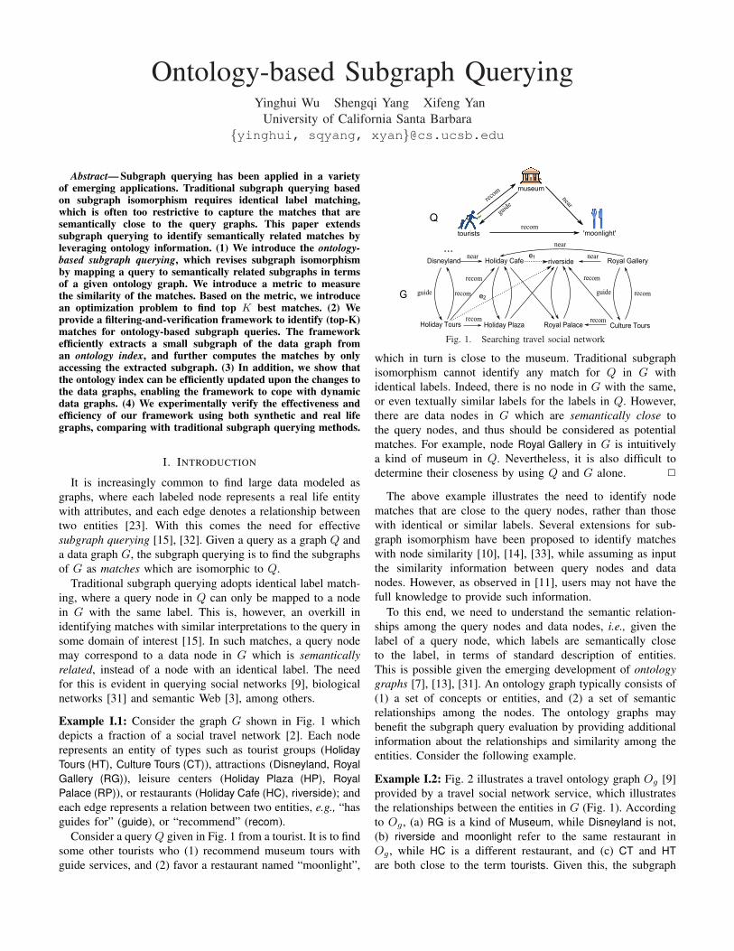
Example I.1: Consider the graph G shown in Fig. 1 whichdepicts a fraction of a social travel network [2]. Each noderepresents an entity of types such as tourist groups (HolidayTours (HT), Culture Tours (CT)), attractions (Disneyland, RoyalGallery (RG)), leisure centers (Holiday Plaza (HP), RoyalPalace (RP)), or restaurants (Holiday Cafe (HC), riverside); andeach edge represents a relation between two entities, e.g., “hasguides for” (guide), or “recommend” (recom).

Consider a query Q given in Fig. 1 from a tourist. It is to findsome other tourists who (1) recommend museum tours withguide services, and (2) favor a restaurant named “moonlight”,

museum

'moonlight'tourists

near

recom

guide

recomQ

Holiday Tours

Disneyland Holiday Cafe

Holiday Plaza Royal Palace

Royal Gallery

Culture Tours

riverside

guide guiderecom recomG

near

near near

recomrecom

recom

e1

e2

recom

...

Fig. 1. Searching travel social network

which in turn is close to the museum. Traditional subgraphisomorphism cannot identify any match for Q in G withidentical labels. Indeed, there is no node in G with the same,or even textually similar labels for the labels in Q. However,there are data nodes in G which are semantically close tothe query nodes, and thus should be considered as potentialmatches. For example, node Royal Gallery in G is intuitivelya kind of museum in Q. Nevertheless, it is also difficult todetermine their closeness by using Q and G alone. 2

The above example illustrates the need to identify nodematches that are close to the query nodes, rather than thosewith identical or similar labels. Several extensions for sub-graph isomorphism have been proposed to identify matcheswith node similarity [10], [14], [33], while assuming as inputthe similarity information between query nodes and datanodes. However, as observed in [11], users may not have thefull knowledge to provide such information.

To this end, we need to understand the semantic relation-ships among the query nodes and data nodes, i.e., given thelabel of a query node, which labels are semantically closeto the label, in terms of standard description of entities.This is possible given the emerging development of ontologygraphs [7], [13], [31]. An ontology graph typically consists of(1) a set of concepts or entities, and (2) a set of semanticrelationships among the nodes. The ontology graphs maybenefit the subgraph query evaluation by providing additionalinformation about the relationships and similarity among theentities. Consider the following example.

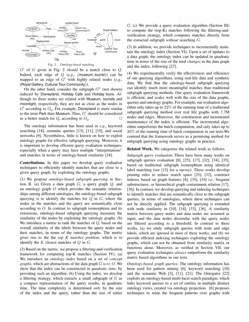
Example I.2: Fig. 2 illustrates a travel ontology graph Og [9]provided by a travel social network service, which illustratesthe relationships between the entities in G (Fig. 1). Accordingto Og , (a) RG is a kind of Museum, while Disneyland is not,(b) riverside and moonlight refer to the same restaurant inOg , while HC is a different restaurant, and (c) CT and HTare both close to the term tourists. Given this, the subgraph

museum

Royal Gallery

(RG)

Culture Tour

Community(CT)

Holiday

tours (HT)

guided tours

Disneyland

Park

leisure center

attractions

Restaurants

Holiday Cafe

(HC) Holiday

Plaza (HP) Royal

Palace (RP)

'riverside'

'moonlight

tourists

relocate

Royal Gallery

Culture Tour

Community

'riverside'

near

guide recom

recom

G'

Og

visit

...

Fig. 2. Ontology-based matching

G′ of G given in Fig. 2 should be a match close to Q.Indeed, each edge of Q (e.g., (museum, tourist)) can bemapped to an edge of G′ with highly related nodes (e.g.,(Royal Gallery, Cultural Tour Community)).

On the other hand, consider the subgraph G′′ (not shown)induced by Disneyland, Holiday Cafe and Holiday tours. Al-though its three nodes are related with Museum, tourists andmoonlight, respectively, they are not as close as the nodes inG′ according to Og . For example, Disneyland is more similarto the term Park than Museum. Thus, G′ should be consideredas a better match for Q, according to Og . 2

The ontology information has been used in e.g., keywordsearching [18], semantic queries [13], [11], [19], and socialnetworks [9]. Nevertheless, little is known on how to exploitontology graphs for effective subgraph querying. Moreover, itis important to develop efficient query evaluation techniques,especially when a query may have multiple “interpretations”and matches in terms of ontology-based similarity [18].

Contributions. In this paper we develop query evaluationtechniques to efficiently identify matches that are close to agiven query graph, by exploiting the ontology graphs.

(1) We propose ontology-based subgraph querying in Sec-tion II. (a) Given a data graph G, a query graph Q, andan ontology graph O which provides the semantic relation-ships among different ontologies, the ontology-based subgraphquerying is to identify the matches for Q in G, where thenodes in the matches and the query are semantically closeaccording to O. In contrast to subgraph isomorphism and itsextensions, ontology-based subgraph querying measures thesimilarity of the nodes by exploiting the ontology graphs. (b)We introduce a metric to rank the matches of Q, based on theoverall similarity of the labels between the query nodes andtheir matches, in terms of the ontology graphs. The metricgives rise to the the top K matches problem, which is toidentify the K closest matches of Q in G.

(2) Based on the metric, we propose a filtering-and-verificationframework for computing top-K matches (Section IV). (a)We introduce an ontology index based on a set of conceptgraphs, which are abstractions of the data graph G w.r.t. O. Weshow that the index can be constructed in quadratic time, byproviding such an algorithm. (b) Using the index, we developa filtering strategy, which extracts a small subgraph of G asa compact representation of the query results, in quadratictime. The time complexity is determined only by the sizeof the index and the query, rather than the size of entire

G. (c) We provide a query evaluation algorithm (Section III)to compute the (top-K) matches following the filtering-and-verification strategy, which computes matches directly fromthe extracted subgraph without searching G.

(3) In addition, we provide techniques to incrementally main-tain the ontology index (Section VI). Upon a set of updates toa data graph, the ontology index can be updated in quadratictime in terms of the size of the total changes in the data graphand the index, following [27].

(4) We experimentally verify the effectiveness and efficiencyof our querying algorithms, using real-life data and syntheticdata. We find that the ontology-based subgraph queryingcan identify much more meaningful matches than traditionalsubgraph querying methods. Our query evaluation frameworkis efficient, and scales well with the size of the data graphs,queries and ontology graphs. For example, our evaluation algo-rithm only takes up to 22% of the running time of a traditionalsubgraph querying method over real life graphs with 7.7Mnodes and edges. Moreover, the construction and incrementalmaintenance of the index is efficient. The incremental algo-rithm outperforms the batch computation, and only takes up to20% of the running time of batch computation in our tests.Wecontend that the framework serves as a promising method forsubgraph querying using ontology graphs in practice.

Related Work. We categorize the related work as follows.

Subgraph query evaluation. There have been many works onsubgraph queries evaluation [8], [25], [17], [32], [34], [35],based on traditional subgraph isomorphism using identicallabel matching (see [15] for a survey). These works developpruning rules to reduce search space [25], [32], constructindexes based on graph features [8], [35], [34] i.e., frequentsubstructures, or hierarchical graph containment relation [17],[36]. In contrast, we develop querying and indexing techniquesto identify matches that are semantically close to the subgraphqueries, in terms of ontologies, where these techniques cannot be directly applied. The subgraph querying is extendedwith node similarity in [10], [14], [33], [36]. A similaritymatrix between query nodes and data nodes are assumed asinput, and the data nodes dissimilar with the query nodesare filtered according to a threshold. In contrast to theseworks, (a) we study subgraph queries with node and edgelabels, which are ignored in most of these works; and (b) weprovide efficient indexing techniques exploiting the ontologygraphs, which can not be obtained from similarity matrix orfunctions alone. Moreover, as verified in Section VII, ourquery evaluation techniques always outperform the similaritymatrix based algorithms in our tests.

Ontology-based graph queries. The ontology information hasbeen used for pattern mining [6], keyword searching [18]and the semantic Web [3], [11], [21]. The Ontogator [22]exploits an ontology-based multi-facet search paradigm, whichlinks keyword queries to a set of entities in multiple distinctontology views, created via ontology projection. [6] proposestechniques to mine the frequent patterns over graphs with

generalized labels in the input taxonomies. Classes hierarchyare used to evaluate queries specified by a SPARQL-stylelanguage over RDF graphs in [11], where approximate answersare identified, measured by a distance metric. The templatematching with semantic similarity is discussed in [3], wherethe matches are semantically similar entities. However, thestructure of the template is not preserved, i.e., the matches arenot isomorphic to the template. Our work differs from theirsin the following. (a) We consider general ontology graphsrather than hierarchical taxonomies or class lattice. (b) Wefind matches for a given query graph, instead of discoveringfrequent patterns in graphs as in [6]. (c) The queries in [11]are defined in terms of a query language specified for semanticWeb. In contrast, we study general subgraph queries withnode and edge labels. Moreover, the queries in [11] are posedover RDF graphs with predefined schema, where we considersubgraph queries over general data graphs without any schema.(d) The query evaluation is not discussed in [3], [11], [21].

Closer to our work is [21], which extends template graphsearching by interpolating ontologies to data graphs. Thedata graphs are recursively extended by a set of ontologiesfrom ontology queries, and are then queried by a templategraph. Our work differs from theirs in (a) instead of mergingontology graphs with data graphs, we leverage ontology graphto develop filtering strategies to identify matches, and (b) weprovide query evaluation and indexing techniques, while [21]focus on data fusion techniques. The incremental queryingtechniques are also not addressed in [21].

Graph abstraction. The concepts of bisimulation [26] andregular equivalence [5] are proposed to define the equivalentgraph nodes, which can be grouped to form abstracted graphsas indexes [24]. In this work we use the similar idea toconstruct the ontology index, by abstracting data graphs asa set of concept graphs for efficient subgraph filtering andquerying. However, while the notions in [5], [26] are based onlabel equality, a concept graph groups nodes in a data graph interms of an external ontology graph, thus unifies the ontologysimilarity and graph abstraction, as discussed in Section IV.

II. ONTOLOGY-BASED SUBGRAPH QUERYING

Below we introduce data graphs and query graphs, as wellas the ontology graphs. We then introduce the notion of theontology-based subgraph querying.

A. Graphs, queries and ontology graphs

Data graph. A data graph is a directed graph G = (V, E, L),where V is a finite set of data nodes, E is the edge set where(u, u′) ∈ E denotes a data edge from node u to u′; and L is alabeling function which assigns a label L(v) (resp. L(e)) to anode v ∈ V (resp. an edge e ∈ E) In practice the function Lmay specify (1) the node labels as the description of entities,e.g., URL, location, name, job, age; and (2) the edge labelsas relationships between entities e.g., links, friendship, work,advice, support, exchange, co-membership [23].

pink rose

blue sky

flame

violet

green lime olive

red

rose pink flame

blue

sky

yellow

green

lime oliveviolet

Gc Ogc

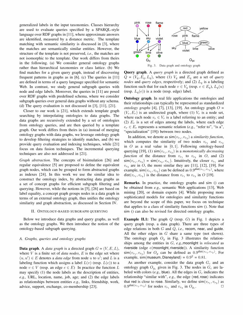
Fig. 3. Data graph and ontology graph

Query graph. A query graph is a directed graph defined asQ = (Vq, Eq, Lq), where (1) Vq and Eq are a set of querynodes and query edges, respectively; and (2) Lq is a labelingfunction such that for each node v ∈ Vq (resp. e ∈ Eq), Lq(u)(resp. Lq(e)) is a node (resp. edge) label.

Ontology graph. In real life applications the ontologies andtheir relationships can typically be represented as standardizedontology graphs [4], [7], [13], [19]. An ontology graph O =(Vr, Er) is an undirected graph, where (1) Vr is a node set,where each node vr ∈ Vr is a label referring to an entity; and(2) Er is a set of edges among the labels, where each edgeer ∈ Er represents a semantic relation (e.g., “refer to”, “is a”,“specialization” [19]) between two nodes.

In addition, we denote as sim(vr1 , vr2) a similarity function,which computes the similarity of two nodes vr1 and vr2

in O as a real value in [0, 1]. Following ontology-basedquerying [19], (1) sim(vr1 , vr2) is a monotonically decreasingfunction of the distance from vr1 to vr2 in O, and (2)sim(vr1 , vr2) = sim(vr2 , vr1). Intuitively, the closer vr1 andvr2 are in O, the more similar they are [11], [12], [19]. Forexample, sim(vr1 , vr2) can be defined as 0.9dist(vr1 ,vr2 ), wheredist(vr1 , vr2) is the distance from vr1 to vr2 in O [19].

Remarks. In practice, the ontology graphs and sim () canbe obtained from e.g., semantic Web applications [13], Webmining [20], or domain experts [4]. While proposing moresophisticated models for ontologies and similarity functionsare beyond the scope of this paper, we focus on techniquethat applies to a class of similarity functions sim (). Note thatsim () can also be revised for directed ontology graphs.

Example II.1: The graph Q (resp. G) in Fig. 1 depicts aquery graph (resp. a data graph). There are three types ofedge relations in both G and Q, i.e., recom, near, and guide.All the other edges in G share a same type (not shown).The ontology graph Og in Fig. 3 illustrates the relation-ships among the entities in G, e.g.,moonlight is relocated asriverside (edge e(moonlight, riverside)). A similarity functionsim(vr1 , vr2) for Og can be defined as 0.9dist(vr1 ,vr2 ). Forexample, sim(museum, Disneyland) = 0.92 = 0.81.

As another example, consider the data graph Gc and anontology graph Ogc given in Fig. 3. The nodes in Gc are la-beled with colors (e.g., blue). All the edges in Gc indicates therelationship “similar with”, e.g., the edge (red, rose) indicatesthat red is close to rose. Similarly, we define sim(vr1 , vr2) as0.9dist(vr1 ,vr2 ) for nodes vr1 and vr2 in Ogc

. 2

B. Ontology-based Subgraph Querying

We next introduce the ontology-based subgraph querying.Given a query graph Q = (Vq, Eq, Lq), an ontology graph

O, a data graph G = (V, E, L), a similarity function sim()and a similarity threshold θ, the ontology-based queryingis to find the subgraphs G′ = (V ′, E′, L′) of G, such thatthere is a bijective function h from Vq to V ′ where (a)sim(L(h(u)), Lq(u)) ≥ θ, and (b) (u, u′) is a query edge ifand only if(h(u), h(u′)) is a data edge, and they have the sameedge label. We refer to G′ as a match of Q in G induced by themapping h, and denote all the matches in G for Q as Q(G).In addition, the candidate set for a query node u as the set ofnodes v where sim(u, v) ≥ θ. Here we assume w.l.o.g. that allthe node labels in G are from O.

Top-K subgraph querying. In practice one often wants toidentify the matches that are semantically “closest” to a query.We present a quantitative metric for the overall similaritybetween a query graph Q and its match G′ induced by amapping h, defined by a function C as follows.

C(h) =∑

sim(Lq(u), L(h(u))), u ∈ Vq.

The metric favors the matches that are semantically closeto the query: the larger the similarity score C(h) is, the betterthe mapping is. On the other hand, if a subgraph G′ matchesQ with identical node labels, i.e., via a subgraph isomorphismmapping h, C(h) has the maximum value. Indeed, traditionalsubgraph isomorphism is a special case of the ontology-basedsubgraph querying, when the similarity threshold θ = 1.

The metric naturally gives rise to an optimization problem.Given Q, G, O and an integer K, the top K matches problemis to identify K matches for Q in G with the largest similarity.

Example II.2: Recall the query Q, the data graphG in Fig. 1 and the ontology graph Og in Fig. 2.Assume the similarity threshold θ = 0.9. One mayverify that the candidate set of query node museumcan(museum) = {Royal Gallery,attractions, park}, and sim-ilarly, can(moonlight) = {riverside, Holiday Cafe, HolidayPlaza}. The match G′ for Q in G has the maximum similar-ity sim(museum, Royal Gallery) + sim(tourists, Culture TourCommunity) + sim(moonlight, riverside) = 0.9 ∗ 3 = 2.7. 2

One may verify that the top K matches problem is NP-hard.Indeed, the traditional subgraph isomorphism is a special caseof the problem, which is known to be NP-complete [33]. Wenext provide a query evaluation framework for the problem.

III. QUERYING FRAMEWORK

Traditional ontology-based querying, by and large, relies onquery rewriting techniques [6], which replaces query nodeswith its candidates and may yield an exponential number ofqueries. These queries are then evaluated to produce all theresults. This may not be practical for ontology-based subgraphquerying. Alternatively, a similarity matrix can be computed,where each entry records the similarity between the querynodes and its candidates. Nevertheless, (1) the matrix incurs

Q

OgG

Index construction

concept graphs

filtering

verification

Q(G)

GoQ

Gv

Q

Q(Qv)

extracted

subgraph

Fig. 4. Ontology-based querying framework

high space and construction cost (O(|Q||G|)), and needs tobe computed upon each query, and (2) the time complexity isrelatively high for both the exact algorithms (e.g., [33]) andapproximation algorithms [14] over the entire data graph.

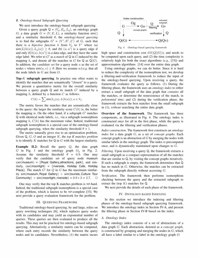
Using ontology graphs, we can do better. Since it is hardto reduce the complexity of the isomorphism test, we developa filtering-and-verification framework to reduce the input ofthe ontology-based querying. Upon receiving a query, theframework evaluates the query as follows. (1) During thefiltering phase, the framework uses an ontology index to eitherextract a small subgraph of the data graph that contains allthe matches, or determine the nonexistence of the match, inpolynomial time; and (2) during the verification phase, theframework extracts the best matches from the small subgraphin (1), without searching the entire data graph.

Overview of the framework. The framework has threecomponents, as illustrated in Fig. 4. The ontology index isconstructed once for all in the first phase, while the query isevaluated via the filtering and verification phases.

Index construction. The framework first constructs an ontologyindex for a data graph G, as a set of concept graphs. Eachconcept graph is an abstraction of G by merging the nodes withsimilar labels in the ontology graph. The index is precomputedonce, and is dynamically maintained upon changes to G.

Filtering. Upon receiving a query Q, the framework extracts asmall subgraph as a compact representation of all the matchesthat are similar to Q, by visiting the concept graphs iteratively.If such a subgraph is empty, the framework determines that Qhas no match in G. Otherwise, the matches can be extractedfrom the subgraph directly without accessing G.

Verification. The framework then performs isomorphismchecking between the query and the extracted subgraph toextract the (top K) matches for Q.

We next provide the details of each phase of the framework.

IV. ONTOLOGY-BASED INDEXING

In this section we introduce the indexing and filteringphases of the ontology-based subgraph querying framework.We introduce the ontology index in Section IV-A, and presentthe filtering phase in Section IV-B based on the index.

A. Ontology Index

The ontology index consists of a set of abstractions of adata graph G. Each abstraction, denoted as a concept graph,is constructed by grouping and merging the nodes in G, whichall have a label similar to a label in the ontology graph O.

pink rose

red

blue sky

blue

green lime

green

red(flame)

blue(violet)

green(olive)

G'c

museumtourists tpark

HP

RP

HC

riverside

Disneyland

RG

HT

CT

Go1

HP

HC

RP

riverside

Disneyland RGHT CT

Go2

leisure center moonlight

park park park

riversideleisure center

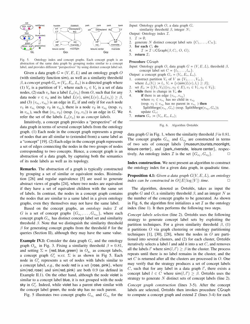
Fig. 5. Ontology index and concept graphs. Each concept graph is anabstraction of the same data graph by grouping nodes similar to a conceptlabel, and provides different “perspectives” by using distinct concept label set.

Given a data graph G = (V, E, L) and an ontology graph O(with similarity function sim), as well as a similarity thresholdβ, a concept graph Go = (Vo, Eo, Lo) is a directed graph where(1) Vo is a partition of V , where each vo ∈ Vo is a set of datanodes, (2) each vo has a label Lo(vo) from O, such that for anydata node v ∈ vo and its label L(v), sim(L(v), Lo(vo)) ≥ β,and (3) (vo1 , vo2) is an edge in Eo if and only if for each nodev1 in vo1 (resp. v2 in vo2), there is a node v2 in vo2 (resp. v1

in vo1), such that (v1, v2) (resp. (v2, v1)) is an edge in G. Werefer the set of the labels Lo(vo) to as concept labels.

Intuitively, a concept graph provides a “perspective” of thedata graph in terms of several concept labels from the ontologygraph. (1) Each node in the concept graph represents a groupof nodes that are all similar to (extended from) a same label asa “concept” [19]. (2) Each edge in the concept graph representsa set of edges connecting the nodes in the two groups of nodescorresponding to two concepts. Hence, a concept graph is anabstraction of a data graph, by capturing both the semanticsof its node labels as well as its topology.

Remarks. The abstraction of a graph is typically constructedby grouping a set of similar or equivalent nodes. Bisimula-tion [26] and regular equivalence [5] are used to generateabstract views of graphs [24], where two nodes are equivalentif they have a set of equivalent children with the same setof labels. In contrast, the nodes in a concept graph containsthe nodes that are similar to a same label in a given ontologygraphs, even they themselves may not have the same label.

Based on the concept graphs, an ontology index I ofG is a set of concept graphs {Go1 , . . . , Gom}, where eachconcept graph Goi has distinct concept label set and similaritythreshold β. Note that we distinguish the similarity thresholdβ for generating concept graphs from the threshold θ for thequeries (Section II), although they may have the same value.

Example IV.1: Consider the data graph Gc and the ontologygraph Ogc

in Fig. 3. Fixing a similarity threshold β = 0.81,and setting Σ = {red, blue, green} in Ogc

as concept labels,a concept graph G′c w.r.t. Σ is as shown in Fig 5. Eachnode in G′c represents a set of nodes with labels similar toa concept label, e.g., the node red is a set {rose, pink}, wheresim(red, rose) and sim(red, pink) are both 0.9 (as defined inExample II.1). On the other hand, although the node violet issimilar to a concept label blue, it is not grouped with the nodesky in G′c. Indeed, while violet has a parent olive similar withthe concept label green, the node sky has no such parent.

Fig. 5 illustrates two concept graphs Go1 and Go2 for the

Input: Ontology graph O, a data graph G,similarity threshold β, integer N ;

Output: Ontology index I.1. I := ∅;2. generate N distinct concept label sets {C1, . . . , CN};3. for each Ci do4. I := I ∪CGraph(β, Ci, O, G);5. return I;

Procedure CGraphInput: Ontology graph O, data graph G = (V, E, L), threshold β,

concept label set C = {l1, . . . , lm}.Output: a concept graph Go = (Vo, Eo, Lo).1. construct partition Vo of V as {V1, . . . , Vm},

where Lo(Vi) := li, Vi = {v|sim(L(v), li) ≥ β};2. set Eo := {(V1, V2)|(v1, v2 ∈ E), v1 ∈ V1, v2 ∈ V2};3. while there is change in Vo do4. if there is an edge (vo1 , vo2)

where v1 ∈ vo1 has no child in vo2

(resp. v2 ∈ vo2 has no parent in vo1 ) then5. SplitMerge(vo1 , Go) (resp. SplitMerge(vo2 , Go));6. update Go;7. return Go := (Vo, Eo, Lo);

Fig. 6. Algorithm OntoIdx

data graph G in Fig. 1, where the similarity threshold β is 0.81.The concept graphs Go1 and Go2 are constructed in termsof two sets of concept labels {museum,tourists,moonlight,leisure center}, and {park,,riverside, leisure center}, respec-tively. An ontology index I is the set {Go1 , Go2}. 2

Index construction. We next present an algorithm to constructthe ontology index for a given data graph, in quadratic time.

Proposition 4.1: Given a data graph G(V, E, L), an ontologyindex can be constructed in O(|E| log |V |) time. 2

The algorithm, denoted as OntoIdx, takes as input thegraphs G and O, a similarity threshold β, and an integer N asthe number of the concept graphs to be generated. As shownin Fig. 6, the algorithm first initializes a set I as the ontologyindex (line 1). It then performs the following two steps.

Concept labels selection (line 2). OntoIdx uses the followingstrategy to generate concept label sets by exploiting thepartition techniques. For a given similarity threshold β, (1)it partitions O via graph clustering or ontology partitioningtechniques [1], [30], [28], where the nodes in O are parti-tioned into several clusters, and (2) for each cluster, OntoIdxiteratively selects a label l and add it into a set C, and removesall the labels l′ where sim(l, l′) ≥ β in the cluster. The processrepeats until there is no label remains in the cluster, and theset C is returned after all the clusters are processed in O. Onemay verify that the strategy produces a set of concept labelsC, such that for any label in a data graph l′, there exists aconcept label l ∈ C where sim(l, l′) ≥ β. OntoIdx uses thestrategy to generate N distinct sets of concept labels (line 2).

Concept graph construction (lines 3-5). After the conceptlabels are selected, OntoIdx then invokes procedure CGraphto compute a concept graph and extend I (lines 3-4) for each

pink rose

blue sky

flame

violet

green lime olive

Gc0

red

blue

greengreen lime olive

pink rose

blue sky

flame

violet

red

blue

green lime

pink rose

blue sky

flame

blue(violet)

red

blue

Gc1 Gc2

green green

green(olive)

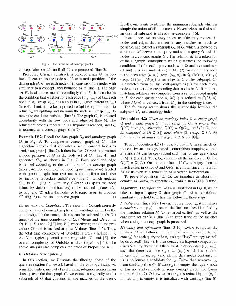
Fig. 7. Construction of concept graphs

concept label set Ci, until all Ci are processed (line 5).Procedure CGraph constructs a concept graph Go as fol-

lows. It constructs the node set Vo as a node partition of thedata graph G, where each node of Vo consists of the nodes withsimilarity to a concept label bounded by β (line 1). The edgeset Eo is also constructed accordingly (line 2). It then checksthe condition that whether for each edge (vo1 , vo2) of Go, eachnode in vo1 (resp. vo2) has a child in vo2 (resp. parent in vo1)(line 4). If not, it invokes a procedure SplitMerge (omitted) torefine Vo by splitting and merging the node vo1 (resp. vo2) tomake the condition satisfied (line 5). The graph Go is updatedaccordingly with the new node and edge set (line 6). Therefinement process repeats until a fixpoint is reached, and Go

is returned as a concept graph (line 7).

Example IV.2: Recall the data graph Gc and ontology graphOgc

in Fig. 3. To compute a concept graph of Gc, Thealgorithm OntoIdx first generates a set of concept labels as{red, blue, green} (line 2). It then invokes CGraph to constructa node partition of G as the node set of Gc (line 4), andgenerates Gc0 as shown in Fig. 7. Each node and edgeis refined according to the definition of the concept graph(lines 3-6). For example, the node (green, lime, olive) labeledwith green is split into two nodes (green, lime) and oliveby invoking procedure SplitMerge (line 5), which updatesGc0 to Gc1 (Fig 7). Similarly, CGraph (1) splits the node(blue, sky, violet) into (blue, sky) and violet, and updates Gc1

to Gc2 , and (2) splits the node (pink, rose, flame) to produceG′c (Fig. 5) as the final concept graph. 2

Correctness and Complexity. The algorithm CGraph correctlycomputes a set of concept graphs as the ontology index. For thecomplexity, (a) the concept labels can be selected in O(|O|)time; (b) the time complexity of SplitMerge and CGraph isO(|V |+|E|) and O(|E| log |V |), respectively; and (c) the pro-cedure CGraph is invoked at most N times (lines 4-5). Thus,the total time complexity of OntoIdx is O(N ∗ |E| log |V |).As N is typically small comparing with |V | and |E|, theoverall complexity of OntoIdx is thus O(|E| log |V |). Theabove analysis also completes the proof of Proposition 4.1.

B. Ontology-based filtering

In this section, we illustrate the filtering phase of thequery evaluation framework based on the ontology index. Asremarked earlier, instead of performing subgraph isomorphismdirectly over the data graph G, we extract a (typically small)subgraph of G that contains all the matches of the query.

Ideally, one wants to identify the minimum subgraph which issimply the union of all its matches. Nevertheless, to find suchan optimal subgraph is already NP-complete [16].

Instead, we use ontology index to efficiently reduce thenodes and edges that are not in any matches as much aspossible, and extract a subgraph Gv of G, which is induced bya relation M between the query nodes in a query Q and thenodes in a concept graphs Gc. The relation M is a relaxationof the subgraph isomorphism which guarantees the followingcondition: (1) for each query node u in Q and its matches v(if any), v is in a node M(u) in Gc, (2) for each query nodeu and each edge (u, u1) (resp. (u2, u)) in Q, (M(u),M(u1))(resp. (M(u2),M(u)) is an edge in Gc. The subgraph Gv

is extracted from Gc by “collapsing” M(u) for each querynode u to a set of corresponding data nodes in G. If multiplematching relations are computed from a set of concept graphsin I, for each query node u, M(u) is refined as

⋂Mi(u),

where Mi(u) is collected from Gci in the ontology index.The following result shows the relationship between the

subgraph Gv and ontology index.

Proposition 4.2: Given an ontology index I, a query graphQ and a data graph G, if the subgraph Gv is empty, thenQ(G) is empty; otherwise, Q(G) = Q(Gv), and (2) Gv canbe computed in O(|Q||I|) time, where |I| (resp. |Q|) is thetotal number of nodes and edges in I (resp. |Q|). 2

To see Proposition 4.2 (1), observe that if Q has a match G′

induced by an ontology-based isomorphism mapping h, thena relation M can be constructed such that for any query nodeu, h(u) ∈ M(u). Thus, Gv contains all the matches of Q, andQ(G) = Q(Gv). On the other hand, if Gv is empty, then nomatch exists in G for Q and Q(G) is empty, since no relationM exists even as a relaxation of subgraph isomorphism.

To prove Proposition 4.2 (2), we introduce an algorithm,denoted as Gview, to generate Gv from I in O(|Q||I|) time.

Algorithm. The algorithm Gview is illustrated in Fig. 8, whichtakes as input a query Q, data graph G and a user-definedsimilarity threshold θ. It has the following three steps.

Initialization (lines 1-2). For each query node vq, it initializesa match set mat(vq), to record the final matches identified bythe matching relation M (as remarked earlier), as well as thecandidate set can(vq) (line 2) to keep track of the matcheswhen a single concept graph is processed.

Matching and refinement (lines 3-10). Gview computes therelation M as follows. It first initializes the candidate setcan(vq) for each query node vq, using a “lazy” strategy (as willbe discussed) (line 4). It then conducts a fixpoint computation(lines 5-7), by checking if there exists a query edge (vq1 , vq2),such that there is a node vo1 ∈ can(vq1) which has no childin can(vq2). If so, vq1 (and all the data nodes contained init) is no longer a candidate for vq. Gview thus removes vq1

from can(vq1) (line 6). If can(vq1) is empty, then query nodeq1 has no valid candidate in some concept graph, and Gviewreturns ∅ (line 7). Otherwise, mat(vq1) is refined by can(vq1):if mat(vq1) is empty, it is initialized with can(vq1) (line 8);

Input: query Q = (Vq, Eq, Lq), ontology index I,similarity threshold θ;

Output: a subgraph Gv .1. set Vqv := ∅, Eqv := ∅;2. for each vq ∈ Vq do set mat(vq) := ∅; can(vq) := ∅;3. for each Go ∈ I do4. for each vq ∈ Vq do compute can(vq) with lazy strategy;5. while there is an edge (vq1 , vq2) ∈ Eq and vo1 ∈ can(vq1)

such that C(vo1, Go) ∩ can(vq2) = ∅ then6. can(vq1) := can(vq1) \ {vo1};7. if can(vq1) = ∅ then return ∅;8. if mat(vq) = ∅ then mat(vq) := can(vq);9. else mat(vq) := mat(vq) ∩ can(vq);10. if mat(vq) = ∅ then return ∅;11. for each vq ∈ Vq do12. construct Vqv and Eqv with mat(vq) and Go;13. construct Gv:= (Vqv , Eqv , Lqv );14. return Gv;

Fig. 8. Algorithm Gview

otherwise, mat(vq1) only keeps those candidates that are incan(vq1) (line 9). If mat(vq1) becomes empty, no candidatecan be find in G for vq1 , and Gview returns ∅ (line 10).

Gv construction (lines 11-14). After all the concept graphsin I are processed, Gview constructs Gv with a node set Vqv ,which contains a node for each match set, and a correspondingedge set Eqv

(lines 11-13). Gv is then returned (lines 14).It is costly to identify the candidates for the query nodes in

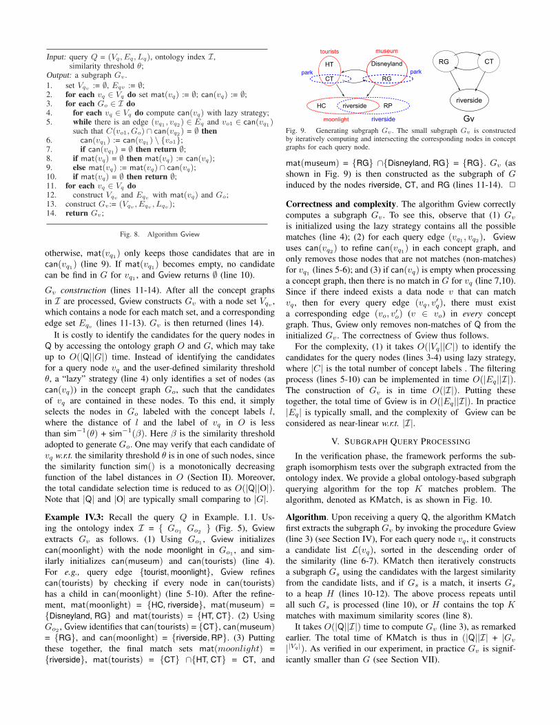
Q by accessing the ontology graph O and G, which may takeup to O(|Q||G|) time. Instead of identifying the candidatesfor a query node vq and the user-defined similarity thresholdθ, a “lazy” strategy (line 4) only identifies a set of nodes (ascan(vq)) in the concept graph Go, such that the candidatesof vq are contained in these nodes. To this end, it simplyselects the nodes in Go labeled with the concept labels l,where the distance of l and the label of vq in O is lessthan sim−1(θ) + sim−1(β). Here β is the similarity thresholdadopted to generate Go. One may verify that each candidate ofvq w.r.t. the similarity threshold θ is in one of such nodes, sincethe similarity function sim() is a monotonically decreasingfunction of the label distances in O (Section II). Moreover,the total candidate selection time is reduced to as O(|Q||O|).Note that |Q| and |O| are typically small comparing to |G|.Example IV.3: Recall the query Q in Example. I.1. Us-ing the ontology index I = { Go1 Go2 } (Fig. 5), Gviewextracts Gv as follows. (1) Using Go1 , Gview initializescan(moonlight) with the node moonlight in Go1 , and sim-ilarly initializes can(museum) and can(tourists) (line 4).For e.g., query edge {tourist, moonlight}, Gview refinescan(tourists) by checking if every node in can(tourists)has a child in can(moonlight) (line 5-10). After the refine-ment, mat(moonlight) = {HC, riverside}, mat(museum) ={Disneyland, RG} and mat(tourists) = {HT, CT}. (2) UsingGo2 , Gview identifies that can(tourists) = {CT}, can(museum)= {RG}, and can(moonlight) = {riverside, RP}. (3) Puttingthese together, the final match sets mat(moonlight) ={riverside}, mat(tourists) = {CT} ∩{HT, CT} = CT, and

tourists

HT

CT

museum

Disneyland

RG

HC riverside

moonlight

RPriverside

RG CT

Gv

park park

riverside

Fig. 9. Generating subgraph Gv . The small subgraph Gv is constructedby iteratively computing and intersecting the corresponding nodes in conceptgraphs for each query node.

mat(museum) = {RG} ∩{Disneyland, RG} = {RG}. Gv (asshown in Fig. 9) is then constructed as the subgraph of Ginduced by the nodes riverside, CT, and RG (lines 11-14). 2

Correctness and complexity. The algorithm Gview correctlycomputes a subgraph Gv . To see this, observe that (1) Gv

is initialized using the lazy strategy contains all the possiblematches (line 4); (2) for each query edge (vq1 , vq2), Gviewuses can(vq2) to refine can(vq1) in each concept graph, andonly removes those nodes that are not matches (non-matches)for vq1 (lines 5-6); and (3) if can(vq) is empty when processinga concept graph, then there is no match in G for vq (line 7,10).Since if there indeed exists a data node v that can matchvq, then for every query edge (vq, v

′q), there must exist

a corresponding edge (vo, v′o) (v ∈ vo) in every concept

graph. Thus, Gview only removes non-matches of Q from theinitialized Gv . The correctness of Gview thus follows.

For the complexity, (1) it takes O(|Vq||C|) to identify thecandidates for the query nodes (lines 3-4) using lazy strategy,where |C| is the total number of concept labels . The filteringprocess (lines 5-10) can be implemented in time O(|Eq||I|).The construction of Gv is in time O(|I|). Putting thesetogether, the total time of Gview is in O(|Eq||I|). In practice|Eq| is typically small, and the complexity of Gview can beconsidered as near-linear w.r.t. |I|.

V. SUBGRAPH QUERY PROCESSING

In the verification phase, the framework performs the sub-graph isomorphism tests over the subgraph extracted from theontology index. We provide a global ontology-based subgraphquerying algorithm for the top K matches problem. Thealgorithm, denoted as KMatch, is as shown in Fig. 10.

Algorithm. Upon receiving a query Q, the algorithm KMatchfirst extracts the subgraph Gv by invoking the procedure Gview(line 3) (see Section IV), For each query node vq, it constructsa candidate list L(vq), sorted in the descending order ofthe similarity (line 6-7). KMatch then iteratively constructsa subgraph Gs using the candidates with the largest similarityfrom the candidate lists, and if Gs is a match, it inserts Gs

to a heap H (lines 10-12). The above process repeats untilall such Gs is processed (line 10), or H contains the top Kmatches with maximum similarity scores (line 8).

It takes O(|Q||I|) time to compute Gv (line 3), as remarkedearlier. The total time of KMatch is thus in (|Q||I| + |Gv

||Vq|). As verified in our experiment, in practice Gv is signif-icantly smaller than G (see Section VII).

Input: query Q = (Vq, Eq, Lq), ontology graph O,ontology index I, data graph G;

Output: a set of top-K matches for Q in G w.r.t. O.1. set Match = ∅;2. /* filtering */3. extract a subgraph Gv:= Gview(Q, I);4. /* verification */5. heap H = ∅;6. for each vq ∈ Vq do7. construct a sorted candidate node list L(vq) in Gv;8. while |H| ≤ K do9. construct a distinct node list L′ with L() maximizing

the overall similarity;10. if L′ = ∅ then break ;11. construct Gs induced by the data nodes in L′;12. if Gs is a match of Q then insert Gs to H;13. return H;

Fig. 10. Algorithm KMatch

Remarks. The ontology-based subgraph querying frameworkcan be easily adapted to support traditional subgraph isomor-phism. Indeed, when the user-defined similarity threshold is1.0, (1) the ontology index can be used to extract a subgraphGv , which only contains the candidate nodes with identicallabels for the query nodes, and (2) any match extracted fromGv is a subgraph isomorphic to Q in terms of identicalsubgraph isomorphism.

VI. ONTOLOGY INDEX MAINTENANCE

The ontology-based subgraph querying framework can ef-ficiently extracts a compact subgraph of a data graph fromthe ontology index, which is then queried for verification andresults generation. In practice the data graphs are changingfrequently over time. In this section we investigate the in-cremental maintenance of the ontology index, which furtherenables the ontology-based subgraph querying to cope withdynamic data graphs. Indeed, a dynamic subgraph queryingframework can be readily developed by incrementally updat-ing the ontology index, and then performs the filtering andverification phases to compute the new matches.

Given a set of updates ∆G to the data graph G, and anontology index I, the index maintenance is to update I to anontology index for the updated data graph G ⊕ ∆G. Insteadof recomputing the concept graphs from scratch each time thedata graph is updated, we show that the index I can be directlyupdated by only accessing ∆G.

As observed in [27], it is no longer adequate to measure thecomplexity of incremental algorithms by using the traditionalcomplexity analysis for batch algorithms. Following [27], wecharacterize the complexity of an incremental graph algorithmin terms of the size of the affected area (AFF), which indicatesthe changes in the input ∆G and the ∆I, i.e., |AFF| = |∆G|+ |∆I|. Specifically, ∆I contains the nodes and edges thatare not shared by I and I ′ as the updated I.

Proposition 6.1: Given a data graph G and a set of updates∆G (edge insertions and deletions), the ontology index I canbe maintained in O(|AFF|2 + |I|) time. 2

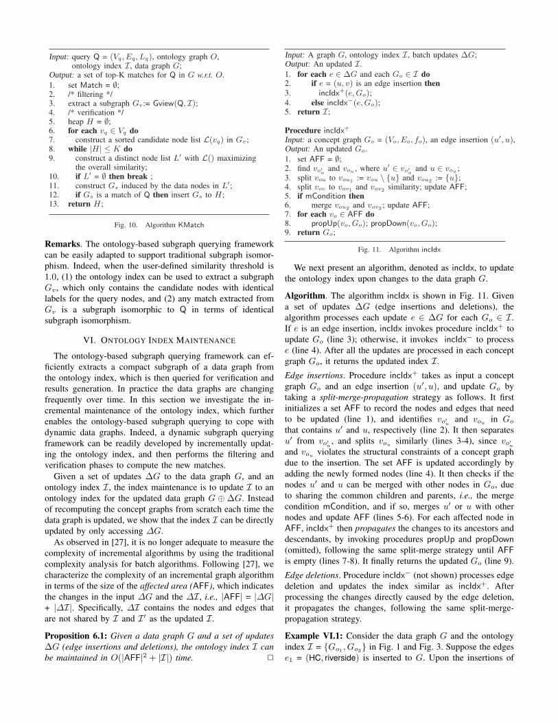
Input: A graph G, ontology index I, batch updates ∆G;Output: An updated I.1. for each e ∈ ∆G and each Go ∈ I do2. if e = (u, v) is an edge insertion then3. incIdx+(e, Go);4. else incIdx−(e, Go);5. return I;

Procedure incIdx+

Input: a concept graph Go = (Vo, Eo, fo), an edge insertion (u′, u),Output: An updated Go.1. set AFF = ∅;2. find vo′u and vou , where u′ ∈ vo′u and u ∈ vou ;3. split vou to vou1 := vou \ {u} and vou2 := {u};4. split vov to vov1 and vov2 similarity; update AFF;5. if mCondition then6. merge vou2 and vov2 ; update AFF;7. for each vo ∈ AFF do8. propUp(vo, Go); propDown(vo, Go);9. return Go;

Fig. 11. Algorithm incIdx

We next present an algorithm, denoted as incIdx, to updatethe ontology index upon changes to the data graph G.

Algorithm. The algorithm incIdx is shown in Fig. 11. Givena set of updates ∆G (edge insertions and deletions), thealgorithm processes each update e ∈ ∆G for each Go ∈ I.If e is an edge insertion, incIdx invokes procedure incIdx+ toupdate Go (line 3); otherwise, it invokes incIdx− to processe (line 4). After all the updates are processed in each conceptgraph Go, it returns the updated index I.

Edge insertions. Procedure incIdx+ takes as input a conceptgraph Go and an edge insertion (u′, u), and update Go bytaking a split-merge-propagation strategy as follows. It firstinitializes a set AFF to record the nodes and edges that needto be updated (line 1), and identifies vo′u and vou

in Go

that contains u′ and u, respectively (line 2). It then separatesu′ from vo′u , and splits vou

similarly (lines 3-4), since vo′uand vou

violates the structural constraints of a concept graphdue to the insertion. The set AFF is updated accordingly byadding the newly formed nodes (line 4). It then checks if thenodes u′ and u can be merged with other nodes in Go, dueto sharing the common children and parents, i.e., the mergecondition mCondition, and if so, merges u′ or u with othernodes and update AFF (lines 5-6). For each affected node inAFF, incIdx+ then propagates the changes to its ancestors anddescendants, by invoking procedures propUp and propDown(omitted), following the same split-merge strategy until AFFis empty (lines 7-8). It finally returns the updated Go (line 9).

Edge deletions. Procedure incIdx− (not shown) processes edgedeletion and updates the index similar as incIdx+. Afterprocessing the changes directly caused by the edge deletion,it propagates the changes, following the same split-merge-propagation strategy.

Example VI.1: Consider the data graph G and the ontologyindex I = {Go1 , Go2} in Fig. 1 and Fig. 3. Suppose the edgese1 = (HC, riverside) is inserted to G. Upon the insertions of

e1, incIdx splits the node {HC, riverside} into {HC} and{riverside}, which are added to AFF (lines 3-4). It thenpropagates the changes and splits the node {HP, RP} in Go1 .The updated concept graph G′o1

contains six nodes, with twonewly separated nodes as remarked earlier. On the other hand,no change is incurred to Go2 . The updated I thus contains G′o1

and Go2 . The total AFF includes the nodes {HC, riverside},{HP, RP} in Go1 , and the newly separated nodes in G′o1

.Now suppose edge e2 = (HT, riverside) is inserted into

G. Similarly, one may verify that the insertion of e2, whiledoes not affect Go1 , changes Go2 by splitting its node{RP, riverside}. The affected area AFF includes the node{RP, riverside} and the two nodes RP and riverside. 2

Analysis. One may verify that both incIdx+ and incIdx− pre-serve the following invariants: each split, merge and propagateoperation do not introduce nodes and edges that violates thenode and topological constraints of concept graphs. Thecorrectness of incIdx thus follows. The complexity of incIdxis in O(|AFF|2 + |I|). To see this, for incIdx+, it takes O(|I|)time to perform the split and merge operation, and the propaga-tion propUp and propDown takes O(|AFF|2) time as fixpointcomputation. Similarly, the complexity of procedureincIdx−

is in O(|AFF|2 + |I|). Thus, the total complexity of incIdx isin O(|AFF|2 + |I|). As verified in our experiments, |AFF| istypically small and the index can be efficiently updated.

VII. EXPERIMENTAL EVALUATION

We next present an experimental study using both real-lifeand synthetic data. We conducted three sets of experiments toevaluate: (1) the effectiveness of the ontology-based subgraphquerying, (2) the efficiency of the query evaluation framework,and (3) the performance and cost of the ontology index.

Datasets. We used the following datasets.

(1) Real-life graphs. We used the following two real-lifedatasets, each consists of a data graph and an ontologygraph. (a) CrossDomain is taken from a benchmark suiteFebBench [29], which consists of (i) an RDF data graph with1.07M nodes and 3.86M edges where nodes represent entitiesfrom different domains (e.g., Wikipedia, locations, biology,music, newspapers), and edges represent the relationship be-tween the entities (e.g., born in, locate at, favors); and (ii) anontology graph with 1.44M concepts and 5.30M relations. Thedata graph takes in total 150Mb physical memory. (b) Flickrcontains a data graph taken from http://press.liacs.nl/mirflickr/ with 1.3M nodes and 6.42M edges, wherethe nodes represent images, tags, users or locations, and edgesrepresent their relationship. It also contains an ontology graphfrom DBpedia (http://dbpedia.org) with more than3.64 million entities. The data graph takes in total 194Mbphysical memory. In our experiments, we employ the ontologygraph to describe the tags in Flickr.

(2) Synthetic data. We designed a graph generator to producerandomly generated synthetic graphs, which was controlledby three parameters: the number of nodes |V |, the number

of edges |E|, and the size |L| of the node label set. Wealso generate ontology graphs for the set of synthetic graphssharing the same set of label L, controlled by the same setof parameters. We use (|V |, |E|) to denote the size of a datagraph, and the ontology graph.

Following [19], we set the similarity function as sim(l′, l)= 0.9dist(l′,l) for all the ontology graphs O, where dist(l′, l) isthe distance between two nodes l′ and l in O. For example, ifa label l is 2 hops away from l′ in O, sim(l′, l) = 0.81.

Implementation. We implemented the following algorithmsin C++: (1) algorithm OntoIdx; (2) algorithm KMatch; (3)SubIso, the subgraph isomorphism algorithm in [32], whichidentifies the matches using identical label matching; (4)SubIsor, which, as a comparison to KMatch, is revisedfrom [32] that rewrites the query graph, and directly computesall the matches and select the best ones; (4) VF2, whichcomputes the minimum weighted matches, by exploiting asimilarity matrix between the query label and all the labelsin the data nodes; (4) our incremental algorithm incIdx.

To favor VF2, we precomputed a similarity matrix, whereeach entry records sim(u, v) as the similarity between a querynode u and a data node v w.r.t. the ontology graph O. Wealso optimized VF2 such that it terminates as soon as the topK matches are identified. The time cost of computing thesimilarity matrix is not counted for VF2.

We used a machine powered by an Intel(R) Core 2.8GHzCPU and 8GB of RAM, using Ubuntu 10.10. Each experimentwas run 5 times and the average is reported here.

Experimental results. We next present our findings.

Exp-1: Effectiveness and flexibility. In this set of ex-periments, we first evaluated the effectiveness of KMatchand SubIso. We generated 5 query templates for CrossDomain,and 4 query templates for Flickr. We use (|Vp|, |Ep|, |Lp|) todenote the size of a query Q(Vp, Ep, Lp). For CrossDomain,(1) QT1 is a tree of size (4, 3, 3) searching for movies, directorsand distributors, and QT2 of size (4, 4, 3) is a cycle obtainedby inserting an edge to QT1 ; (2) QT3 of size (4, 6, 4) is tosearch pop stars, record companies, albums and songs, andQ4 is obtained by only “generalizing” the query label of QT3 ,e.g., from “Green Record Company” to “Record Company”;and (3) QT5 of size (5, 6, 4) is to identify the soccer stars,clubs and their teammates. Similarly, for Flickr the 4 queriesQT6 to QT9 are to identify photos of animals taken at specifiedlocations. Each template QTi

is populated as a query set of100 queries (also denoted as QTi

) by varying the node labelsonly. For ontology index, we employ the graph partitioningalgorithm in [28] to generate concept labels with similaritythreshold β = 0.8, unless otherwise specified.

Effectiveness. We first compared the number of matches foundby SubIso and KMatch over CrossDomain and Flickr, asshown in Table I. Fixing card I = 1, i.e., the ontology index(I) contains a single concept graph, we varied the similaritythreshold of the queries from 1.0 to 0.8, and identify all thematches. For all the queries over CrossDomain, SubIso only

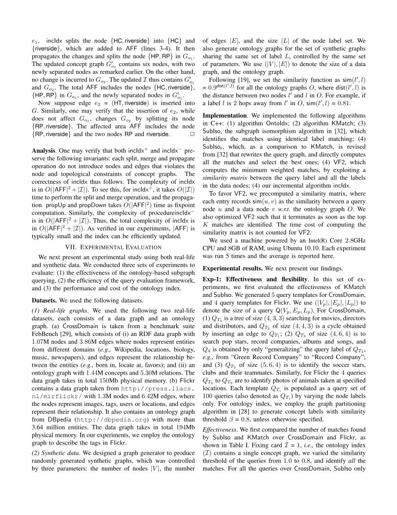
CrossDomainQueryθ=1θ=0.9 θ=0.8

QT1 1 2,687 9,099QT2 0 24 271QT3 1 170 342QT4 0 405 991QT5 0 30,854 48,225

FlickrQueryθ=1θ=0.9θ=0.8

QT6 2 6 307QT7 0 177 2,160QT8 0 448 6,028QT9 0 799 15,052

TABLE IEFFECTIVENESS OVER REAL LIFE GRAPHS

finds in average 1 exact match for query set QT1 and QT3 , andno match for all other queries. In contrast, KMatch identifiesmuch more matches that are semantically close to the queryaccording to our observation. It also finds more meaningfulmatches than SubIso over Flickr.

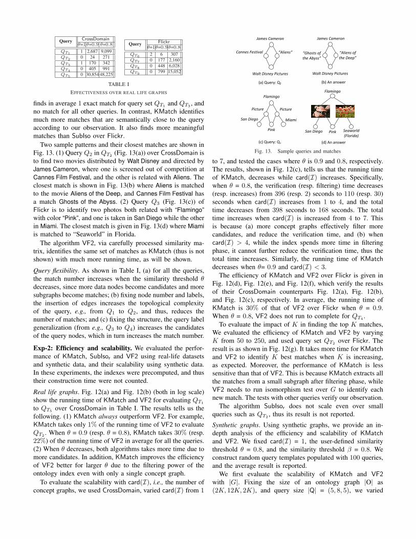
Two sample patterns and their closest matches are shown inFig. 13. (1) Query Q2 in QT2 (Fig. 13(a)) over CrossDomain isto find two movies distributed by Walt Disney and directed byJames Cameron, where one is screened out of competition atCannes Film Festival, and the other is related with Aliens. Theclosest match is shown in Fig. 13(b) where Aliens is matchedto the movie Aliens of the Deep, and Cannes Film Festival hasa match Ghosts of the Abyss. (2) Query Q3 (Fig. 13(c)) ofFlickr is to identify two photos both related with “Flamingo”with color “Pink”, and one is taken in San Diego while the otherin Miami. The closest match is given in Fig. 13(d) where Miamiis matched to “Seaworld” in Florida.

The algorithm VF2, via carefully processed similarity ma-trix, identifies the same set of matches as KMatch (thus is notshown) with much more running time, as will be shown.

Query flexibility. As shown in Table I, (a) for all the queries,the match number increases when the similarity threshold θdecreases, since more data nodes become candidates and moresubgraphs become matches; (b) fixing node number and labels,the insertion of edges increases the topological complexityof the query, e.g., from Q1 to Q2, and thus, reduces thenumber of matches; and (c) fixing the structure, the query labelgeneralization (from e.g., Q3 to Q4) increases the candidatesof the query nodes, which in turn increases the match number.

Exp-2: Efficiency and scalability. We evaluated the perfor-mance of KMatch, SubIsor and VF2 using real-life datasetsand synthetic data, and their scalability using synthetic data.In these experiments, the indexes were precomputed, and thustheir construction time were not counted.

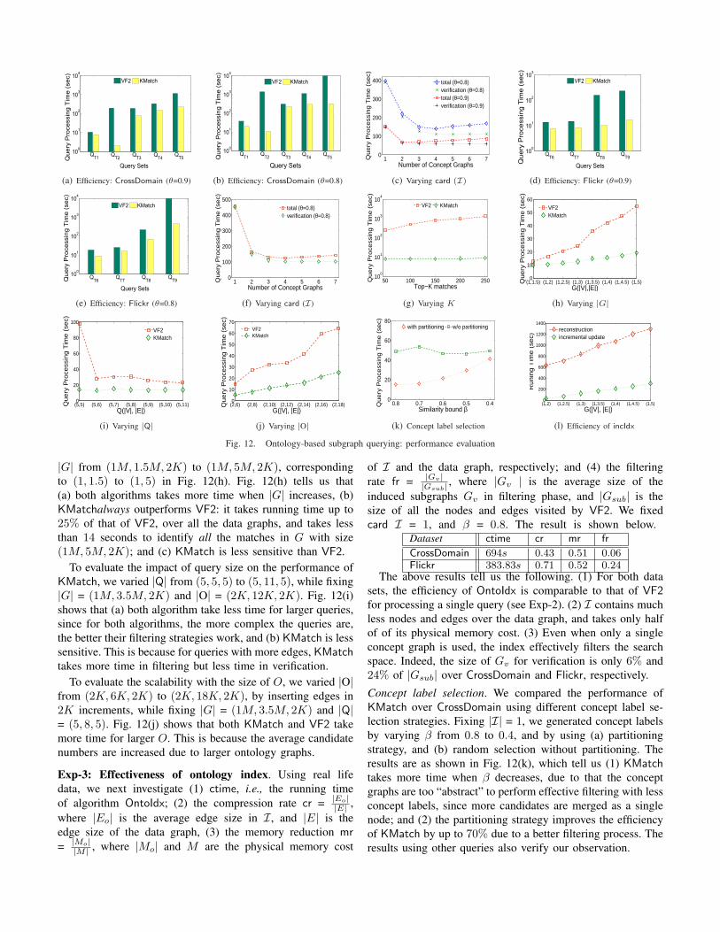
Real life graphs. Fig. 12(a) and Fig. 12(b) (both in log scale)show the running time of KMatch and VF2 for evaluating QT1

to QT5 over CrossDomain in Table I. The results tells us thefollowing. (1) KMatch always outperform VF2. For example,KMatch takes only 1% of the running time of VF2 to evaluateQT2 . When θ = 0.9 (resp. θ = 0.8), KMatch takes 30% (resp.22%) of the running time of VF2 in average for all the queries.(2) When θ decreases, both algorithms takes more time due tomore candidates. In addition, KMatch improves the efficiencyof VF2 better for larger θ due to the filtering power of theontology index even with only a single concept graph.

To evaluate the scalability with card(I), i.e., the number ofconcept graphs, we used CrossDomain, varied card(I) from 1

(c) Query: Q3San Diego Miami

(d) An answer

Flamingo

Pink San Diego Seaworld (Florida)

Flamingo

Pink

Picture Picture

(a) Query: Q2

James Cameron

“Aliens”Cannes Festival

Walt Disney Pictures

James Cameron

“Ghosts of the Abyss”

“Aliens of the Deep”

Walt Disney Pictures(b) An answer

Fig. 13. Sample queries and matches

to 7, and tested the cases where θ is 0.9 and 0.8, respectively.The results, shown in Fig. 12(c), tells us that the running timeof KMatch, decreases while card(I) increases. Specifically,when θ = 0.8, the verification (resp. filtering) time decreases(resp. increases) from 396 (resp. 2) seconds to 110 (resp. 30)seconds when card(I) increases from 1 to 4, and the totaltime decreases from 398 seconds to 168 seconds. The totaltime increases when card(I) is increased from 4 to 7. Thisis because (a) more concept graphs effectively filter morecandidates, and reduce the verification time, and (b) whencard(I) > 4, while the index spends more time in filteringphase, it cannot further reduce the verification time, thus thetotal time increases. Similarly, the running time of KMatchdecreases when θ= 0.9 and card(I) < 3.

The efficiency of KMatch and VF2 over Flickr is given inFig. 12(d), Fig. 12(e), and Fig. 12(f), which verify the resultsof their CrossDomain counterparts Fig. 12(a), Fig. 12(b),and Fig. 12(c), respectively. In average, the running time ofKMatch is 30% of that of VF2 over Flickr when θ = 0.9.When θ = 0.8, VF2 does not run to complete for QT4 .

To evaluate the impact of K in finding the top K matches,We evaluated the efficiency of KMatch and VF2 by varyingK from 50 to 250, and used query set QT2 over Flickr. Theresult is as shown in Fig. 12(g). It takes more time for KMatchand VF2 to identify K best matches when K is increasing,as expected. Moreover, the performance of KMatch is lesssensitive than that of VF2. This is because KMatch extracts allthe matches from a small subgraph after filtering phase, whileVF2 needs to run isomorphism test over G to identify eachnew match. The tests with other queries verify our observation.

The algorithm SubIsor does not scale even over smallqueries such as QT2 , thus its result is not reported.

Synthetic graphs. Using synthetic graphs, we provide an in-depth analysis of the efficiency and scalability of KMatchand VF2. We fixed card(I) = 1, the user-defined similaritythreshold θ = 0.8, and the similarity threshold β = 0.8. Weconstruct random query templates populated with 100 queries,and the average result is reported.

We first evaluate the scalability of KMatch and VF2with |G|. Fixing the size of an ontology graph |O| as(2K, 12K, 2K), and query size |Q| = (5, 8, 5), we varied

100

101

102

103

104

Query

Pro

cessin

g T

ime (

sec)

VF2 KMatch

QT1

QT2

QT3

QT4

QT5

Query Sets

(a) Efficiency: CrossDomain (θ=0.9)

100

101

102

103

104

Qu

ery

Pro

ce

ssin

g T

ime (

se

c)

VF2 KMatch

QT1

QT2

QT3

QT4

QT5

Query Sets

(b) Efficiency: CrossDomain (θ=0.8)

1 2 3 4 5 6 70

100

200

300

400

Number of Concept Graphs

Qu

ery

Pro

cess

ing

Tim

e (

sec)

total (θ=0.8)verification (θ=0.8)total (θ=0.9)verification (θ=0.9)

(c) Varying card (I)

100

101

102

103

Query

Pro

cessin

g T

ime (

sec)

VF2 KMatch

QT7

QT8

QT9

QT6

Query Sets

(d) Efficiency: Flickr (θ=0.9)

100

101

102

103

104

Qu

ery

Pro

ce

ssin

g T

ime (

se

c)

VF2 KMatch

QT6

QT7

QT8

QT9

Query Sets

(e) Efficiency: Flickr (θ=0.8)

1 2 3 4 5 6 70

100

200

300

400

500

Number of Concept Graphs

Qu

ery

Pro

cess

ing

Tim

e (

sec)

total (θ=0.8)verification (θ=0.8)

(f) Varying card (I)

50 100 150 200 25010

0

101

102

103

104

Top−K matches

Qu

ery

Pro

cess

ing

Tim

e (

sec)

VF2 KMatch

(g) Varying K

(1,1.5) (1,2) (1,2.5) (1,3) (1,3.5) (1,4) (1,4.5) (1,5)0

10

20

30

40

50

60

G(|V|,|E|)

Query

Pro

cess

ing T

ime (

sec)

VF2KMatch

(h) Varying |G|

(5,5) (5,6) (5,7) (5,8) (5,9) (5,10) (5,11)0

20

40

60

80

100

Q(|V|, |E|)

Query

Pro

cess

ing T

ime (

sec)

VF2KMatch

(i) Varying |Q|

(2,6) (2,8) (2,10) (2,12) (2,14) (2,16) (2,18)0

10

20

30

40

50

60

70

G(|V|, |E|)

Query

Pro

cess

ing T

ime (

sec)

VF2KMatch

(j) Varying |O|

0.8 0.7 0.6 0.5 0.40

20

40

60

80

Similarity bound β

Qu

ery

Pro

cess

ing

Tim

e (

sec)

with partitioning w/o partitioning

(k) Concept label selection

(1,2) (1,2.5) (1,3) (1,3.5) (1,4) (1,4.5) (1,5)0

200

400

600

800

1000

1200

1400

G(|V|, |E|)

Runin

g T

ime (

sec)

reconstructionincremental update

(l) Efficiency of incIdx

Fig. 12. Ontology-based subgraph querying: performance evaluation

|G| from (1M, 1.5M, 2K) to (1M, 5M, 2K), correspondingto (1, 1.5) to (1, 5) in Fig. 12(h). Fig. 12(h) tells us that(a) both algorithms takes more time when |G| increases, (b)KMatchalways outperforms VF2: it takes running time up to25% of that of VF2, over all the data graphs, and takes lessthan 14 seconds to identify all the matches in G with size(1M, 5M, 2K); and (c) KMatch is less sensitive than VF2.

To evaluate the impact of query size on the performance ofKMatch, we varied |Q| from (5, 5, 5) to (5, 11, 5), while fixing|G| = (1M, 3.5M, 2K) and |O| = (2K, 12K, 2K). Fig. 12(i)shows that (a) both algorithm take less time for larger queries,since for both algorithms, the more complex the queries are,the better their filtering strategies work, and (b) KMatch is lesssensitive. This is because for queries with more edges, KMatchtakes more time in filtering but less time in verification.

To evaluate the scalability with the size of O, we varied |O|from (2K, 6K, 2K) to (2K, 18K, 2K), by inserting edges in2K increments, while fixing |G| = (1M, 3.5M, 2K) and |Q|= (5, 8, 5). Fig. 12(j) shows that both KMatch and VF2 takemore time for larger O. This is because the average candidatenumbers are increased due to larger ontology graphs.

Exp-3: Effectiveness of ontology index. Using real lifedata, we next investigate (1) ctime, i.e., the running timeof algorithm OntoIdx; (2) the compression rate cr = |Eo|

|E| ,where |Eo| is the average edge size in I, and |E| is theedge size of the data graph, (3) the memory reduction mr= |Mo|

|M | , where |Mo| and M are the physical memory cost

of I and the data graph, respectively; and (4) the filteringrate fr = |Gv|

|Gsub| , where |Gv | is the average size of theinduced subgraphs Gv in filtering phase, and |Gsub| is thesize of all the nodes and edges visited by VF2. We fixedcard I = 1, and β = 0.8. The result is shown below.

Dataset ctime cr mr fr

CrossDomain 694s 0.43 0.51 0.06Flickr 383.83s 0.71 0.52 0.24

The above results tell us the following. (1) For both datasets, the efficiency of OntoIdx is comparable to that of VF2for processing a single query (see Exp-2). (2) I contains muchless nodes and edges over the data graph, and takes only halfof of its physical memory cost. (3) Even when only a singleconcept graph is used, the index effectively filters the searchspace. Indeed, the size of Gv for verification is only 6% and24% of |Gsub| over CrossDomain and Flickr, respectively.

Concept label selection. We compared the performance ofKMatch over CrossDomain using different concept label se-lection strategies. Fixing |I| = 1, we generated concept labelsby varying β from 0.8 to 0.4, and by using (a) partitioningstrategy, and (b) random selection without partitioning. Theresults are as shown in Fig. 12(k), which tell us (1) KMatchtakes more time when β decreases, due to that the conceptgraphs are too “abstract” to perform effective filtering with lessconcept labels, since more candidates are merged as a singlenode; and (2) the partitioning strategy improves the efficiencyof KMatch by up to 70% due to a better filtering process. Theresults using other queries also verify our observation.

Efficiency of incremental maintenance. We finally compare theperformance of incIdx and OntoIdx upon data graph changes,where OntoIdx recomputes the index from scratch. Fixing β =0.8, |O| =(2K, 12K, 2K), and |V | = 1M , we varied |E| from2M to 5M by inserting edges in 0.5M increments. Fig. 12(l)tells us that incIdx greatly outperforms OntoIdx. The runningtime of incIdx is only 20% of that of OntoIdx even when |E|is increased from 2M to 5M in a single batch of updates.

Summary. We find the following. (1) The ontology-based sub-graph querying can efficiently identify more matches that aresemantically close to the query, comparing with the traditionalsubgraph isomorphism. (2) Our query evaluation framework ismore efficient than conventional subgraph querying, e.g.,VF2.(3) The ontology index improves the performance of ontology-based subgraph querying. Better still, it can be efficientlyupdated upon data graph changes.

VIII. CONCLUSION

We have proposed the ontology-based subgraph querying,based on a quantitative metric for the matches. These notionssupport finding matches that are semantically close to thequery graphs. We have proposed a framework for finding the(top K) closest matches, via a filtering and verification strategyusing ontology index. In addition, we have proposed an incre-mental algorithm to update indexes upon data graph changes.Our experimental study have verified that the framework isable to efficiently identify the matches, which cannot be foundby conventional subgraph isomorphism and its extensions.

This work is a first step for subgraph querying with ontolo-gies. We are evaluating our techniques over various real graphswith different ontology similarity metrics. Another topic is toextend the techniques for other types of graph queries.

Acknowledgement. This research was sponsored in part byNSF IIS-0954125 and by the Army Research Laboratory undercooperative agreements W911NF-09-2-0053. The views andconclusions contained herein are those of the authors andshould not be interpreted as representing the official policies,either expressed or implied, of the Army Research Laboratoryor the U.S. Government. The U.S. Government is authorizedto reproduce and distribute reprints for Government purposesnotwithstanding any copyright notice herein.

REFERENCES

[1] C. C. Aggarwal and H. Wang. A survey of clustering algorithms forgraph data. In Managing and Mining Graph Data, pages 275–301. 2010.

[2] N. Aizenbud-Reshef, A. Barger, I. Guy, Y. Dubinsky, and S. Kremer-Davidson. Bon voyage: social travel planning in the enterprise. InCSCW, pages 819–828, 2012.

[3] B. Aleman-Meza, C. Halaschek-Wiener, S. S. Sahoo, A. P. Sheth,and I. B. Arpinar. Template based semantic similarity for securityapplications. In ISI, 2005.

[4] K. Bollacker, C. Evans, P. Paritosh, T. Sturge, and J. Taylor. Freebase: acollaboratively created graph database for structuring human knowledge.SIGMOD, 2008.

[5] S. Borgatti and M. Everett. The class of all regular equivalences:Algebraic structure and computation. Social Networks, 11(1):65 – 88,1989.

[6] A. Cakmak and G. Ozsoyoglu. Taxonomy-superimposed graph mining.In EDBT, 2008.

[7] G. Cheng and Y. Qu. Term dependence on the semantic web. InInternational Semantic Web Conference, 2008.

[8] J. Cheng, Y. Ke, W. Ng, and A. Lu. Fg-index: towards verification-freequery processing on graph databases. In SIGMOD, 2007.

[9] C. Choi, M. Cho, J. Choi, M. Hwang, J. Park, and P. Kim. Travelontology for intelligent recommendation system. In AMS, 2009.

[10] T. Coffman, S. Greenblatt, and S. Marcus. Graph-based technologiesfor intelligence analysis. Commun. ACM, 47, 2004.

[11] O. Corby, R. Dieng-Kuntz, F. Gandon, and C. Faron-Zucker. Searchingthe semantic web: approximate query processing based on ontologies.Intelligent Systems, IEEE, 21(1):20 – 27, 2006.

[12] V. Cordı, P. Lombardi, M. Martelli, and V. Mascardi. An ontology-basedsimilarity between sets of concepts. In WOA, pages 16–21, 2005.

[13] R. Dieng-Kuntz and O. Corby. Conceptual graphs for semantic webapplications. In ICCS, volume 3596, pages 19–50, 2005.

[14] W. Fan, J. Li, S. Ma, H. Wang, and Y. Wu. Graph homomorphismrevisited for graph matching. PVLDB, 3, 2010.

[15] B. Gallagher. Matching structure and semantics: A survey on graph-based pattern matching. AAAI FS., 2006.

[16] M. Garey and D. Johnson. Computers and Intractability: A Guide tothe Theory of NP-Completeness. W. H. Freeman and Company, 1979.

[17] H. He and A. K. Singh. Closure-tree: An index structure for graphqueries. In ICDE, 2006.

[18] H. H. Hoang and A. M. Tjoa. The state of the art of ontology-basedquery systems: A comparison of existing approaches. In In Proc. ofICOCI06, 2006.

[19] R. Knappe, H. Bulskov, and T. Andreasen. Perspectives on ontology-based querying. Int. J. Intell. Syst., 22(7):739–761, 2007.

[20] R. Kumar, P. Raghavan, S. Rajagopalan, and A. Tomkins. On semi-automated web taxonomy construction. In WebDB, 2001.

[21] E. Little, K. Sambhoos, and J. Llinas. Enhancing graph matchingtechniques with ontologies. In Information Fusion, pages 1–8, 2008.

[22] E. Makela, E. Hyvonen, and S. Saarela. Ontogator - a semantic view-based search engine service for web applications. In ISWC, 2006.

[23] M. McPherson, L. Smith-Lovin, and J. M. Cook. Birds of a feather:Homophily in social networks. Annual Review of Sociology, 27:415–444, 2001.

[24] T. Milo and D. Suciu. Index structures for path expressions. In ICDT,1999.

[25] L. P. Cordella, P. Foggia, C. Sansone, and M. Vento. A (sub)graphisomorphism algorithm for matching large graphs. IEEE Trans. PatternAnal. Mach. Intell., 26:1367–1372, 2004.

[26] R. Paige and R. E. Tarjan. Three partition refinement algorithms.SICOMP, 16(6), 1987.

[27] G. Ramalingam and T. Reps. On the computational complexity ofdynamic graph problems. TCS, 158(1-2), 1996.

[28] K. Schloegel, G. Karypis, and V. Kumar. Parallel multilevel algorithmsfor multi-constraint graph partitioning (distinguished paper). In Euro-Par, pages 296–310, 2000.

[29] M. Schmidt, O. Gorlitz, P. Haase, G. Ladwig, A. Schwarte, andT. Tran. Fedbench: A benchmark suite for federated semantic data queryprocessing. In International Semantic Web Conference (1), 2011.

[30] H. Stuckenschmidt and M. Klein. Structure-based partitioning of largeconcept hierarchies. In ISWC, 2004.

[31] S. Tu, L. Tennakoon, M. O’Connor, R. Shankar, and A. Das. Using anintegrated ontology and information model for querying and reasoningabout phenotypes: The case of autism. In AMIA Annual SymposiumProceedings, volume 2008, page 727, 2008.

[32] J. R. Ullmann. An algorithm for subgraph isomorphism. J. ACM, 23(1),1976.

[33] V. Vassilevska and R. Williams. Finding, minimizing, and countingweighted subgraphs. In STOC, pages 455–464, 2009.

[34] X. Yan, P. S. Yu, and J. Han. Graph indexing: a frequent structure-basedapproach. In SIGMOD, 2004.

[35] S. Zhang, M. Hu, and J. Yang. Treepi: A novel graph indexing method.ICDE, 2007.

[36] L. Zou, L. Chen, and Y. Lu. Top-k subgraph matching query in a largegraph. In PIKM, pages 139–146, 2007.