OOFEM User ManualRelease 2.5

OOFEM team

Jun 09, 2021

CONTENTS:

1 Introduction 11.1 General Features . . . . . . . . . . . . . . . . . . . . . . . . . . . . . . . . . . . . . . . . . . . . . 11.2 Documentation . . . . . . . . . . . . . . . . . . . . . . . . . . . . . . . . . . . . . . . . . . . . . . 11.3 OOFEM Ecosystem . . . . . . . . . . . . . . . . . . . . . . . . . . . . . . . . . . . . . . . . . . . 2

2 Installation 32.1 Installation options . . . . . . . . . . . . . . . . . . . . . . . . . . . . . . . . . . . . . . . . . . . . 32.2 Binary package installation - Windows . . . . . . . . . . . . . . . . . . . . . . . . . . . . . . . . . 32.3 Binary installation – Unix/Linux . . . . . . . . . . . . . . . . . . . . . . . . . . . . . . . . . . . . . 42.4 Installation from source . . . . . . . . . . . . . . . . . . . . . . . . . . . . . . . . . . . . . . . . . 4

3 Getting started 7

4 Understanding input file 94.1 An Example . . . . . . . . . . . . . . . . . . . . . . . . . . . . . . . . . . . . . . . . . . . . . . . 9

5 Understanding output file 155.1 An Example . . . . . . . . . . . . . . . . . . . . . . . . . . . . . . . . . . . . . . . . . . . . . . . 15

6 Postprocessing 196.1 Configuring vtk export . . . . . . . . . . . . . . . . . . . . . . . . . . . . . . . . . . . . . . . . . . 196.2 Postprocessing in paraview . . . . . . . . . . . . . . . . . . . . . . . . . . . . . . . . . . . . . . . . 19

7 Indices and tables 21

i

ii

CHAPTER

ONE

INTRODUCTION

OOFEM is a general purpose, object-oriented Finite Element code for solving mechanical. transport and fluid me-chanics problems, primarily focused on academic/research use. It has been continuously developed since 1997. Atpresent it consist of more than 230 thousands lines of source C++ code. It has acive development team and large userbase around the world. The code has been successfully applied to solution of several industrial problems.

OOFEM is trying to be one of the best FEM solvers. To make this a reality, we focus on this and do not try to provideextensive pre and post processing capabilities. Here we rely on third party external tools.

OOFEM as a FEM solver solves the problems described by a set of partial differential equations. On input it expectsthe discretized domain and corresponding problem parameters, initial and boundary conditions. On output, it providesthe primary unknown fields as well as other secondary fields of interest. The results can be exported in many ways tofacilitate post-processing.

OOFEM is free software, distributed under GNU LGPL license.

1.1 General Features

• Structural, heat & mass transfer, and CFD modules

• Support for parallel processing on shared and massively parallel machines, computer clusters, Dynamic loadbalancing

• Direct & iterative solvers (IML, Spooles, PETSc, SuperLU, Pardisso)

• Full restart capability, support for adaptive and staggered analyses

• Postprocessing: X-Windows post-processing, export to VTK

• Python bindings allowing to script oofem and implement new components in Python

1.2 Documentation

The extensive documentation is available on OOFEM web pages:

• Input manual, available in [html] and [PDF].

• Element Library Manual, available in [html] and [PDF]

• Material Model Library Manual, available in [html] and [PDF]

• Programmer’s manual, available in [html] and [PDF].

• The [Reference manual]

• Python bindings documentation , available in [html] and [PDF]

1

OOFEM User Manual, Release 2.5

1.3 OOFEM Ecosystem

• OOFEM forum is the best place to ask questions and get support from developpers and user community.

• OOFEM wiki contains many useful resources, gallery of results and tutorials.

• OOFEM gitHub repository.

2 Chapter 1. Introduction

CHAPTER

TWO

INSTALLATION

2.1 Installation options

• Official stable releases (http://www.oofem.org/en/download)

– Usually 12M release cycle

– Binary packages for Windows (AMD64 version only) and Linux (x86_64 version, Debian package)

– Source package (requires compilation)

• Development version

– Manual installation from OOFEM GitHub repository (https://github.com/oofem/oofem.git)

2.2 Binary package installation - Windows

• Extract downloaded zip archive (oofem_2.5_AMD64.zip) into any directory

• The extraction should create oofem_2.5_AMD64 directory

• Modify PATH variable to include oofem_2.5_AMD64/lib dir

set PATH=C:\Users\user\Documents\oofem_2.5_AMD64\lib;%PATH%

• Test run

C:\Users\user\Documents\oofem_2.5_AMD64\bin\oofem -vOOFEM version 2.5 (AMD64-Windows, fm;tm;sm;IML++) of Dec 30 2017 on JAJACopyright (C) 1994-2017 Borek PatzakThis is free software; see the source for copying conditions. There is NOwarranty; not even for MERCHANTABILITY or FITNESS FOR A PARTICULAR→˓PURPOSE.

3

OOFEM User Manual, Release 2.5

2.3 Binary installation – Unix/Linux

You can either choose generic Linux binary or Debian package.

2.3.1 Linux – binary

• Extract downloaded zip archive (oofem_2.5_x86.tar.gz) .. code-block:: bash

tr xzvf oofem_2.5_x86.tar.gz

• This creates oofem_2.5_x86_64/bin and oofem_2.5_x86_64/bin directories

• Define where to find libraries

$ export LDD_LIBRARY_PATH=../lib:$LDD_LIBRARY_PATH

• Run oofem

$ cd bin; ./oofem -v

2.3.2 Linux – Debian package

$ sudo apt install oofem_2.5_x86_64.deb

2.4 Installation from source

Requirements

• C++ compiler (g++, Visual Studio, MinGW, . . . )

• CMake build tools (https://cmake.org/)

• Controls software compilation process by using platform independent configuration and generate native make-files or projects

• To generate platform makefile or project configuration, use cmake (or any user friendly based GUI, such asccmake or cmake-gui)

2.4.1 Instalation from source - Linux

In the following, we assume the sources are in /home/user/oofem.src and build directory in /home/user/oofem.build

$ cd /home/user/oofem.build$ ccmake /home/user/oofem.src$ make

4 Chapter 2. Installation

OOFEM User Manual, Release 2.5

2.4.2 Installation from source - Windows

Requirements:

• C++ compiler (Visual Studio, MinGW)

• CMake build tools (https://cmake.org/)

Procedure:

• Clone oofem git repository

• Use cmake to generate VS solution

– Select compiler

– Set source directory

– Set build directory

– Generate project/solution

• Use compiler to build project targets (oofem and RUN_TESTS)

2.4. Installation from source 5

OOFEM User Manual, Release 2.5

6 Chapter 2. Installation

CHAPTER

THREE

GETTING STARTED

To get OOFEM installed on your system, please follow Installation instructions first.

OOFEM is console application, it should be executed from command line with arguments specifying the path to inputfile. When no arguments are privided, the help is printed on output.

$ ./oofem

Options:

-v prints oofem version-f (string) input file name-r (int) restarts analysis from given step-ar (int) restarts adaptive analysis from given step-l (int) sets treshold for log messages (Errors=0, Warnings=1,

Relevant=2, Info=3, Debug=4)-rn turns on renumbering-qo (string) redirects the standard output stream to given file-qe (string) redirects the standard error stream to given file-c creates context file for each solution step

Copyright (C) 1994-2017 Borek PatzakThis is free software; see the source for copying conditions. There is NOwarranty; not even for MERCHANTABILITY or FITNESS FOR A PARTICULAR PURPOSE.

The problem to be solved is fully described in input file. The structure of input is explained in Understanding inputfile sectiona and fully documented in OOFEM Input manual.

To run oofem with specific input, use -f option followed by a system path to input file. For illustration, we demonstratethe execution using beam2d_1.in test which is a part of OOFEM test suite and is located in tests/sm directory.

$ ./oofem -f /home/user/oofem.git/tests/sm/beam2d_1.in____________________________________________________

OOFEM - Finite Element SolverCopyright (C) 1994-2017 Borek Patzak

____________________________________________________Computing initial guess

StaticStructural :: solveYourselfAt - Solving step 1, metastep 1, (neq = 15)

...

ANALYSIS FINISHED

Real time consumed: 000h:00m:00s

(continues on next page)

7

OOFEM User Manual, Release 2.5

(continued from previous page)

User time consumed: 000h:00m:00sTotal 0 error(s) and 0 warning(s) reported

By default, the text output file with results is created (as specified in input file). In this case, the beam2d_1.out fileis created in the current working directory.

8 Chapter 3. Getting started

CHAPTER

FOUR

UNDERSTANDING INPUT FILE

The OOFEM input file fully describes the problem under consideration. Input file is a text file with specific structure,outlined below and fully documented in OOFEM Input manual.

The input file can be prepared manually by any text editor or generated by special purpose code, preprocessor orconverter.

Input file consists of several sections

• Ordering of sections is compulsory

• Each section can consist of one or more records ( corresponding to lines)

• Each record starts with a keyword followed by compulsory or optional parameters

• Input file can contain comments (lines beginning with ‘#’ character)

• Long Input records (lines) can be splitted using continuation character at the end of each line ‘\’

• Content is not case sensitive

4.1 An Example

Consider the linear elastic analysis of beam structure, as illustrated on

9

OOFEM User Manual, Release 2.5

The full input file beam2d_1.in listing is following:

beam2d_1.outSimple Beam Structure - linear analysis#only momentum influence to the displacements is taken into account#beamShearCoeff is artificially enlarged.StaticStructural nsteps 3 nmodules 0domain 2dBeamOutputManager tstep_all dofman_all element_allndofman 6 nelem 5 ncrosssect 1 nmat 1 nbc 6 nic 0 nltf 3 nset 7node 1 coords 3 0. 0. 0.node 2 coords 3 2.4 0. 0.node 3 coords 3 3.8 0. 0.node 4 coords 3 5.8 0. 1.5node 5 coords 3 7.8 0. 3.0node 6 coords 3 2.4 0. 3.0Beam2d 1 nodes 2 1 2Beam2d 2 nodes 2 2 3 DofsToCondense 1 6Beam2d 3 nodes 2 3 4 DofsToCondense 1 3Beam2d 4 nodes 2 4 5Beam2d 5 nodes 2 6 2 DofsToCondense 1 6SimpleCS 1 area 1.e8 Iy 0.0039366 beamShearCoeff 1.e18 thick 0.54 material 1 set 1IsoLE 1 d 1. E 30.e6 n 0.2 tAlpha 1.2e-5BoundaryCondition 1 loadTimeFunction 1 dofs 1 3 values 1 0.0 set 4BoundaryCondition 2 loadTimeFunction 1 dofs 1 5 values 1 0.0 set 5BoundaryCondition 3 loadTimeFunction 2 dofs 3 1 3 5 values 3 0.0 0.0 -0.006e-3 set 6ConstantEdgeLoad 4 loadTimeFunction 1 Components 3 0.0 10.0 0.0 loadType 3 set 3

(continues on next page)

10 Chapter 4. Understanding input file

OOFEM User Manual, Release 2.5

(continued from previous page)

NodalLoad 5 loadTimeFunction 1 dofs 3 1 3 5 Components 3 -18.0 24.0 0.0 set 2StructTemperatureLoad 6 loadTimeFunction 3 Components 2 30.0 -20.0 set 7PeakFunction 1 t 1.0 f(t) 1.PeakFunction 2 t 2.0 f(t) 1.PeakFunction 3 t 3.0 f(t) 1.Set 1 elementranges {(1 5)}Set 2 nodes 1 4Set 3 elementedges 2 1 1Set 4 nodes 2 1 5Set 5 nodes 1 3Set 6 nodes 1 6Set 7 elements 2 1 2

4.1.1 The details explained

The input file starts with output file record represented by a line containing the path to output file

beam2d_1.out

Next, the job description record follows represented by a line with free text describing the problem

Simple Beam Structure - linear analysis

Next record, called analysis record determines the problem to be solved. In our case we solve linear elasticproblem represented by StaticStructural keyword. The analysis keyword has compulsory parameter nstepsdetermining in this case the number of time steps representing load cases in our example.

StaticStructural nsteps 3

Next, the domain type is described. At present version, the domain type is no longer relevant, but it is maintainedfor compatibility reasons. So we declare our domain type as 2dbeam. Note that oofem allows to combine differentelement types with different degrees of freedom per node.

domain 2dBeam

The next record determines what the default output should contain. In our case, we require output for all time stepsand all elements

OutputManager tstep_all dofman_all element_all

The components size record determines the number of nodes, elements, cross-section and material modelsand other components describing the discretization and problem.

ndofman 6 nelem 5 ncrosssect 1 nmat 1 nbc 6 nic 0 nltf 3 nset 7

Here the ndofman determines the number of dof managers (nodes), the nelem determines the number of elements,ncrosssect determines the number of cross section models (oofem decouples the geometrical model of crosssection from matterial model). The number of material models used is determined by nmat keyword. Numberof boundary and initial conditions is determined by nbc and nic keywords, respectively. Number of functions,determining time variation or activity of certain component, is described using nltf keyword. Finally, number ofsets, which are used to group entities into groups to assign for example material or boundary conditions, is determinedby nset keyword.

Next, the nodal records follow. The number of nodes has been determined in the components size record andso the input contains in our case 6 records (lines) for individual nodes. The nodal records start with node keyword

4.1. An Example 11

OOFEM User Manual, Release 2.5

followed by its label, which is later used to refer to specific node. Labels should be unique integer numbers. A numberof optional or compulsory parameters follows. Compulsory parameters determine the nodal coordinates, for example.

node 1 coords 3 0. 0. 0.node 2 coords 3 2.4 0. 0.node 3 coords 3 3.8 0. 0.node 4 coords 3 5.8 0. 1.5node 5 coords 3 7.8 0. 3.0node 6 coords 3 2.4 0. 3.0

Next, the element records follow. The number of elements has been specified in components size record andso the input contains in our case 5 records (lines) for individual elements. The element type is determined by elementkeyword at the beginning of each record. In our case, we use beam2d element type (Available element types aredocumented in OOFEM Element manual.

The element type keyword is followed by a compuslory parameters (determining the element nodes, for example) andoptional parameters (in our case determining which element degrees of freedom to condense out to represent hingetype of connection).

Beam2d 1 nodes 2 1 2Beam2d 2 nodes 2 2 3 DofsToCondense 1 6Beam2d 3 nodes 2 3 4 DofsToCondense 1 3Beam2d 4 nodes 2 4 5Beam2d 5 nodes 2 6 2 DofsToCondense 1 6

After element records, the records describing cross-section models follow. In our example, the cross section consists ofsingle cross section (same dimensions) made of single material, so we use integral cross section model, represented bySimpleCS keyword, which is followed by cross section model label (unique integer number) followed by parametersdescribing cross section dimensions and associated material model (material keyword). The cross section modelis associated to all elements in given set (``set keyword).

SimpleCS 1 area 1.e8 Iy 0.0039366 beamShearCoeff 1.e18 thick 0.54 material 1 set 1

Similar to cross section models, we follow with material models. IN our example we have a single linear isotropicmaterial model, represented by isole keyword. This keyword is followed by a material model label (unique integernumber) followed by a number of parameters determining material model parameters.

IsoLE 1 d 1. E 30.e6 n 0.2 tAlpha 1.2e-5

Next, we proceed with boundary conditions. In our example, we have 6 boundary conditions in total. The firstone is Dirichlet type boundary condition, corresponding to fixed vertical displacement (prescribed is one nodal DOFcorresponding to vertical displacement in z-direction: dofs 1 3) enforced at nodes 1 and 5 (specified using set4)

BoundaryCondition 1 loadTimeFunction 1 dofs 1 3 values 1 0.0 set 4

The second boundary condition is fixed rotation in node 3. Yes, in node 3 we need to fix rotation, as both connectedelements (2 and 3) have independent, condensed rotations, so that there is no rotation stiffness in node 3 and thus thenodal rotation has to be fixed.

BoundaryCondition 2 loadTimeFunction 1 dofs 1 5 values 1 0.0 set 5

The third boundary condition is used to enforce the clamped displacements and prescribed rotation at node 6.

BoundaryCondition 3 loadTimeFunction 2 dofs 3 1 3 5 values 3 0.0 0.0 -0.006e-3 set 6

The remaining three boundary condition represent applied constant edge load on element 1, concentrated loading atnode 4, and temperature loading on element 1.

12 Chapter 4. Understanding input file

OOFEM User Manual, Release 2.5

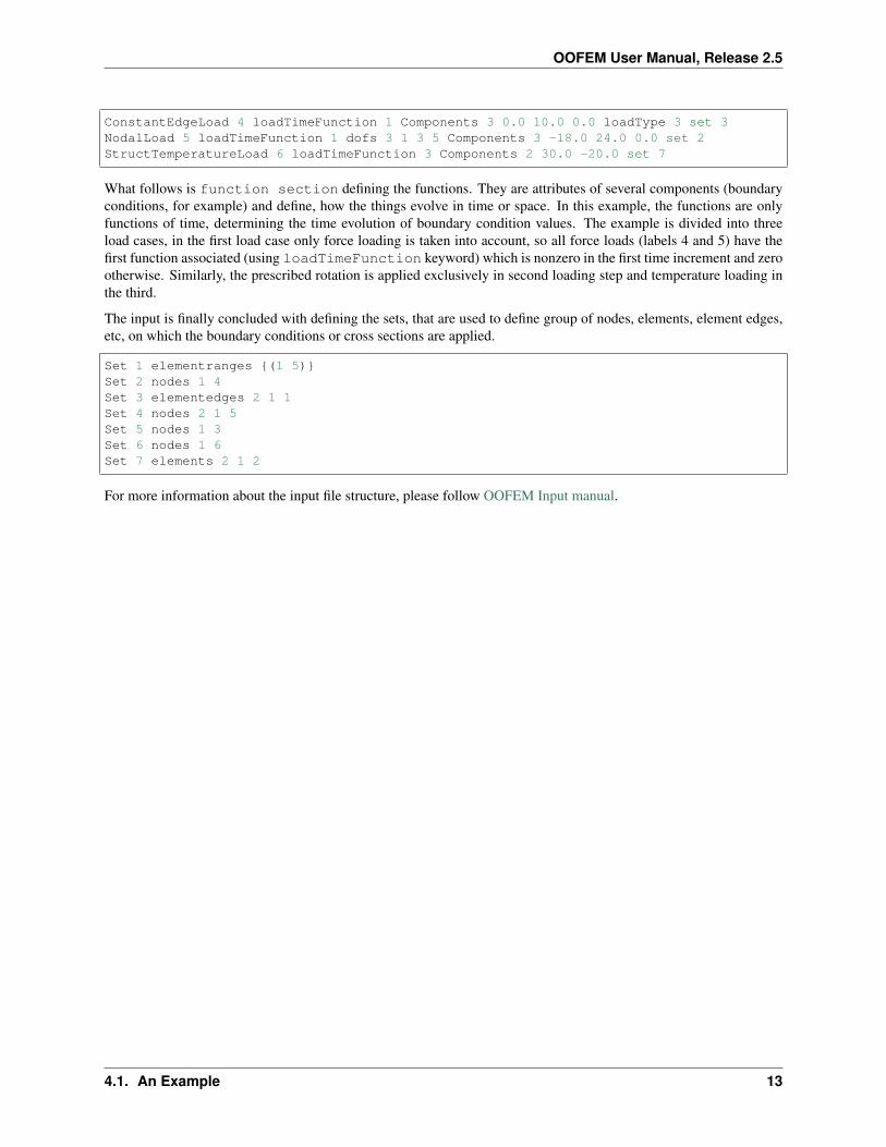
ConstantEdgeLoad 4 loadTimeFunction 1 Components 3 0.0 10.0 0.0 loadType 3 set 3NodalLoad 5 loadTimeFunction 1 dofs 3 1 3 5 Components 3 -18.0 24.0 0.0 set 2StructTemperatureLoad 6 loadTimeFunction 3 Components 2 30.0 -20.0 set 7

What follows is function section defining the functions. They are attributes of several components (boundaryconditions, for example) and define, how the things evolve in time or space. In this example, the functions are onlyfunctions of time, determining the time evolution of boundary condition values. The example is divided into threeload cases, in the first load case only force loading is taken into account, so all force loads (labels 4 and 5) have thefirst function associated (using loadTimeFunction keyword) which is nonzero in the first time increment and zerootherwise. Similarly, the prescribed rotation is applied exclusively in second loading step and temperature loading inthe third.

The input is finally concluded with defining the sets, that are used to define group of nodes, elements, element edges,etc, on which the boundary conditions or cross sections are applied.

Set 1 elementranges {(1 5)}Set 2 nodes 1 4Set 3 elementedges 2 1 1Set 4 nodes 2 1 5Set 5 nodes 1 3Set 6 nodes 1 6Set 7 elements 2 1 2

For more information about the input file structure, please follow OOFEM Input manual.

4.1. An Example 13

OOFEM User Manual, Release 2.5

14 Chapter 4. Understanding input file

CHAPTER

FIVE

UNDERSTANDING OUTPUT FILE

By default, oofem produces output in the form of readable text file, called output file. Its content can be controlled tosome extend in OutputManager record of input file. One can filter output for selected solution steps, and specificsets of nodes and elements, for example.

5.1 An Example

Consider the same linear elastic analysis of beam structure, as in previous section. We first run the solver with theexample

$ ./oofem -f /home/user/oofem.git/tests/sm/beam2d_1.in

Upon the successful execution, the text output file containing simulation results is created (the name of output file isspecified in input file). In our case, the beam2d_1.out file is created in the current working directory. The outputfile can be inspected by any text editor.

5.1.1 Header section

Every output file starts with Header containing information on solver version, job name and starting date and time ofthe analysis

############################################################## www.oofem.org ####### #### ###### ###### # #

# # # # # # ## ### # # # ##### ##### # ## #

# # # # # # # ## # # # # # # # OOFEM ver. 2.6#### #### # ###### # # Copyright (C) 1994-2020 Borek Patzak

################################################################################

Starting analysis on: Wed Jun 9 09:32:17 2021

Homework www sm40 no. 1

15

OOFEM User Manual, Release 2.5

5.1.2 Solution step section(s)

The output file continues with output for each solution step of the analysis. This consists of simple header indicatingthe solution step time

==============================================================Output for time 1.00000000e+00

==============================================================

The output for solution step consists of output of problem domain(s)

Output for domain 1

consisting of output for all nodes and elements. We start with nodal output. The output for each node starts with Nodekeyword, followed by node label and number (in parenthesis). This is followed by indented block containing the outputfor every degree of freedom of the node. DOF meaning is identified by a integer code after dof keyword. The codesare defined by DofIDItem enum. For example, the mechanical unknowns have following codes: 1 for displacementin x direction, 2 for displacement in y direction, 3 for displacement in z direction, 4 for rotation around x axis, 5for rotation around y axis and 6 for rotation around z axis (see src/oofemlib/dofiditem.h for full definition). Our 2Dbeam structure is in xz plane, so the relevant DOFs are displacement in x, displacement in z and rotation around y,corresponding to DOF codes 1,3,5. The d code dof output means that actual value is printed, for some analyses, alsovelocities and accelerations of the corresponding unknown can be printed.

DofManager output:------------------

Node 1 ( 1):dof 1 d -1.37172495e-03dof 3 d 0.00000000e+00dof 5 d -2.38787802e-05

Node 2 ( 2):dof 1 d -1.37172495e-03dof 3 d 2.03123137e-14dof 5 d -1.01549259e-06

Node 3 ( 3):dof 1 d -1.37172495e-03dof 3 d 4.20823351e-05dof 5 d 0.00000000e+00

Node 4 ( 4):dof 1 d -1.75286359e-03dof 3 d 5.50267187e-04dof 5 d 1.05205838e-05

Node 5 ( 5):dof 1 d -1.34016320e-03dof 3 d 0.00000000e+00dof 5 d 4.07440098e-04

Node 6 ( 6):dof 1 d 0.00000000e+00dof 3 d 0.00000000e+00dof 5 d -0.00000000e+00

The nodal output is followed by element output. The actual format depends on particular element, but generallyinternal variables at each integration point are reported. In case of beam element, the local displacements and endforces are printed as well.

Element output:---------------beam element 1 ( 1) :

(continues on next page)

16 Chapter 5. Understanding output file

OOFEM User Manual, Release 2.5

(continued from previous page)

local displacements -1.3717e-03 0.0000e+00 -2.3879e-05 -1.3717e-03 2.0312e-14 -1.→˓0155e-06local end forces 0.0000e+00 -8.9375e+00 0.0000e+00 0.0000e+00 -1.5062e+01 -7.→˓3499e+00GP 1.1 : strains 0.0000e+00 0.0000e+00 0.0000e+00 3.6323e-05 0.0000e+00 0.→˓0000e+00 -2.4500e-33 0.0000e+00

stresses 0.0000e+00 0.0000e+00 0.0000e+00 4.2897e+00 0.0000e+00 0.→˓0000e+00 -3.0625e+00 0.0000e+00GP 1.2 : strains 0.0000e+00 0.0000e+00 0.0000e+00 2.0106e-05 0.0000e+00 0.→˓0000e+00 -2.4500e-33 0.0000e+00

stresses 0.0000e+00 0.0000e+00 0.0000e+00 2.3745e+00 0.0000e+00 0.→˓0000e+00 -3.0625e+00 0.0000e+00GP 1.3 : strains 0.0000e+00 0.0000e+00 0.0000e+00 -1.0531e-06 0.0000e+00 0.→˓0000e+00 -2.4500e-33 0.0000e+00

stresses 0.0000e+00 0.0000e+00 0.0000e+00 -1.2437e-01 0.0000e+00 0.→˓0000e+00 -3.0625e+00 0.0000e+00GP 1.4 : strains 0.0000e+00 0.0000e+00 0.0000e+00 -1.7270e-05 0.0000e+00 0.→˓0000e+00 -2.4500e-33 0.0000e+00

stresses 0.0000e+00 0.0000e+00 0.0000e+00 -2.0396e+00 0.0000e+00 0.→˓0000e+00 -3.0625e+00 0.0000e+00...

For structural analyses the reaction table is reported:

R E A C T I O N S O U T P U T:_______________________________

Node 1 iDof 3 reaction -8.9375e+00 [bc-id: 1]Node 3 iDof 5 reaction 0.0000e+00 [bc-id: 2]Node 5 iDof 3 reaction -1.8750e+01 [bc-id: 1]Node 6 iDof 1 reaction 1.8000e+01 [bc-id: 3]Node 6 iDof 3 reaction -2.0312e+01 [bc-id: 3]Node 6 iDof 5 reaction -5.3999e+01 [bc-id: 3]

Finally, the solution time for every time step is reported.

User time consumed by solution step 1: 0.004 [s]

The output is then repeated for each solution step of the problem. Finally, the accumulated total solution time isreported.

Finishing analysis on: Wed Jun 9 09:32:17 2021

Real time consumed: 000h:00m:00sUser time consumed: 000h:00m:00s

5.1. An Example 17

OOFEM User Manual, Release 2.5

18 Chapter 5. Understanding output file

CHAPTER

SIX

POSTPROCESSING

By default, oofem produces output in the form of readable text file, called output file. At the same time, oofemcan produce output in other formats, that are more suitable for postprocessing in third-party tools. This is done byconfiguring one or more export modules in the input file. In this short tutorial, we will cover vtk postprocessing.

6.1 Configuring vtk export

VTK is a widely used format for storing simulation results. The vtk files can be opened in many visualization tools.The export of results in vtk format can be done using vtkxml export module. The number of export modules isdefined in analysis record using nmodules keyword. The records for export modules should immediately followanalysis record. The detailed syntax of vtkxml record is described in oofem input manual. As an example, consideran example of 3-point bending test input file (located in tests/benchmark/sm/concrete_3point.in) which we modify toadd vtk export:

concrete_3point.outTest: 3-point bending, triangular elements, 1 loaded pointStaticStructural nsteps 4 solverType "calm" stepLength 0.025 rtolf 1e-4 Psi 0.0→˓MaxIter 200 reqIterations 80 HPC 2 1 2 stiffmode 1 nmodules 1vtkxml tstep_all dofman_all element_all primvars 1 1 vars 2 1 4...

The export has been requested for all solution steps tstep_all, all dof managers (nodes) dofman_all andall elements element_all. The primary variables exported consists of displacement vector: primvars 1 1,where primvars is the keyword for primary variable export, what follows is an array of primary variables IDs(defined in src/oofemlib/unknowntype.h), first number determines the array size. The export of secondary (inter-nal) variables consists of strain and stress tensors (vars 2 1 4, where internal variable codes are defined insrc/oofemlib/internalstatetype.h).

After running the modified, extended input the solver will produce for each solution step vtu file.

6.2 Postprocessing in paraview

In this example, we will use Paraview (Open-source, multi-platform data analysis and visualization application,www.paraview.org). After installation of this tool, simply launch paraview and open one or all vtu files produced.

19

OOFEM User Manual, Release 2.5

20 Chapter 6. Postprocessing

CHAPTER

SEVEN

INDICES AND TABLES

• genindex

• modindex

• search

21