Open Archive Toulouse Archive Ouverte (OATAO) OATAO is an open access repository that collects the work of Toulouse researchers and makes it freely available over the web where possible.

This is an author-deposited version published in: http://oatao.univ-toulouse.fr/ Eprints ID: 3286

To link to this article: DOI: 10.1115/1.2910891

URL: http://dx.doi.org/10.1115/1.2910891

To cite this version: MICHON, Guilhem. Parametric instability of an axially moving belt subjected to multifrequency excitations: experiments and analytical validation: 11th Conference on Nonlinear Vibrations, VirginiaTech, USA - 10 December 2009. Journal of Applied Mechanics, 2008, vol. 75, n° 4, pp. 041004.1-041004.8. ISSN 1555-1415

Any correspondence concerning this service should be sent to the repository administrator:staff-oatao@inp-toulouse.fr

1

ersNtlte

badHapm

tavb

awtsb

Guilhem MichonUniversité de Toulouse,

ISAE DMSM,10 Avenue Edouard Belin,

31055 Toulouse, Francee-mail: guilhem.michon@isae.fr

Lionel Manine-mail: lionel.manin@insa-lyon.fr

Didier Remonde-mail: didier.remond@insa-lyon.fr

Regis Dufoure-mail: regis.dufour@insa-lyon.fr

LaMCoS,INSA-Lyon,

CNRS UMR5259,F69621, France

Robert G. ParkerDepartment of Mechanical Engineering,

The Ohio State University,650 Ackerman Road,

Columbus, OH 43202e-mail: parker.242@osu.edu

Parametric Instability of anAxially Moving Belt Subjected toMultifrequency Excitations:Experiments and AnalyticalValidationThis paper experimentally investigates the parametric instability of an industrial axiallymoving belt subjected to multifrequency excitation. Based on the equations of motion, ananalytical perturbation analysis is achieved to identify instabilities. The second partdeals with an experimental setup that subjects a moving belt to multifrequency paramet-ric excitation. A data acquisition technique using optical encoders and based on theangular sampling method is used with success for the first time on a nonsynchronous belttransmission. Transmission error between pulleys, pulley/belt slip, and tension fluctuationare deduced from pulley rotation angle measurements. Experimental results validate thetheoretical analysis. Of particular note is that the instability regions are shifted to lowerfrequencies than the classical ones due to the multifrequency excitation. This experimentalso demonstrates nonuniform belt characteristics (longitudinal stiffness and friction co-efficient) along the belt length that are unexpected sources of excitation. These variationsare shown to be sources of parametric instability. DOI: 10.1115/1.2910891

Keywords: automotive belt, parametric instabilities, multifrequency excitation, experi-mental investigation, angular sampling

IntroductionInstead of classical V belts, serpentine drives are used in front

nd accessory drives FEADs. They use flat and multiribbed beltsunning over multiple accessory pulleys, leading to simplified as-embly and replacement, longer belt life, and compactness 1.umerous mechanical phenomena occur in this application: rota-

ional vibrations 2, hysteretic behavior of belt tensioner 3, non-inear transverse vibration due to the existence of pulley eccen-ricity 4, dry friction tensioner behavior 5, or parametricxcitation.

Commonly known under the category of axially moving media,elt spans are subjected to parametric excitation from their oper-ting environment as studied by Zhang 6. A theoretical nonlinearynamic analysis is also analyzed by Mockenstrum et al. 7,8.owever, only Pellicano et al. 9,10 present a coupled theoretical

nd experimental investigation, where the excitation comes fromulley eccentricity, which causes simultaneous direct and para-etric excitation.Widely used in automotive engines, belt spans experience mul-

ifrequency excitation caused by engine firing and accessory vari-ble torques 11. Belt parametric instability occurs as transverseibration in these applications, where the problems are noise andelt fatigue.

This paper builds on a previous work of Parker and Lin 12 asn experimental illustration and model validation. First, it dealsith the general moving belt model subjected to multifrequency

ension and speed fluctuations. Then a specific test bench is pre-ented, which produce this kind of excitation. Data acquisition isased on the principle of pulse timing method and leads to angular

sampling for frequency analysis 13. This method is applied herefor the first time on a nondiscrete geometry. The theoretical resultsfrom perturbation analysis are compared to the experimental ones.An unexpected source of parametric excitation is also highlighted.

2 Mathematical ModelA mathematical model of an axially moving beam subjected to

multifrequency tension and speed parametric excitation is used toestablish the parametric instability region transition curves. Theequation of motion for transverse vibration of a beam of length Lmoving with time dependent transport velocity cT is governedby 14

AV,TT + c,TV,X + 2cV,TX + c2V,XX − Ps + PdTV,XX + EIV,XXXX

= 0 1

where A is the mass per unit length, EI the bending stiffness, Vthe transverse displacement, Ps the mean belt tension, PdT thedynamic tension, and T and X the independent time and spatialvariables. The dynamic tension results from longitudinal motionof the endpoints as a result of pulley oscillations and quasistaticmidplane stretching from transverse deflection, and is given by

PdT =EA

L UL,T − U0,T +1

20

L

V,X2 dX 2

EA is the longitudinal stiffness modulus and U the longitudinaldisplacement. With the dimensionless parameters,

x,v,u =X,V,U

, t = T Ps , = c Ps

L AL2 A

E

T

wps

rb

w

3

fdtpmi

sb0

=EA

Ps, =

EI

PsL2 , i =AL2

Psi 3

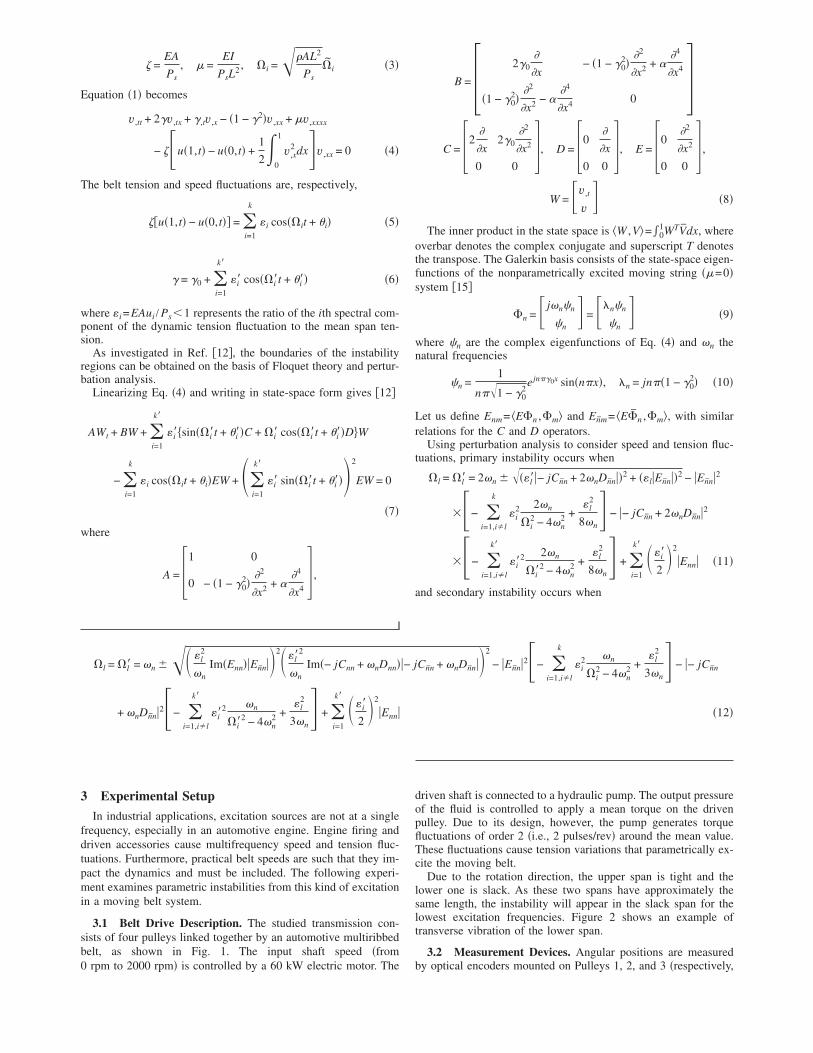
quation 1 becomes

v,tt + 2v,tx + ,tv,x − 1 − 2v,xx + v,xxxx

− u1,t − u0,t +1

20

1

v,x2 dxv,xx = 0 4

he belt tension and speed fluctuations are, respectively,

u1,t − u0,t = i=1

k

i cosit + i 5

= 0 + i=1

k

i cosit + i 6

here i=EAui / Ps1 represents the ratio of the ith spectral com-onent of the dynamic tension fluctuation to the mean span ten-ion.

As investigated in Ref. 12, the boundaries of the instabilityegions can be obtained on the basis of Floquet theory and pertur-ation analysis.

Linearizing Eq. 4 and writing in state-space form gives 12

AWt + BW + i=1

k

isinit + iC + i cosit + iDW

− i=1

k

i cosit + iEW + i=1

k

i sinit + i2

EW = 0

7

here

A = 1 0

0 − 1 − 02

2

2 + 4

4 ,

x x

rpm to 2000 rpm is controlled by a 60 kW electric motor. The

B = 20

x− 1 − 0

22

x2 + 4

x4

1 − 02

2

x2 − 4

x4 0 C = 2

x20

2

x2

0 0, D = 0

x

0 0, E = 0

2

x2

0 0 ,

W = v,t

v 8

The inner product in the state space is W ,V=01WTVdx, where

overbar denotes the complex conjugate and superscript T denotesthe transpose. The Galerkin basis consists of the state-space eigen-functions of the nonparametrically excited moving string =0system 15

n = jnn

n = nn

n 9

where n are the complex eigenfunctions of Eq. 4 and n thenatural frequencies

n =1

n1 − 02ejn0x sinnx, n = jn1 − 0

2 10

Let us define Enm= En ,m and Enm= En ,m, with similarrelations for the C and D operators.

Using perturbation analysis to consider speed and tension fluc-tuations, primary instability occurs when

l = l = 2n l− jCnn + 2nDnn2 + lEnn2 − Enn2

− i=1,il

k

i2 2n

i2 − 4n

2 +l

2

8n − − jCnn + 2nDnn2

− i=1,il

k

i2 2n

i2 − 4n

2 +l

2

8n +

i=1

k i

22

Enn 11

and secondary instability occurs when

l = l = n l2

nImEnnEnn2 l

2

nIm− jCnn + nDnn− jCnn + nDnn2

− Enn2− i=1,il

k

i2 n

i2 − 4n

2 +l

2

3n − − jCnn

+ nDnn2− i=1,il

k

i2 n

i2 − 4n

2 +l

2

3n +

i=1

k i

22

Enn 12

Experimental Setup

In industrial applications, excitation sources are not at a singlerequency, especially in an automotive engine. Engine firing andriven accessories cause multifrequency speed and tension fluc-uations. Furthermore, practical belt speeds are such that they im-act the dynamics and must be included. The following experi-ent examines parametric instabilities from this kind of excitation

n a moving belt system.

3.1 Belt Drive Description. The studied transmission con-ists of four pulleys linked together by an automotive multiribbedelt, as shown in Fig. 1. The input shaft speed from

driven shaft is connected to a hydraulic pump. The output pressureof the fluid is controlled to apply a mean torque on the drivenpulley. Due to its design, however, the pump generates torquefluctuations of order 2 i.e., 2 pulses/rev around the mean value.These fluctuations cause tension variations that parametrically ex-cite the moving belt.

Due to the rotation direction, the upper span is tight and thelower one is slack. As these two spans have approximately thesame length, the instability will appear in the slack span for thelowest excitation frequencies. Figure 2 shows an example oftransverse vibration of the lower span.

3.2 Measurement Devices. Angular positions are measured

by optical encoders mounted on Pulleys 1, 2, and 3 respectively,

2sar

icotb3teatcq

am

048 pulses/rev, 2048 pulses/rev, and 2500 pulses/rev. Belt ten-ion is measured by a piezoelectric sensor on the Pulley 3 supportnd belt lateral vibration by a laser displacement sensor 0.02 mange, 10 m dynamic resolution.

The data acquisition system is custom made with a PXI framencluding classical data acquisition boards and a four-channelounterboard permitting the use of the pulse timing method. Eachptical encoder delivers a square signal TTL as it rotates. Be-ween two rising edges of this signal, a counter records the num-er of pulses given by a high frequency clock 80 MHz, see Fig.. For each encoder, it is therefore possible to build a time vectorhat contains the times of occurence of the TTL signal’s risingdges. Hence, the total rotation angle of each shaft is determinednd instantaneous rotation speed and acceleration are deduced. Inhis application, measurement is triggered on the reference en-oder mounted on the driving shaft and analog signals are ac-uired at each instant of the reference encoder’s rising edge. Ob-

(a)

Fig. 1 Experimental setup for par

Fig. 2 Example of instability in slack belt span

Fig. 3 Angular sampling principle

viously, when an analog signal is sampled in the angular domain,the speed conditions are taken into account in order to set thecutoff frequency of antialiasing filters. An important characteristicof this measurement principle is to separate resolution and preci-sion. Resolution is given by the number of pulses/rev, and thetheoretical angular precision is proportional to the ratio betweenrotation speed and counterclock frequency. The grating quality ofthe optical encoder disk, as well as the electronic signal condition-ing and processing, may also affect the practical accuracy.

3.3 Angular Sampling Benefits. Compared to classical ac-quisition 16, data are resampled based on the angular rotation ofa chosen encoder, which is not necessarily the reference one. Itconsists in calculating the angular rotations of the other encodersat the times corresponding to the rising edges of the samplingencoder. Hence, if angular sampling is performed on encoder i,the angular positions of each of the slave encoders are computedfrom linear interpolation at the times corresponding to the encoderi rising edge locations, see Fig. 4a.

For the analog signals, the same method is applied and they arerecorded at the angular frequency of the reference encoder. Thismethod is called angular sampling and is detailed in Ref. 13. It ismainly applied in rotating machines with synchronous transmis-sion elements, such as gears or timing belts. Its application to atransmission in the presence of belt slip is novel and providesimportant advantages as described below. This technique is espe-cially useful for systems with variable speed because the positionof the sampling points and the angular resolution remain exactlythe same when the speed fluctuates.

As the angular sampling frequency is constant based on theencoder resolution, instead of performing the fast Fourier trans-form FFT analysis in the time domain, this is performed in theangular domain. In other words, the measured signals are treatedas functions of the angular position of the sampling encoder. Thesampling encoder’s position plays the role typically filled by timein classical FFT analysis.

The spectral data are a function of angular frequency, which hasunits of rad−1. The maximum angular frequency is 1 /, where=2 /Ng is the angular resolution of the sampling encoderbased on Ng gratings. Increments on the angular frequency axisare spaced at f =1 /N, where N is the number of samplingencoder rising edges in the collected data. Examples of classicalCampbell and angular frequency diagrams are compared in Fig. 5.On Fig. 5a, natural frequencies are located at a constant fre-quency when speed increases while speed-dependent frequencyorders linearly increase. In the angular frequency domain, how-

b)

etrically excited moving belt drive

(

ever, natural frequencies appear as hyperbola f =1 / and

slt

t

ssl

ms

„a

peed-dependent frequency orders are located at a constant angu-ar frequency f =a · leads to 1 /=a, vertical lines parallel tohe speed axis, see Fig. 5b.

Thus, the main advantages of performing angular sampling inhis application are as follows:

• Sampling points are exactly located in reference to the ge-ometry of the rotating machine, even when speed varies. Itpermits to compare several measurement results based onthe same sampling conditions.

• Spectral analysis is always performed with the same accu-racy and the same resolution. Angular sampling also ensuresthat the magnitude of harmonic components are exactly es-timated 13.

• By choosing Encoder 3 as reference, and assuming that noslip occurs between belt and the idler pulley since no torqueis being transmitted, the sampling points are attached to thebelt.

Therefore, it is more convenient to identify speed-dependent frequency components on a graph with an angu-lar frequency axis related to a chosen reference encoder.

For standard Fourier analysis, it is necessary to get the mea-urements as a function of one single time vector with equallypaced intervals. This requires a time resampling of the data usinginear interpolation, as shown in Fig. 4b.

3.4 Phase Difference Measurement. This angular samplingethod has already been used for many synchronous transmission

tudies gearbox, timing belt drive but never for nonsynchronous

(a)

Fig. 4 Angular resampling method

transmissions, such as serpentine multiribbed belt drives. Thetransmission error is defined as the angular rotation differencebetween shaft i and shaft j,

= i − · j 13

where and i,j are, respectively, the transmission ratio and theangular positions of shaft i, j.

In the case of nonsynchronous belt drive systems, some creepoccurs between the belt and the pulleys due to the power trans-mission by friction 17,18. Indeed, the creep corresponds to therelative slip between the belt and the driven pulley as the beltelongates on the pulley contact arc as its tension increases. Here,the transmission error between Pulleys 3 and 2 is considered.

The rotation of Pulley 3 is not totally transmitted to Pulley 2due to the belt stretching on Pulley 2, which causes a delay.Therefore, the mean value of the transmission error is not zero asit is for a synchronous drive, but rather always increases Fig. 6.In our application, analysis permits decomposition of the observedtransmission error as the sum of a linear function of time repre-senting the transmission error due to the pulley belt creep creep,and the residual transmission error res due to the system dynamicas in synchronous transmission.

= 3 − · 2 = res + creep 14

where creep is identified from as a linear regression of timeassuming a constant mean rotation speed. Removing the linearpart creep from the transmission error yields the zero-mean pe-

b)

… and time resampling method „b…

(

r

bpEaUPptcmpUTat

… t

iodic residual transmission error res Fig. 6.As mentioned in the theoretical model description, the dynamic

elt tension can be expressed as the difference of the endpointositions and midplane stretching from transverse vibration, seeq. 2. Considering the belt span that connects Pulleys 3 and 2,nd taking into account the belt translation direction, UL ,T and0,T correspond, respectively, to the belt unseating point onulley 3 and to the belt seating point on Pulley 2. These twooints are not fixed in space since pulley rotations oscillate aroundhe linearly increasing angles w3t and w2t. Assuming a no-slipondition at these two points, UL ,T and U0,T can be esti-ated from pulley angle oscillations multiplied by the respective

ulley pitch radius. Finally, the difference between UL ,T and0,T corresponds to the residual transmission error at time T.herefore, residual transmission error and belt tension fluctuationre related. Figure 7 presents the measured progression of beltension and residual transmission error angular waterfall analysis

0 0.1 0.2 0.3 0.4 0.5 0.60

0.5

1

1.5

2

2.5

3

3.5

4

Time (s)

Tra

nsm

issi

oner

ror

(a)

Fig. 6 Total „a… and residual „b

Fig. 7 Belt tension and transmissio

function of rotation speed

with change in rotation speed note that all waterfall plots are topviews. The same frequency components appear on each graphand prove that the measurement system with optical encoders andangular sampling permits evaluation of belt tension fluctuation.Finally, this analysis shows that the transmission error includesthe pulley belt creep plus the system dynamic.

3.5 Nonuniform Belt Characteristic Identification andConsequences. The low modulation observed on the dynamictransmission error Fig. 6 corresponds to the belt traveling fre-quency and demonstrates that there are nonuniform belt charac-teristics. In order to check this nonuniformity, a belt has been cutin ten equal parts. Each part has been tested to determine longi-tudinal rigidity modulus k and damping C. Each belt sample isclamped at one end and has a mass m suspended at the other, seeFig. 8. This system is excited via a shock hammer. The free re-sponse is recorded via an accelerometer and postprocessed to ob-

0 0.1 0.2 0.3 0.4 0.5 0.6−0.03

−0.02

−0.01

0

0.01

0.02

0.03

Time (s)

Res

idua

ltra

nsm

issi

oner

ror

b)

ransmission error versus time

rror angular top-view waterfall as a

(

n e

Fidentification

FCi max

fluctuation

tain belt longitudinal stiffness and damping. Longitudinal damp-ing coefficients of belt samples, normed by the maximummeasured value, are plotted versus belt sample number in Fig. 9.Non-negligible variation is observed for C while local stiffness,and therefore EA, is constant. This irregularity is probably due tothe manufacturing process printing, cord winding, cutting. Thelow frequency modulation observed is shown to be a parametricexcitation source next.

4 Belt Span Instability Analysis

4.1 Experimental Investigation. On the global experimentalsetup for a given initial belt tension and mean torque, a speedsweep of the driving shaft is performed from 532 rpmto 1512 rpm in 14 rpm increments 70 tests. The experimentalresults are presented in Fig. 10 as a top-view waterfall in theangular frequency domain for a the transverse vibration, b belttension, and c belt speed. All parameters are dimensionless asdefined in Sec. 2 waterfall FFT in the time-frequency domain aregiven in Appendix.

The belt tension angular waterfall, Fig. 10b, exhibits linesparallel to the speed axis, which proves a speed-dependent exci-tation. The belt transverse vibration angular waterfall is presentedon Fig. 10a. The instabilities are represented by the black spotslocated on a hyperbola. which proves parametric instability. Thesystem is unstable for numerous frequencies.

4.2 Main Instability Regions. The main excitation of thesystem comes from the pump design, which creates torque fluc-tuations of order 2, inducing speed and tension fluctuations. Re-garding belt instability, speed variation is a negligible source ofexcitation compared to the tension fluctuation. The latter is ob-served to be the principle source of parametric excitation and islocated on the angular frequency waterfall graph at abscissa 2.60as a vertical line. Primary and secondary instability regions,circled on Fig. 10a, are the response to this torque excitation.

Experimentally, the primary instability occurs for 1 7.9,8.8. This region is classically wider than the correspond-ing secondary region which occurs for 1 4.1,4.5, but alsoshifted of 0.3 from 21 toward lower frequencies due to the mul-tifrequency excitation.

Considering the small transverse rigidity modulus and the largespan length in this application, the bending stiffness modulus isneglected. Therefore, in the following, the belt span is consideredas a string =0. Thus, using Eqs. 7 and 8 and Cnn= 1−e−2jn0 /2, Dnn=0, Enn= 1−e−2jn0 / 40, and Enn= jn1+0

2 /2. The experimental parameters introduced in the model are0=0.5, 1=4.3, 2=8, 2=8, 1=0.001, 2=0.3, 2=0.001. For1=0.7, the instability region occurs for 1 7.8 9.2.

(c)

rse vibration, „b… belt tension fluctuation, „c… belt speed

(a) (b)

ig. 8 Experimental setup for the local belt characteristics

1 2 3 4 5 6 7 8 9 100.75

0.8

0.85

0.9

0.95

1

Belt sample number

Rel

ativ

eda

mpi

ng

ig. 9 Dimensionless damping evolution along the belt length/C

(a) (b)

Fig. 10 Experimental angular top-view waterfall: „a… transve

esco

mbpsir

5

dt

F„

The instability region boundaries are plotted as a function of thexcitation amplitude 1 in Fig. 11. When 221, the secondource of excitation shift the instability region to lower frequen-ies. While this phenomenon is not classical, the experimentalbservations confirm the theoretical results of Ref. 12.

4.3 Low Amplitude Instability Region. The low frequencyodulation observed on the residual transmission error due to the

elt characteristic irregularity highlighted in Sec. 3.5 is a source ofarametric excitation. It appears on the waterfall plot of the ten-ion fluctuation as low level parallel lines separated by 0.20, thats, the belt traveling frequency. This irregularity explains the pe-ipheral instabilities presented on Fig. 10a.

ConclusionThis paper focuses on an experimental investigation of an in-

ustrial axially moving belt subjected to multifrequency excita-

3 4 5 6 7 8 9 100

0.1

0.2

0.3

0.4

0.5

0.6

0.7

0.8

0.9

1

Ω1

ε 1

ω1 2ω

1

ig. 11 Instability region. Model „solid line… and experimentstars….

0 1 2 3 4 5 6 7 8

x 104

3

4

5

6

7

8

Frequency

Om

eg

a

0 1 2 3

3

4

5

6

7

8

Om

eg

a

(a) (

Fig. 12 Experimental classical Campbell-like diagram top-viebelt speed fluctuation „c…

ion. Comparison with analytical results from a perturbation

analysis is presented and permits to validate theoretical instabili-ties. The main conclusion are as follows:

• Parametric instabilities occur in experimental system suchas belt drive.

• Measurement system based on angular sampling is shown tobe an efficient tool for instability analysis in belt drive sys-tems.

• Irregular belt characteristics have been detected and high-lighted as unexpected source of parametric excitation.

• Instability regions are shifted when subjected to multifre-quency excitation.

• Experimental observations confirm the theoretical results.

Further analysis will focus on the role of the hysteretic behaviorof the belt tensioners on these instabilities.

AppendixFigure 12 represents the top-view waterfall in the classical

Campbell-like diagram.

References1 Gerbert, G., 1981, “Some Notes on V-Belt Drives,” ASME J. Mech. Des.,

103, pp. 8–18.2 Hwang, S. J., Perkins, N. C., Ulsoy, A., and Meckstroth, R. J., 1994, “Rota-

tional Response and Slip Prediction of Serpentine Belt Dirve Systems,” ASMEJ. Vibr. Acoust., 116, pp. 71–78.

3 Michon, G., Manin, L., and Dufour, R., 2005, “Hysteretic Behavior of a BeltTensioner, Modeling and Experimental Investigation,” J. Vib. Control, 119,pp. 1147–1158.

4 Wickert, J. A., 1992, “Non-Linear Vibration of a Traveling Tensioned Beam,”Int. J. Non-Linear Mech., 273, pp. 503–517.

5 Leamy, M. J., and Perkins, N. C., 1998, “Nonlinear Periodic Response ofEngine Accessory Drives With Dry Friction Tensioners,” ASME J. Vibr.Acoust., 120, pp. 909–916.

6 Zhang, L., and Zu, J. W., 1999, “One-to-One Auto-Parametric Resonance inSerpentine Belt Drive Systems,” J. Sound Vib., 232, pp. 783–806.

7 Mockensturm, E., Perkins, N., and Ulsoy, A., 1996, “Stability and LimitCycles of Parametrically Excited, Axially Moving Strings,” ASME J. Vibr.Acoust., 118, pp. 346–351.

8 Mockensturm, E. and Guo, J., 2005, “Nonlinear Vibration of ParametricallyExcited Viscoelastic Axially Moving Media,” ASME J. Appl. Mech., 72, pp.374–380.

9 Pellicano, F., Catellani, G., and Fregolent, A., 2004, “Parametric Instability of

5 6 7 8

x 104ncy

0 1 2 3 4 5 6 7 8

x 104

3

4

5

6

7

8

Frequency

Om

eg

a

(c)

aterfall: transverse vibration „a…, belt tension fluctuation „b…,

4Freque

b)

w w

Belts, Theory and Experiments,” Comput. Struct., 82, pp. 81–91.

10 Pellicano, F., Fregolent, A., Bertuzzi, A., and Vestroni, F., 2001, “Primary andParametric Non-Linear Resonances of a Power Transmission Belt: Experimen-tal and Theoretical Analysis,” J. Sound Vib., 244, pp. 669–684.

11 Cheng, G., and Zu, J. W., 2003, “Nonstick and Stick-Slip Motion of aCoulomb-Damped Belt Drive System Subjected to Multifrequency Excita-tions,” ASME J. Appl. Mech., 70, pp. 871–884.

12 Parker, R., and Lin, Y., 2001, “Parametric Instability of Axially Moving MediaSubjected to Multifrequency Tension and Speed Fluctuation,” ASME J. Appl.Mech., 68, pp. 49–57.

13 Remond, D., and Mahfoudh, J., 2005, “From Transmission Error Measure-ments to Angular Sampling in Rotating Machines With Discrete Geometry,”Shock Vib., 9, pp. 1–13.

14 Thurman, A. L., and Mote, C. D., Jr., 1969, “Free, Periodic, Non-Linear Os-cillation of an Axially Moving String,” ASME J. Appl. Mech., 36, pp. 83–91.

15 Jha, R., and Parker, R., 2000, “Spatial Discretization of Axially Moving MediaVibration Problems,” ASME J. Vibr. Acoust., 122, pp. 290–294.

16 Houser, D. R., and Blankenshio, G. W., 1989, “Methods for Measuring Trans-mission Error Under Load and at Operating Speeds,” SAE Trans., 986, pp.1367–1374.

17 Gerbert, G., and Sorge, F., 2002, “Full Sliding Adhesive-Like Contact ofV-Belts,” ASME J. Mech. Des., 124, pp. 706–712.

18 Betchel, S. E., Vohra, S., Jacob, K. I., and Carslon, C. D., 2000, “The Stretch-ing and Slipping of Belts and Fibers on Pulleys,” ASME J. Appl. Mech., 67,pp. 197–206.