Open Quantum Assembly Language

Andrew W. Cross, Lev S. Bishop, John A. Smolin, Jay M. Gambetta

January 10th, 2017

1 Background

Software architectures, compilers, and languages specifically for quantum computing havebeen studied by the academic community for more than a decade ([1–4] and referencestherein). Researchers have implemented software and simulators that can be used in practiceto study quantum algorithms at many scales. While we cannot survey this work here, welist a few of these projects, several of which include software that has been made readilyavailable: Liquid [5, 6], Scaffold [7, 8], Quipper [9–11], ProjectQ [12, 13], QCL [14, 15],Quiddpro [16, 17], Chisel-q [18, 19], and Quil [20, 21].

Our goal in this document is to describe an interface language for the Quantum Expe-rience that enables experiments with small depth quantum circuits. The language can begenerated by the Composer, hand-written, or targeted by higher level software tools, suchas those above. Before we do so, we discuss quantum programs in general to provide con-text. General quantum programs require coordination of quantum and classical parts ofthe computation. One way to think about general quantum programs is to identify theirdistinct phases of execution [11]. Fig. 1 shows a high-level diagram of the processes andabstractions involved in specifying a quantum algorithm, transforming the algorithm intoexecutable form, running an experiment or simulation, and analyzing the results. A key ideathroughout these processes is the use of intermediate representations. An intermediate rep-resentation (IR) of a computation is neither its source language description, nor the targetmachine instructions, but something in between. Compilers may use several IRs during theprocess of translating and optimizing a program.

Compilation. This phase takes place on a classical computer in a setting where specificproblem parameters are not yet known and no interaction with the quantum computer isrequired, i.e. it is offline. The input is source code describing a quantum algorithm and anycompile time parameters. The output is a combined quantum/classical program expressedusing a high level IR. During this phase, it is possible to compile classical procedures intoobject code and make initial passes that do not require complete knowledge of the problemparameters.

Circuit generation. This takes place on a classical computer in an environment wherespecific problem parameters are now known, and some interaction with the quantum com-puter may occur, i.e. this is an online phase. The input is a quantum/classical programexpressed using a high level IR, as well as all remaining problem parameters. The output

1

arX

iv:1

707.

0342

9v2

[qu

ant-

ph]

13

Jul 2

017

is a collection of quantum circuits, or quantum basic blocks, together with associated clas-sical control instructions and classical object code needed at run-time. A basic block is astraight-line code sequence with no branches (except at the entry and exit points). Sincefeedback can occur on multiple time scales, the quantum circuits may include instructionsfor fast feedback. Other classical control instructions outside of the quantum circuit basicblock include, for example, run-time parameter computations and measurement-dependentbranches. External classical object code could include algorithms to process measurementoutcomes into control flow conditions or results, or to generate new basic blocks on the fly.The output of circuit generation is expressed using a quantum circuit IR. Further circuitgeneration may occur based on processed measurement results.

Execution. This takes place on physical quantum computer controllers in a real-timeenvironment, i.e. the quantum computer is active. The input is a collection of quantumcircuits and associated run-time control statements expressed using a quantum circuit IR.The input is processed by a high-level controller into a stream of real-time instructionsin a low-level format that corresponds to physical operations. These are executed on alow-level controller, and a corresponding results stream provides measurement data backto the high-level controller when needed. In general, the high level controller (or virtualmachine) can execute classical control instructions and external object code. The output ofcircuit execution is a collection of processed measurement results returned from the high-levelcontroller.

Post-processing. This takes place on a classical computer after all real-time processingis complete. The input is a collection of processed measurement results, and the outputis intermediate results for further circuit generation and/or the final result of the quantumcomputation.

Quantumalgorithm

Quantumcircuit(s)

(+ classical control)

SystemcontrolRstream

Systemindependent

transformations

Systemdependent

transformations

HighRlevelcompilationRand

optimization

SimulationR/ExperimentR

ControllerR:low2

Requestedresults

Analysis

SimulationR/ExperimentR

ControllerR:high2

scheduleRandRissue

:real4time2

useRspecificRproblemRparameters

QuantumPRclassicalprogram

parallelRexecution:real4time2

PhaseR1:RcompileRtime PhaseR2:RcircuitRgeneration PhaseR3:RcircuitRexecution

RawRsystemresultRstream

SystemRstate

Algorithmoutput

:offline2

APIRPResourceManager

:online2

PhaseR4:Rpost4processing

:online2

:online2

passRto/fromselectedRbackends

Processedresults

Validatedquantumcircuit(s)

(+ classical control)

Analysis

:offline2

interactRwithRbackends

circuit generation

Figure 1: Block diagrams of processes (blue) and abstractions (red) to transform andexecute a quantum algorithm. The emphasized quantum circuit abstraction is the mainfocus of this document. The API and Resource Manager (green) represents the gateway tobackend processes for circuit execution. Dashed vertical lines separate offline, online, andreal-time processes.

2

Our model of program execution on the Quantum Experience does not allow fully generalclassical computations in the loop with quantum computations, as described above, becausequbits remain coherent for a limited time. Quantum programs are broken into distinctcircuits whose quantum outputs cannot be carried over into the next circuit. Classicalcomputation is done between quantum circuit executions. Users actively participate in thecircuit generation phase and manually implement part of feedback path through the highlevel controller in Fig. 1, observing outcomes from the previous quantum circuit and choosingthe next quantum circuit to execute. Making use of an API to the execution phase, userscan write their own software for compilation and circuit generation that interacts with thehardware over a sequence of quantum circuit executions. After obtaining all of the processedresults, users may post-process the data offline.

We specify part of a quantum circuit intermediate representation based on the quantumcircuit model, a standard formalism for quantum computation [22]. The quantum circuitabstraction is emphasized in Fig. 1. The IR expresses quantum circuits with fast feedback,such as might constitute the basic blocks of a full-featured IR. A basic block is a straight-linecode sequence with no branches (except at the entry and exit points). We have chosen toinclude statements that are essential for near-term experiments and that we believe will bepresent in any future IR. The representation will be quite familiar to experts.

The human-readable form of our quantum circuit IR is based on “quantum assemblylanguage” [3, 23–26] or QASM (pronounced kazm). QASM is a simple text language thatdescribes generic quantum circuits. QASM can represent a completely unrolled quantumprogram whose parameters have all been specified. Most QASM variants assume a discreteset of quantum gates, but our IR is designed to control a physical system with a parameterizedgate set. While we use the term “quantum assembly language”, this is merely an analogyand should not be taken too far.

Open QASM represents universal physical circuits, so we propose a built-in gate basisof arbitrary single-qubit gates and a two-qubit entangling gate (CNOT) [27]. We choose asimple language without higher level programming primitives. We define different gate setsusing a subroutine-like mechanism that hierarchically specifies new unitary gates in terms ofbuilt-in gates and previously defined gate subroutines. In this way, the built-in basis is used todefine hardware-supported operations via standard header files. The subroutine mechanismallows limited code reuse by hierarchically defining more complex operations [7, 26]. We alsoadd instructions that model a quantum-classical interface, specifically measurement, statereset, and the most elemental classical feedback.

The remaining sections of this document specify Open QASM and provide examples.

2 Language

The syntax of the human-readable form of Open QASM has elements of C and assemblylanguages. The first (non-comment) line of an Open QASM program must be OPENQASM

M.m; indicating a major version M and minor version m. Version 2.0 is described in thisdocument. The version keyword cannot occur multiple times in a file. Statements areseparated by semicolons. Whitespace is ignored. The language is case sensitive. Commentsbegin with a pair of forward slashes and end with a new line. The statement include

3

q[0]q[1]r[0]r[1]

CX q[0],r[0];

q[0]q[1]r[0]r[1]

CX q,r;

q[0]q[1]r[0]r[1]

CX q,r[0];

q[0]q[1]r[0]r[1]

CX q[0],r;

Figure 2: The built-in two-qubit entangling gate is the controlled-NOT gate. If a andb are qubits, the statement CX a,b; applies a controlled-NOT (CNOT) gate that flipsthe target qubit b iff the control qubit a is one. If a and b are quantum registers, thestatement applies CNOT gates between corresponding qubits of each register. There is asimilar meaning when a is a qubit and b is a quantum register and vice versa.

q[0]

U(θ,φ,λ) q[0];

U(θ,φ,λ)q[0]q[1]

U(θ,φ,λ) q;

U(θ,φ,λ)

U(θ,φ,λ)

Figure 3: The single-qubit unitary gates are built in. These gates are parameterized bythree real parameters θ, φ, and λ. If the argument q is a quantum register, the statementapplies size(q) gates in parallel to the qubits of the register.

"filename"; continues parsing filename as if the contents of the file were pasted at thelocation of the include statement. The path is specified relative to the current workingdirectory.

The only storage types of Open QASM (version 2.0) are classical and quantum registers,which are one-dimensional arrays of bits and qubits, respectively. The statement qreg

name[size]; declares an array of qubits (quantum register) with the given name and size.Identifiers, such as name, must start with a lowercase letter and can contain alpha-numericcharacters and underscores. The label name[j] refers to a qubit of this register, wherej ∈ {0, 1, . . . , size(name)−1}. The qubits are initialized to |0〉. Likewise, creg name[size];

declares an array of bits (register) with the given name and size. The label name[j] refersto a bit of this register, where j ∈ {0, 1, . . . , size(name)− 1}. The bits are initialized to 0.

The built-in universal gate basis is “CNOT + U(2)”. There is one built-in two-qubitgate (Fig. 2)

CNOT :=

1 0 0 00 1 0 00 0 0 10 0 1 0

(1)

called the controlled-NOT gate. The statement CX a,b; applies a CNOT gate that flipsthe target qubit b if and only if the control qubit a is one. The arguments cannot refer tothe same qubit. Built-in gates have reserved uppercase keywords. If a and b are quantumregisters with the same size, the statement means apply CX a[j], b[j]; for each index j

4

into register a. If instead, a is a qubit and b is a quantum register, the statement meansapply CX a, b[j]; for each index j into register b. Finally, if a is a quantum register andb is a qubit, the statement means apply CX a[j], b; for each index j into register a.

All of the single-qubit unitary gates are also built in (Fig. 3) and parameterized as

U(θ, φ, λ) := Rz(φ)Ry(θ)Rz(λ) =

(e−i(φ+λ)/2 cos(θ/2) −e−i(φ−λ)/2 sin(θ/2)ei(φ−λ)/2 sin(θ/2) ei(φ+λ)/2 cos(θ/2)

). (2)

Here Ry(θ) = exp(−iθY/2) and Rz(φ) = exp(−iθZ/2). This specifies any element ofSU(2). When a is a quantum register, the statement U(theta,phi,lambda) a; meansapply U(theta,phi,lambda) a[j]; for each index j into register a. The real parametersθ ∈ [0, 4π), φ ∈ [0, 4π), and λ ∈ [0, 4π) are given by parameter expressions constructedusing in-fix notation. These support scientific calculator features with arbitrary precisionreal numbers1. For example, U(pi/2,0,pi) q[0]; applies a Hadamard gate to qubit q[0].Open QASM (version 2.0) does not provide a mechanism for computing parameters basedon measurement outcomes.

New gates can be defined as unitary subroutines using the built-in gates, as shown inFig. 4. These can be viewed as macros whose expansion we defer until run-time. Gates aredefined by statements of the form

// comment

gate name(params) qargs

{

body

}

where the optional parameter list params is a comma-separated list of variable parameternames, and the argument list qargs is a comma-separated list of qubit arguments. Both theparameter names and qubit arguments are identifiers. If there are no variable parameters,the parentheses are optional. At least one qubit argument is required. The first commentmay contain documentation, such as TeX markup, to be associated with the gate. Thearguments in qargs cannot be indexed within the body of the gate definition.

// this is ok:

gate g a

{

U(0,0,0) a;

}

// this is invalid:

gate g a

{

U(0,0,0) a[0];

}

1 Features include scientific notation; real arithmetic; logarithmic, trigonometic, and exponential functions;square roots; and the built-in constant π. The Quantum Experience uses a double precision floating pointtype for real numbers.

5

q[0]q[1]

cu1(π2

)=

U(0,0,π4)

U(0,0,−π4) U(0,0,π

4)

gate cu1(lambda) a,b

{

U(0,0,theta/2) a;

CX a,b;

U(0,0,-theta/2) b;

CX a,b;

U(0,0,theta/2) b;

}

cu1(pi/2) q[0],q[1];

Figure 4: New gates are defined as unitary subroutines. The gates are applied usingthe statement name(params) qargs; just like the built-in gates. The parentheses areoptional if there are no parameters. The gate cu1(θ) corresponds to the unitary matrixdiag(1, 1, 1, eiθ) up to a global phase.

Only built-in gate statements, calls to previously defined gates, and barrier statements canappear in body. The statements in the body can only refer to the symbols given in theparameter or argument list, and these symbols are scoped only to the subroutine body.An empty body corresponds to the identity gate. Subroutines must be declared before useand cannot call themselves. The statement name(params) qargs; applies the subroutine,and the variable parameters params are given as parameter expressions. The gate can beapplied to any combination of qubits and quantum registers of the same size as shown inthe following example. The quantum circuit given by

gate g qb0,qb1,qb2,qb3

{

// body

}

qreg qr0[1];

qreg qr1[2];

qreg qr2[3];

qreg qr3[2];

g qr0[0],qr1,qr2[0],qr3; // ok

g qr0[0],qr2,qr1[0],qr3; // error!

has a second-to-last line that means

for j ← 0, 1 dog qr0[0],qr1[j],qr2[0],qr3[j];

We provide this so that user-defined gates can be applied in parallel like the built-in gates.To support gates whose physical implementation may be possible, but whose definition

is unspecified, we provide an “opaque” gate declaration. This may be used in practice inseveral instances. For example, the system may evolve under some fixed but uncharacterized

6

q[0]c[0]

q[0] c[0]q[0]c 2 0

q[0]c[0]

2

2

2

2

q[0]q[1]c[0]c[1]

q[0]q[1]c 2 0 1

Figure 5: The measure statement projectively measures a qubit or each qubit of a quan-tum register. The measurement projects onto the Z-basis and leaves qubits available forfurther operations. The top row of circuits depicts single-qubit measurement using thestatement measure q[0] -> c[0]; while the bottom depicts measurement of an entireregister using the statement measure q -> c;. The center circuit of the top row depictsmeasurement as the final operation on q[0].

q[0]

reset q[0];

|0〉q[0]q[1]

reset q;

|0〉

|0〉q

reset q;

2 |0〉 2

Figure 6: The reset statement prepares a qubit or quantum register in the state |0〉.

drift Hamiltonian for some fixed amount of time. The system might be subject to an n-qubitoperator whose parameters are computationally challenging to estimate. The syntax for anopaque gate declaration is the same as a gate declaration but without a body.

Measurement is shown in Fig. 5. The statement measure qubit|qreg -> bit|creg;

measures the qubit(s) in the Z-basis and records the measurement outcome(s) by overwritingthe bit(s). Measurement corresponds to a projection onto one of the eigenstates of Z, andqubit(s) are immediately available for further quantum computation. Both arguments mustbe register-type, or both must be bit-type. If both arguments are register-type and have thesame size, the statement measure a -> b; means apply measure a[j] -> b[j]; for eachindex j into register a.

The reset qubit|qreg; statement resets a qubit or quantum register to the state |0〉.This corresponds to a partial trace over those qubits (i.e. discarding them) before replacingthem with |0〉〈0|, as shown in Fig. 6.

There is one type of classically-controlled quantum operation: the if statement shownin Fig. 7. The if statement conditionally executes a quantum operation based on the valueof a classical register. This allows measurement outcomes to determine future quantumoperations. We choose to have one decision register for simplicity. This register is interpretedas an integer, using the bit at index zero as the low order bit. The quantum operationexecutes only if the register has the given integer value. Only quantum operations, i.e. built-in gates, gate (and opaque) subroutines, preparation, and measurement, can be prefacedby if. A quantum program with a parameter that depends on values that are known only

7

q[0]c

==3

2

U(θ,φ,λ)q[0]c[0]c[1]

==3

U(θ,φ,λ)

Figure 7: The if statement applies a quantum operation only if a classical reg-ister has the indicated integer value. These circuits depict the statement if(c==3)

U(theta,phi,lambda) q[0];.

at run-time can be rewritten using a sequence of if statements. Specifically, for a single-parameter gate with n bits of precision, we may choose to write 2n statements, only oneof which is executed, or we can decompose the parameterized gate into a sequence of nconditional gates.

The barrier instruction prevents optimizations from reordering gates across its sourceline. For example,

CX r[0],r[1];

h q[0];

h s[0];

barrier r,q[0];

h s[0];

CX r[1],r[0];

CX r[0],r[1];

will prevent an attempt to combine the CNOT gates but will allow the pair of h s[0]; gatesto cancel.

Open QASM statements are summarized in Table 1. The grammar is presented in Ap-pendix A.

8

Table 1: Open QASM language statements (version 2.0)

Statement Description Example

OPENQASM 2.0; Denotes a file in Open QASM formata OPENQASM 2.0;

qreg name[size]; Declare a named register of qubits qreg q[5];

creg name[size]; Declare a named register of bits creg c[5];

include "filename"; Open and parse another source file include "qelib1.inc";

gate name(params) qargs { body } Declare a unitary gate (see text)opaque name(params) qargs; Declare an opaque gate (see text)// comment text Comment a line of text // oops!

U(theta,phi,lambda) qubit|qreg; Apply built-in single qubit gate(s)b U(pi/2,2*pi/3,0) q[0];

CX qubit|qreg,qubit|qreg; Apply built-in CNOT gate(s) CX q[0],q[1];

measure qubit|qreg -> bit|creg; Make measurement(s) in Z basis measure q -> c;

reset qubit|qreg; Prepare qubit(s) in |0〉 reset q[0];

gatename(params) qargs; Apply a user-defined unitary gate crz(pi/2) q[1],q[0];

if(creg==int) qop; Conditionally apply quantum operation if(c==5) CX q[0],q[1];

barrier qargs; Prevent transformations across this source line barrier q[0],q[1];

a This must appear as the first non-comment line of the file.b The parameters theta, phi, and lambda are given by parameter expressions; see text and Appendix A.

9

3 Examples

This section gives several examples of quantum circuits expressed in Open QASM (version2.0). The circuits use a gate basis defined for the Quantum Experience.

3.1 Quantum Experience standard header

The Quantum Experience standard header defines the gates that are implemented by thehardware, gates that appear in the Quantum Experience composer, and a hierarchy of ad-ditional user-defined gates. Our approach is to define physical gates that the hardwareimplements in terms of the abstract gates U and CX. The current physical gates supportedby the Quantum Experience are a superset of the abstract gates, but this is not true ofall physical gate sets and devices. Choosing to use abstract gates merely to define physicalgates gives some flexibility to add or change physical gates at a later time without changingOpen QASM. We believe this approach is preferable to invisibly compiling abstract gates tophysical gates or to changing the underlying set of abstract gates whenever the hardwarechanges.

The Quantum Experience currently implements the controlled-NOT gate via the cross-resonance interaction and implements three distinct types of single-qubit gates. The one-parameter gate

u1(λ) := diag(1, eiλ) ∼ U(0, 0, λ) = Rz(λ) (3)

changes the phase of a carrier without applying any pulses. The symbol “∼” denotes equiv-alence up to a global phase. The gate

u2(φ, λ) := U(π/2, φ, λ) = Rz(φ+π

2)Rx(π/2)Rz(λ−

π

2) (4)

uses a single π/2-pulse. The most general single-qubit gate

u3(θ, φ, λ) := U(θ, φ, λ) = Rz(φ+ 3π)Rx(π/2)Rz(θ + π)Rx(π/2)Rz(λ) (5)

uses a pair of π/2-pulses.

// Quantum Experience (QE) Standard Header

// file: qelib1.inc

// --- QE Hardware primitives ---

// 3-parameter 2-pulse single qubit gate

gate u3(theta,phi,lambda) q { U(theta,phi,lambda) q; }

// 2-parameter 1-pulse single qubit gate

gate u2(phi,lambda) q { U(pi/2,phi,lambda) q; }

// 1-parameter 0-pulse single qubit gate

gate u1(lambda) q { U(0,0,lambda) q; }

// controlled-NOT

10

gate cx c,t { CX c,t; }

// idle gate (identity)

gate id a { U(0,0,0) a; }

// --- QE Standard Gates ---

// Pauli gate: bit-flip

gate x a { u3(pi,0,pi) a; }

// Pauli gate: bit and phase flip

gate y a { u3(pi,pi/2,pi/2) a; }

// Pauli gate: phase flip

gate z a { u1(pi) a; }

// Clifford gate: Hadamard

gate h a { u2(0,pi) a; }

// Clifford gate: sqrt(Z) phase gate

gate s a { u1(pi/2) a; }

// Clifford gate: conjugate of sqrt(Z)

gate sdg a { u1(-pi/2) a; }

// C3 gate: sqrt(S) phase gate

gate t a { u1(pi/4) a; }

// C3 gate: conjugate of sqrt(S)

gate tdg a { u1(-pi/4) a; }

// --- Standard rotations ---

// Rotation around X-axis

gate rx(theta) a { u3(theta,-pi/2,pi/2) a; }

// rotation around Y-axis

gate ry(theta) a { u3(theta,0,0) a; }

// rotation around Z axis

gate rz(phi) a { u1(phi) a; }

// --- QE Standard User-Defined Gates ---

// controlled-Phase

gate cz a,b { h b; cx a,b; h b; }

// controlled-Y

gate cy a,b { sdg b; cx a,b; s b; }

// controlled-H

gate ch a,b {

h b; sdg b;

cx a,b;

h b; t b;

cx a,b;

t b; h b; s b; x b; s a;

}

11

// C3 gate: Toffoli

gate ccx a,b,c

{

h c;

cx b,c; tdg c;

cx a,c; t c;

cx b,c; tdg c;

cx a,c; t b; t c; h c;

cx a,b; t a; tdg b;

cx a,b;

}

// controlled rz rotation

gate crz(lambda) a,b

{

u1(lambda/2) b;

cx a,b;

u1(-lambda/2) b;

cx a,b;

}

// controlled phase rotation

gate cu1(lambda) a,b

{

u1(lambda/2) a;

cx a,b;

u1(-lambda/2) b;

cx a,b;

u1(lambda/2) b;

}

// controlled-U

gate cu3(theta,phi,lambda) c, t

{

// implements controlled-U(theta,phi,lambda) with target t and control c

u1((lambda-phi)/2) t;

cx c,t;

u3(-theta/2,0,-(phi+lambda)/2) t;

cx c,t;

u3(theta/2,phi,0) t;

}

3.2 Quantum teleportation

Quantum teleportation (Fig. 8) demonstrates conditional application of future gates basedon prior measurement outcomes.

12

q[0] |0〉q[1] |0〉q[2] |0〉c0[0] 0c1[0] 0c2[0] 0

u3(0.3, 0.2, 0.1)

H

H

==1

Z

==1

X post

Figure 8: Example of quantum teleportation. Qubit q[0] is prepared by U(0.3,0.2,0.1)

q[0]; and teleported to q[2].

// quantum teleportation example

OPENQASM 2.0;

include "qelib1.inc";

qreg q[3];

creg c0[1];

creg c1[1];

creg c2[1];

// optional post-rotation for state tomography

gate post q { }

u3(0.3,0.2,0.1) q[0];

h q[1];

cx q[1],q[2];

barrier q;

cx q[0],q[1];

h q[0];

measure q[0] -> c0[0];

measure q[1] -> c1[0];

if(c0==1) z q[2];

if(c1==1) x q[2];

post q[2];

measure q[2] -> c2[0];

3.3 Quantum Fourier transform

The quantum Fourier transform (QFT, Fig. 9) demonstrates parameter passing to gatesubroutines. This circuit applies the QFT to the state |q0q1q2q3〉 = |1010〉 and measures inthe computational basis.

// quantum Fourier transform

OPENQASM 2.0;

include "qelib1.inc";

qreg q[4];

creg c[4];

x q[0];

13

q[0] |0〉q[1] |0〉q[2] |0〉q[3] |0〉

X

X

H

π2

H

π4

π2

H

π8

π4

π2

H

c[0]c[1]c[2]c[3]

Figure 9: Example of a 4-qubit quantum Fourier transform. The circuit applies the QFTto |1010〉 and measures in the computational basis. The output is read in reverse orderc[3], c[2], c[1], c[0].

x q[2];

barrier q;

h q[0];

cu1(pi/2) q[1],q[0];

h q[1];

cu1(pi/4) q[2],q[0];

cu1(pi/2) q[2],q[1];

h q[2];

cu1(pi/8) q[3],q[0];

cu1(pi/4) q[3],q[1];

cu1(pi/2) q[3],q[2];

h q[3];

measure q -> c;

3.4 Inverse QFT followed by measurement

If the qubits are all measured after the inverse QFT, the measurement commutes with thecontrols of the cu1 gates, and those gates can be replaced by classically-controlled singlequbit rotations (see for example Figure 3.3 in [28]). The example demonstrates how toimplement this classical control using conditional gates.

// QFT and measure, version 1

OPENQASM 2.0;

include "qelib1.inc";

qreg q[4];

creg c[4];

h q;

barrier q;

h q[0];

measure q[0] -> c[0];

if(c==1) u1(pi/2) q[1];

h q[1];

measure q[1] -> c[1];

14

q[0] |0〉q[1] |0〉a[2] |0〉q[3] |0〉c0[0] 0c1[0] 0c2[0] 0c3[0] 0

HHHH

H

==1

u1(π/2) H

==1

u1(π/4)

==1

u1(π/2) H

==1

u1(π/8)

==1

u1(π/4)

==1

u1(π/2) H

Figure 10: Example of a 4-qubit inverse quantum Fourier transform followed by mea-surement. In this case, the measurement commutes with the controls of the cu1 gates andcan be rewritten as shown (see Figure 3.3 in [28]). The circuit applies the inverse QFT tothe uniform superposition and measures in the computational basis.

if(c==1) u1(pi/4) q[2];

if(c==2) u1(pi/2) q[2];

if(c==3) u1(pi/2+pi/4) q[2];

h q[2];

measure q[2] -> c[2];

if(c==1) u1(pi/8) q[3];

if(c==2) u1(pi/4) q[3];

if(c==3) u1(pi/4+pi/8) q[3];

if(c==4) u1(pi/2) q[3];

if(c==5) u1(pi/2+pi/8) q[3];

if(c==6) u1(pi/2+pi/4) q[3];

if(c==7) u1(pi/2+pi/4+pi/8) q[3];

h q[3];

measure q[3] -> c[3];

Alternatively, we can decompose the rotations and apply them using fewer statementsbut more quantum gates. The corresponding circuit for this example is shown in Fig. 10.

// QFT and measure, version 2

OPENQASM 2.0;

include "qelib1.inc";

qreg q[4];

creg c0[1];

creg c1[1];

creg c2[1];

creg c3[1];

h q;

barrier q;

h q[0];

measure q[0] -> c0[0];

if(c0==1) u1(pi/2) q[1];

15

cin[0] |0〉a[0] |0〉a[1] |0〉a[2] |0〉a[3] |0〉b[0] |0〉b[1] |0〉b[2] |0〉b[3] |0〉

cout[0] |0〉

X

XX

XX

majority

02

1

majority

02

1

majority

02

1

majority

02

1

unmaj

02

1

unmaj

02

1

unmaj

02

1

unmaj

02

1 ans[0]ans[1]ans[2]ans[3]ans[4]

Figure 11: Example of a quantum ripple-carry adder from [29]. This circuit preparesa = 1, b = 15 and computes the sum into b with an output carry cout[0].

h q[1];

measure q[1] -> c1[0];

if(c0==1) u1(pi/4) q[2];

if(c1==1) u1(pi/2) q[2];

h q[2];

measure q[2] -> c2[0];

if(c0==1) u1(pi/8) q[3];

if(c1==1) u1(pi/4) q[3];

if(c2==1) u1(pi/2) q[3];

h q[3];

measure q[3] -> c3[0];

3.5 Ripple-carry adder

The ripple-carry adder [29] shown in Fig. 11 exhibits hierarchical use of gate subroutines.

// quantum ripple-carry adder from Cuccaro et al, quant-ph/0410184

OPENQASM 2.0;

include "qelib1.inc";

gate majority a,b,c

{

cx c,b;

cx c,a;

ccx a,b,c;

}

gate unmaj a,b,c

{

ccx a,b,c;

cx c,a;

16

cx a,b;

}

qreg cin[1];

qreg a[4];

qreg b[4];

qreg cout[1];

creg ans[5];

// set input states

x a[0]; // a = 0001

x b; // b = 1111

// add a to b, storing result in b

majority cin[0],b[0],a[0];

majority a[0],b[1],a[1];

majority a[1],b[2],a[2];

majority a[2],b[3],a[3];

cx a[3],cout[0];

unmaj a[2],b[3],a[3];

unmaj a[1],b[2],a[2];

unmaj a[0],b[1],a[1];

unmaj cin[0],b[0],a[0];

measure b[0] -> ans[0];

measure b[1] -> ans[1];

measure b[2] -> ans[2];

measure b[3] -> ans[3];

measure cout[0] -> ans[4];

3.6 Randomized benchmarking

A complete randomized benchmarking experiment could be described by a high level pro-gram. After passing through the upper phases of compilation, the program consists of manyquantum circuits and associated classical control. Benchmarking is a particularly simpleexample because there is no data dependence between these quantum circuits.

Each circuit is a sequence of random Clifford gates composed from a set of basic gates(Fig. 12 uses the gate set h, s, cz, and Paulis). If the gate set differs from the built-ingate set, new gates can be defined using the gate statement. Each of the randomly-chosenClifford gates is separated from prior and future gates by barrier instructions to prevent thesequence from simplifying to the identity as a result of subsequent transformations.

// One randomized benchmarking sequence

OPENQASM 2.0;

include "qelib1.inc";

qreg q[2];

creg c[2];

h q[0];

barrier q;

17

q[0] |0〉q[1] |0〉

H S S Z H c[0]c[1]

Figure 12: Example of a two-qubit randomized benchmarking (RB) sequence over thebasis 〈H,S,CZ,X, Y, Z〉. Barriers separate the implementations of each Clifford gate. AnRB experiment consists of many sequences. Each sequence runs some number of times(“shots”).

q[0] |0〉 pre H post c[0]

Figure 13: Example of a single-qubit quantum process tomography circuit. The pre

and post gates are described by a higher-level program that generates intermediate codecontaining several independent circuits. Each circuit is executed some number of times(“shots”) to compute statistics from which the h gate process is reconstructed. Barriersseparate the process under study from the pre- and post- gates.

cz q[0],q[1];

barrier q;

s q[0];

cz q[0],q[1];

barrier q;

s q[0];

z q[0];

h q[0];

barrier q;

measure q -> c;

3.7 Quantum process tomography

As in randomized benchmarking, a high-level program describes a quantum process to-mography (QPT) experiment. Each program compiles to intermediate code with severalindependent quantum circuits that can each be described using Open QASM (version 2.0).Fig. 13 shows QPT of a Hadamard gate. Each circuit is identical except for the definitionsof the pre and post gates. The empty definitions in the current example are placeholdersthat define identity gates. For textbook QPT, the pre and post gates are both taken fromthe set {I,H, SH} to prepare |0〉, |+〉, and |+ i〉 and measure in the Z, X, and Y basis.

OPENQASM 2.0;

include "qelib1.inc";

gate pre q { } // pre-rotation

gate post q { } // post-rotation

qreg q[1];

creg c[1];

18

q[0] |0〉q[1] |0〉q[2] |0〉a[0] |0〉a[1] |0〉syn 0 2

X

syndrome

01234

0 1

==1

X

==3

X

==2

X

c[0]c[1]c[2]

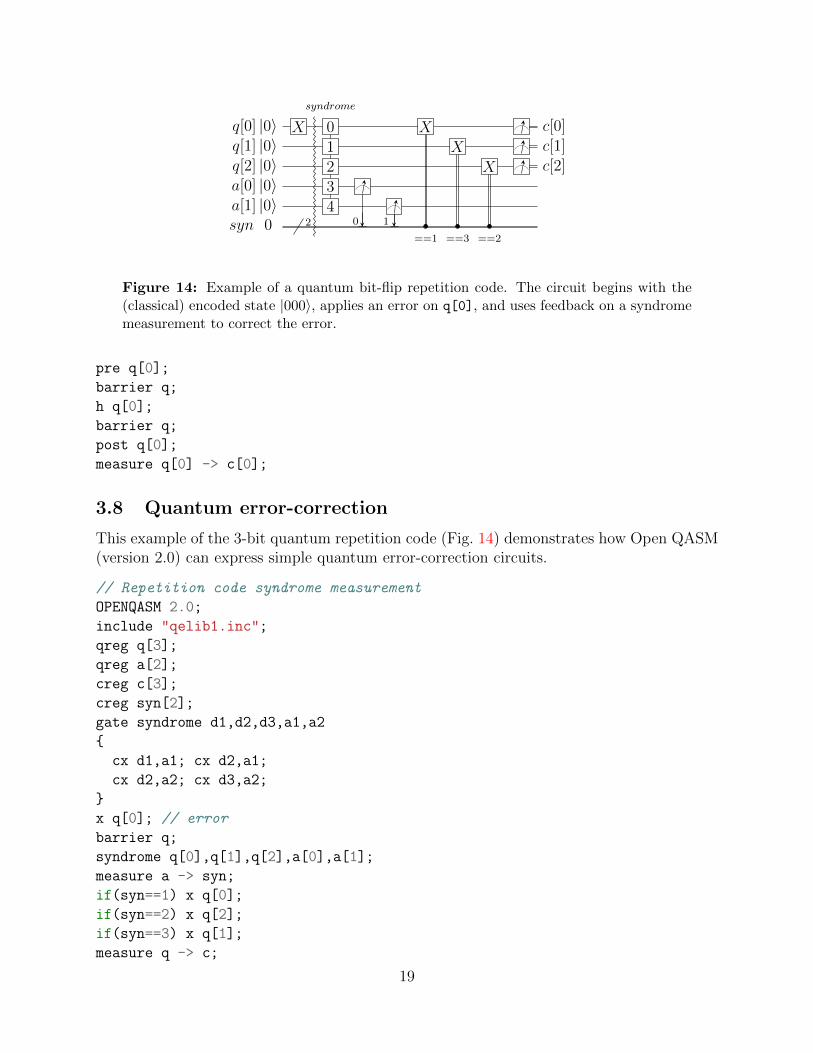
Figure 14: Example of a quantum bit-flip repetition code. The circuit begins with the(classical) encoded state |000〉, applies an error on q[0], and uses feedback on a syndromemeasurement to correct the error.

pre q[0];

barrier q;

h q[0];

barrier q;

post q[0];

measure q[0] -> c[0];

3.8 Quantum error-correction

This example of the 3-bit quantum repetition code (Fig. 14) demonstrates how Open QASM(version 2.0) can express simple quantum error-correction circuits.

// Repetition code syndrome measurement

OPENQASM 2.0;

include "qelib1.inc";

qreg q[3];

qreg a[2];

creg c[3];

creg syn[2];

gate syndrome d1,d2,d3,a1,a2

{

cx d1,a1; cx d2,a1;

cx d2,a2; cx d3,a2;

}

x q[0]; // error

barrier q;

syndrome q[0],q[1],q[2],a[0],a[1];

measure a -> syn;

if(syn==1) x q[0];

if(syn==2) x q[2];

if(syn==3) x q[1];

measure q -> c;

19

4 Acknowledgements

This document represents ideas and contributions from the IBM Quantum Computing groupas a whole. We acknowledge suggestions and discussions with the IBM Quantum Experiencecommunity [30]. We thank Abigail Cross for typesetting the figures and proof-reading thedocument. We thank Tom Draper and Sandy Kutin for the 〈q|pic〉 package [31], which wasused for initial typesetting of the quantum circuits. We acknowledge partial support fromthe IBM Research Frontiers Institute.

20

A Open QASM Grammar

〈mainprogram〉 |= OPENQASM 〈real〉 ; 〈program〉〈program〉 |= 〈statement〉 | 〈program〉 〈statement〉〈statement〉 |= 〈decl〉

| 〈gatedecl〉 〈goplist〉 }| 〈gatedecl〉 }| opaque 〈id〉 〈idlist〉 ;| opaque 〈id〉 ( ) 〈idlist〉 ; | opaque 〈id〉 ( 〈idlist〉 ) 〈idlist〉 ;| 〈qop〉| if ( 〈id〉 == 〈nninteger〉 ) 〈qop〉| barrier 〈anylist〉 ;

〈decl〉 |= qreg 〈id〉 [ 〈nninteger〉 ] ; | creg 〈id〉 [ 〈nninteger〉 ] ;

〈gatedecl〉 |= gate 〈id〉 〈idlist〉 {| gate 〈id〉 ( ) 〈idlist〉 {| gate 〈id〉 ( 〈idlist〉 )〈idlist〉 {

〈goplist〉 |= 〈uop〉| barrier 〈idlist〉 ;| 〈goplist〉 〈uop〉| 〈goplist〉 barrier 〈idlist〉 ;

〈qop〉 |= 〈uop〉| measure 〈argument〉 - > 〈argument〉 ;| reset 〈argument〉 ;

〈uop〉 |= U ( 〈explist〉 ) 〈argument〉 ;| CX 〈argument〉 , 〈argument〉 ;| 〈id〉 〈anylist〉 ; | 〈id〉 ( ) 〈anylist〉 ;| 〈id〉 ( 〈explist〉 ) 〈anylist〉 ;

〈anylist〉 |= 〈idlist〉 | 〈mixedlist〉〈idlist〉 |= 〈id〉 | 〈idlist〉 , 〈id〉

〈mixedlist〉 |= 〈id〉 [ 〈nninteger〉 ] | 〈mixedlist〉 , 〈id〉| 〈mixedlist〉 , 〈id〉 [ 〈nninteger〉 ]| 〈idlist〉 , 〈id〉[ 〈nninteger〉 ]

〈argument〉 |= 〈id〉 | 〈id〉 [ 〈nninteger〉 ]〈explist〉 |= 〈exp〉 | 〈explist〉 , 〈exp〉〈exp〉 |= 〈real〉 | 〈nninteger〉 | pi | 〈id〉

| 〈exp〉 + 〈exp〉 | 〈exp〉 - 〈exp〉 | 〈exp〉 * 〈exp〉| 〈exp〉 / 〈exp〉 | - 〈exp〉 | 〈exp〉 ^ 〈exp〉| ( 〈exp〉 ) | 〈unaryop〉 ( 〈exp〉 )

〈unaryop〉 |= sin | cos | tan | exp | ln | sqrt

21

This is a simplified grammar for Open QASM presented in Backus-Naur form. Theunlisted productions 〈id〉, 〈real〉 and 〈nninteger〉 are defined by the regular expressions:

id := [a-z][A-Za-z0-9_]*

real := ([0-9]+\.[0-9]*|[0-9]*\.[0-9]+)([eE][-+]?[0-9]+)?

nninteger := [1-9]+[0-9]*|0

Not all programs produced using this grammar are valid Open QASM circuits. As explainedin Section 2, there are additional rules concerning valid arguments, parameters, declara-tions, and identifiers, as well as the standard operator precedence rules in the parameterexpressions.

References

[1] P. Selinger. A brief survey of quantum programming languages. Proc. Seventh Int’lSymp. Functional and Logic Programming, pages 1–6, 2004.

[2] S. Gay. Quantum programming languages: survey and bibliography. Math. Structuresin Computer Science, 16:581–600, 2006.

[3] K. Svore, A. Cross, A. Aho, I. Chuang, and I. Markov. A layered software architecturefor quantum computing design tools. IEEE Computer, (39(1)):74–83, 2006.

[4] T. Haner, D. Steiger, K. Svore, and M. Troyer. A software methodology for compilingquantum programs. arxiv:1604.01401, 2016.

[5] D. Wecker and K. Svore. LIQUi|〉: A software design architecture and domain-specificlanguage for quantum computing. arXiv:1402.4467, 2014.

[6] LIQUi|〉: The Language Integrated Quantum Operations Simulator. http://stationq.github.io/Liquid/, 2016. accessed November 2016.

[7] A. JavadiAbhari, S. Patil, D. Kudrow, J. Heckey, A. Lvov, F. Chong, and M. Martonosi.ScaffCC: a framework for compilation and analysis of quantum computing programs.ACM International Conference on Computing Frontiers (CF 2014), 2014.

[8] Compilation, analysis and optimization framework for the Scaffold quantum program-ming language. https://github.com/epiqc/ScaffCC, 2016. accessed November 2016.

[9] B. Valiron, N. Ross, P. Selinger, D. Scott Alexander, and J. Smith. Programming thequantum future. Communications of the ACM, 58(8):52–61, 2015.

[10] The Quipper Language. http://www.mathstat.dal.ca/~selinger/quipper/, 2013.accessed November 2016.

[11] A. S. Green, P. LeFanu Lumsdaine, N. J. Ross, P. Selinger, and B. Valiron. Quipper:a scalable quantum programming language. ACM SIGPLAN Notices, (48(6)):333–342,2013.

22

[12] M. Troyer D. S. Steiger, T. Haner. ProjectQ: An open source software framework forquantum computing. arXiv:1612.08091, 2016.

[13] ProjectQ. https://projectq.ch, 2017. accessed January 2017.

[14] B. Omer. Structured quantum programming. Vienna University of Technology, Ph. D.thesis, 2003.

[15] B. Omer. QCL – a programming language for quantum computers. http://tph.

tuwien.ac.at/~oemer/qcl.html, 1998. accessed November 2016.

[16] G. Viamontes, H. Garcia, I. Markov, and J. Hayes. QuIDDPro: High-performancequantum circuit simulation. http://vlsicad.eecs.umich.edu/Quantum/qp/, 2004.accessed November 2016.

[17] G. F. Viamontes, I. L. Markov, and J. P. Hayes. Graph-based simulation of quantumcomputation in the density matrix representation. Quant. Inf. Comp., 5(2):113–130,2005.

[18] X. Liu and J. Kubiatowicz. Chisel-Q: designing quantum circuits with a Scala embeddedlanguage. IEEE 31st International Conference on Computer Design (ICCD), 2013.

[19] Chisel: constructing hardware in a Scala embedded language. https://chisel.eecs.

berkeley.edu/, 2016. accessed November 2016.

[20] Quil. https://github.com/rigetticomputing/pyquil, 2017.

[21] R. Smith, M. Curtis, and W. Zeng. A practical quantum instruction set architecture.arXiv:1608.03355, 2016.

[22] M. Nielsen and I. Chuang. Quantum computation and quantum information. CambridgeUniversity Press, 2000.

[23] I. Chuang. qasm2circ. http://www.media.mit.edu/quanta/qasm2circ/, 2005. ac-cessed November 2016.

[24] A. Cross. qasm-tools. http://www.media.mit.edu/quanta/quanta-web/projects/

qasm-tools/, 2005. accessed November 2016.

[25] S. Balensiefer, L. Kreger-Stickles, and M. Oskin. QUALE: quantum architecture layoutevaluator. Proc. SPIE 5815, Quantum information and computation III, (103), 2005.

[26] M. Dousti, A. Shafaei, and M. Pedram. Squash 2: a hierarchical scalable quantummapper considering ancilla sharing. Quant. Inf. Comp., 16((4)), 2016.

[27] A. Barenco, C. Bennett, R. Cleve, D. DiVincenzo, N. Margolus, P. Shor, T. Sleator,J. Smolin, and H. Weinfurter. Elementary gates for quantum computation. Phys. Rev.A, 52(3457), 1995.

[28] N. D. Mermin. Quantum Computer Science. Cambridge, 2007.

23

[29] S. Cuccaro, T. Draper, S. Kutin, and D. Moulton. A new quantum ripple-carry additioncircuit. arXiv:quant-ph/0410184, 2004.

[30] The IBM Quantum Experience. http://www.research.ibm.com/quantum/, 2016. ac-cessed November 2016.

[31] T. Draper and S. Kutin. 〈q|pic〉: Quantum circuit diagrams in latex. https://github.com/qpic/qpic, 2016. accessed November 2016.

24