1

Open Set Face Recognition Using Transduction

Fayin Li and Harry Wechsler

Department of Computer Science

George Mason University

Fairfax, VA 22030

{fli, wechsler}@cs.gmu.edu

Abstract: This paper motivates and describes a novel realization of transductive inference that can

address the Open Set face recognition task. Open Set operates under the assumption that not all the test

probes have mates in the gallery. It either detects the presence of some biometric signature within the

gallery and finds its identity or rejects it, i.e., it provides for the “none of the above” answer. The main

contribution of the paper is Open Set TCM – kNN (Transduction Confidence Machine – k Nearest

Neighbors), which is suitable for multi-class authentication operational scenarios that have to include a

rejection option for classes never enrolled in the gallery. Open Set TCM – kNN, driven by the relation

between transduction and Kolmogorov complexity, provides a local estimation of the likelihood ratio

needed for detection tasks. We provide extensive experimental data to show the feasibility, robustness, and

comparative advantages of Open Set TCM – kNN on Open Set identification and watch list (surveillance)

tasks using challenging FERET data. Last, we analyze the error structure driven by the fact that most of

the errors in identification are due to a relatively small number of face patterns. Open Set TCM - kNN is

shown to be suitable for PSEI (pattern specific error inhomogeneities) error analysis in order to identify

difficult to recognize faces. PSEI analysis improves biometric performance by removing a small number of

those difficult to recognize faces responsible for much of the original error in performance and/or by using

data fusion.

Key Words: biometrics, confidence, credibility, data fusion, information quality, Kolmogorov

complexity, face recognition, open set recognition, performance evaluation, PSEI (pattern specific

error inhomogeneities), randomness deficiency, strangeness, face surveillance, (multi-class)

transduction, watch list, clustering, outlier detection

2

1. Introduction

Face recognition (Chellappa et al., 1995; Daugman, 1997; Jain et al., 1999; Zhao et al., 2003; Bolle et

al., 2004; Liu and Wechsler, 2004) has become one of the major biometric technologies in use. The

generic open set recognition problem, a major challenge for face recognition, operates under the

assumption that not all the probes (unknown test face images) have mates (counterparts) in the

gallery (of known subjects). It requires the a priori availability of a reject option to answer “none

of the above”. If the probe is detected rather than rejected, the face recognition engine must then

identify / recognize the subject. The operational analogue for open set face recognition is the

(usually small) Watch List or Surveillance task, which involves (i) negative identification

(“rejection”) due to the obvious fact that the large majority [almost all] of the people screened at

security entry points are law abiding people, and (ii) correct identification for those that make up

the watch list.

Transduction, the (non-inductive) inference methodology proposed here to address the

challenges characteristic of the open set face recognition problem, is a type of local inference that

moves from particular to particular (Vapnik, 1998). It addresses the small sample size problem

that affects face recognition due to the lack of enough data for training and/or testing.

Transductive inference, in analogy to learning from unlabeled exemplars (Mitchell, 1999), is

directly related to the case when one has to classify some (unknown) test (probe) face images and

the choice is among several (tentative) classifications, each of them leading to different

(re)partitionings of the original ID(entity) face space. The paper introduces the Open Set TCM –

kNN (Transduction Confidence Machine – k Nearest Neighbors), which is a novel realization of

transductive inference that is suitable for open set multi-class classification. Open Set TCM –

kNN, driven by the relation between transduction and Kolmogorov complexity, provides a local

estimation of the likelihood ratio required for detection tasks and provides for the needed

3

rejection option. The paper provides extensive experimental data to show the feasibility,

robustness, and comparative advantages of Open Set TCM – kNN against existing methods using

challenging FERET data.

The outline for the paper is as follows. Sect. 2 familiarizes the reader with face recognition and

the protocols used. Sects. 3 and 4 discuss the learning theory behind transduction. In particular,

Sect. 4 describes the TCM (Transduction Confidence Machine) (Proedrou, 2001). Sect. 5

includes one of the main contributions of this paper, Open Set TCM-kNN. It expands on TCM

and provides for a novel transductive algorithm that is suitable for the open set multi-class

recognition problem that includes a rejection option. Sect. 6 describes the experimental design set

up, while Sects. 7 and 8 describe the use of Open Set TCM-kNN for open set and watch list /

surveillance biometric recognition tasks. Sects. 9 and 10 deal with error analysis and how to use

the uneven contributions to errors made by face patterns for effective data fusion. The conclusions

are presented in Sect. 11.

2. Face Recognition Tasks and Performance Evaluation Protocols

The generic (on-line) biometric system used herein is shown in Fig. 1. The match component

compares the biometric information extracted from the sample face exemplar and the signature

stored in the reference (signature) template(s). One has to compare then an output score with a

predefined threshold value. The comparison may be against a single template (for verification),

or against a list of candidate templates (for identification). The face space, i.e., the basis needed

to generate the templates, is derived using face images acquired ahead of time and independent of

those that would be later on enrolled or tested (see top of Fig. 1).

FERET (Phillips et al., 1998) and BANCA (Bailly-Bailliere et al., 2003), the standard

evaluation protocols in use today, are briefly described next. FERET undertakes algorithmic

(technology) and scenario evaluations. It works by considering target (gallery) T and query

4

(probe) Q sets. The output for FERET is a full (distance) matrix S (q, t), which measures the

similarity between each query, q ∈ Q, and each target, t ∈ T, pair. The nearest neighbor (NN)

classifier authenticates then face images using the similarity scores recorded by S. The availability

of the matrix S allows for different “virtual” experiments to be conducted when one selects the

specific query P and gallery G as subsets of Q and T.

Figure 1. Face Recognition Methodology

User faces

Quality checker

Feature Extractor

System DB

Template name

Enrollment

User faces

Feature Extractor

Matcher (1 match)

System DB

One template

Verification True/False

Claimed identity

User faces

Feature Extractor

Matcher (N matches)

System DB

N templates

Identification User’s identity or

“user non identified”

Face Space Basis Derivation

5

The 1 : N open set problem referred to by FRVT2002 (Phillips et al., 2003) as the watch list

task, is briefly addressed by FRVT2002 after the two (degenerate) special cases of verification

and closed set identification. Verification corresponds to an open set identification for a gallery

size of N = 1, while closed set identification seeks the match for an image whose mate is known to

be in the gallery, i.e., for each image probe p ∈ P there exists (exactly one) gallery mate g* ∈ G.

Cumulative Matching Curves (CMC) and Receiver Operating Characteristics (ROC), used to

display both closed and open set, are derived for different thresholds but using ground truth,

which would not be available during field operation.

The closed universe model for 1 : N identification is quite restrictive as it does not reflect the

intricacies for the actual real positive and negative identification scenarios. Under positive claim of

identity, the user claims to be enrolled in or to be on the watch list, while under negative claim of

identity the user claims not to be enrolled or known to the system. “Performance for the open set

problem is quantified over two populations. First the impostors, those persons who are not

present in the gallery, i.e., not on the watch list, are used to compute the false match [acceptance]

rate, which is needed to quantify rejection capability. Second, for those persons who are “known”

(i.e., previously enrolled) to a system, the open set identification rate, is used to quantify user [hit]

performance” (Grother, 2004).

The use of the open set concept by the BANCA protocol is quite restricted. It only refers to

the derivation of the feature (face) space and the parameters needed for verification. We referred

to this earlier as face space basis derivation (see top of Fig. 1). BANCA protocol, however,

does not address the full scope of open set identification, where some probes are not mated in the

gallery.

3. Transduction

6

Transductive inference is a type of local inference that moves from particular to particular

(Vapnik, 1998; 2000) (see Fig. 2). “In contrast to inductive inference where one uses given

empirical data to find the approximation of a functional dependency (the inductive step [that

moves from particular to general]) and then uses the obtained approximation to evaluate the

values of a function at the points of interest (the deductive step [that moves from general to

particular]), one estimates [using transduction] the values of a function [only] at the points of

interest in one step” (Vapnik, 1998). The simplest mathematical method for transductive

inference is the method of k nearest neighbors. The Cover – Hart (1967) theorem proves that

asymptotically the one nearest neighbor algorithm is bounded above by twice the Bayes minimum

probability of error. Cover and Hart also showed that the k-NN error approaches the Bayes error

(with factor 1) if k = Θ(log n).

Figure 2. Transduction [Vapnik, 2000]

Vapnik (1998) approaches transductive inference as follows. Given training (labeled)

exemplars one seeks among feasible labelings of the (unlabeled probe) test exemplars the one

that makes the error observed during testing (labeling) consistent with the error recorded during

training. It is also assumed that the training and test exemplars are i.i.d according to some

[common] distribution function. Vapnik (1998) defines then the overall risk functional using two

equivalent settings with the explicit goal of minimizing them.

7

Setting #1 says “Given a small sample size set of training sample exemplars, T, which consists of

l pairs (xi, yi), estimate the value of the function y = Φ (x) at the given [working test probe sample

exemplars] set W of points xl + 1,..., xl + m. (Size l is considered to be small if the ratio l / h is small,

say l / h < 20, where h is the VC-dimension of the set). Based on the training set T, the working

set W, and on a given set of functions f (x,α), α ∈ Λ [Φ (x) does not necessarily belong to this

set], find f (x,α*) that minimizes with a preassigned probability 1 – η the overall risk of forecasting

the values of the function yi = Φ (xi) on the elements of the working set W -- that is, which yields

with probability 1 – η a value of the functional

∑=

++=m

iilil xfy

mR

1

)),(,(1

)( αρα (1)

close to the minimal one”. ρ(y, f (x, α)) is some measure of discrepancy between y and f (x, α), say

ρ(yl + i, f (xl + i, α)) = (yl + i - f (xl + i, α))2 (2)

Setting #1 seeks to minimize the deviation between the risk on the training and working samples.

Setting #2 considers training and working samples [chosen according to a probability distribution

function P(x, y)], and seeks an algorithm A that will choose a function f (x, αA),

f (x, αA) = f (x, αA (x1, y1;…; xl , yl; xl + 1, … , xl + m)) (3)

that yields the value of the functional

∫ ∑+

+=++=

ml

limllllAii xxdPyxdPyxdPxfy

mAR

1111 ),,(),(),())),(,(

1()( KKαρ (4)

close to the minimal one, when the sum Σ is indexed for (unlabeled) exemplars i between l + 1

and l + m. Setting #2 labels W, the working exemplars set, in a fashion consistent with T, the

training set, e.g., using minimization for some error functional over T ∪∪∪∪ W. One possible

realization using SVM (support vector machines) is to classify the joint set of training and

working exemplars with maximal margin over all possible classifications L(W) for the working

set W, e.g., arg min L (W) min w 1 / 2 || w || 2 (Saunders et al., 1999).

8

The solutions for Settings #1 and #2 are connected (Theorem 8.1) (Vapnik, 1998). An

example is TSVM (Transductive inference using SVM), which has been shown to yield substantial

improvements for text classification, a two-class classification task, over inductive methods,

especially for small training sets and large test (working) sets. The observed success was

explained due to the fact that “the margin of separating hyperplanes is a natural way to encode

prior knowledge for (text) classifiers and to study the location of text exemplars (with respect to

the hyperplane), which is not possible for an inductive learner” (Joachims, 1999).

The goal for inductive learning is to generalize for any future test set, while the goal for

transductive inference is to make predictions for a specific working set. The working exemplars

provide additional information about the distribution of data and their explicit inclusion in the

problem formulation yields better generalization on problems with insufficient labeled points

(Gammerman et al., 1998). Transductive inference becomes suitable for face recognition when

some of the faces available for training lack proper ID(entification) or when one has to classify

some (unknown) test face image(s). The challenge is to choose among several (tentative)

classifications, each of them leading to different partitionings of the ID(entity) face space. The

scope for transducive inference is augmented herein in order to cope with the open set recognition

problem, which requires (a) detection in addition to mere identification; and (b) the ability to cope

with multi-class rather than two-class classification. The solution to this problem is presented in

the next two sections.

4. Kolmogorov Complexity and Randomness Deficiency

There is a strong connection between transductive inference and Kolmogorov complexity. Let

#(z) be the length of the binary string z and K(z) its Kolmogorov complexity, which is the length

of the smallest program (up to an additive constant) that a Universal Turing Machine needs as

input in order to output z. The randomness deficiency D(z) for string z (Li and Vitanyi, 1997;

9

Vovk et al., 1999) is

D(z) = #( z) – K(z) (5)

and it measures how random is the binary string z and the set it represents. The larger the

randomness deficiency is, the more regular and more probable the string z is (Vovk et al., 1999).

[Another connection between Kolmogorov complexity and randomness is via MDL (minimum

description length).] Transductive inference seeks to find from all possible labelings L(W) the one

that yields the largest randomness deficiency, i.e., the most probable labeling. This choice models

the working (“test”) exemplar set W in a most similar fashion to the training set T and would

thus minimally change the original model for T or expand it for T ∪ W (see Sect. 3 for the

corresponding transductive settings). “The difference between the classifications that induction

and transduction yield for some working exemplar approximates its randomness deficiency. The

intuitive explanation is that we disturb a classifier (driven by T) by inserting a new working

examplar in a training set. A magnitude of this disturbance is an estimation of the classifier’s

instability (unreliability) in a given region of its problem space” (Kukar and Kononenko, 2002).

Randomness deficiency is, however, not computable (Li and Vitanyi, 1997). One has to

approximate it instead using a slightly modified Martin- Löf test for randomness and the values

taken by such randomness tests are called p-values. The p-value construction used here has been

proposed by Gammerman et al. (1998) and Proedrou et al. (2001). Given a sequence of distances

from exemplar i to other exemplars, the strangeness of i with putative label y is defined as:

1k

1j

yij

k

1j

yiji ddα

−

=

−

=

= ∑∑ (6)

The strangeness measure iα is the ratio of the sum of the k nearest distances d from the same

class (y) divided by the sum of the k nearest distances from all the other classes (–y). The

strangeness of an exemplar increases when the distance from the exemplars of the same class

10

becomes larger and when the distance from the other classes becomes smaller. The smaller the

strangeness the larger its randomness deficiency is. Note that each new test exemplar e with

putative label y and derived strangeness ynewα requires to recompute, if necessary, the strangeness

for all the training exemplars when the identity of their k nearest neighbors exemplars changes due

to the location of (the just inserted new exemplar) e.

The p-value construction shown below, where l is the cardinality of the training set T,

constitutes a valid randomness (deficiency) test approximation (Melluish et al., 2001) for this

tranductive (putative label y) hypothesis.

1

):{#)(

+≥=

l

iep

ynewi

y

αα (7)

An alternative valid randomness (deficiency) approximation (Vovk et al., 1999) and the one that

we use here defines the p-value for a working exemplar e (with putative label y) as:

)()1()()()()(

)( 21y

new

ynewl

yαfl

αfαfαfαfep

+++++= L

(8)

where the function f used is monotonic non-decreasing with f(0) = 0, and l is the number of

training exemplars. Experimental data reported later in this paper uses f(α) = α. Our empirical

evidence has shown that the alternative randomness approximation (8) yields better performance

than the standard one (7), which may suffer from “distortion phenomenon” (Vovk et al., 1999). If

there are c classes in the training data, there are c p-values for each working exemplar e. Using p-

values one chooses that particular labeling driven by the largest randomness deficiency for class

membership, i.e., the putative label y that yields the least strangeness or correspondingly the

largest p-value. This largest p-value is also defined as the credibility of the label chosen, which is

a measure of information quality. The associated confidence measure, which is derived as the 1st

largest p-value (or one) minus the 2nd largest p-value, indicates how close the first two

11

assignments are. The confidence value indicates how improbable classifications other than the

predicted labeling are, while the credibility value shows how suitable the training set is for the

classification of that working exemplar.

The transductive inference approach uses the whole training set T to infer a rule for each new

exemplar. Based on the p-values defined above, Proedrou et al. (2001) have proposed the TCM-

kNN (Transduction Confidence Machine - k Nearest Neighbor) to serve as a formal transduction

inference algorithm for classification purposes. TCM-kNN has access to a distance function d

that measures the similarity between any two exemplars. Different similarity measures (see Sect.

6) are used and their relative performance varies accordingly. TCM-kNN does not address,

however, the detection (decision) aspect needed for open set face recognition. Our proposed

solution for the detection aspect involves using the PSR (peak-side-ratio) that characterizes the

distribution of p-values. It implements the equivalent of the likelihood ratio (LR) used in

detection theory and hypothesis testing, where LR is the ratio between the hypothesis H0 that the

unknown probe belongs to the gallery and H1 (alternative hypothesis) that it does not belong.

The distribution for the PSR, if impostor cases were made available, serves to determine how

to threshold in order to accept or reject a particular working exemplar e. Towards that end, one

would relabel the training exemplars, one at a time, with all putative labels except the one

originally assigned to it. The corresponding PSR should resolve each such relabeled exemplar

suitable for rejection because its new label is mistaken. The resulting distribution for the PSR

determines then when to reject working exemplars as impostors. Open Set TCM – kNN

implements the above concepts and it is described in the next section.

5. Open Set TCM-kNN

Open Set recognition operates under the assumption that not all the probes have mates in the

gallery and it thus requires the reject option. Given a new (test / probe) working exemplar e, the

12

p-values output from Open Set TCM-kNN records the likelihoods that the new exemplar comes

from each putative subject in the training data. If some p-value is high enough and it significantly

outscores the others, the new exemplar can be mated to the corresponding subject ID with

credibility p. If the top ranked (highest p-values) choices are very close to each other and outscore

the other choices, the top choice can still be accepted but its recognition is questionable due to

ambiguity and yields low confidence. The confidence measures the difference between the 1st and

2nd largest (or consecutive) p-values. If all p-values are randomly distributed and no p-values

outscore other p-values enough, any recognition choice will be questionable and the new

exemplar should be rejected. The proposed PSR (peak-to-side ratio)

PSR = (pmax – pmean) / pstdev (9)

characterizes those characteristics of p-value distribution, where pmean and pstdev are the mean

and standard deviation of the p-value distribution without pmax.

The threshold for rejection is learned a priori from the composition and structure of the training

data set at enrollment time. Each training exemplar e is iteratively reassigned to all possible

classes but different from its own and the p-values are recomputed accordingly. The PSR is

derived using the recomputed p-values with e playing the role of an impostor. The PSR values

found for such impostors are low (since they do not mate) compared to those derived before for

legitimate subjects and they require rejection. The PSR distribution (and its tail) provides a robust

method for deriving a priori the operational threshold Θ for detection as

Θ = PSRmean + 3 × PSRstdev (10)

where PSRmean and PSRstdev (standard deviation) are characteristic for the PSR distribution. The

probe is then rejected if the relationship PSRnew ≤ Θ holds true. Correspondingly, authentication

takes place for (large) values exceeding Θ.

13

There are conceptual similarities between the use of the PSR to approximate the likelihood

ratio and scoring normalization methods used in speaker verification (Furui, 1997; Reynolds et al.,

2000). The alternative hypothesis for speech is modeled using either the cohort or the universal

background model (UBM). The cohort approximates the alternative H1 hypothesis using speech-

specific (same gender impostor) subjects, while UBM models H1 by pooling speech from several

speakers and training a single speaker background model. The PSR measure is conceptually

related to the cohort model, as both implement LR using local estimation for the alternative

hypothesis. The ability of the cohort model to discriminate the speaker’s speech from those of

similar, same gender impostors is much better than that offered by UBM (Mak et al., 2001) and it

leads to improved security at lower FAR (false acceptance rates). Similar arguments hold for

other modalities, including human faces.

6. Experimental Design

The data set (see Fig. 3) from FERET (Phillips et al., 1998) consists of 750 frontal face images

corresponding to 250 subjects. 200 subjects come from the difficult batch #15 that was acquired

using variable illumination and/or facial expressions, while the remaining different 50 subjects

consists of are drawn from other batches. . Each subject has three normalized (zero mean and

unit variance) images of size 150 x 150 with 256 gray scale levels. Each column in Fig. 3

corresponds to one subject. The normalized 300 face images from 100 subjects are used to

generate PCA and FLD (Fisher Linear Discriminant) face basis (see top of Fig. 1). 50 subjects are

randomly selected from batch #15 and the remaining different 50 subjects were drawn from other

batches. The remaining 450 face images for 150 subjects are used for enrollment and testing.

They are projected on the PCA and FLD face bases derived ahead of time to yield 300 PCA

coefficients and 100 Fisherfaces using FLD on the reduced 300 PCA space (Liu and Wechsler,

2002). For each subject, two images are randomly selected as training and the third one as testing.

14

Figure 3. Face Images

We have used several well-known similarity measures (see below) to evaluate their effect on

different face representation (PCA and Fisherfaces) when using TCM-kNN (k=1). The similarity

distances d used are shown next. Given two n-dimensional vectors nYX ℜ∈, , the distance

measures used are defined as follows:

∑=

−=−=n

i

iiL YXYXYXd1

1 ),( )()(),(2

2 YXYXYXYXd TL −−=−=

YX

YXYXd

T

−=),(cos

YYXX

YX

YX

YXYXd

TT

TT

Dice +−=

+−= 22

),(22

YXYYXX

YX

YXYX

YXYXd

TTT

T

T

T

Jaccard −+−=

−+−=

22),(

)()(),( 12 YXYXYXd T

LMah −Σ−= −+

YX

YXYXd

T

Mah

1

cos ),(−

+Σ−=

where Σ is the covariance matrix of the training data. For PCA, Σ is diagonal and the diagonal

elements are the (eigenvalues) variances of the corresponding components. The Mahalanobis + L1

distance defined only for PCA is

∑=

+

−=

n

i i

iiLMah

YXYXd

11 ),(

λ

L1 defines the city-block distance, L2 defines the Euclidean distance. Cosine, Dice, Overlap and

Jaccard measure the relative overlay between two vectors. L1, L2 and cosine can also be weighted

by the covariance matrix of training data, which leads to Mahalanobis related distances. Our

empirical findings indicate that Mahalanobis related similarity distances are superior to others

15

when expressive features (driven by PCA) are used; while overlay related similarity distances are

superior when discriminating (Fisherfaces) features are used.

Figure 4. Generic Open Set and Watch List Tasks

The next two sections present experimental data that illustrates the usefulness and robustness

of Open Set TCM – kNN for (generic) open set face recognition and watch list tasks (see Figs.

4a and 4b, respectively). Watch list, a special task for open set face recognition, corresponds to

the case when the overlap between the gallery and probe sets is the gallery (watch list) itself and

the probe set size is much larger than the gallery. Open set and watch list can be thought

operationally relevant to the US-VISIT program where applicants are matched against large data

bases to possibly avoid repeat visa applications, while watch list corresponds to the case where

subjects are matched for negative identification against some WANTED list.

7. Open Set Face Recognition

Biometric systems in general, and face recognition engines, in particular, require significant tuning

and calibration, for setting the detection thresholds among other things, before “plug and play”.

Setting thresholds is not easy to automate due to their strong dependency on image quality and

the composition of training data. Note also that “much more is known about the population, [or

genuine customers,] of an application than is known about the enemies, [i.e., the imposters that

have to be rejected]. Consequently, the probability of a false alarm rate (FAR), a false match [for

16

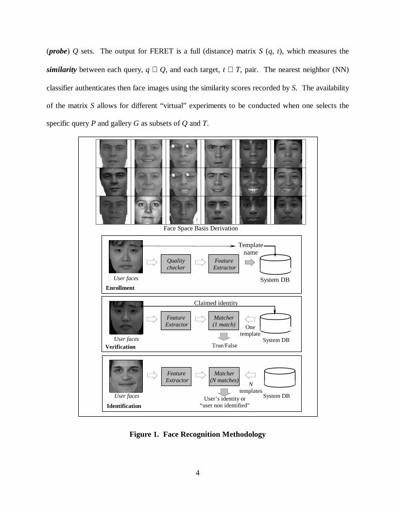
screening and positive identification], is hard to estimate. Hence, the false reject rate (FRR), that

concerns open set negative identification, is easier to estimate than the false alarm rate, because

the biometric samples of the enemy population are not available” (Bolle et al., 2004). The

thresholds needed for field deployment have to be set up ahead of time, i.e., a priori, and without

resorting to additional client, e.g., impostor data. The alternative of setting the thresholds a

posteriori using the ground truth available from the aggregate similarity scores recorded for

matching the probe set against the gallery set is not appropriate because the ground truth is not

available.

Conventional threshold selection methods typically compute the distribution of inter- and intra

ID (subject) distances, and then choose a threshold to equalize the overlapping areas of the

distributions, i.e., to equalize the false acceptance rate (FAR) and false rejection rate (FRR). “The

success of this approach, however, relies on whether the estimated distributions match the

subject- and impostor-class distributions. Session-to-session ID variability, however, contributes

much bias to the thresholds, rendering the authentication system unstable” (Bengio et al., 2001).

Comparative performance of Open Set TCM – kNN against Open Set {PCA, Fisherfaces}, the

corresponding versions for PCA and Fisherfaces, which are standard and well known face

recognition methods, is presented next. The face space basis derivation is done before enrollment

(see Fig. 1), the corresponding data collection was described in Sect. 6, and nearest neighbor

identification is done using the distances described in the previous section. Detection thresholds

for Open Set TCM – kNN are found as described in Sect. 5, while detection thresholds for Open

Set {PCA and Fisherfaces} are found as explained next.

The Open Set standard PCA (“Eigenfaces”) and Fisherfaces classifiers derive their rejection

threshold from the intra- and inter-distance (similarity) distribution of training exemplars in a

fashion similar to that used by FRVT2002. The statistics of intra-distance (“within”) distribution

17

set the lower bound of the threshold and the statistics of inter-distance (“between”) distribution

set the upper bound. As the minimum distance of the new (test / probe) exemplar to the

prototypes for each class becomes closer to or larger than the upper bound, the more likely the

new testing exemplar will be rejected. Our experiments have shown that face recognition

performance varies according to the threshold chosen.

The recognition rate reported is the percentage of subjects whose probe is correctly

recognized or rejected. Faces are represented using either 300 PCA or 100 Fisherfaces

components. From the 150 subjects available (see Sect. 6), 80 subjects are randomly selected to

form a fixed gallery, while another 80 subjects are randomly selected as probes such that 40 of

them have mates in the gallery, i.e, the gallery and probe sets have an overlap of 40 subjects. The

gallery consists of two (out of 3) randomly selected images; while the probes consist of the

remaining one (out of 3) images for faces that belong to the gallery and one (out of 3) randomly

selected image for subjects that do not belong to the gallery. During testing, all distance

measurements from Sect. 6 are used and the threshold varies from lower to upper bound. The

same experiment is run 100 times for different probe sets. The distance measurements d for Open

Set {PCA and Fisherfaces} that yield the best results are Mahalanobis + L2 and cosine,

respectively. Fig. 5 shows the mean recognition rate for different thresholds. When ground truth is

available the thresholds Θ are optimally set to yield maximum performance, and the reject

decision is taken if (min) d > Θ reject. The best average (over 100 experiments) authentication

(correct rejection and identification) rates (see Fig. 5) for Open Set {PCA, Fisherfaces} classifiers

that yield FAR = 7% are:

• 74.3% (s.d. = 3.06%) for PCA representation and sometime the optimal Θ ~ (Intramean ×

Intrastdev + Intermean × Interstdev)/(Interstdev + Intrastdev)

18

• 85.4% (s.d. = 2.30%) for Fisherfaces representation and sometime the optimal Θ ~

(Intramean × Interstdev + Intermean × Intrastdev)/(Interstdev + Intrastdev).

Figure 5. The Recognition Rate vs Threshold: PCA (Left) and Fisherfaces (Right)

For Open Set PCA, the results are very close if the number of components used varies from

150 to 300, while for Open Set Fisherfaces, the results are very close if the number of

components used varies from 55 to 90. More experiments have been done randomly varying the

gallery set and similar results were obtained. The optimal threshold, however, varies largely with

the gallery set and probe, and would be hard to be determined a priori. Attempts made to learn

the threshold a priori, i.e., without ground truth knowledge were unsuccessful.

Figure 6. PSR Histogram for PCA (Left) and Fisherfaces (Right) Components

The same Open Set experiment was run then using Open Set TCM – kNN for k = 1. The only

difference now is that the rejection threshold Θ is computed a priori according to the PSR

19

procedure described in Sect. 5 (see Fig. 6) Authentication is driven by large PSR and the average

authentication (correct rejection and identification) rates for (measured) FAR = 6% are:

• 81.2% (s.d. = 3.1%) for PCA using Θ = 5.51 and the Mahalanobis + L2 distance;

• 88.5% (s.d. = 2.6%) for Fisherfaces using Θ = 9.19 and the cosine distance.

Using PCA, the results for Open Set TCM-kNN are very close if the number of components used

varies from 170 to 300, while using Fisherfaces the results for Open Set TCM-kNN are very close

if the number of components used varies from 55 to 80. More experiments have been done

randomly varying the gallery set and similar results are obtained. The threshold varies with the

chosen gallery set and is determined a priori. This is different from Open Set {PCA, Fisherfaces}

where the performance shown is obtained only if the thresholds were optimally set a posteriori

using ground truth. Keeping this significant difference in mind, Open Set TCM-kNN outperforms

the Open Set {PCA, Fisherface} classifiers. Attempts to set the thresholds ahead of time (“a

priori”) for the Open Set {PCA, Fisherfaces} classifiers were not successful, because the intra–

and inter– distance distributions for the gallery are not too powerful to characterize the behavior

of the probe.

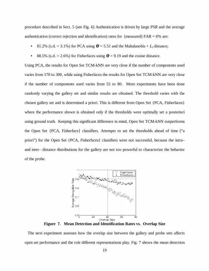
Figure 7. Mean Detection and Identification Rates vs. Overlap Size

The next experiment assesses how the overlap size between the gallery and probe sets affects

open set performance and the role different representations play. Fig. 7 shows the mean detection

20

and recognition rates for Open Set TCM – kNN using PCA and Fisherfaces representations, and

the Mahalanobis + L2 and cosine distances, respectively. There are 150 subjects available, the size

for both the gallery and the probe sets is 75 subjects, and the overlap between the gallery list and

the probe set varies from 0 to 75 subjects. We report the average results obtained over 100

randomized (over gallery and probe composition) runs. The performance goes down, almost

linearly, as the overlap size increases. Fisherfaces components yield overall much better

performance compared to PCA components, except for very small overlap size when the

performance observed is closed but still better when using Fisherfaces than PCA components. The

explanation for the observed performance is that as the size of overlap increases, it becomes more

difficult to detect and identify individuals on overlap set. The performance for the Open Set

{PCA, Fisherfaces} classifiers was very poor.

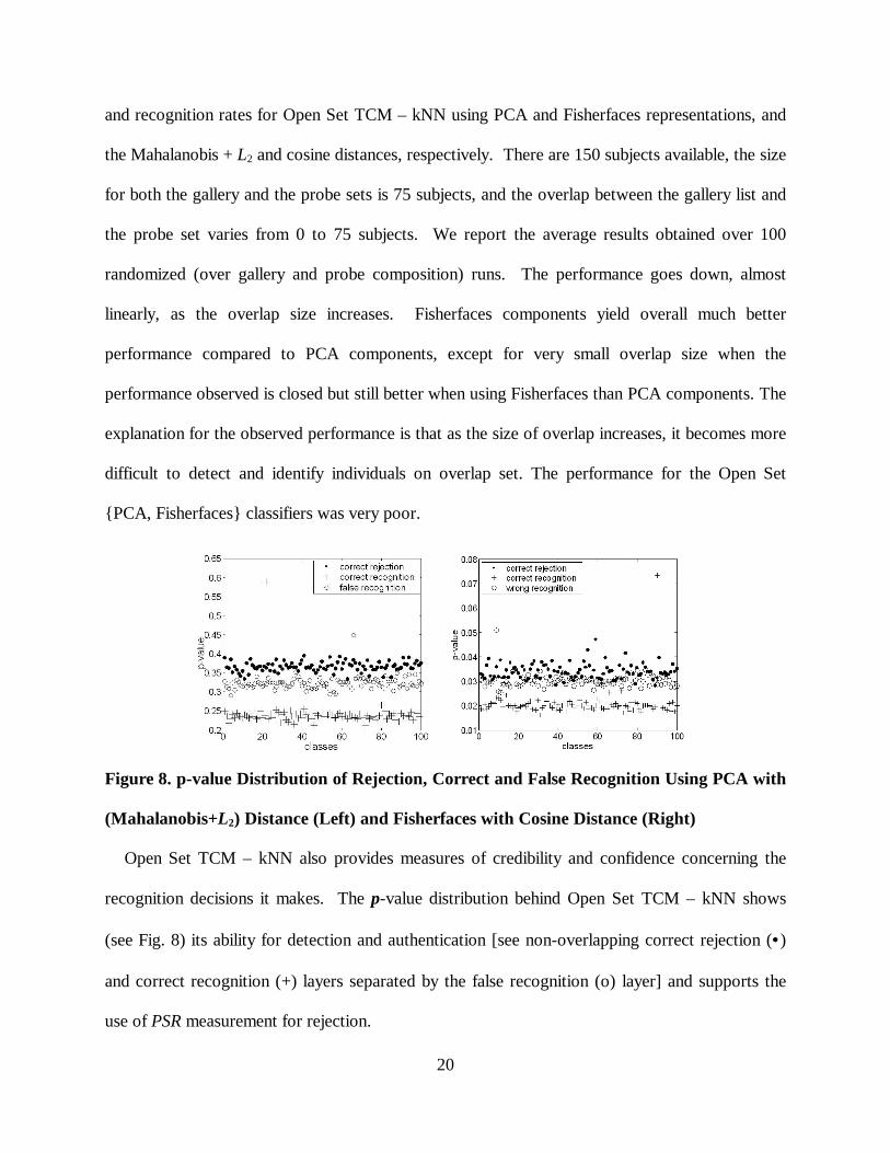
Figure 8. p-value Distribution of Rejection, Correct and False Recognition Using PCA with

(Mahalanobis+L2) Distance (Left) and Fisherfaces with Cosine Distance (Right)

Open Set TCM – kNN also provides measures of credibility and confidence concerning the

recognition decisions it makes. The p-value distribution behind Open Set TCM – kNN shows

(see Fig. 8) its ability for detection and authentication [see non-overlapping correct rejection (•)

and correct recognition (+) layers separated by the false recognition (o) layer] and supports the

use of PSR measurement for rejection.

21

8. Watch List

The gallery of wanted individuals is now very small compared to the number of people expected

to flood the biometric system (see Fig. 4b). People not on the watch list are “impostors” like,

whose negative identification is sought after. The next experiment reported has 150 subjects,

three images from each subject, for a total of 450 face images. We compare the Open Set {PCA,

Fisherfaces} and Open Set TCM - kNN classifiers on small watch lists (“galleries”), whose size

varies from 10 to 40 subjects, and reports the mean (average) performance (detection and

identification) rates obtained over 100 randomized runs. Let the watch list size be n subjects,

each of them having 2 (two) images in the gallery. Then there are 450 – 2n face images in the

probe set, n stands for the number of subjects on the watch list and 3 × (150 - n) stands for the

number of face images that come from subjects that are not on the watch list. The small size of

the watch list requires for stability purposes that the rejection threshold be derived from larger

populations but still using as before the same statistics of intra- and inter-distance distribution for

Open Set {PCA, Fisherfaces} and PSR distribution for Open Set TCM-kNN. The decision

thresholds Θ are derived in a manner similar to that used by cohort models in speech (see Sect. 5)

by augmenting the gallery with different subjects randomly drawn from other FERET batches

that include illumination and facial expression variation. The size of the gallery used to determine

the threshold is kept constant at 80 throughout the runs so the number 80 – n of different subjects

needed to augment it varies according to the size i of the watch list.

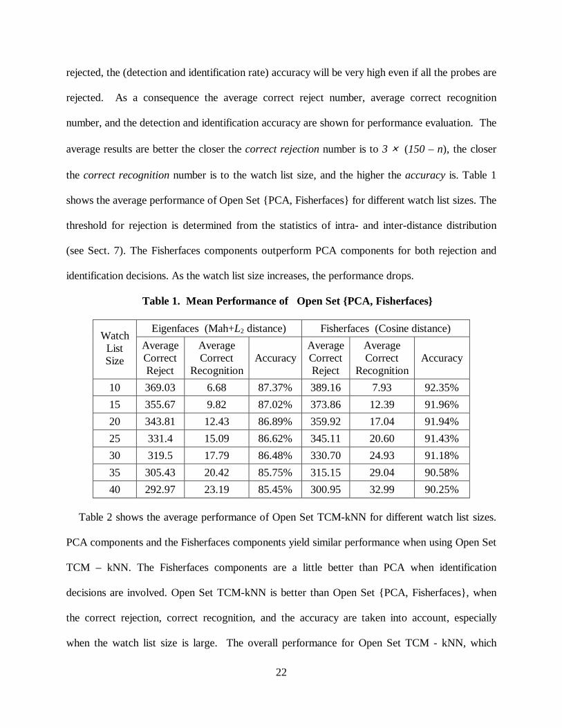
Table 1 and 2 shows the mean performance of Open Set {PCA, Fisherfaces} and Open Set

TCM - kNN for different watch list sizes. For watch list size n, the accuracy (detection and

identification rate) is (average correct rejection + average correct recognition) / (450 – 2n). The

numerical results, when the number of subjects on the watch list is n, should be interpreted as

follows. Since the watch list size is much smaller than the number of subjects that should be

22

rejected, the (detection and identification rate) accuracy will be very high even if all the probes are

rejected. As a consequence the average correct reject number, average correct recognition

number, and the detection and identification accuracy are shown for performance evaluation. The

average results are better the closer the correct rejection number is to 3 × (150 – n), the closer

the correct recognition number is to the watch list size, and the higher the accuracy is. Table 1

shows the average performance of Open Set {PCA, Fisherfaces} for different watch list sizes. The

threshold for rejection is determined from the statistics of intra- and inter-distance distribution

(see Sect. 7). The Fisherfaces components outperform PCA components for both rejection and

identification decisions. As the watch list size increases, the performance drops.

Table 1. Mean Performance of Open Set {PCA, Fisherfaces}

Eigenfaces (Mah+L2 distance) Fisherfaces (Cosine distance) Watch List Size

Average Correct Reject

Average Correct

Recognition Accuracy

Average Correct Reject

Average Correct

Recognition Accuracy

10 369.03 6.68 87.37% 389.16 7.93 92.35%

15 355.67 9.82 87.02% 373.86 12.39 91.96%

20 343.81 12.43 86.89% 359.92 17.04 91.94%

25 331.4 15.09 86.62% 345.11 20.60 91.43%

30 319.5 17.79 86.48% 330.70 24.93 91.18%

35 305.43 20.42 85.75% 315.15 29.04 90.58%

40 292.97 23.19 85.45% 300.95 32.99 90.25%

Table 2 shows the average performance of Open Set TCM-kNN for different watch list sizes.

PCA components and the Fisherfaces components yield similar performance when using Open Set

TCM – kNN. The Fisherfaces components are a little better than PCA when identification

decisions are involved. Open Set TCM-kNN is better than Open Set {PCA, Fisherfaces}, when

the correct rejection, correct recognition, and the accuracy are taken into account, especially

when the watch list size is large. The overall performance for Open Set TCM - kNN, which

23

keeps almost constant as the watch list size increases, is thus more stable than the overall

performance displayed by Open Set {PCA, Fisherfaces}.

Table 2. Mean Performance of Open Set TCM-kNN

Eigenfaces (Mah+L2 distance) Fisherfaces (Cosine distance) Watch List Size

Average Correct Reject

Average Correct

Recognition Accuracy

Average Correct Reject

Average Correct

Recognition Accuracy

10 389.74 7.64 92.41% 393.08 8.48 93.62%

15 376.28 11.72 92.38% 380.24 12.16 93.43%

20 364.18 14.12 92.27% 365.28 16.16 93.03%

25 350.24 18.26 92.13% 351.84 19.56 92.85%

30 336.94 21.62 91.94% 335.72 25.52 92.63%

35 322.96 25.22 91.63% 322.28 29.36 92.54%

40 309.24 27.98 91.14% 308.64 33.28 92.41%

The difference in performance between Fig. 7 and Table 2 indicates that the gallery size is also

an important factor affecting algorithm performance. In Fig. 7 the gallery (watch list) size is

always 75 subjects and only the overlap size between the gallery and probe sets changes, while in

Table 2 the gallery size (watch list) varies according to n.

9. Pattern Specific Error Inhomogeneities Analysis (PSEI)

It is important to know not only what works and to what extent it works, but also to know what

does not work and why (Pankanti et al., 2002). Anecdotal evidence suggests that 90% of errors

are due to only 10% of the face patterns. The contribution made by face patterns to the overall

system error is thus not even. Characterization of individual contributions to the overall face

recognition system error has received, however, little attention.

Pattern Specific Error Inhomogeneities (PSEI) analysis (Doddington et al, 1998) shows that

the error rates vary across the population. It has led to the jocular characterization of the target

population as being composed of “sheep” and “goats”. In this characterization, the sheep, for

24

whom authentication systems perform reasonably well, dominate the population, whereas the

goats, though in a minority, tend to determine the performance of the system through their

disproportionate contribution of false reject errors. Like targets, impostors also have barnyard

appellations, which follow from inhomogeneities in impostor performance across the population.

Specifically there are some impostors who have unusually good success at impersonating many

different targets. These are called “wolves”. There are also some targets that are easy to imitate

and thus seem unusually susceptible to many different impostors. These are called “lambs”.

ROC can be improved if some of the most difficult data (e.g., the “goats”, the hard to match

subjects) were excluded and/or processed differently. In general, if the tails of the ROC curve do

not asymptote at zero FAR and zero FRR, there is probably some data that could be profitably

excluded and maybe processed offline. The trick is to find some automatic way of detecting these

poor data items (Bolle et al., 2004) and adopt solutions different from “one size fits all”.

We describe next our approach for PSEI analysis that divides the subjects’ faces into

corresponding “barnyard” classes. The analysis of the error structure in terms of rejection and

acceptance decisions follows that of Pankanti et al. (2002) for fingerprints but is driven here by

transduction and applied to open set face recognition. There are low matching PSR scores X

that, in general, do not generate false rejects, and there are high matching PSR scores Y

associated with subjects that generally do not generate false accepts. The corresponding “rejection

/ mismatch” and “acceptance / match” cumulative distributions for some rejection threshold Θ = T

are FT and GT:

FT(x) = # (PSR ≤ x | PSR ≤ T) / # (PSR ≤ T)

GT(y) = # (PSR ≥ y | PSR > T) / # (PSR > T) (11)

25

As the scores X and Y are samples of ordinal random variables, the Kolmogorov – Smirnov (KS)

measure (Conover, 1980) compares the individual score distributions Fi(x) and Gi(y) (see below)

for subject i with the (typical) distributions FT and GT, respectively.

Fi(x) = # (PSR ≤ x | PSR from rejected subject i ) / # (PSR from rejected subject i)

Gi(y) = # (PSR ≥ y | PSR from accepted subject i) / # (PSR from accepted subject i) (12)

The distances between the individual and typical distributions for the KS test are || Fi∆ and

|| Gi∆ , respectively, and they quantify the variance in behavior for subject i from the typical

behavior. The unsigned Fi∆ and Gi∆ quantities, however, are used for PSEI analysis because

they express how well subject i’s match PSR scores agree with well-behaved, easy to

correctlyreject subjects, and with well-behaved, easy to correctly recognize subjects, respectively.

|)()(|maxarg)()( maxmaxmax xFxFxwherexFxF Ti

Ti

Fi −=−=∆

|)()(|maxarg)()( maxmaxmax yGyGywhereyGyG Ti

Ti

Gi −=−=∆

(13)

Negative (positive) ∆ indicates that the average population score belonging to some subject i is

lower (higher) than the average (well-behaved) overall population. The identities left (right) of

the y - axis display undesirable (desirable) intra-pattern similarity. Similarly, identities above

(below) x – axis display desirable (undesirable) inter – pattern similarity. Many identities

clustering along the axes imply that co – existence of both (un)desirable match score property and

(un) desirable non-match property is very unlikely. Most of the population shows either a central

(near origin) tendency or a tendency to deviate along one of the axis. For rejection, positive

(negative) Fi∆ implies that the average rejection PSR for subject i is higher (lower) than the

average rejection PSR for the whole population. For acceptance, negative (positive) Gi∆ implies

that the average acceptance PSR for subject i is higher (lower) than the average acceptance PSR

for the whole population.

26

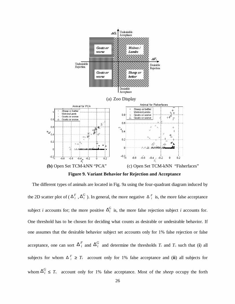
(a) Zoo Display

(b) Open Set TCM-kNN “PCA” (c) Open Set TCM-kNN “Fisherfaces”

Figure 9. Variant Behavior for Rejection and Acceptance

The different types of animals are located in Fig. 9a using the four-quadrant diagram induced by

the 2D scatter plot of ( Fi∆ ,

Gi∆ ). In general, the more negative Fi∆ is, the more false acceptance

subject i accounts for; the more positive Gi∆ is, the more false rejection subject i accounts for.

One threshold has to be chosen for deciding what counts as desirable or undesirable behavior. If

one assumes that the desirable behavior subject set accounts only for 1% false rejection or false

acceptance, one can sort Fi∆ and

Gi∆ and determine the thresholds TF and TG such that (i) all

subjects for whom Fi∆ ≥ TF account only for 1% false acceptance and (ii ) all subjects for

whomGi∆ ≤ TG account only for 1% false acceptance. Most of the sheep occupy the forth

27

quadrant and are characterized by desirable rejection behavior when Fi∆ is greater than TF and

desirable acceptance behavior when Gi∆ is less than TG. Note that if the PSR value of the probe is

far away from the threshold, the decisions are easy to make; only the parts of the distributions

near thresholds are likely to contribute to errors and need to be considered. The first quadrant is

characteristic of subjects that display desirable rejection behavior (when they should be indeed

rejected) but also of subjects showing undesirable rejection behavior (when they should be

accepted) (wolves / lambs). The second quadrant includes subjects that are difficult to label in

terms of rejection or recognition (goats). The third quadrant is characteristic of subjects that

display desirable acceptance behavior (when they should be accepted) but also of subjects

showing undesirable acceptance behavior when they should be instead rejected (goats). Finally,

the fourth quadrant represents subjects with good performance (sheep).

Open Set TCM - kNN using either PCA or Fisherfaces components is run 1,000 times to yield

the corresponding PSR scores. The overlap, of size m = 40, between the gallery and test sets of

size 80, is randomly chosen. The 2D scatter plots (for 150 subjects) of ( Fi∆ , G

i∆ ) for Open Set

TCM-kNN using PCA and Fisherfaces, respectively, are shown in Figs. 9b and 9c, respectively.

Most of the subjects show a central (near origin) tendency with good performance. Several

subjects show the tendency to deviate along one of the axis. Only few subjects show undesirable

characteristics along both axes. The average false rejection and false acceptance rates for Open

Set TCM - kNN using PCA components are 13.36% and 8.29%, respectively. The subjects with

the top 10 (20) Gi∆ values contribute 24.76% (50.09%) of total false rejection. The subjects with

top 10 (20) Fi∆− values contribute 28.54% (49.85%) of total false acceptance. The average false

rejection and false acceptance rates for Open Set TCM - kNN using Fisherfaces are 8.33% and

4.37%, respectively. The subjects with top 10 (20) Gi∆ values contribute 32.19% (62.64%) of

28

total false rejection. The subjects with top 10 (20) Fi∆− values contribute 38.74% (68.83%) of

total false acceptance.

The decision threshold is determined based on the above discussion for both PCA and

Fisherfaces components. For PCA, there are 52 (34.67%) subjects classified as Sheep or better,

28 (18.67%) as Wolves/Lambs, and 54 (36%) as Goats or worse in the third quadrant. Only 16

(10.67%) subjects are classified as Goats or worse in the second quadrant, and they contribute to

both 22.92% false rejection and 20.94% false acceptance. 37% of subjects are error prone animals

(not sheep) and they contribute about 98.2% and 98.9% of the total false rejection and false

acceptance errors, respectively. For Fisherfaces, there are 78 (52%) subjects classified as Sheep

or better, 24 (16%) as Wolves/Lambs, and 35 (23.3%) as Goats or worse in the third quadrant.

Only 13 (8.67%) subjects are classified as Goats or worse in the second quadrant, and they

contribute to both 32.1% false rejection and 29.0% false acceptance. 48% of subjects are error

prone animals (not sheep), and they contribute about 98.9% and 98.5% of total false rejection and

false acceptance errors, respectively. All the error prone animals contribute to either false

rejection or false acceptance for both PCA and Fisherfaces components. If some error prone

animals are removed from the test set, the performance for Open Set TCM-kNN will improve. As

an example, if all Goats or worse in the second quadrant are removed for PCA and Fisherfaces,

and the experiments in Sect. 7 are redone, the Open Set TCM-kNN performance improves and it

now achieves 85.69% and 91.63 % accuracy (at FAR = 3%) for PCA and Fisherfaces,

respectively, vs. the earlier results of 81% and 88% accuracy (at FAR = 6%).

10. Data Fusion

The overlap in labeling between Open Set TCM-kNN {PCA and Fisherfaces} regarding error

prone animals discussed in the previous section reveals useful insights about their comparative

29

contributions and suggests the possibility to fuse their outputs for enhanced authentication. Note

that data fusion for the outputs of different face recognition engines is a particular case of

information fusion (Ross and Jain, 2004) for multi(modal)-biometric systems (Jain and Ross,

2004) where different modalities, e.g., fingerprints, face and hand geometry, are used.

Multimodal biometrics that combine face and fingerprints have been shown to yield significant

performance improvement over single-mode biometric systems (Snelick et al., 2003). We

describe next how multi-system fusion using Open Set TCM-kNN {PCA and Fisherfaces} driven

by PSEI analysis yields better performance for authenticating those subjects that are rejected by

one classifier and accepted by another classifier.

Assume that during Open Set TCM-kNN the thresholds Θ, the training PSR standard

deviations, the probe PSR values and confidences for PCA and Fisherfaces are Θ PCA and Θ Fisher,

Stdev PCA and Stdev Fisher, PSR PCA and PSR Fisher, C PCA and C Fisher, respectively. The first case

occurs when the probe is accepted if both PSR PCA ≥ Θ PCA and PSR Fisher ≥ Θ Fisher. The

identification of the probe is then determined as follows: (i) If Open Set TCM-kNN {PCA and

Fisherfaces} yield the same ID for their largest (credibility) p-values, then the decision taken is to

authenticate the ID no matter what the confidences are; and (ii ) If the Open Set TCM-kNN {PCA,

Fisherfaces} yield different ID for their largest p-values, then choose that ID that yields larger

confidence. In the case when the two confidences are very close to each other, choose the label

coming from Open Set TCM-kNN Fisherfaces classifier because it yields better performance than

Open Set TCM-kNN PCA classifier (see Sect. 7).

The second case occurs when the probe is rejected if both PSR PCA < Θ PCA and PSR Fisher < Θ

Fisher. The third possible case occurs when PSR PCA ≥ Θ PCA and PSR Fisher < Θ Fisher, i.e., the two

engines disagree if rejection should take place. One has now to consider how far the probe PSRs

30

are away from the thresholds Θ and the relative location of the class predicted by Open Set TCM-

KNN PCA in the zoo. When the label predicted by Open Set TCM-KNN PCA is a sheep, the

probe is accepted and its ID is that predicted. If the label predicted by Open Set TCM-kNN PCA

is not a sheep then compare the following distances α = (PSR PCA - Θ PCA) / Stdev PCA and β= (Θ

Fisher - PSR Fisher )/ Stdev Fisher. If min (α,β) < T0 =2, i.e., two additional standard deviations, then if α

> β the ID that Open Set TCM-kNN PCA predicts is accepted; otherwise the probe is rejected. If

min (α,β) > T0, the probe is rejected using the very decision Open Set TCM-kNN Fisherfaces

classifier makes. Similar arguments apply for the last case when PSR PCA < Θ PCA and PSR Fisher ≥

Θ Fisher. Using the data fusion procedure described above, the experiments in Sect. 7 were redone

to yield now 91.55% accuracy and only 3.1% false alarm vs. 81% and 88% correct accuracy and

false alarm of 6% without fusion. Note that one achieves 91% accuracy without excluding any

error prone exemplar (see Sect. 9). Note that PCA and Fisherfaces are not independent

representations. Some animals were observed to continue to be error prone after the LDA step (of

Fisherfaces) once they were bad for PCA. In our data set, only 33 subjects are sheep for both

PCA and Fisherfaces components, while 64 subjects are sheep for either PCA or Fisherfaces

components.

11. Conclusions

This paper expands on the Transduction Confidence Machine (Proedrou, 2001) to make it

suitable for the open set recognition problem. Towards that end we introduced the Open Set

TCM – kNN (Transduction Confidence Machine – k Nearest Neighbors), a novel realization of

transductive inference that is suitable for open set multi-class classification and includes a

rejection option. Extensive experimental data, using challenging FERET data, shows the

comparative advantages of Open Set TCM-kNN. The major contributions made include multi-

31

class transductive inference using a priori threshold setting, effective open set identification and

watch list, meaningful error analysis to determine the uneven contributions to errors made by

different face patterns and their use for effective data fusion.

The proposed rejection functionality for open set recognition is similar to that used in

detection theory, hypothesis testing, and score normalization (See Sect. 5). The availability of the

rejection option, i.e., “none of the above” answer, in open set recognition, is similar to outlier

detection (in clustering) and novelty detection, topics of further investigation. The comparative

advantages of our proposed method come from its non-parametric implementation and automatic

threshold selection. No assumptions are made regarding the underlying probability density

functions responsible for the observed data clusters, i.e., the face IDs. Learning and training,

driven by transduction, are local. They provide robust information to detect outlier faces, i.e.,

unknown faces, and to reject them accordingly. Outlier detection corresponds to change

detection when faces or patterns change their appearance. Feature selection for enhanced pattern

recognition can be further achieved using strangeness and the p-value function. The stranger the

feature values are the better the discrimination between the patterns.

The acquisition and/or generation of additional exemplars for each class (to increase k in Open

Set TCM-kNN) is presently under investigation and is expected to lead to improved performance.

Another direction for future research concerns taking advantage of the linkage between

transductive inference (see Sects. 3 – 5), active learning, co-training, and normalization methods.

The active learner has to decide whether or not to request labels (“classification”) for unlabeled

data in order to reduce the volume of computation and the human effort involved in labeling

(Tong and Keller, 2001). Active learning selects, one by one, the most informative patterns from

some working set W, such that, after labeling by an expert (“classifier”), they will guarantee the

best improvement in the classifier performance. As an example, the sampling strategy proposed by

32

Juszczak and Duin (2004) relies on measuring the variation in label assignments (of the unlabeled

set) between the classifier trained on T and the classifier trained on T with a single unlabeled

exemplar e labeled with all possible labels. The use of unlabeled data, independent of the learning

algorithm, is characteristic of co–training (Blum and Mitchell, 1998; Nigam et al., 2000). The

idea of co–training is to learn two classifiers which bootstrap each other using labels for the

unlabeled data (Krogel and Scheffer, 2004). Co–training leads to improved performance if at least

one classifier labels at least one unlabeled instance correctly for which the other classifier currently

errs. Unlabeled examples which are confidently labeled by one classifier are then added, with

labels, to the training set of the other classifier.

References

[1]. E. Bailly-Bailliere et al. (2003), The BANCA Database and Evaluation Protocol, 4th Audio-

Video Based Person Authentication (AVBPA), 625 – 638.

[2]. S. Bengio, J. Mariethoz, and S. Marcel (2001), Evaluation of Biometric Technology on

XM2VTS, IDIAP-RR 01-21, European Project BANCA Deliverable D71, Martigny,

Switzerland.

[3]. A. Blum and T. Mitchell (1998), Combining Labeled and Unlabeled Data with Co-Training, in

COLT: Proc. of the Conf. on Computational Learning Theory, 92 – 100, Morgan Kaufmann.

[4]. R. M. Bolle, J. H. Connell, S. Pankanti, N. K. Ratha, and A. W. Senior (2004), Guide to

Biometrics, Springer.

[5]. R. Chellappa, C. L. Wilson and S. Sirohey (1995), Human and Machine Recognition of Faces:

A Survey, Proc. IEEE, Vol. 83, No. 5, 705 – 740.

[6]. T. M. Cover and P. E. Hart (1967), Nearest neighbor pattern classification, IEEE Trans.

Inform. Theory IT 13:21-7.

[7]. P. Grother (2004), Face Recognition Vendor Test 2002, Supplemental Report–NISTIR 7083.

33

[8]. J. Daugman (1997), Face and Gesture Recognition: Overview, IEEE Trans. on PAMI, Vol.

19, 7, 675 – 676.

[9]. G. R. Doddington, W. Liggett, A. Martin, M. Przybocki and D. Reynolds (1998), Sheep,

Goats, Lambs and Wolves: A Statistical Analysis of Speaker Performance, Proc. Of IC-

SLD’98, 1351-1354.

[10]. S. Furui (1997), Recent Advances in Speaker Recognition, Pattern Recognition Letters, 18,

859 – 872.

[11]. A. Gammerman, V. Vovk, and V. Vapnik (1998), Learning by Transduction. In Uncertainty

in Artificial Intelligence, 148 – 155.

[12]. A. Jain, R. Bolle, and S. Pankanti (Eds.) (1999), BIOMETRICS – Personal Identification in

Networked Society, Kluwer.

[13]. A. Jain and A. Ross (2004), Multibiometric Systems, Comm. of ACM, Vol.47, No.1,34– 40.

[14]. T. Joachims (1999), Transductive Inference for Text Classification Using Support Vector

Machines, in I. Bratko and S. Dzeroski (eds.), Proc. Of ICML-99, 16th Int. Conf. on

Machine Learning, Bled, Slovenia, Morgan Kaufmann, 200 - 209.

[15]. P. Juszczak and R. P. W. Duin (2004), Selective Sampling Based on the Variation in Label

Assignment, 17th Int. Conf. on Pattern Recognition (ICPR), Cambridge, England.

[16]. M. A. Krogel and T. Scheffer (2004), Multi-Relational Learning, Text Mining, and Semi-

Supervised Learning from Functional Genomics, Machine Learning, 57, 61 – 81.

[17]. M. Kukar and I. Kononenko (2002), Reliable Classifications with Machine Learning, 13th

European Conf. on Machine Learning (ECML), Helsinki, Finland.

[18]. M. Li and P. Vitanyi (1997), An Introduction to Kolmogorov Complexity and Its

Applications, 2nd. Springer-Verlag.

34

[19]. C. Liu and H. Wechsler (2002), Gabor Feature Based Classification Using the Enhanced

Fisher Linear Discriminant Model for Face Recognition, IEEE Trans. on Image Processing,

Vol. 11, No. 4, 467 – 476.

[20]. C. Liu and H. Wechsler (2004), Facial Recognition in Biometric Authentication:

Technologies, Systems, Evaluations and Legal Issues, J.L.Wayman, A. Jain, D. Maltoni and

D. Maio (Eds.), Springer-Verlag (to appear).

[21]. M.W. Mak, W.D. Zhang and M.X. He (2001), A New Two-Stage Scoring Normalization

Approach to Speaker Verification," Proc. Int. Sym. on Intelligent Multimedia, Video and

Speech Processing, pp. 107-110, Hong Kong.

[22]. T. Melluish, C. Suanders, I. Nouretdinov, I and V. Vovk (2001), The Typicalness

Framework: A Comparison with the Bayesian Approach. TR, Dept. of Computer Science,

Royal Holloway, University of London, http://www.clrc.rhul.ac.uk/tech-report/.

[23]. T. Mitchell (1999), The Role of Unlabelled Data in Supervised Learning, Proc. 6th Int.

Colloquium on Cognitive Sciences, San Sebastian, Spain.

[24]. K. Nigam, A. K. McCallum, S. Thrun and T. M. Mitchell (2000), Text Classification from

Labeled and Unlabeled Documents Using EM, Machine Learning, 39 (2/3), 103 – 134.

[25]. S. Pankanti, N. K. Ratha and R. M. Bolle (2002), Structure in Errors: A Case Study in

Fingerprint Verification, 16th Int. Conf. on Pattern Recognition, Quebec-City, Canada.

[26]. P. J. Phillips, H. Wechsler, J. Huang, and P. Rauss (1998), The FERET Database and

Evaluation Procedure for Face Recognition Algorithms, Image and Vision Computing, Vol.

16, No. 5, 295- 306.

[27]. P. J. Phillips, P. Grother, R. J. Micheals, D. M. Blackburn, E. Tabassi and M. Bone (2003),

Face Recognition Vendor Test 2002 – Overview and Summary.

35

[28]. K. Proedrou, I. Nouretdinov, V. Vovk and A. Gammerman (2001), Transductive

Confidence Machines for Pattern Recognition, TR CLRC-TR-01-02, Royal Holloway

University of London.

[29]. D. A. Reynolds, T. F. Quatieri, and R. B. Dunn (2000), Speaker Verification Using Adapted

Gaussian Mixture Models, Digital Signal Processing 10, 19 – 41.

[30]. A. Ross and A. Jain (2004), Information fusion in Biometrics, Pattern Recognition Letters,

Vol. 24, 2115 – 2125.

[31]. C. Saunders, A. Gammerman, and V. Vovk (1999), Transduction with Confidence and

Credibility, 16th Int. Joint Conf. on Artificial Intelligence (IJCAI), Stockholm, Sweden.

[32]. R. Snelick, M. Indovina, J. Yen, and A. Mink (2003), Multimodal Biometrics: Issues in

Design and Testing, ICMI’03, Vancouver, BC, Canada.

[33]. S. Tong and D. Koller (2001), Support Vector Machines Active Learning with Applications

to Text Classification, Journal of Machine Learning Research, Vol. 2, 45 – 66

[34]. V. N. Vapnik (1998), Statistical Learning Theory, Wiley.

[35]. V.N. Vapnik (2000), The Nature of Statistical Learning Theory, 2nd. Ed., Springer–Verlag.

[36]. W.J.Conover, Practical Nonparametric Statistics, John Wiley & Sons, Inc. 1980.

[37]. V. Vovk, A. Gammerman and C. Saunders (1999), Machine-Learning Application of

Algorithmic Randomness, Proceedings of the1 6th International Conference on Machine

Learning, Bled, Slovenia.

[38]. W. Zhao, R. Chellappa, P. J. Phillips, and A. Rosenfeld (2003), Face Recognition: A

Literature Survey, Computing Surveys, Vol. 35, No. 4, 399 – 458.