Open Source GIS Tutorial 11: Produce a carbon dataset

STEP-BY-STEP TUTORIAL V1.0:

ADDING BELOW-GROUND BIOMASS TO A DATASET

OF ABOVE-GROUND BIOMASS AND CONVERTING TO

CARBON USING QGIS 1.8

USING SPATIAL INFORMATION TO SUPPORT DECISIONS ON

SAFEGUARDS AND MULTIPLE BENEFITS FOR REDD+

Using open source GIS software to support REDD+ planning

The UN-REDD Programme is the United Nations Collaborative initiative on Reducing Emissions from

Deforestation and forest Degradation (REDD) in developing countries. The Programme was launched in

September 2008 to assist developing countries prepare and implement national REDD+ strategies, and

builds on the convening power and expertise of the Food and Agriculture Organization of the United

Nations (FAO), the United Nations Development Programme (UNDP) and the United Nations Environment

Programme (UNEP).

The United Nations Environment Programme World Conservation Monitoring Centre (UNEP-WCMC) is the

specialist biodiversity assessment centre of the United Nations Environment Programme (UNEP), the

world’s foremost intergovernmental environmental organisation. The Centre has been in operation for

over 30 years, combining scientific research with practical policy advice.

Prepared by Corinna Ravilious, Andy Arnell and Blaise Bodin

Copyright: UNEP

Copyright release: This publication may be reproduced for educational or non-profit purposes without

special permission, provided acknowledgement to the source is made. Re-use of any figures is subject to

permission from the original rights holders. No use of this publication may be made for resale or any other

commercial purpose without permission in writing from UNEP. Applications for permission, with a

statement of purpose and extent of reproduction, should be sent to the Director, UNEP-WCMC, 219

Huntingdon Road, Cambridge, CB3 0DL, UK.

Disclaimer: The contents of this report do not necessarily reflect the views or policies of UNEP,

contributory organisations or editors. The designations employed and the presentations of material in this

report do not imply the expression of any opinion whatsoever on the part of UNEP or contributory

organisations, editors or publishers concerning the legal status of any country, territory, city area or its

authorities, or concerning the delimitation of its frontiers or boundaries or the designation of its name,

frontiers or boundaries. The mention of a commercial entity or product in this publication does not imply

endorsement by UNEP.

We welcome comments on any errors or issues. Should readers wish to comment on this document, they

are encouraged to get in touch via: [email protected].

Citation: Ravilious, C., Arnell, A. and Bodin, B. (2015) Using spatial information to support decisions on

safeguards and multiple benefits for REDD+. Step-by-step tutorial v1.0: Adding below-ground biomass to a

dataset of above-ground biomass and converting to carbon using QGIS 1.8. Prepared on behalf of the UN-

REDD Programme. UNEP World Conservation Monitoring Centre, Cambridge, UK.

Acknowledgements: These training materials have been produced from materials generated for

working sessions held in various countries to aid the production of multiple benefits maps to inform

REDD+ planning and safeguards policies using open source GIS software.

mailto:[email protected]


Contents

1. Introduction .................................................................................................................... 1

2. Produce a carbon dataset which includes above and below-ground biomass .................... 1

2.1 Project ecological zones and above-ground biomass to same projection ........................... 1

2.2 Convert ecological zones from vector to raster .................................................................... 3

2.3 Calculate below-ground biomass according to IPCC values and convert to carbon............. 5


1

1. Introduction

REDD+ has the potential to deliver multiple benefits beyond carbon. For example, it can promote

biodiversity conservation and secure ecosystem services from forests such as water regulation,

erosion control and non-timber forest products. Some of the potential benefits from REDD+, such as

biodiversity conservation, can be enhanced through identifying areas where REDD+ actions might

have the greatest impact using spatial analysis.

Open Source GIS software can be used to undertake spatial analysis of datasets of relevance to

multiple benefits and environmental safeguards for REDD+. Open-source software is released under a

license that allows software to be freely used, modified, and shared (http://opensource.org/licenses).

Therefore, using open source software has great potential in building sustainable capacity and critical

mass of experts with limited financial resources.

2. Produce a carbon dataset which includes above and below-ground

biomass 2.1 Project ecological zones and above-ground biomass to same projection

The aim is to produce a raster dataset combining both above and below-ground biomass and to

convert these values to carbon. Below-ground biomass is generated by applying IPCC conversion

factors to the above-ground biomass to calculate a below-ground proportion. The conversion factors

are applied depending upon ecological zone (e.g. in this example from the FAO ecological zones

dataset).

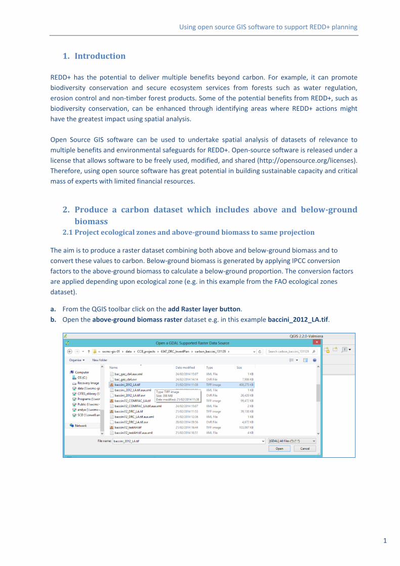
a. From the QGIS toolbar click on the add Raster layer button.

b. Open the above-ground biomass raster dataset e.g. in this example baccini_2012_LA.tif.


2

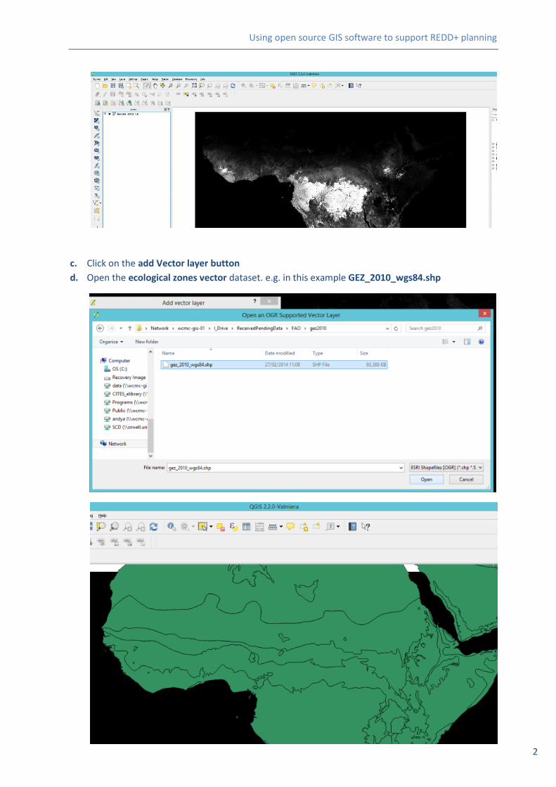
c. Click on the add Vector layer button

d. Open the ecological zones vector dataset. e.g. in this example GEZ_2010_wgs84.shp


3

e. Check the coordinate systems of the two layers. The vector layer is likely to be in wgs84 and the

above-ground biomass raster layer may be in another projection e.g. in this example in Lambert

Azimuthal Equal area projection, which may be shown as a user defined coordinate system.

In this case the ecological zones dataset is in WGS84 and needs to be converted to the same

projection system as the above-ground biomass dataset.

Sometimes, errors can be encountered when using the Reproject tool for this step in QGIS, hence the

following approach of saving the shapefile as a new layer to project it into the correct system should

be used.

f. Right click on the ecological zones layer and click Save as

g. Browse to and choose an output directory and name for the shapefile output.

h. Under the CRS heading, browse to and select the same coordinate system as the above-ground

biomass dataset.

i. Open the newly created dataset. Right click in properties and check that the CRS is the same as

the above-ground biomass dataset.

j. It is useful to ensure consistent CRS for outputs by making sure the project reference system for

the project is consistent with these layers: right click on the above-ground biomass raster layer,

and select set project CRS from layer.

2.2 Convert ecological zones from vector to raster

a. View and check the attribute table from the

ecological zones vector dataset – making sure

individual codes (in the gez_code column) are

present. These values relate to the names of the

ecological zones (in the gez_name column) and

will be chosen to be transferred to become

raster values when converting from a vector to a

raster layer in the next step.

b. Make sure the processing toolbox is open – it

should appear in the right hand side of the

screen. If it is not active then click on the

processing>>toolbox to activate it.

c. Convert the file to raster using the rasterize tool within

the processing toolbox (also referred to as the shapes

to grid tool). Search for shapes in the toolbox

d. Double click on the Shapes to grid tool


4

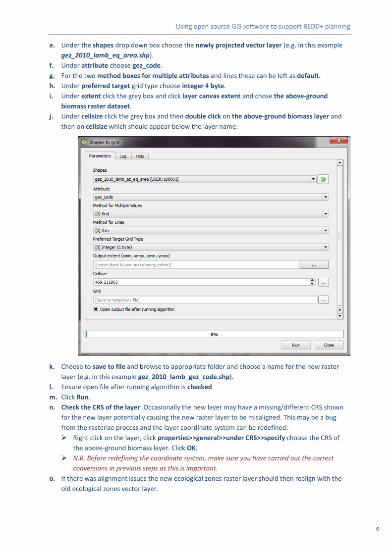
e. Under the shapes drop down box choose the newly projected vector layer (e.g. in this example

gez_2010_lamb_eq_area.shp).

f. Under attribute choose gez_code.

g. For the two method boxes for multiple attributes and lines these can be left as default.

h. Under preferred target grid type choose integer 4 byte.

i. Under extent click the grey box and click layer canvas extent and chose the above-ground

biomass raster dataset.

j. Under cellsize click the grey box and then double click on the above-ground biomass layer and

then on cellsize which should appear below the layer name.

k. Choose to save to file and browse to appropriate folder and choose a name for the new raster

layer (e.g. in this example gez_2010_lamb_gez_code.shp).

l. Ensure open file after running algorithm is checked

m. Click Run.

n. Check the CRS of the layer. Occasionally the new layer may have a missing/different CRS shown

for the new layer potentially causing the new raster layer to be misaligned. This may be a bug

from the rasterize process and the layer coordinate system can be redefined:

Right click on the layer, click properties>>general>>under CRS>>specify choose the CRS of

the above-ground biomass layer. Click OK.

N.B. Before redefining the coordinate system, make sure you have carried out the correct

conversions in previous steps as this is important.

o. If there was alignment issues the new ecological zones raster layer should then realign with the

old ecological zones vector layer.


5

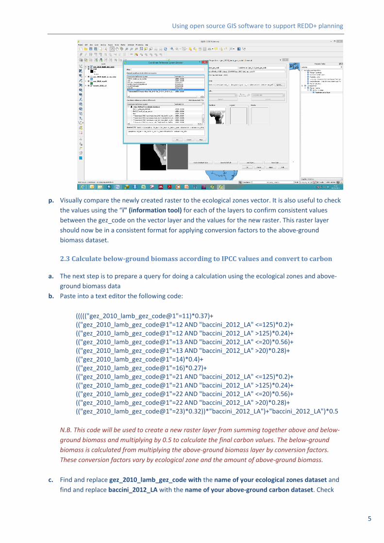
p. Visually compare the newly created raster to the ecological zones vector. It is also useful to check

the values using the “i" (information tool) for each of the layers to confirm consistent values

between the gez_code on the vector layer and the values for the new raster. This raster layer

should now be in a consistent format for applying conversion factors to the above-ground

biomass dataset.

2.3 Calculate below-ground biomass according to IPCC values and convert to carbon

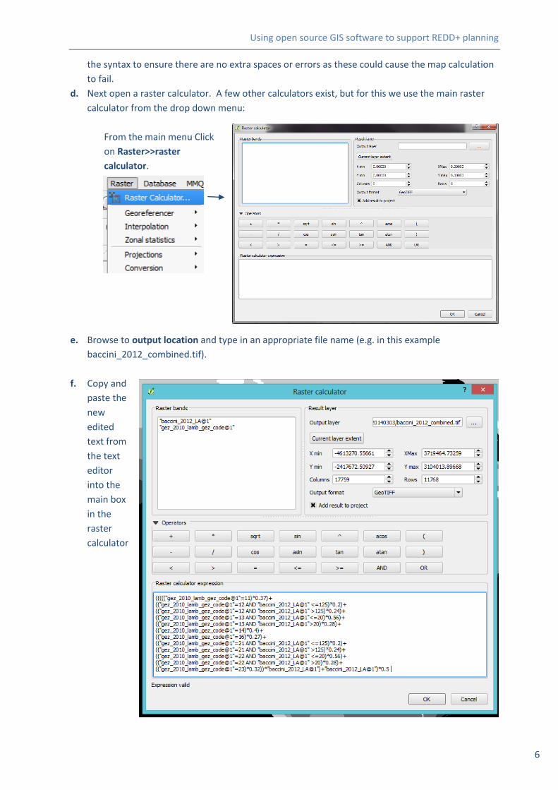
a. The next step is to prepare a query for doing a calculation using the ecological zones and above-

ground biomass data

b. Paste into a text editor the following code:

((((("gez_2010_lamb_gez_code@1"=11)*0.37)+ (("gez_2010_lamb_gez_code@1"=12 AND "baccini_2012_LA" <=125)*0.2)+ (("gez_2010_lamb_gez_code@1"=12 AND "baccini_2012_LA" >125)*0.24)+ (("gez_2010_lamb_gez_code@1"=13 AND "baccini_2012_LA" <=20)*0.56)+ (("gez_2010_lamb_gez_code@1"=13 AND "baccini_2012_LA" >20)*0.28)+ (("gez_2010_lamb_gez_code@1"=14)*0.4)+ (("gez_2010_lamb_gez_code@1"=16)*0.27)+ (("gez_2010_lamb_gez_code@1"=21 AND "baccini_2012_LA" <=125)*0.2)+ (("gez_2010_lamb_gez_code@1"=21 AND "baccini_2012_LA" >125)*0.24)+ (("gez_2010_lamb_gez_code@1"=22 AND "baccini_2012_LA" <=20)*0.56)+ (("gez_2010_lamb_gez_code@1"=22 AND "baccini_2012_LA" >20)*0.28)+ (("gez_2010_lamb_gez_code@1"=23)*0.32))*"baccini_2012_LA")+"baccini_2012_LA")*0.5

N.B. This code will be used to create a new raster layer from summing together above and below-

ground biomass and multiplying by 0.5 to calculate the final carbon values. The below-ground

biomass is calculated from multiplying the above-ground biomass layer by conversion factors.

These conversion factors vary by ecological zone and the amount of above-ground biomass.

c. Find and replace gez_2010_lamb_gez_code with the name of your ecological zones dataset and

find and replace baccini_2012_LA with the name of your above-ground carbon dataset. Check


6

the syntax to ensure there are no extra spaces or errors as these could cause the map calculation

to fail.

d. Next open a raster calculator. A few other calculators exist, but for this we use the main raster

calculator from the drop down menu:

From the main menu Click

on Raster>>raster

calculator.

e. Browse to output location and type in an appropriate file name (e.g. in this example

baccini_2012_combined.tif).

f. Copy and

paste the

new

edited

text from

the text

editor

into the

main box

in the

raster

calculator


7

g. After the code is pasted in the main box, the message at the bottom should change from

“Expression invalid” to “Expression valid”.

h. Navigate to an output folder and give it a new name e.g. in this example baccini_2012

_combined.

i. Click OK to perform the calculation. The processing progress bar should come up and the resulting

output layer should appear in the table of contents.

N.B. When using the raster calculator, be careful to make sure there are no misspell names for layers

or other similar errors in the code. From experience it seems the calculator may allow an expression to

run and appear valid, even when errors exist such as incorrect file names, resulting in an output raster

of Null and Zero values.

j. Check the final layer produced makes sense, using the “i” (information tool) to check that some

of the values make sense, considering the magnitude of the conversion factors and the original

datasets used to derive the final output.

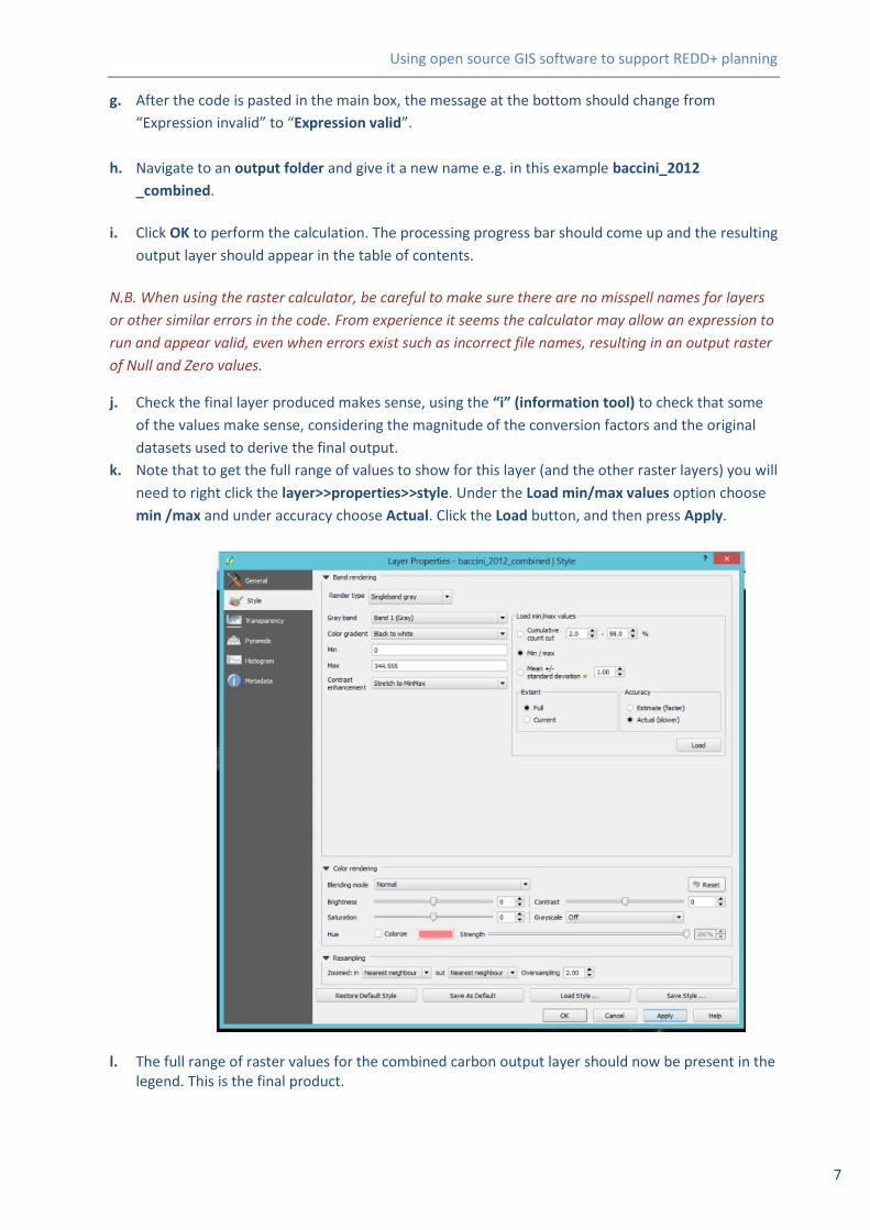
k. Note that to get the full range of values to show for this layer (and the other raster layers) you will

need to right click the layer>>properties>>style. Under the Load min/max values option choose

min /max and under accuracy choose Actual. Click the Load button, and then press Apply.

l. The full range of raster values for the combined carbon output layer should now be present in the legend. This is the final product.

Documents

Open Source GIS Tutorial 11: Produce a carbon dataset