Operating cycle representations for road vehicles

THESIS FOR THE DEGREE OF DOCTOR OF PHILOSOPHY IN MACHINE ANDVEHICLE SYSTEMS

Operating cycle representations for road vehicles

PAR PETTERSSON

Department of Mechanics and Maritime SciencesCHALMERS UNIVERSITY OF TECHNOLOGY

Goteborg, Sweden 2019

Operating cycle representations for road vehiclesPAR PETTERSSONISBN 978-91-7905-210-2

c© PAR PETTERSSON, 2019

Doktorsavhandlingar vid Chalmers tekniska hogskolaNy serie nr. 4677ISSN 0346-718XDepartment of Mechanics and Maritime SciencesChalmers University of TechnologySE-412 96 GoteborgSwedenTelephone: +46 (0)31-772 1000

Cover:A polar bear in a snow storm.

Chalmers ReproserviceGoteborg, Sweden 2019

Operating cycle representations for road vehiclesPAR PETTERSSONDepartment of Mechanics and Maritime SciencesChalmers University of Technology

Abstract

This thesis discusses different ways to represent road transport operations mathematically.The intention is to make more realistic predictions of longitudinal performance measures forroad vehicles, such as the CO2 emissions. It is argued that a driver and vehicle independentdescription of relevant transport operations increase the chance that a predicted measurelater coincides with the actual measure from the vehicle in its real-world application. Thisallows for fair comparisons between vehicle designs and, by extension, effective productdevelopment.

Three different levels of representation are introduced, each with its own purpose andapplication.

The first representation, called the bird’s eye view, is a broad, high-level descriptionwith few details. It can be used to give a rough picture of the collection of all transportoperations that a vehicle executes during its lifetime. It is primarily useful as a classificationsystem to compare different applications and assess their similarity.

The second representation, called the stochastic operating cycle (sOC) format, is astatistical, mid-level description with a moderate amount of detail. It can be used togive a comprehensive statistical picture of transport operations, either individually oras a collection. It is primarily useful to measure and reproduce variation in operatingconditions, as it describes the physical properties of the road as stochastic processessubject to a hierarchical structure.

The third representation, called the deterministic operating cycle (dOC) format, isa physical, low-level description with a great amount of detail. It describes individualoperations and contains information about the road, the weather, the traffic and themission. It is primarily useful as input to dynamic simulations of longitudinal vehicledynamics.

Furthermore, it is discussed how to build a modular, dynamic simulation model thatcan use data from the dOC format to predict energy usage. At the top level, the completemodel has individual modules for the operating cycle, the driver and the vehicle. Theseshare information only through the same interfaces as in reality but have no componentsin common otherwise and can therefore be modelled separately. Implementations arebriefly presented for each module, after which the complete model is showcased in anumerical example.

The thesis ends with a discussion, some conclusions, and an outlook on possible waysto continue.

Keywords: operating cycle, transport operation description, road format, energy usage,CO2 emissions, full vehicle simulation

i

ii

I don’t like it and I’m sorry I ever had anything to do with it.Erwin Schrodinger, about his wave formulation of quantum mechanics upon realising itdid not make the (microscopic) world predictable and deterministic: it still had to be

interpreted through probabilities.

Acknowledgements

First, I would like to thank my main supervisor, Professor Bengt Jacobson, for thediscussions, the help and, especially, the support throughout these five years. My secondthanks go to my co-supervisors: Dr Fredrik Bruzelius, Dr Sixten Berglund and AndersEriksson. I would also like to thank the Swedish energy agency, Vinnova and FFI for thefinancial support.

I owe large chunks of gratitude to my main collaborators, Dr Par Johannesson and DrLars Fast at RISE. It has been a pleasure working with you, and I have learned a lot.

Next, I would like to thank Dr Jan Andersson and Bjorn Lindenberg at Volvo cars, DrFabio Santandrea and Francisco Diaz Pisano at RISE, Thierry Bondat, Tobias Axelsson,Hjalmar Sandberg, Henrik Ryberg and Stefan Edlund at Volvo trucks, and the membersof the OCEAN and COVER projects.

I would also like to thank past and present members at the VEAS department andthe vehicle dynamics group for providing an excellent working environment. Sonja, everthe champion of the PhD students, of course deserves a special mention, as does Dr Selpifor the support during the research studies. And to my PhD colleagues: thanks for thejoy and all the laughter! I have made friends for life. A special thanks to Tushar, Randiand Magnus, for the running, the climbing and, most of all, for making certain to dragme out of the office, all the times when I did not want to but needed it.

Finally, thank you mom, dad, Jon, Sivert and Benji. For everything.

iii

iv

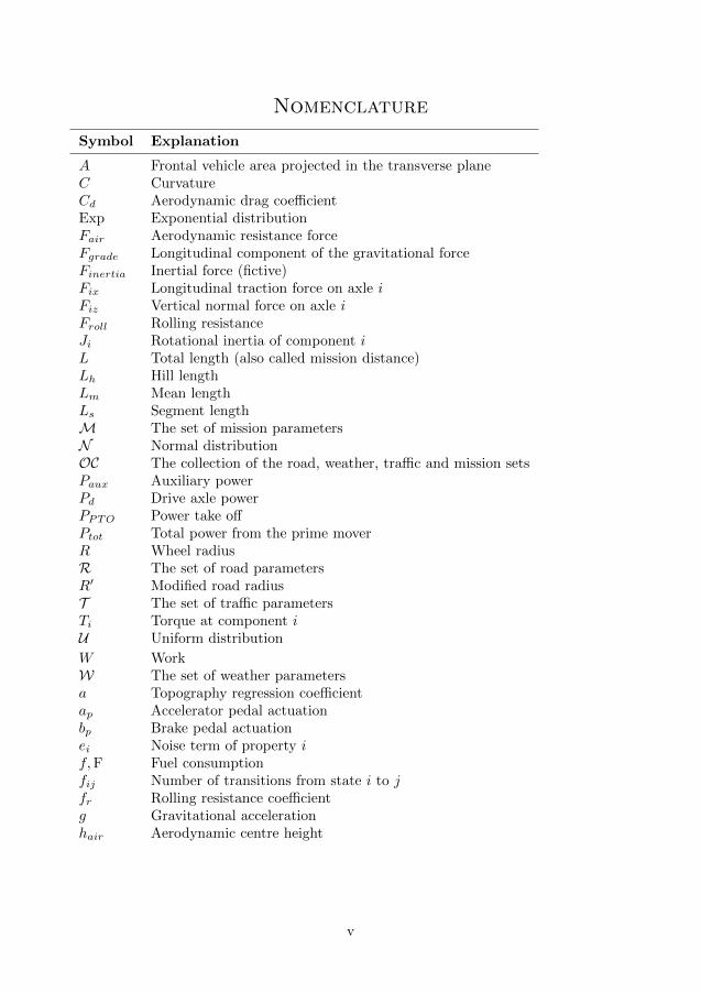
Nomenclature

Symbol Explanation

A Frontal vehicle area projected in the transverse planeC CurvatureCd Aerodynamic drag coefficientExp Exponential distributionFair Aerodynamic resistance forceFgrade Longitudinal component of the gravitational forceFinertia Inertial force (fictive)Fix Longitudinal traction force on axle iFiz Vertical normal force on axle iFroll Rolling resistanceJi Rotational inertia of component iL Total length (also called mission distance)Lh Hill lengthLm Mean lengthLs Segment lengthM The set of mission parametersN Normal distributionOC The collection of the road, weather, traffic and mission setsPaux Auxiliary powerPd Drive axle powerPPTO Power take offPtot Total power from the prime moverR Wheel radiusR The set of road parametersR′ Modified road radiusT The set of traffic parametersTi Torque at component iU Uniform distribution

W WorkW The set of weather parametersa Topography regression coefficientap Accelerator pedal actuationbp Brake pedal actuationei Noise term of property if,F Fuel consumptionfij Number of transitions from state i to jfr Rolling resistance coefficientg Gravitational accelerationhair Aerodynamic centre height

v

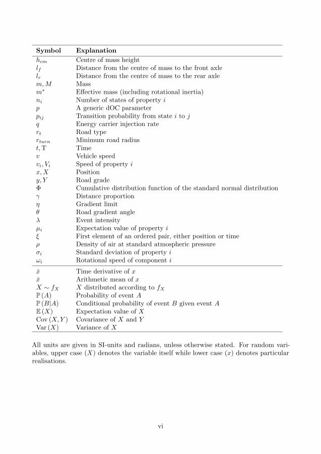
Symbol Explanation

hcm Centre of mass heightlf Distance from the centre of mass to the front axlelr Distance from the centre of mass to the rear axlem,M Massm∗ Effective mass (including rotational inertia)ni Number of states of property ip A generic dOC parameterpij Transition probability from state i to jq Energy carrier injection ratert Road typerturn Minimum road radiust,T Timev Vehicle speedvi, Vi Speed of property ix,X Positiony, Y Road gradeΦ Cumulative distribution function of the standard normal distributionγ Distance proportionη Gradient limitθ Road gradient angleλ Event intensityµi Expectation value of property iξ First element of an ordered pair, either position or timeρ Density of air at standard atmospheric pressureσi Standard deviation of property iωi Rotational speed of component i

x Time derivative of xx Arithmetic mean of xX ∼ fX X distributed according to fXP (A) Probability of event AP (B|A) Conditional probability of event B given event AE (X) Expectation value of XCov (X,Y ) Covariance of X and YVar (X) Variance of X

All units are given in SI-units and radians, unless otherwise stated. For random vari-ables, upper case (X) denotes the variable itself while lower case (x) denotes particularrealisations.

vi

Abbreviations

Abbreviation Explanation

dOC Deterministic operating cycleFBD Free body diagramGPS Global positioning systemGTA Global transport applicationLCV Long combination vehicleOC Operating cyclePTO Power take-offRAD Rear axle drive (axle configuration specifier)SD Standard deviationSE Standard errorsOC Stochastic operating cycleVECTO Vehicle energy consumption calculation toolWGS World geodetic systemWLTC World wide harmonised light duty test cyle

vii

viii

Thesis

This thesis consists of an extended summary and the following appended papers:

Paper A

P. Pettersson, S. Berglund, H. Ryberg, B. Jacobson, G. Karlsson, L.Brusved, and J. Bjernetun. Comparison of dual and single clutch trans-mission based on Global Transport Application mission profiles. Inter-national Journal of Vehicle Design 77.1/2 (Mar. 2019), pp. 22–42. doi:10.1504/IJVD.2018.098263

Paper B

P. Pettersson, S. Berglund, B. Jacobson, L. Fast, P. Johannesson, andF. Santandrea. A proposal for an operating cycle description format forroad transport missions. European Transport Research Review 10.31 (June2018), pp. 1–19. doi: 10.1186/s12544-018-0298-4

Paper C

P. Pettersson, P. Johannesson, B. Jacobson, F. Bruzelius, L. Fast, and S.Berglund. A statistical operating cycle description for prediction of roadvehicles’ energy consumption. Transportation Research Part D: Transportand Environment 73 (Aug. 2019), pp. 205–229. doi: 10.1016/j.trd.

2019.07.006

Paper DP. Pettersson, B. Jacobson, F. Bruzelius, P. Johannesson, and L. Fast.Intrinsic differences between backward and forward vehicle simulationmodels. Submitted to 21st IFAC world congress. Oct. 2019

In all papers, the author of the thesis wrote the vast majority of the text and wasresponsible for the modelling, simulation and data analysis.

Paper A was based on the engineering solution by Karlsson, Brusved, Bjernetun,Ryberg and others at Volvo trucks. Ryberg provided the experimental measurements andcontributed to the text together with Dr Berglund and Professor Jacobson. The ideasbehind the paper belong mostly to Dr Berglund. In Paper B, Dr Fast and Petterssoncarried out the experimental measurements. In Paper C, Dr Johannesson was the architectbehind the stochastic operating cycle format and wrote the generation software.

Other relevant publications by the author, but not included in the thesis:

I P. Pettersson, B. Jacobson, P. Johannesson, S. Berglund, and L. Laine. “Influenceof hill length on energy consumption for hybridized heavy transports in long haultransports”. 7th Commercial Vehicle Workshop Graz. Graz, Austria: TU Graz,May 2016. url: https://research.chalmers.se/publication/236668 (visitedon June 18, 2018)

II A. Odrigo, M. El-Gindy, P. Pettersson, Z. Nedelkova, P. Lindroth, and F. Oijer.Design and development of a road profile generator. International Journal ofVehicle Systems Modelling and Testing 11.3 (Dec. 2016), pp. 217–233. doi: 10.

1504/IJVSMT.2016.080875

ix

https://doi.org/10.1504/IJVD.2018.098263

https://doi.org/10.1186/s12544-018-0298-4

https://doi.org/10.1016/j.trd.2019.07.006


https://research.chalmers.se/publication/236668

https://doi.org/10.1504/IJVSMT.2016.080875


x

Contents

Abstract i

Acknowledgements iii

Nomenclature v

Abbreviations vii

Thesis ix

Contents xi

1 Introduction 11.1 Background . . . . . . . . . . . . . . . . . . . . . . . . . . . . . . . . . . . 1

1.1.1 The inadequacy of driving cycles . . . . . . . . . . . . . . . . . . . 51.1.2 The differences in application and the variation therein . . . . . . 7

1.2 Research questions . . . . . . . . . . . . . . . . . . . . . . . . . . . . . . . 91.3 Limitations . . . . . . . . . . . . . . . . . . . . . . . . . . . . . . . . . . . 101.4 Scientific contribution . . . . . . . . . . . . . . . . . . . . . . . . . . . . . 111.5 Thesis outline . . . . . . . . . . . . . . . . . . . . . . . . . . . . . . . . . . 11

2 Representing transport operations 132.1 What features need to be included? . . . . . . . . . . . . . . . . . . . . . . 132.2 A high-level description for classification . . . . . . . . . . . . . . . . . . . 16

2.2.1 The global transport application . . . . . . . . . . . . . . . . . . . 202.3 A mid-level description for variation . . . . . . . . . . . . . . . . . . . . . 23

2.3.1 Modelling individual road properties . . . . . . . . . . . . . . . . . 232.3.2 The stochastic operating cycle format . . . . . . . . . . . . . . . . 26

2.4 A low-level description for simulation . . . . . . . . . . . . . . . . . . . . . 292.4.1 The deterministic operating cycle format . . . . . . . . . . . . . . 30

2.5 Relations between representations . . . . . . . . . . . . . . . . . . . . . . 332.5.1 Stochastic model parameters as classification measures . . . . . . . 332.5.2 Generating transport operations from an sOC . . . . . . . . . . . . 36

3 Modelling and simulation 413.1 Model topology . . . . . . . . . . . . . . . . . . . . . . . . . . . . . . . . . 41

3.1.1 An operating cycle model . . . . . . . . . . . . . . . . . . . . . . . 423.1.2 A driver model . . . . . . . . . . . . . . . . . . . . . . . . . . . . . 443.1.3 A vehicle model . . . . . . . . . . . . . . . . . . . . . . . . . . . . 45

3.2 Predicting CO2 emissions through simulation . . . . . . . . . . . . . . . . 473.2.1 An example in goods distribution . . . . . . . . . . . . . . . . . . . 483.2.2 About expected consumption, variance and mission length . . . . . 51

xi

4 Discussion, conclusion and outlook 554.1 Discussion and conclusion . . . . . . . . . . . . . . . . . . . . . . . . . . . 554.2 Outlook . . . . . . . . . . . . . . . . . . . . . . . . . . . . . . . . . . . . . 58

References 61

Paper A 77

Paper B 97

Paper C 123

Paper D 157

xii

Extended Summary

1 Introduction

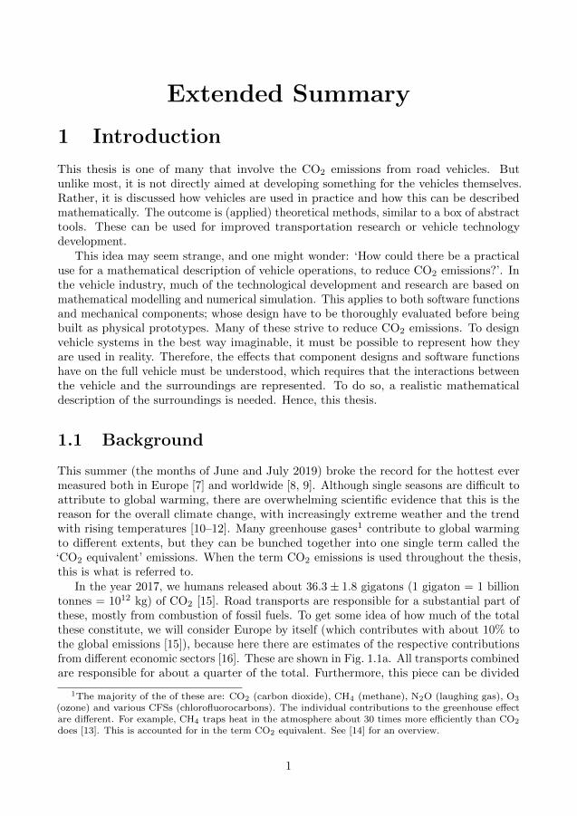
This thesis is one of many that involve the CO2 emissions from road vehicles. Butunlike most, it is not directly aimed at developing something for the vehicles themselves.Rather, it is discussed how vehicles are used in practice and how this can be describedmathematically. The outcome is (applied) theoretical methods, similar to a box of abstracttools. These can be used for improved transportation research or vehicle technologydevelopment.

This idea may seem strange, and one might wonder: ‘How could there be a practicaluse for a mathematical description of vehicle operations, to reduce CO2 emissions?’. Inthe vehicle industry, much of the technological development and research are based onmathematical modelling and numerical simulation. This applies to both software functionsand mechanical components; whose design have to be thoroughly evaluated before beingbuilt as physical prototypes. Many of these strive to reduce CO2 emissions. To designvehicle systems in the best way imaginable, it must be possible to represent how theyare used in reality. Therefore, the effects that component designs and software functionshave on the full vehicle must be understood, which requires that the interactions betweenthe vehicle and the surroundings are represented. To do so, a realistic mathematicaldescription of the surroundings is needed. Hence, this thesis.

1.1 Background

This summer (the months of June and July 2019) broke the record for the hottest evermeasured both in Europe [7] and worldwide [8, 9]. Although single seasons are difficult toattribute to global warming, there are overwhelming scientific evidence that this is thereason for the overall climate change, with increasingly extreme weather and the trendwith rising temperatures [10–12]. Many greenhouse gases1 contribute to global warmingto different extents, but they can be bunched together into one single term called the‘CO2 equivalent’ emissions. When the term CO2 emissions is used throughout the thesis,this is what is referred to.

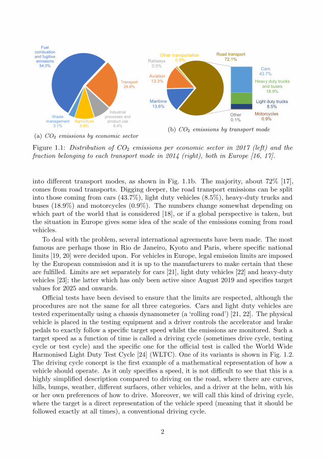
In the year 2017, we humans released about 36.3± 1.8 gigatons (1 gigaton = 1 billiontonnes = 1012 kg) of CO2 [15]. Road transports are responsible for a substantial part ofthese, mostly from combustion of fossil fuels. To get some idea of how much of the totalthese constitute, we will consider Europe by itself (which contributes with about 10% tothe global emissions [15]), because here there are estimates of the respective contributionsfrom different economic sectors [16]. These are shown in Fig. 1.1a. All transports combinedare responsible for about a quarter of the total. Furthermore, this piece can be divided

1The majority of the of these are: CO2 (carbon dioxide), CH4 (methane), N2O (laughing gas), O3

(ozone) and various CFSs (chlorofluorocarbons). The individual contributions to the greenhouse effectare different. For example, CH4 traps heat in the atmosphere about 30 times more efficiently than CO2

does [13]. This is accounted for in the term CO2 equivalent. See [14] for an overview.

1

Fuel combustion and fugitive emissions

54.0%

Transport24.6%

Industrial processes and

product use8.4%

Agriculture9.8%

Waste management

3.1%

(a) CO2 emissions by economic sector

Maritime13.6%

Aviation13.3%

Railways0.5%

Other transportation0.5%

Cars43.7%

Heavy duty trucks and buses

18.9%

Light duty trucks8.5%

Motorcycles0.9%

Other0.1%

Road transport72.1%

(b) CO2 emissions by transport mode

Figure 1.1: Distribution of CO2 emissions per economic sector in 2017 (left) and thefraction belonging to each transport mode in 2014 (right), both in Europe [16, 17].

into different transport modes, as shown in Fig. 1.1b. The majority, about 72% [17],comes from road transports. Digging deeper, the road transport emissions can be splitinto those coming from cars (43.7%), light duty vehicles (8.5%), heavy-duty trucks andbuses (18.9%) and motorcycles (0.9%). The numbers change somewhat depending onwhich part of the world that is considered [18], or if a global perspective is taken, butthe situation in Europe gives some idea of the scale of the emissions coming from roadvehicles.

To deal with the problem, several international agreements have been made. The mostfamous are perhaps those in Rio de Janeiro, Kyoto and Paris, where specific nationallimits [19, 20] were decided upon. For vehicles in Europe, legal emission limits are imposedby the European commission and it is up to the manufacturers to make certain that theseare fulfilled. Limits are set separately for cars [21], light duty vehicles [22] and heavy-dutyvehicles [23]; the latter which has only been active since August 2019 and specifies targetvalues for 2025 and onwards.

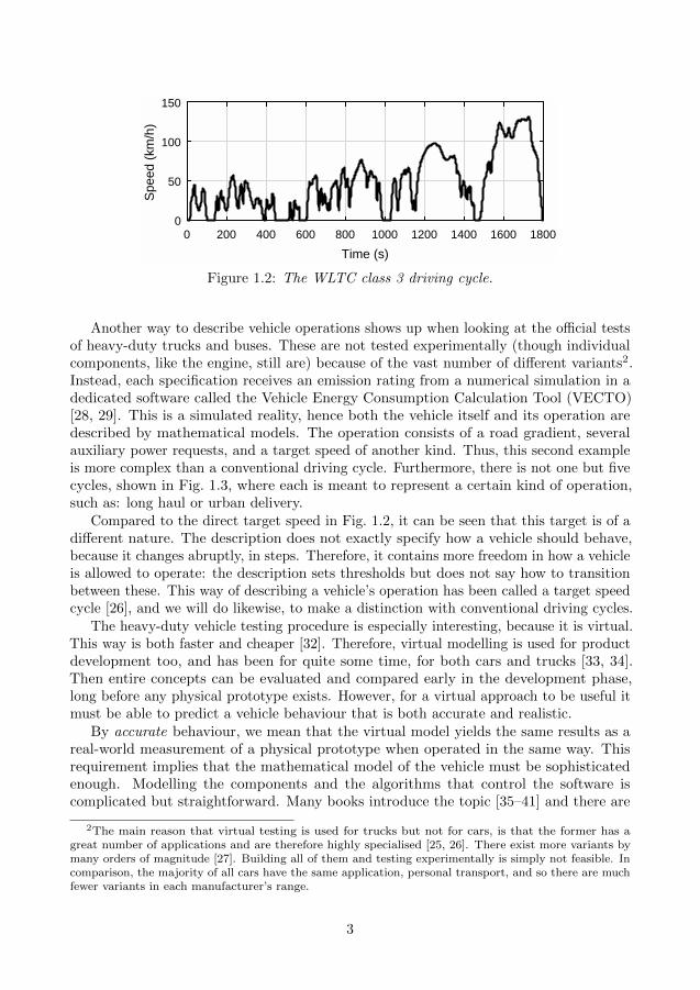
Official tests have been devised to ensure that the limits are respected, although theprocedures are not the same for all three categories. Cars and light duty vehicles aretested experimentally using a chassis dynamometer (a ‘rolling road’) [21, 22]. The physicalvehicle is placed in the testing equipment and a driver controls the accelerator and brakepedals to exactly follow a specific target speed whilst the emissions are monitored. Such atarget speed as a function of time is called a driving cycle (sometimes drive cycle, testingcycle or test cycle) and the specific one for the official test is called the World WideHarmonised Light Duty Test Cycle [24] (WLTC). One of its variants is shown in Fig. 1.2.The driving cycle concept is the first example of a mathematical representation of how avehicle should operate. As it only specifies a speed, it is not difficult to see that this is ahighly simplified description compared to driving on the road, where there are curves,hills, bumps, weather, different surfaces, other vehicles, and a driver at the helm, with hisor her own preferences of how to drive. Moreover, we will call this kind of driving cycle,where the target is a direct representation of the vehicle speed (meaning that it should befollowed exactly at all times), a conventional driving cycle.

2

0 200 400 600 800 1000 1200 1400 1600 1800

Time (s)

0

50

100

150

Spe

ed (

km/h

)

Figure 1.2: The WLTC class 3 driving cycle.

Another way to describe vehicle operations shows up when looking at the official testsof heavy-duty trucks and buses. These are not tested experimentally (though individualcomponents, like the engine, still are) because of the vast number of different variants2.Instead, each specification receives an emission rating from a numerical simulation in adedicated software called the Vehicle Energy Consumption Calculation Tool (VECTO)[28, 29]. This is a simulated reality, hence both the vehicle itself and its operation aredescribed by mathematical models. The operation consists of a road gradient, severalauxiliary power requests, and a target speed of another kind. Thus, this second exampleis more complex than a conventional driving cycle. Furthermore, there is not one but fivecycles, shown in Fig. 1.3, where each is meant to represent a certain kind of operation,such as: long haul or urban delivery.

Compared to the direct target speed in Fig. 1.2, it can be seen that this target is of adifferent nature. The description does not exactly specify how a vehicle should behave,because it changes abruptly, in steps. Therefore, it contains more freedom in how a vehicleis allowed to operate: the description sets thresholds but does not say how to transitionbetween these. This way of describing a vehicle’s operation has been called a target speedcycle [26], and we will do likewise, to make a distinction with conventional driving cycles.

The heavy-duty vehicle testing procedure is especially interesting, because it is virtual.This way is both faster and cheaper [32]. Therefore, virtual modelling is used for productdevelopment too, and has been for quite some time, for both cars and trucks [33, 34].Then entire concepts can be evaluated and compared early in the development phase,long before any physical prototype exists. However, for a virtual approach to be useful itmust be able to predict a vehicle behaviour that is both accurate and realistic.

By accurate behaviour, we mean that the virtual model yields the same results as areal-world measurement of a physical prototype when operated in the same way. Thisrequirement implies that the mathematical model of the vehicle must be sophisticatedenough. Modelling the components and the algorithms that control the software iscomplicated but straightforward. Many books introduce the topic [35–41] and there are

2The main reason that virtual testing is used for trucks but not for cars, is that the former has agreat number of applications and are therefore highly specialised [25, 26]. There exist more variants bymany orders of magnitude [27]. Building all of them and testing experimentally is simply not feasible. Incomparison, the majority of all cars have the same application, personal transport, and so there are muchfewer variants in each manufacturer’s range.

3

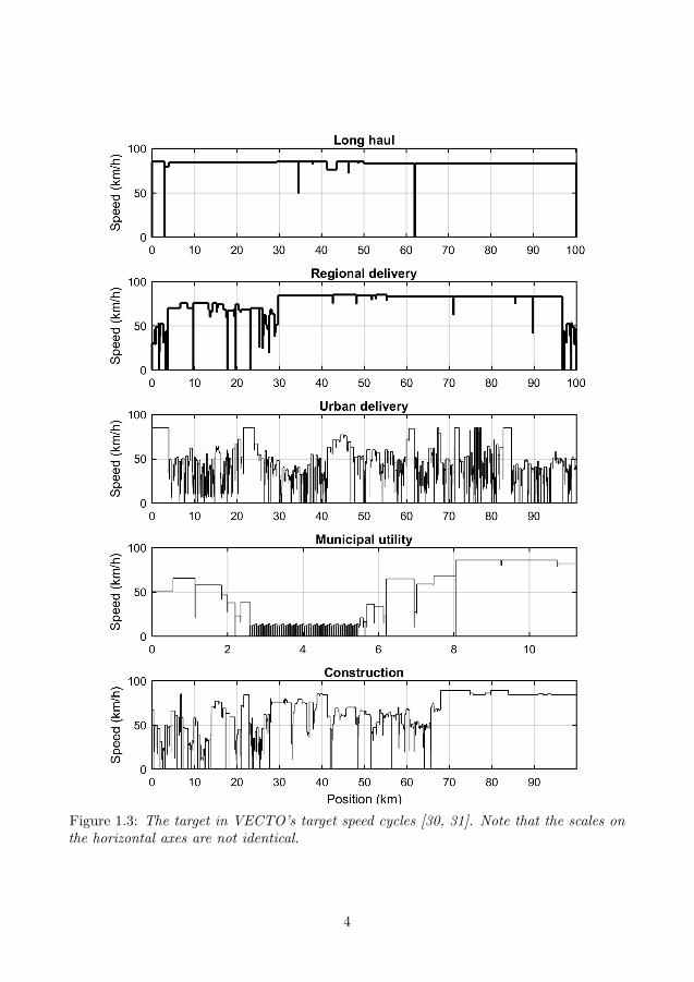
Figure 1.3: The target in VECTO’s target speed cycles [30, 31]. Note that the scales onthe horizontal axes are not identical.

4

entire journals dedicated to the subject.By realistic results, we mean that the virtual model yields the same behaviour when

used in the virtual setting as a physical vehicle does when used in the real world. Thisis a very strict requirement and challenging to achieve. It could be relaxed to insteadstate that the influence from the studied design parameters on the studied vehicle shouldbe similar between the virtual setting and the real world. Unlike the requirement onaccuracy, the requirement on realism includes not only the vehicle but also the thingsthat stimulate it, such as: the driver, the road and the surroundings. Therefore, thesemust be described in the virtual setting, for it to be capable of predicting realistic results.

Comparing this need to the two examples of virtual descriptions encountered so far,there are three problems:

1. Real driving is complex. In some cases, describing it as just a target speed is anoversimplification [42–55]. What would be a more comprehensive description?

2. All vehicles are not operated in the same way. Different applications mean differentdriving conditions [5, 25, 27, 56–59]; a garbage truck typically drives short distances,stop frequently and carries a light payload, while a timber truck may drive longdistances, sometimes in poor road conditions, and often carries a heavy payload.How can such differences be measured and how can applications be compared toassess the similarity?

3. Road and driving conditions change from day to day and induce variation in thevehicle operation [60–70]. Such daily differences disappear when using singularrealisations, no matter what the virtual description looks like. How can this variationbe addressed?

These three problems are necessary to treat to ensure fair comparisons between differentvehicle concepts in a virtual environment. Then the most effective solutions for loweringthe CO2 emissions could be found. That is an excellent setting for product development.On the other hand, if the problems are not considered, technical solutions become moredifficult to develop as the predicted effect may not match the actual one.

This is the background and motivation to the problems that the thesis concerns. Eachproblem deserves a more thorough and scientific inspection than the vague, hand wavingdescription above. Therefore, a short literature survey is presented in Section 1.1.1, thatrelates to the first point, and in Section 1.1.2, that relates to the second and third points.

1.1.1 The inadequacy of driving cycles

What are the concrete problems with using a driving cycle as a mathematical description?An obvious shortcoming is that several physical properties that have a direct effect on thevehicle are missing. The topography (road gradient) is one example, often treated in theliterature [42–49], which has a major impact on energy usage. There are also effects fromthe horizontal geometry (road curvature) [50], the road roughness [51], and the groundconditions: the texture and load bearing capacity [35] (meaning whether it is soft orhard). Apart from the road itself, the surroundings and the mission also affect the energyusage. The weather impacts through wind and temperature [52–54], for example. For

5

VehicleDriver

steering wheel,

pedals

road

properties

road

properties

Operating cycle

sensor gauges,

vehicle position

vehicle

position

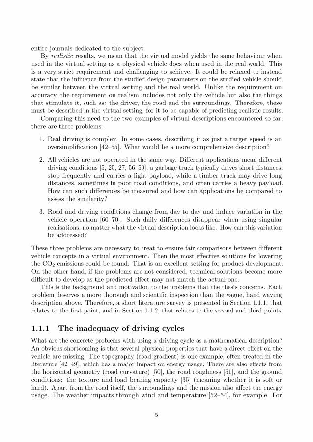
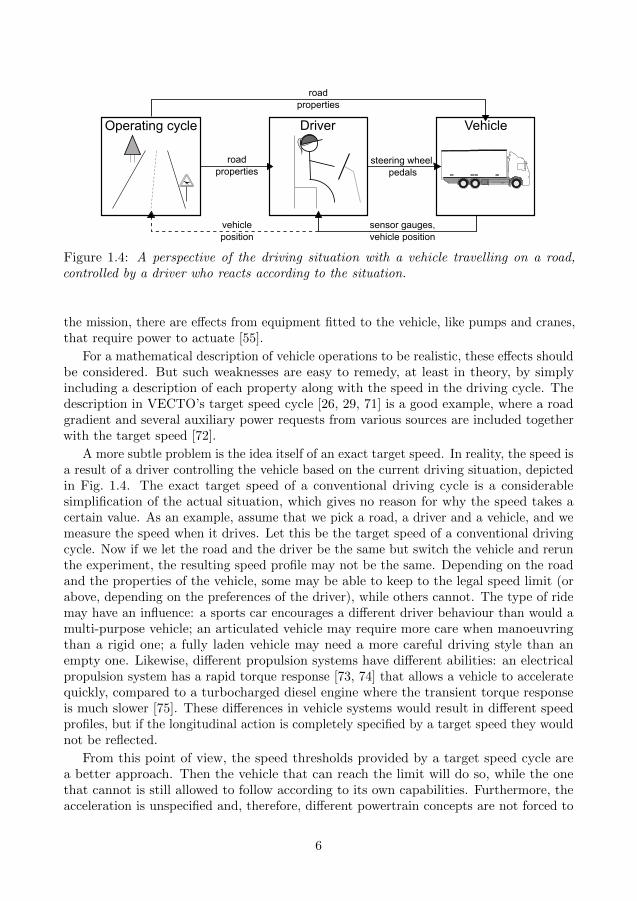
Figure 1.4: A perspective of the driving situation with a vehicle travelling on a road,controlled by a driver who reacts according to the situation.

the mission, there are effects from equipment fitted to the vehicle, like pumps and cranes,that require power to actuate [55].

For a mathematical description of vehicle operations to be realistic, these effects shouldbe considered. But such weaknesses are easy to remedy, at least in theory, by simplyincluding a description of each property along with the speed in the driving cycle. Thedescription in VECTO’s target speed cycle [26, 29, 71] is a good example, where a roadgradient and several auxiliary power requests from various sources are included togetherwith the target speed [72].

A more subtle problem is the idea itself of an exact target speed. In reality, the speed isa result of a driver controlling the vehicle based on the current driving situation, depictedin Fig. 1.4. The exact target speed of a conventional driving cycle is a considerablesimplification of the actual situation, which gives no reason for why the speed takes acertain value. As an example, assume that we pick a road, a driver and a vehicle, and wemeasure the speed when it drives. Let this be the target speed of a conventional drivingcycle. Now if we let the road and the driver be the same but switch the vehicle and rerunthe experiment, the resulting speed profile may not be the same. Depending on the roadand the properties of the vehicle, some may be able to keep to the legal speed limit (orabove, depending on the preferences of the driver), while others cannot. The type of ridemay have an influence: a sports car encourages a different driver behaviour than would amulti-purpose vehicle; an articulated vehicle may require more care when manoeuvringthan a rigid one; a fully laden vehicle may need a more careful driving style than anempty one. Likewise, different propulsion systems have different abilities: an electricalpropulsion system has a rapid torque response [73, 74] that allows a vehicle to acceleratequickly, compared to a turbocharged diesel engine where the transient torque responseis much slower [75]. These differences in vehicle systems would result in different speedprofiles, but if the longitudinal action is completely specified by a target speed they wouldnot be reflected.

From this point of view, the speed thresholds provided by a target speed cycle area better approach. Then the vehicle that can reach the limit will do so, while the onethat cannot is still allowed to follow according to its own capabilities. Furthermore, theacceleration is unspecified and, therefore, different powertrain concepts are not forced to

6

work in the same way.

To point out a second problem with a target speed, independently of whether it comesfrom a conventional driving cycle or a target speed cycle, we come back to the roadproperties that were mentioned before. Take the road curvature as an example: it wasmentioned that the curvature has an effect on the energy usage, but the contribution istwofold. There is a direct effect from energy dissipation due to tyre side slip, but this isgenerally negligible [76]. The greater contribution comes from the indirect effect that thedriver reduces the speed when negotiating a curve [50]. When a target speed is defined bya driving cycle, the indirect (but greater) effect disappears. The road roughness, speedbumps and potholes have similar twofold effects [77].

A third problem appears when considering predictive control systems. There arefunctions that use the vehicle itself as an energy buffer by controlling the speed in a cleverway. For example, systems that can lower the CO2 emissions quite dramatically whennegotiating hills [78–81]. A conventional driving cycle has no freedom in its target speedand therefore no speed variation is possible, rendering any predictive system ineffectual.Clearly this does not allow for a fair comparison between vehicle concepts. In the worstcase it could even be detrimental for product development, as there is little point inspending resources on developing solutions that go uncredited, even though they have areal effect.

A final point to make, is that there is no driver in a driving cycle. The road, theweather and the traffic influence people differently [82] and the person who controls thevehicle has a major impact on its energy usage [83–86].

Most of the cited studies are aware of the weaknesses in using driving cycles to representvehicle operations. Indeed, many suggest techniques to remedy the problems. But theidea of a target speed is still used, though it is patched, changed and extended in differentways. What this thesis tries to do differently, is to step away from the entire concept.Instead we go in another direction and make a new description; one that is firmly basedon the idea that, if we want realistic vehicle behaviour, we need a realistic mathematicaldescription of what affects it.

1.1.2 The differences in application and the variation therein

These issues are quite separate from the driving cycle problem, as they do not concern thedetails of the mathematical transport description but rather the data that it contains. Wewill start by discussing the difficulty with differences in application, and then transitioninto the problem with variation.

The core of the application issue is that a vehicle is not operated in the same way forall missions and geographies [25, 56, 57]. One example of such differences has alreadybeen given: a low speed, frequently stopping garbage truck compared to a heavily ladentimber truck travelling long distances. As an example of the influence from a geographicfeature, consider the topography. It has already been commented that the road gradientimpacts the energy usage [42, 43], so a vehicle mostly operating on flat roads is stimulateddifferently than one that operates mostly in hilly regions [5, 46].

Developing an individual product for every single road and application is not possiblein practice [27]. Instead, a statistical viewpoint is often used. Products and technology

7

65

60

55

50

45

40

fuel consum

ption (

l/10

0 k

m)

Total mass (tonne)

7540 45 50 55 60 65 70

Feb-Mar2012

Apr-Oct

2012

Feb2013

Nov-Jan2012-2013

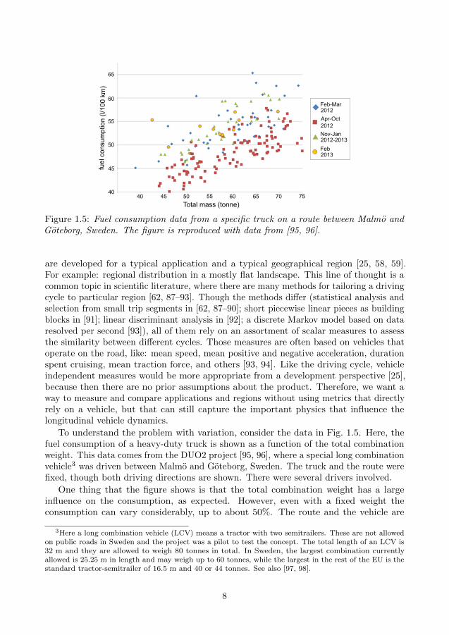
Figure 1.5: Fuel consumption data from a specific truck on a route between Malmo andGoteborg, Sweden. The figure is reproduced with data from [95, 96].

are developed for a typical application and a typical geographical region [25, 58, 59].For example: regional distribution in a mostly flat landscape. This line of thought is acommon topic in scientific literature, where there are many methods for tailoring a drivingcycle to particular region [62, 87–93]. Though the methods differ (statistical analysis andselection from small trip segments in [62, 87–90]; short piecewise linear pieces as buildingblocks in [91]; linear discriminant analysis in [92]; a discrete Markov model based on dataresolved per second [93]), all of them rely on an assortment of scalar measures to assessthe similarity between different cycles. Those measures are often based on vehicles thatoperate on the road, like: mean speed, mean positive and negative acceleration, durationspent cruising, mean traction force, and others [93, 94]. Like the driving cycle, vehicleindependent measures would be more appropriate from a development perspective [25],because then there are no prior assumptions about the product. Therefore, we want away to measure and compare applications and regions without using metrics that directlyrely on a vehicle, but that can still capture the important physics that influence thelongitudinal vehicle dynamics.

To understand the problem with variation, consider the data in Fig. 1.5. Here, thefuel consumption of a heavy-duty truck is shown as a function of the total combinationweight. This data comes from the DUO2 project [95, 96], where a special long combinationvehicle3 was driven between Malmo and Goteborg, Sweden. The truck and the route werefixed, though both driving directions are shown. There were several drivers involved.

One thing that the figure shows is that the total combination weight has a largeinfluence on the consumption, as expected. However, even with a fixed weight theconsumption can vary considerably, up to about 50%. The route and the vehicle are

3Here a long combination vehicle (LCV) means a tractor with two semitrailers. These are not allowedon public roads in Sweden and the project was a pilot to test the concept. The total length of an LCV is32 m and they are allowed to weigh 80 tonnes in total. In Sweden, the largest combination currentlyallowed is 25.25 m in length and may weigh up to 60 tonnes, while the largest in the rest of the EU is thestandard tractor-semitrailer of 16.5 m and 40 or 44 tonnes. See also [97, 98].

8

fixed so this variation appears due to differences in road conditions, traffic, weather anddriving style. To have realistic use cases when developing vehicles, that variation shouldbe considered [60, 61]. The scientific literature offers many ways to introduce variationin vehicle operations using statistical methods [59, 62–70], but these target conventionaldriving cycles.

Both the problems with application and variation need to be approached from astatistical perspective. Whatever solution that is suggested must allow for differenttechnical concepts to reflect their own advantages and disadvantages. Therefore, drivingcycles cannot be a large part of the process. Certainly, they cannot be what the statisticalmeasures are based on, nor the centrepiece of whatever method that is used to introducevariation. Something else is needed.

1.2 Research questions

The three problems can be formally stated as research questions. A fourth question willalso be formulated, to make certain that the solutions to the other three are useful inpractice.

I. How should a transport operation be described mathematically to enable a realisticvehicle usage?

This question refers to the problem of how to make a detailed and comprehensivemathematical description of the driving conditions; one that does not suffer from theproblems that a conventional driving cycle does. The main question can be broken downinto several smaller ones, such as: what physical features should be included? Are thereany important nonphysical features that should be considered? What do the mathematicaldetails look like? How can changes in speed be included without using an explicit targetfunction? Are there any specific principles that the description should follow?

The question intends to deal with transport applications on a basic level but in greatdetail: useful to describe individual roads and missions. We call this ‘the representationproblem’, and it is the first research question.

II. How can transport applications be compared, with respect to geographical andoperational features, in a way that is both vehicle and driver independent?

This question refers to the problem of differences in application, and how to find typicalsimilarities. It requires comparing operations with each other, which implies that scalarmetrics are needed to measure aspects such as: the terrain, the climate, and the mission.Again, the problem can be broken down to smaller questions: what mission features needto be considered? Which ones are the most important for energy usage? How can suitablemetrics be found? Can these be connected to more detailed operation descriptions? Howcan suitable groupings be found?

This question intends to describe transport missions on a high level with few details.We call this ‘the classification problem’, and it is the second research question.

III. How can variation in operation be measured for transport operations, and how canit be reproduced mathematically?

9

This question refers to the problem with variation in everyday usage, and it has two parts.The measurement part has some connection to the second research question: if there aremetrics that can describe transport operations, then a variation could be computed usingelementary mathematical statistics. At least between operations, but not within. Thesecond half of the question, the reproduction part, is very different. Assuming that avariation is known, the question implies that there would need to be a connection from theabstract, high-level description that the classification problem concerns, to the concrete,low-level description that the representation problem addresses. How can this be done?We call this ‘the variation problem’, and it is the third research question.

IV. How should a complete model for dynamic simulations be built to use the detailedmathematical representation of a transport operation, and are there any basicprinciples it should follow?

Simulation has not been discussed in detail so far, but the question is included as a wayto make certain that the solutions to the other problems are useful and robust in practice.Especially the detailed mathematical description in the first research question: this mustbe runnable in a virtual simulation environment so that the energy usage of a vehicledesign can be evaluated. The question concerns technical details surrounding how toimplement the mathematical representation. Whether the problem should be called aresearch question when it really is about technical implementation is a matter of opinion.Nevertheless, we call this ‘the simulation problem’, and it is the fourth and final question.

1.3 Limitations

The thesis concerns problems that are a part of the product development process, thattypically deal with tailoring vehicle components and software functions. Therefore,optimisation is a part of the process too, although located further down the work chain. Infact, the solutions to the research questions are pieces that would go into an optimisationproblem. To really show that the ideas presented here work in practice for the entiredevelopment process, the optimisation part would be needed too. This is a very challengingproblem because the domain is immense, and it has not been attempted in this work. Forideas on how to approach such problems in a vast domain, see [98–100], for example.

The methods that the thesis presents are constructed mostly with heavy-duty trucksin mind. This may not be a severe limitation, since the road is independent of the user.However, some features, like lane width, could be of different relevance depending onwhether the description is used for heavy-duty trucks, passenger cars or motorcycles.Therefore, there may be features of some importance that were overlooked because theywere deemed as less influential for heavy-duty vehicles.

The driver is something else that must be mentioned. It has been explained that for arealistic vehicle behaviour in a virtual model, there needs to be some kind of descriptionof the driver. Modelling this is not trivial. To solve the simulation problem, we will haveto construct a driver model, but it needs to be emphasised that this is not the main pointof the exercise.

10

1.4 Scientific contribution

The main scientific contributions of this work are as follows (listed in order of the papers):

• A case study of the effects of a dual clutch transmission as opposed to a singleclutch transmission on heavy-duty trucks in long haul applications.

• A proposal for a deterministic operating cycle description, independent of the vehicleand the driver, that can include the road, the weather, the traffic and the mission.

• A proposal for a statistical road description, using a framework easily extended toinclude other properties that influence the vehicle operations.

• Insights concerning differences and similarities between the backward method andthe forward method in vehicle simulation models of energy usage.

• Executable models and scripts, written in MATLAB/Simulink, that are public andfree4.

1.5 Thesis outline

The thesis is structured as follows: Chapter 2 outlines what features that need to beincluded in a transport operation description. Three such representations are discussed.It is also shown how these can be connected to each other. The suggested solutionsto the first, second and third research questions are all found here. In Chapter 3, thesimulation model approach is discussed. The suggested solution to the fourth researchquestion is found here. An example with a goods distribution mission and a heavy-dutytruck is also made to showcase how the complete simulation model works in practice.The extended summary finishes with a discussion, some conclusions and possible ideasfor future extensions. The scientific papers on which the thesis is based are appendedafterwards. Figure 1.6 shows how they are related to each other.

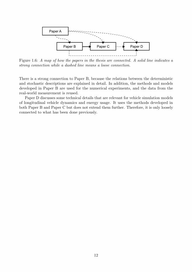
Paper A discusses two transmission technologies, a single clutch gearbox and a dualclutch gearbox, and what effects these have on heavy-duty trucks. Some basic principlesare laid down for how to build a complete simulation model in a forward scheme. Thesereturn throughout all other papers, and that is why the paper has a loose connection(dashed line in Fig. 1.6) to all. Moreover, Volvo trucks’ classification system, the globaltransport application, is discussed. This is an example of a bird’s eye view representation(see Section 2.2).

Paper B introduces the deterministic operating cycle format: the suggested solutionto the first research question. It is also described how to implement the road, missionand driver models, so it treats a part of the solution to the fourth research question too.

Paper C introduces the stochastic operating cycle format, which is a possible solutionto the second research question. It is also explicitly shown how variation can be introducedthrough simulation, and so it contains the suggested solution to the third research question.

4Available through www.chalmers.se/vehprop or directly from https://chalmersuniversity.app.

box.com/s/f5ejzj18bh3c6z057ri71nf04er8g469.

11

www.chalmers.se/vehprop

https://chalmersuniversity.app.box.com/s/f5ejzj18bh3c6z057ri71nf04er8g469

https://chalmersuniversity.app.box.com/s/f5ejzj18bh3c6z057ri71nf04er8g469

Paper A

Paper B Paper C Paper D

Figure 1.6: A map of how the papers in the thesis are connected. A solid line indicates astrong connection while a dashed line means a loose connection.

There is a strong connection to Paper B, because the relations between the deterministicand stochastic descriptions are explained in detail. In addition, the methods and modelsdeveloped in Paper B are used for the numerical experiments, and the data from thereal-world measurement is reused.

Paper D discusses some technical details that are relevant for vehicle simulation modelsof longitudinal vehicle dynamics and energy usage. It uses the methods developed inboth Paper B and Paper C but does not extend them further. Therefore, it is only looselyconnected to what has been done previously.

12

2 Representing transport operations

The main focal point in this chapter is how to describe transport operations. It will bedone in three ways: a high-level view with a modest amount of detail, a low-level viewwith a great amount of detail, and something in between, an intermediate view with amoderate amount of detail. All three serve as representations of transport operations,but they are used in different ways. Before getting into the representations though, thereare a couple of expressions that need to be defined.

We define the transport application as the overall purpose of a vehicle during itslifetime. This refers to a very broad, rough way of talking about everything a certainvehicle does. Examples of transport applications would be: long distance cargo transport,recycling and garbage transport, regional distribution, city bus, intra city bus, and manyothers. Unfortunately, the definition cannot be made much more rigorous than that,because the concept itself is vague, as the examples above show.

We define the transport operation as an enumerable number of tasks along a specificroute. Typically, the concept refers to the driving that a vehicle does during singularinstances, like a day. It could be interpreted as shorter parts too, like the driving between apick up and drop off location. If all transport operations that a vehicle executes during itslifetime are collected, then this would correspond to the transport application. Moreover,a transport operation can be broken down into the road, the surroundings, the weather,other vehicles and the tasks themselves, which we come to next.

We define the transport mission as the details surrounding the tasks of a transportoperation. This include their position, the payload, the flow of power, the direction ofdriving, and similar features that relate to the purpose of the transport. Thus, eachtransport operation comes with a mission. Of course, it could be very simple and onlyconsist of the starting and ending positions.

The material in this chapter is, for the most part, already explained in the papers.Paper A mentions a particular example of the bird’s eye view, the main topic in Paper Bis the deterministic view and the main topic in Paper C is the statistical view. Allperspectives are also mentioned in [101] to some extent.

2.1 What features need to be included?

Independently of which level of detail that is considered, we first need to figure outwhat features, meaning either physical phenomena or assumptions, and actions of thetransport environment that need to be included. Plenty of examples are mentioned bythe scientific works referenced in Chapter 1, although it is not too difficult to motivatethem mathematically, by applying the laws of classical mechanics to a vehicle moving ona road.

Consider the free body diagram (FBD) of a two-axle truck in Fig. 2.1 (left) and ageneric axle (right). For the vehicle, the aerodynamic resistance, gravitational force, frontand rear traction forces, and front and rear normal forces are shown. For the genericaxle, a total external torque (combined propulsion and brake torque) is drawn and thenormal force is offset by small distance frR. The suspension has been approximated as

13

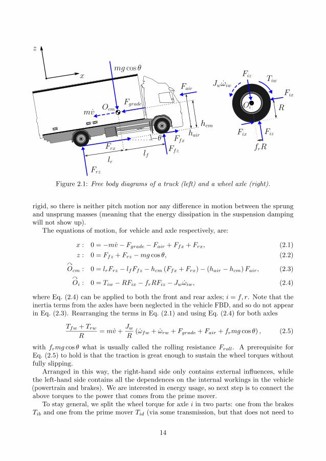
Figure 2.1: Free body diagrams of a truck (left) and a wheel axle (right).

rigid, so there is neither pitch motion nor any difference in motion between the sprungand unsprung masses (meaning that the energy dissipation in the suspension dampingwill not show up).

The equations of motion, for vehicle and axle respectively, are:

x : 0 = −mv − Fgrade − Fair + Ffx + Frx, (2.1)

z : 0 = Ffz + Frz −mg cos θ, (2.2)yOcm : 0 = lrFrz − lfFfz − hcm (Ffx + Frx)− (hair − hcm)Fair, (2.3)

yOi : 0 = Tiw −RFix − frRFiz − Jwωiw, (2.4)

where Eq. (2.4) can be applied to both the front and rear axles; i = f, r. Note that theinertia terms from the axles have been neglected in the vehicle FBD, and so do not appearin Eq. (2.3). Rearranging the terms in Eq. (2.1) and using Eq. (2.4) for both axles

Tfw + TrwR

= mv +JwR

(ωfw + ωrw + Fgrade + Fair + frmg cos θ) , (2.5)

with frmg cos θ what is usually called the rolling resistance Froll. A prerequisite forEq. (2.5) to hold is that the traction is great enough to sustain the wheel torques withoutfully slipping.

Arranged in this way, the right-hand side only contains external influences, whilethe left-hand side contains all the dependences on the internal workings in the vehicle(powertrain and brakes). We are interested in energy usage, so next step is to connect theabove torques to the power that comes from the prime mover.

To stay general, we split the wheel torque for axle i in two parts: one from the brakesTib and one from the prime mover Tid (via some transmission, but that does not need to

14

be resolved at the moment)Tiw = Tid − Tib. (2.6)

In which case we can write the power needed to move the vehicle Pd as

Pd = ωfwTfd + ωrwTrd. (2.7)

The prime mover may also need to supply a power Paux to the auxiliary equipment,meaning things that are intrinsic to the vehicle, such as air condition, and a power PPTO

to any mission specific equipment, like a crane or a refrigerator. The total power thatneeds to be supplied is

Ptot = Pd + Paux + PPTO. (2.8)

Note that we have tried to stay fairly general here, so the expressions in Eqs. (2.5) to (2.7)are slightly messy. They could be made clearer (and probably more familiar) by makingsome approximations. If it is assumed that there is a propulsion torque Td on one axleonly (which one does not matter, for this argument), that the brake torques are zero,and neglect any longitudinal tyre slip so that ωfw = ωrw = v/R, then Eqs. (2.5) to (2.7)reduce to

Ptot = v (Finertia + Fgrade + Fair + Froll) + Paux + PPTO. (2.9)

Where term Finertia contains the mass as well as the inertia of the axles (the effectivemass m∗).

For a description of the surroundings to be realistic, a fundamental requirement is thatit must excite the vehicle with the right things. We can understand that quantitatively bylooking at the right-hand side of Eq. (2.9). Let’s interpret these in terms of the physicalproperties of the road, the surroundings and mission actions.

• The inertia term: Finertia = m∗v.This term depends on mass and the change in speed. The mass is straightforward todeal with: apart from the vehicle itself, it includes the payload which is a part of themission. We will need to know what the payload is and how it changes. The speedchanges are a much more complicated subject, because they arise from a multitudeof sources. On the road, the speed signs, stop signs, give way signs, traffic lights,speed bumps, potholes, curves and road surface all require the driver to adapt thespeed. Likewise, other vehicles can cause rapid changes in the speed.

• The road gradient: Fgrade = mg sin (−θ).Another mass dependent term, this time coupled with road gradient angle θ. Sinceboth the mass and the gravitational acceleration are included, the term is large inmagnitude and the road gradient often has a great influence on the energy usage.Thus, the angle needs to be included in some form. The choice of direction is inaccordance with the convention in ISO 8855 [102].

• The rolling resistance: Froll = frmg cos θ.The mass and road gradient angle have been mentioned already, but the rollingresistance coefficient fr depends on the ground properties. These need to be includedin some form. Additionally, the weather can have an impact, by changing the surfacelayer: making it wet, or covering it with ice or snow.

15

• The aerodynamic resistance: Fair = ρCdA|vr|vr/2.The new parts here that depend on the external influences are the density of air ρand the relative speed vr between the vehicle and the air. The air density depends onthe weather through the atmospheric pressure, ambient temperature and humidity.The wind is a weather effect, while the road properties that are the greatest influenceon the vehicle speed were already mentioned under the inertia term.

• The power terms: Paux and PPTO.The power terms are direct parasites on the vehicle energy source. The powertake-off is mission dependent, so any external equipment needs to be considered.The auxiliary power term is more questionable, it is rather a property of the vehicleitself than a result of external influences. We therefore refrain from including anauxiliary power in the description of the mission. Note though that there couldbe indirect dependences, for example the ambient temperature could affect thepower by changing the need for cooling or heating. Such influences should still beaccounted for.

The above list of features is not exhaustive by any means and there are more influences thanthose described by Eq. (2.9). For example, there are direct effects from the curvature dueto side slipping and from the road roughness due to energy dissipation in the suspensiondamping. These appear when the vehicle motion is treated more comprehensively thanwith the planar, two-dimensional model in Eqs. (2.1) to (2.4).

The travel distance did not show up under any of the terms in the above list, thoughit influences the total work W

W =

L∫

0

Fdx ds, (2.10)

with Fdx the propulsion force on whichever axle (or the sum, if both) that is propelledand L the mission distance.

Now we know of a number of properties that should be taken into consideration whenconstructing a road description, independently of its level of detail. It is also importantthat there is no dependence on the vehicle itself, and preferably not the driver either.Vehicle independence is central to the idea of making a description of the operation thatallows for realistic behaviour, no matter what vehicle that is used. Driver independenceis also desirable, because then the impact from the environment and that from the drivercan be varied independently.

2.2 A high-level description for classification

The first description that we will discuss is a very rough and highly generalising one,almost colloquial in nature. We call this a bird’s eye view, because the purpose is togive an overview of entire transport applications, without going deeply into details. Thematerial connects to the second research question.

One reason for why this kind of description is needed has already been mentioned: it

16

is not feasible to develop products for singular roads or individual users1. Instead, onewould want to develop products for applications that are similar with respect to theirtasks and the landscapes in which they are set. Therefore, there is a need for some wayto compare applications and determine what is similar and what is not. This could bedone with a high-level description than gives a rough overview.

A second reason for why a broad description is needed, is when discussing with auser how to outfit a vehicle. In that case, it is not a question of product developmentbut selection: to choose the best combination of components and functions. To do so,something must be known about what kind of application the user has in mind. Thisis why the tone should be colloquial: all users cannot be expected to have full insightinto complicated models and parameters. Rather, the language should be familiar andintuitive, if possible. Still, clear definitions are vital, and could be supplied by a high-leveldescription.

A broad description is thus a kind of classification system, where a transport applicationis labelled with respect to different categories and grouped with those of a similar nature.Three things are needed for a system like that:

1. A list of categories that make up the classification system.

For a classification connected to the energy usage of a vehicle, the relevant categorieswould be the features mentioned in Section 2.1. However, there are more vehicleproperties than energy usage that are of interest for product development, likefatigue. Therefore, a broad classification system would rather target the completelongitudinal vehicle behaviour. It can later be clarified which categories that impactwhich vehicle property the most.

2. A number of labels (i.e. values, classes or groups) for every category.

How many labels and what they should be would have to depend on the categoryin question. If a low resolution is enough, then two groups would be sufficient:separating between high and low values. If a higher resolution is needed, then moregroups are simply added.

3. A method to measure a transport application with respect to the categories.

This implies that each category must be associated with some kind of distancefunction: a metric. What this should be would again have to depend on the categoryin question. Moreover, once a metric has been found, it must be used to find suitablecriteria for the labels.

Constructing such a system is quite an undertaking. Furthermore, it is far fromobvious how to satisfy points 2 and 3 above for every category listed in Section 2.1. Toshow one possible approach, we can make an example with a single feature. This ad hocapproach will have many weaknesses, which will be commented on afterwards.

Let’s say that we want to construct a classification parameter for the mission distance.First of all, we should think about what impact the feature has and what the classificationparameter actually says about the transport application. The mission distance affects

1Although there are exceptions, like the research project in [103].

17

the total energy through Eq. (2.10), but energy usage is usually considered per distanceunit, just like fuel consumption and CO2 emissions, in which case the total distance isunimportant. There are some cases where it has a secondary effect, for instance: if avehicle has an energy buffer that is relatively limited in size (like a battery), but overallthe distance is not of primary importance for energy consumption. However, when itcomes to longitudinal vehicle behaviour in general, it can be expected that the missiondistance is characteristic for certain groups of applications. For example, it could be usedto separate between applications resembling long-haul and applications resembling urbandistribution. Therefore, a mission distance parameter could have some usefulness.

Next, the labels need to be invented. The terminology should be familiar, therefore saythat we decide on using three distance classes and call them: ‘short’, ‘medium’ and ‘long’.The third step is to find the metric, preferably one that is easy to work with. One optionis to use the mean travel distance per operation: it is a simple concept to understand anda user should have some idea of how long a distance they usually go. Furthermore, if it isa matter of replacing a truck, there could be data available. It seems likely that the traveldistance would be available as a signal and the average distance could then be estimated.

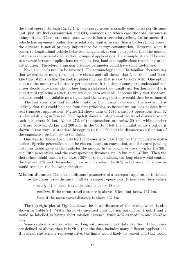
The last step is to find suitable limits for the classes in terms of the metric. It isunlikely that this could be done from first principles, so instead we can look at data fromreal transport applications. Figure 2.2 shows data of 1684 transport operations from 32trucks, all driving in Europe. The top left shows a histogram of the travel distance, whereeach bar covers 20 km. About 27% of the operations are below 20 km, while another65% are between 20 km and 200 km. In the bottom left the cumulative distribution isshown in two ways: a standard histogram to the left, and the distance as a function ofthe cumulative probability to the right.

One way to choose the limits for the classes is to base them on the cumulative distri-bution. Specific percentiles could be chosen, based on convention, and the correspondingdistances would serve as the limits for the groups. In the plot, lines are shown for the 30thand 70th percentiles, and the corresponding distances are 18 km and 137 km. Then theshort class would contain the lowest 30% of the operations, the long class would containthe highest 30% and the medium class would contain the 40% in between. This processwould result in the following definition:

Mission distance The mission distance parameter of a transport application is definedas the mean travel distance of all its transport operations. It may take three values:

– short, if the mean travel distance is below 18 km.

– medium, if the mean travel distance is above 18 km, but below 137 km.

– long, if the mean travel distance is above 137 km.

The top right plot of Fig. 2.2 shows the mean distance of the trucks, which is alsoshown in Table 2.1. With the newly invented classification parameter, truck 1 and 2would be labelled as having short mission distance, truck 3-25 as medium and 26-32 aslong.

Some caution is advised when working with measurement data like this. If the classesare defined as above, then it is vital that the data includes many different applications.If it is not statistically representative, the limits would likely be biased and that would

18

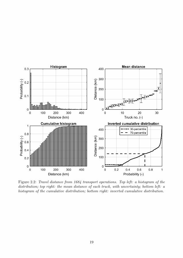
Figure 2.2: Travel distance from 1684 transport operations. Top left: a histogram of thedistribution; top right: the mean distance of each truck, with uncertainty; bottom left: ahistogram of the cumulative distribution; bottom right: inverted cumulative distribution.

19

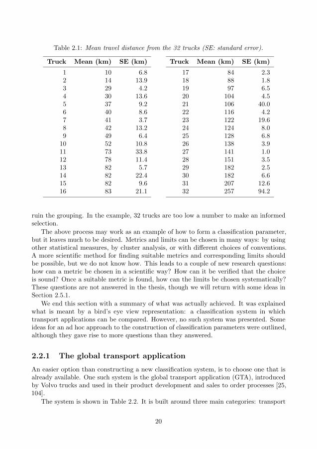
Table 2.1: Mean travel distance from the 32 trucks (SE: standard error).

Truck Mean (km) SE (km) Truck Mean (km) SE (km)

1 10 6.8 17 84 2.32 14 13.9 18 88 1.83 29 4.2 19 97 6.54 30 13.6 20 104 4.55 37 9.2 21 106 40.06 40 8.6 22 116 4.27 41 3.7 23 122 19.68 42 13.2 24 124 8.09 49 6.4 25 128 6.8

10 52 10.8 26 138 3.911 73 33.8 27 141 1.012 78 11.4 28 151 3.513 82 5.7 29 182 2.514 82 22.4 30 182 6.615 82 9.6 31 207 12.616 83 21.1 32 257 94.2

ruin the grouping. In the example, 32 trucks are too low a number to make an informedselection.

The above process may work as an example of how to form a classification parameter,but it leaves much to be desired. Metrics and limits can be chosen in many ways: by usingother statistical measures, by cluster analysis, or with different choices of conventions.A more scientific method for finding suitable metrics and corresponding limits shouldbe possible, but we do not know how. This leads to a couple of new research questions:how can a metric be chosen in a scientific way? How can it be verified that the choiceis sound? Once a suitable metric is found, how can the limits be chosen systematically?These questions are not answered in the thesis, though we will return with some ideas inSection 2.5.1.

We end this section with a summary of what was actually achieved. It was explainedwhat is meant by a bird’s eye view representation: a classification system in whichtransport applications can be compared. However, no such system was presented. Someideas for an ad hoc approach to the construction of classification parameters were outlined,although they gave rise to more questions than they answered.

2.2.1 The global transport application

An easier option than constructing a new classification system, is to choose one that isalready available. One such system is the global transport application (GTA), introducedby Volvo trucks and used in their product development and sales to order processes [25,104].

The system is shown in Table 2.2. It is built around three main categories: transport

20

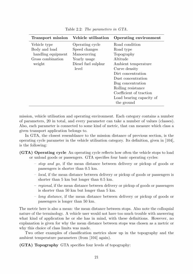
Table 2.2: The parameters in GTA.

Transport mission Vehicle utilisation Operating environment

Vehicle type Operating cycle Road conditionBody and loadhandling equipment

Speed changes Road typeManoeuvring Topography

Gross combinationweight

Yearly usage AltitudeDiesel fuel sulphurlevel

Ambient temperatureCurve densityDirt concentrationDust concentrationBug concentrationRolling resistanceCoefficient of tractionLoad bearing capacity ofthe ground

mission, vehicle utilisation and operating environment. Each category contains a numberof parameters, 20 in total, and every parameter can take a number of values (classes).Also, each parameter is connected to some kind of metric, that can measure which class agiven transport application belongs to.

In GTA, the closest resemblance to the mission distance of previous section, is theoperating cycle parameter in the vehicle utilisation category. Its definition, given in [104],is the following:

(GTA) Operating cycle An operating cycle reflects how often the vehicle stops to loador unload goods or passengers. GTA specifies four basic operating cycles:

– stop and go, if the mean distance between delivery or pickup of goods orpassengers is shorter than 0.5 km.

– local, if the mean distance between delivery or pickup of goods or passengers isshorter than 5 km but longer than 0.5 km.

– regional, if the mean distance between delivery or pickup of goods or passengersis shorter than 50 km but longer than 5 km.

– long distance, if the mean distance between delivery or pickup of goods orpassengers is longer than 50 km.

The metric here is also a mean: the mean distance between stops. Also note the colloquialnature of the terminology. A vehicle user would not have too much trouble with answeringwhat kind of application he or she has in mind, with these definitions. However, noexplanation is given for why the mean distance between stops was chosen as a metric orwhy this choice of class limits was made.

Two other examples of classification metrics show up in the topography and theambient temperature parameters (from [104] again).

(GTA) Topography GTA specifies four levels of topography:

21

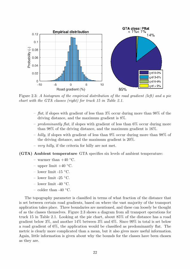
Figure 2.3: A histogram of the empirical distribution of the road gradient (left) and a piechart with the GTA classes (right) for truck 15 in Table 2.1.

– flat, if slopes with gradient of less than 3% occur during more than 98% of thedriving distance, and the maximum gradient is 8%.

– predominantly flat, if slopes with gradient of less than 6% occur during morethan 98% of the driving distance, and the maximum gradient is 16%.

– hilly, if slopes with gradient of less than 9% occur during more than 98% ofthe driving distance, and the maximum gradient is 20%.

– very hilly, if the criteria for hilly are not met.

(GTA) Ambient temperature GTA specifies six levels of ambient temperature:

– warmer than +40 ◦C.

– upper limit +40 ◦C.

– lower limit -15 ◦C.



– colder than -40 ◦C.

The topography parameter is classified in terms of what fraction of the distance thatis set between certain road gradients, based on where the vast majority of the transportapplication takes place. Three boundaries are mentioned, and these can loosely be thoughtof as the classes themselves. Figure 2.3 shows a diagram from all transport operations fortruck 15 in Table 2.1. Looking at the pie chart, about 85% of the distance has a roadgradient below 3%, and another 14% between 3% and 6%. Since 99% in total is set belowa road gradient of 6%, the application would be classified as predominantly flat. Themetric is clearly more complicated than a mean, but it also gives more useful information.Again, little information is given about why the bounds for the classes have been chosenas they are.

22

The classification method in the ambient temperature parameter is of a different kind:it is not statistical in nature but just a fixed limit. A reason why could be that thephysical influence of the parameter (temperature, in this case) is rather weak. A simplechoice of metric could be a good idea just to avoid spending unnecessary time and effort.

GTA is one example of a bird’s eye view classification system, but there are others:topography in [44], curvature in [105], or [106] for a combination. Other vehicle manufac-turers may have their own systems, although they are not public. For instance, Scaniahas a system based on what they call user factors, briefly mentioned in Chapter 4 of [107].

Before leaving GTA, it should be pointed out that many of the parameters in Table 2.2are more or less irrelevant for energy consumption, for example: yearly usage. This isbecause GTA is an overall description of the transport application, that can be usedwhen considering many vehicle properties. This was mentioned before but is worth toemphasise with this functional classification system as an explicit example.

2.3 A mid-level description for variation

Now we turn to a more comprehensive statistical description of either individual transportoperations or several in a collection. The material in this section is a summary of thestudy in Paper C and connects to the third research question.

While the classification system of a bird’s eye view can be based on metrics that arestatistical in nature, like the mean travel distance, these are meant to describe entiretransport applications. Its metrics are supposed to be rough tools only. Furthermore, thevariation problem in the research question cannot be solved with a bird’s eye view systemthat leans on mean values, because those say nothing about variation. Something else isneeded.

Many of the approaches found in scientific literature that deal with uncertainty andvariation of CO2 emissions use stochastic processes [59, 62–70]. These studies havemostly focused on driving cycles, whereas we need to consider the properties mentionedin Section 2.1. The approach with stochastic processes holds merit though. If modellingsomething as a random process, then probability and variation appear naturally. Thattrait would suit our needs perfectly.

2.3.1 Modelling individual road properties

To limit the scope, we will not consider all properties that were mentioned in Section 2.1,but only the ones that are associated with the road itself. These are: stop and give waysigns, traffic lights, speed bumps, speed signs, ground type, topography, curvature androad roughness. For some, suitable stochastic models have already been designed byothers.

The road curvature (horizontal geometry) was modelled by Karlsson [108, 109] as amarked Poisson process and by Maghsood et al [110–112] as a hidden Markov model. Theapplication was not energy usage but fatigue assessment of steering components, but thecharacteristics of the road remain the same. The topography was treated statisticallyby Rouillard and Sek [113] and more recently by Johannesson et al [114, 115], whomodelled it as a first order autoregressive relation with either a Gaussian or Laplacian

23

signature. When the road roughness is treated through the spectral power density of thevertical profiled, as recommended by ISO 8608 [116], stochastic models have been used forquite some time [117]. Bogsjo [118] and Johannesson et al [119] noted that the commonapproach with a Gaussian process could be improved over longer distances and suggesteda model with a Laplacian signature. In summary: the curvature, topography and roadroughness do not need to be modelled from scratch.

To model the others, let’s say that a transport operation of length L is given. Nowconsider only the road itself. Let the road properties be individually described by asequence of variables, discrete or continuous, just like what one would get if measuringat given points. We will see these sequences as containing random variables2 and modelthem by the simplest stochastic process that fits the behaviour. At first, we will assumethat the sequences are mutually independent, so that, for example, the speed signs are notaffected by curvature and vice versa. The assumption will be revised later in Section 2.3.2.

Stop signs, give way signs, traffic lights, and speed bumps

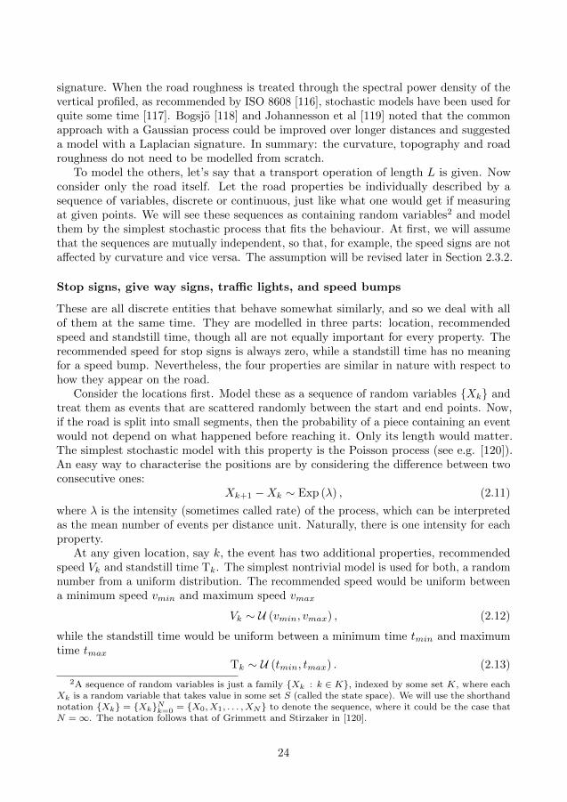
These are all discrete entities that behave somewhat similarly, and so we deal with allof them at the same time. They are modelled in three parts: location, recommendedspeed and standstill time, though all are not equally important for every property. Therecommended speed for stop signs is always zero, while a standstill time has no meaningfor a speed bump. Nevertheless, the four properties are similar in nature with respect tohow they appear on the road.

Consider the locations first. Model these as a sequence of random variables {Xk} andtreat them as events that are scattered randomly between the start and end points. Now,if the road is split into small segments, then the probability of a piece containing an eventwould not depend on what happened before reaching it. Only its length would matter.The simplest stochastic model with this property is the Poisson process (see e.g. [120]).An easy way to characterise the positions are by considering the difference between twoconsecutive ones:

Xk+1 −Xk ∼ Exp (λ) , (2.11)

where λ is the intensity (sometimes called rate) of the process, which can be interpretedas the mean number of events per distance unit. Naturally, there is one intensity for eachproperty.

At any given location, say k, the event has two additional properties, recommendedspeed Vk and standstill time Tk. The simplest nontrivial model is used for both, a randomnumber from a uniform distribution. The recommended speed would be uniform betweena minimum speed vmin and maximum speed vmax

Vk ∼ U (vmin, vmax) , (2.12)

while the standstill time would be uniform between a minimum time tmin and maximumtime tmax

Tk ∼ U (tmin, tmax) . (2.13)

2A sequence of random variables is just a family {Xk : k ∈ K}, indexed by some set K, where eachXk is a random variable that takes value in some set S (called the state space). We will use the shorthandnotation {Xk} = {Xk}Nk=0 = {X0, X1, . . . , XN} to denote the sequence, where it could be the case thatN = ∞. The notation follows that of Grimmett and Stirzaker in [120].

24

The five numbers describing the intensity, recommended speed and standstill time bounds,fully parametrise the model. Again: the stop sign and speed bump models only use three.

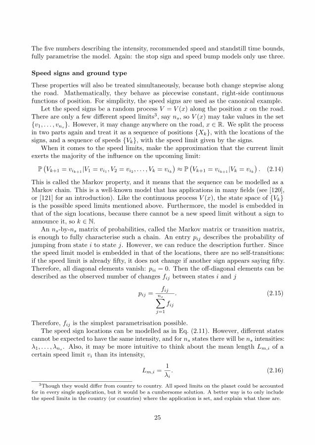
Speed signs and ground type

These properties will also be treated simultaneously, because both change stepwise alongthe road. Mathematically, they behave as piecewise constant, right-side continuousfunctions of position. For simplicity, the speed signs are used as the canonical example.

Let the speed signs be a random process V = V (x) along the position x on the road.There are only a few different speed limits3, say ns, so V (x) may take values in the set{v1, . . . , vns}. However, it may change anywhere on the road, x ∈ R. We split the processin two parts again and treat it as a sequence of positions {Xk}, with the locations of thesigns, and a sequence of speeds {Vk}, with the speed limit given by the signs.

When it comes to the speed limits, make the approximation that the current limitexerts the majority of the influence on the upcoming limit:

P(Vk+1 = vik+1

|V1 = vi1 , V2 = vi2 , . . . , Vk = vik)≈ P

(Vk+1 = vik+1

|Vk = vik). (2.14)

This is called the Markov property, and it means that the sequence can be modelled as aMarkov chain. This is a well-known model that has applications in many fields (see [120],or [121] for an introduction). Like the continuous process V (x), the state space of {Vk}is the possible speed limits mentioned above. Furthermore, the model is embedded inthat of the sign locations, because there cannot be a new speed limit without a sign toannounce it, so k ∈ N.

An ns-by-ns matrix of probabilities, called the Markov matrix or transition matrix,is enough to fully characterise such a chain. An entry pij describes the probability ofjumping from state i to state j. However, we can reduce the description further. Sincethe speed limit model is embedded in that of the locations, there are no self-transitions:if the speed limit is already fifty, it does not change if another sign appears saying fifty.Therefore, all diagonal elements vanish: pii = 0. Then the off-diagonal elements can bedescribed as the observed number of changes fij between states i and j

pij =fij

ns∑

j=1

fij

. (2.15)

Therefore, fij is the simplest parametrisation possible.The speed sign locations can be modelled as in Eq. (2.11). However, different states

cannot be expected to have the same intensity, and for ns states there will be ns intensities:λ1, . . . , λns . Also, it may be more intuitive to think about the mean length Lm,i of acertain speed limit vi than its intensity,

Lm,i =1

λi. (2.16)

3Though they would differ from country to country. All speed limits on the planet could be accountedfor in every single application, but it would be a cumbersome solution. A better way is to only includethe speed limits in the country (or countries) where the application is set, and explain what these are.

25

The complete description thus consists of the matrix fij and the ns mean lengths Lm,i.The ground type works the same as the speed signs, but it has a different number of

states ng, with types {g1, . . . , gng}, where g1 could be tarmac, g2 gravel, and so on. Each

state is also associated with a load bearing capacity, but this can be taken as a propertyof the states themselves and does not need a random process.

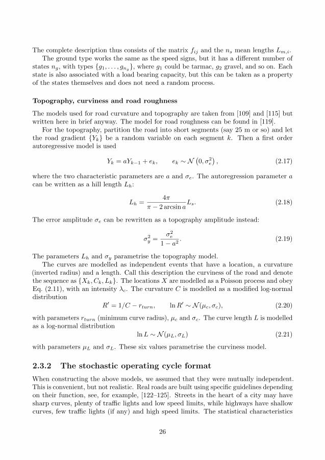
Topography, curviness and road roughness

The models used for road curvature and topography are taken from [109] and [115] butwritten here in brief anyway. The model for road roughness can be found in [119].

For the topography, partition the road into short segments (say 25 m or so) and letthe road gradient {Yk} be a random variable on each segment k. Then a first orderautoregressive model is used

Yk = aYk−1 + ek, ek ∼ N(0, σ2

e

), (2.17)

where the two characteristic parameters are a and σe. The autoregression parameter acan be written as a hill length Lh:

Lh =4π

π − 2 arcsin aLs. (2.18)

The error amplitude σe can be rewritten as a topography amplitude instead:

σ2y =

σ2e

1− a2 . (2.19)

The parameters Lh and σy parametrise the topography model.The curves are modelled as independent events that have a location, a curvature

(inverted radius) and a length. Call this description the curviness of the road and denotethe sequence as {Xk, Ck, Lk}. The locations X are modelled as a Poisson process and obeyEq. (2.11), with an intensity λc. The curvature C is modelled as a modified log-normaldistribution

R′ = 1/C − rturn, lnR′ ∼ N (µc, σc), (2.20)

with parameters rturn (minimum curve radius), µc and σc. The curve length L is modelledas a log-normal distribution

lnL ∼ N (µL, σL) (2.21)

with parameters µL and σL. These six values parametrise the curviness model.

2.3.2 The stochastic operating cycle format

When constructing the above models, we assumed that they were mutually independent.This is convenient, but not realistic. Real roads are built using specific guidelines dependingon their function, see, for example, [122–125]. Streets in the heart of a city may havesharp curves, plenty of traffic lights and low speed limits, while highways have shallowcurves, few traffic lights (if any) and high speed limits. The statistical characteristics

26

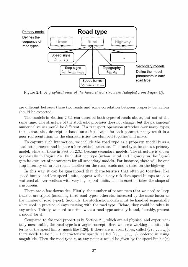
Road type

Speed bumps

Stop signs Topography

Speed signs…

RuralUrban Highway

Secondary models

parameters in each

Define the model

road type

Primary model

sequence of

Defines the

road types

Figure 2.4: A graphical view of the hierarchical structure (adapted from Paper C).

are different between these two roads and some correlation between property behaviourshould be expected.

The models in Section 2.3.1 can describe both types of roads above, but not at thesame time. The structure of the stochastic processes does not change, but the parameters’numerical values would be different. If a transport operation stretches over many types,then a statistical description based on a single value for each parameter may result in apoor representation, as the characteristics are clumped together and mixed.

To capture such interaction, we include the road type as a property, model it as astochastic process, and impose a hierarchical structure. The road type becomes a primarymodel, while all those in Section 2.3.1 become secondary models. The structure is showngraphically in Figure 2.4. Each distinct type (urban, rural and highway, in the figure)gets its own set of parameters for all secondary models. For instance, there will be onestop intensity on urban roads, another on the rural roads and a third on the highway.

In this way, it can be guaranteed that characteristics that often go together, likespeed bumps and low speed limits, appear without any risk that speed bumps are alsoscattered all over sections with very high speed limits. The interaction takes the shape ofa grouping.

There are a few downsides. Firstly, the number of parameters that we need to keeptrack of are tripled (assuming three road types, otherwise increased by the same factor asthe number of road types). Secondly, the stochastic models must be handled sequentiallywhen used in practice, always starting with the road type. Before, they could be taken inany order. Thirdly, we need to define what a road type actually is and, fourthly, presenta model for it.

Compared to the road properties in Section 2.1, which are all physical and experimen-tally measurable, the road type is a vague concept. Here we use a working definition interms of the speed limits, much like [126]. If there are nr road types, called {r1, . . . , rnr},there needs to be nr − 1 characteristic speeds, called {v1, . . . , vnr−1}, ordered in risingmagnitude. Then the road type rt at any point x would be given by the speed limit v(x)

27

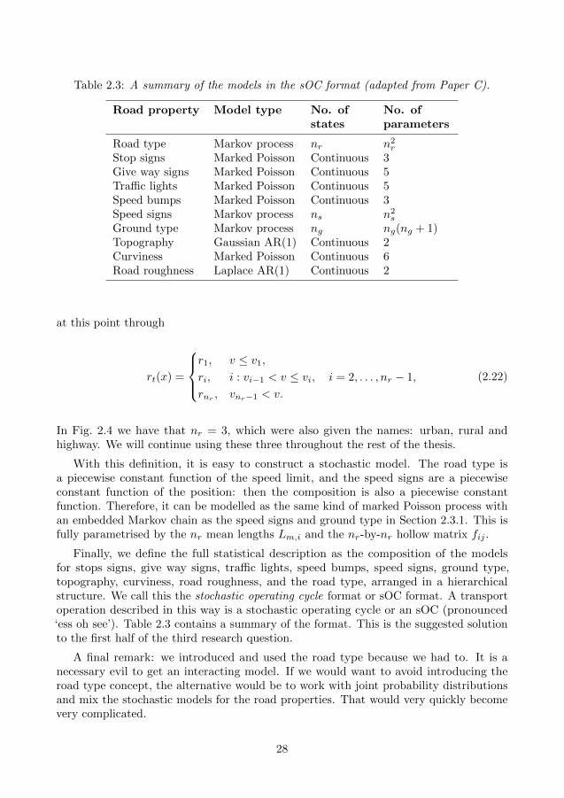
Table 2.3: A summary of the models in the sOC format (adapted from Paper C).

Road property Model type No. ofstates

No. ofparameters

Road type Markov process nr n2rStop signs Marked Poisson Continuous 3Give way signs Marked Poisson Continuous 5Traffic lights Marked Poisson Continuous 5Speed bumps Marked Poisson Continuous 3Speed signs Markov process ns n2sGround type Markov process ng ng(ng + 1)Topography Gaussian AR(1) Continuous 2Curviness Marked Poisson Continuous 6Road roughness Laplace AR(1) Continuous 2

at this point through

rt(x) =

r1, v ≤ v1,ri, i : vi−1 < v ≤ vi, i = 2, . . . , nr − 1,

rnr, vnr−1 < v.

(2.22)

In Fig. 2.4 we have that nr = 3, which were also given the names: urban, rural andhighway. We will continue using these three throughout the rest of the thesis.

With this definition, it is easy to construct a stochastic model. The road type isa piecewise constant function of the speed limit, and the speed signs are a piecewiseconstant function of the position: then the composition is also a piecewise constantfunction. Therefore, it can be modelled as the same kind of marked Poisson process withan embedded Markov chain as the speed signs and ground type in Section 2.3.1. This isfully parametrised by the nr mean lengths Lm,i and the nr-by-nr hollow matrix fij .

Finally, we define the full statistical description as the composition of the modelsfor stops signs, give way signs, traffic lights, speed bumps, speed signs, ground type,topography, curviness, road roughness, and the road type, arranged in a hierarchicalstructure. We call this the stochastic operating cycle format or sOC format. A transportoperation described in this way is a stochastic operating cycle or an sOC (pronounced‘ess oh see’). Table 2.3 contains a summary of the format. This is the suggested solutionto the first half of the third research question.

A final remark: we introduced and used the road type because we had to. It is anecessary evil to get an interacting model. If we would want to avoid introducing theroad type concept, the alternative would be to work with joint probability distributionsand mix the stochastic models for the road properties. That would very quickly becomevery complicated.

28

2.4 A low-level description for simulation

The third and final representation is a highly detailed description that is meant torealistically reflect the physics of the world in a virtual setting. This concerns individualtransport operations only. This section connects to the first research question, and thematerial is a summary of Paper B.

Before presenting the description itself, there are a few guiding principles that it shouldobey.

• Driver and vehicle independent.From a realistic point of view, the transport operation, the driver and the vehicleare all separate entities. In a virtual environment, they should be too. At leastfor vehicle engineering purposes, the influences from the vehicle design should notbe contained in the driver or the transport operation. Therefore, the descriptionshould not contain anything that has explicit dependence on either a specific driveror a specific vehicle.

• Modular.It should be expected that the description needs changing in the future. It mayhappen that there is new technology that rely on properties that we do not considerrelevant today. It may happen that more properties need inclusion because greateraccuracy is required. Or it may happen that we overestimate the influence of someproperties and could remove them without any negative consequence. Whateverthe reason, if the description is built in modules then it is easy to make changes tosome parts without affecting anything else. Simply stated: it is good practice.

• Compact and easy to understand.There is no point in making things more difficult than they are. On the contrary:making something as easy as possible is one of the cornerstones of science, sometimescalled principle of parsimony [127] or Occam’s razor. Therefore, we will try to keepthe description as simple as possible (but not simpler)4, which makes it easier touse and modify. Moreover, it should be compact in the sense that it does not needmore (data) storage space than necessary, to ensure that superfluous information isavoided.

• Physically interpretable.This criterion relates to the idea of a realistic description. The intention is to use thedescription to represent the physics in a virtual environment. A basic requirementis therefore that we can understand and interpret its content in terms of physicsand even make experimental measurements when needed.

• Deterministic.This condition originates from a practical point of view. The main reason behindthe description is for use in simulation. It is important that the influence from theenvironment does not have a random component, because then it would be very

4The quote ”everything should be made as simple as possible, but not simpler” has been attributedto Albert Einstein, though the evidence is questionable: https://quoteinvestigator.com/2011/05/13/

einstein-simple/ (visited on 2019-10-01).

29

https://quoteinvestigator.com/2011/05/13/einstein-simple/

https://quoteinvestigator.com/2011/05/13/einstein-simple/

difficult to find the cause of a result: was the increase in performance due to achange in vehicle design or did the vehicle not stop at as many traffic lights? Adeterministic description avoids this question.

2.4.1 The deterministic operating cycle format

The properties listed in Section 2.1 is a good starting point. These can be grouped in fourcategories depending on their origin: the road, the weather, the traffic and the mission.Table 2.4 shows the content of the representation.

Like its statistical counterpart in Section 2.3, we call this way of representing atransport operation an operating cycle, but to make a difference between the two formats,this one will be called the deterministic operating cycle format or dOC format. Atransport operation described in this way is called a deterministic operating cycle or dOC(pronounced ‘dee oh see’).

A property in the dOC format is called a parameter. The parameters are definedmathematically as sequences of ordered pairs {ξk, pk} (conveniently implemented as anarray or a table, in a computer). The first object in the pair ξ is either position or time;which one depends on the parameter in question. The second object p, which can itself bean ordered pair (see the dimensionality in Table 2.4), describes the physical quantity. Inplain language: the pair describes a location (in space or time) and a physical property’svalue. Any value between pairs can be computed by interpolation using the mathematicalfunction in Table 2.4. The motivation behind the choice of mathematical model for theindividual parameters can be found in Paper B.

Three parameters in Table 2.4 deserve some extra attention: longitude, latitude andtravel direction. They were not mentioned in Section 2.1 because they are of a differentnature.

The longitude and latitude are the WGS 84 (world geodetic system) coordinates of thetrajectory. They are useful primarily because that is the reference system used in GPS(global positioning system) receivers. There are systems that use the coordinates to eitherstore data about the road or fetch it from a database, to use for vehicle control, oftenenergy management [78]. Therefore, the coordinates are included in the dOC format toallow such systems to function.

The travel direction is included to describe vehicle manoeuvring. For heavy-duty trucksin particular, reversing is common and often required when on or off loading. Therefore,it should be included to enable a realistic mission description. This part of a transportscenario may not be the largest contributor to the energy usage but could be of importanceto other longitudinal measures: like transport time or component fatigue. Unfortunately,the travel direction introduces some extra difficulties, but these are explained and solvedin Paper B.

There are several parameters that may need to be included in the near future. Forexample, the road category may need to be extended with number of lanes, lane width,banking angle, super elevation, or ground moisture content. The weather category couldlist surface conditions (e.g. dry, wet, ice, snow, etc.) or sight conditions (rain, snow,mist, etc.). The traffic could include the speed of a lead vehicle, measured mean trafficflow speed, or jam density. The mission could include type of transport (e.g. cargo or

30

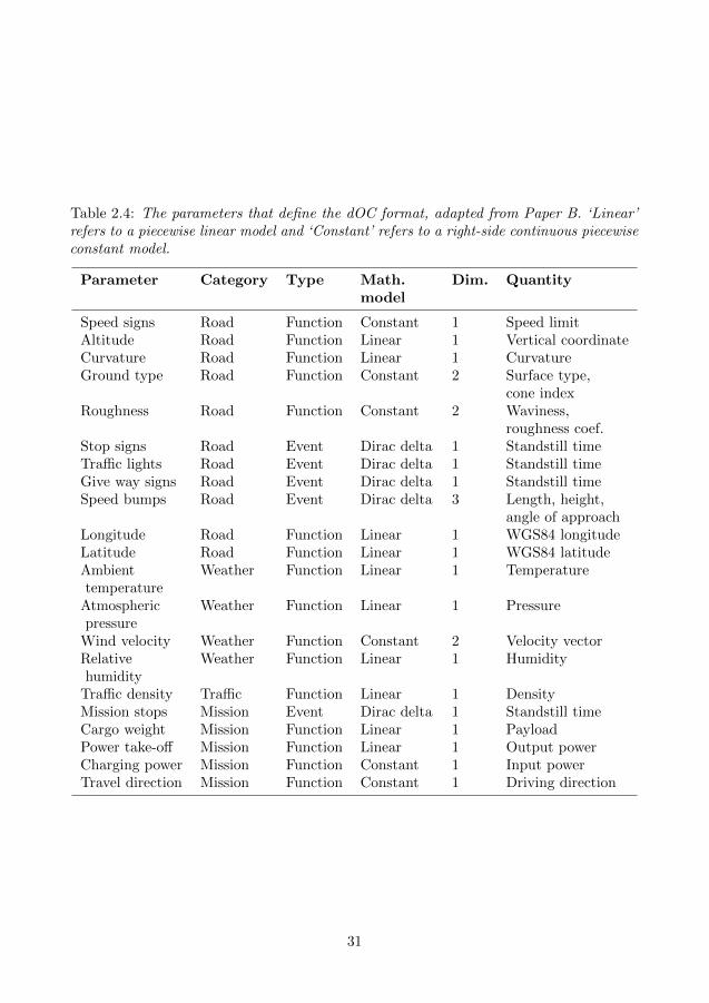
Table 2.4: The parameters that define the dOC format, adapted from Paper B. ‘Linear’refers to a piecewise linear model and ‘Constant’ refers to a right-side continuous piecewiseconstant model.

Parameter Category Type Math.model

Dim. Quantity

Speed signs Road Function Constant 1 Speed limitAltitude Road Function Linear 1 Vertical coordinateCurvature Road Function Linear 1 CurvatureGround type Road Function Constant 2 Surface type,

cone indexRoughness Road Function Constant 2 Waviness,

roughness coef.Stop signs Road Event Dirac delta 1 Standstill timeTraffic lights Road Event Dirac delta 1 Standstill timeGive way signs Road Event Dirac delta 1 Standstill timeSpeed bumps Road Event Dirac delta 3 Length, height,

angle of approachLongitude Road Function Linear 1 WGS84 longitudeLatitude Road Function Linear 1 WGS84 latitudeAmbienttemperature

Weather Function Linear 1 Temperature

Atmosphericpressure

Weather Function Linear 1 Pressure

Wind velocity Weather Function Constant 2 Velocity vectorRelativehumidity

Weather Function Linear 1 Humidity

Traffic density Traffic Function Linear 1 DensityMission stops Mission Event Dirac delta 1 Standstill timeCargo weight Mission Function Linear 1 PayloadPower take-off Mission Function Linear 1 Output powerCharging power Mission Function Constant 1 Input powerTravel direction Mission Function Constant 1 Driving direction

31

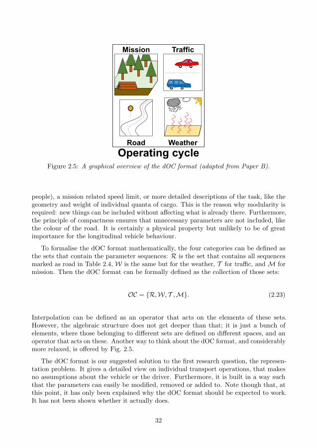
WeatherRoad

70

TrafficMission

Operating cycleFigure 2.5: A graphical overview of the dOC format (adapted from Paper B).

people), a mission related speed limit, or more detailed descriptions of the task, like thegeometry and weight of individual quanta of cargo. This is the reason why modularity isrequired: new things can be included without affecting what is already there. Furthermore,the principle of compactness ensures that unnecessary parameters are not included, likethe colour of the road. It is certainly a physical property but unlikely to be of greatimportance for the longitudinal vehicle behaviour.

To formalise the dOC format mathematically, the four categories can be defined asthe sets that contain the parameter sequences: R is the set that contains all sequencesmarked as road in Table 2.4, W is the same but for the weather, T for traffic, and M formission. Then the dOC format can be formally defined as the collection of those sets:

OC = {R,W, T ,M}. (2.23)

Interpolation can be defined as an operator that acts on the elements of these sets.However, the algebraic structure does not get deeper than that; it is just a bunch ofelements, where those belonging to different sets are defined on different spaces, and anoperator that acts on these. Another way to think about the dOC format, and considerablymore relaxed, is offered by Fig. 2.5.

The dOC format is our suggested solution to the first research question, the represen-tation problem. It gives a detailed view on individual transport operations, that makesno assumptions about the vehicle or the driver. Furthermore, it is built in a way suchthat the parameters can easily be modified, removed or added to. Note though that, atthis point, it has only been explained why the dOC format should be expected to work.It has not been shown whether it actually does.

32

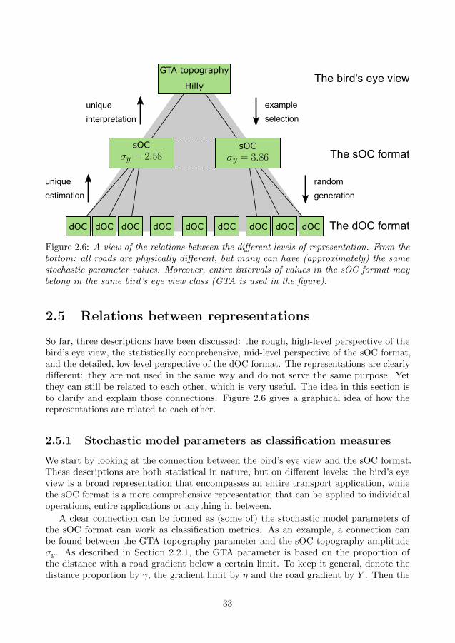
GTA topography

Hilly

dOC dOC dOC dOC dOC dOC dOC dOC dOC

sOC sOC

The bird's eye view

The sOC format

The dOC format

unique

interpretation

unique

estimation

random

generation

example

selection

Figure 2.6: A view of the relations between the different levels of representation. From thebottom: all roads are physically different, but many can have (approximately) the samestochastic parameter values. Moreover, entire intervals of values in the sOC format maybelong in the same bird’s eye view class (GTA is used in the figure).

2.5 Relations between representations

So far, three descriptions have been discussed: the rough, high-level perspective of thebird’s eye view, the statistically comprehensive, mid-level perspective of the sOC format,and the detailed, low-level perspective of the dOC format. The representations are clearlydifferent: they are not used in the same way and do not serve the same purpose. Yetthey can still be related to each other, which is very useful. The idea in this section isto clarify and explain those connections. Figure 2.6 gives a graphical idea of how therepresentations are related to each other.

2.5.1 Stochastic model parameters as classification measures

We start by looking at the connection between the bird’s eye view and the sOC format.These descriptions are both statistical in nature, but on different levels: the bird’s eyeview is a broad representation that encompasses an entire transport application, whilethe sOC format is a more comprehensive representation that can be applied to individualoperations, entire applications or anything in between.

A clear connection can be formed as (some of) the stochastic model parameters ofthe sOC format can work as classification metrics. As an example, a connection canbe found between the GTA topography parameter and the sOC topography amplitudeσy. As described in Section 2.2.1, the GTA parameter is based on the proportion ofthe distance with a road gradient below a certain limit. To keep it general, denote thedistance proportion by γ, the gradient limit by η and the road gradient by Y . Then the

33

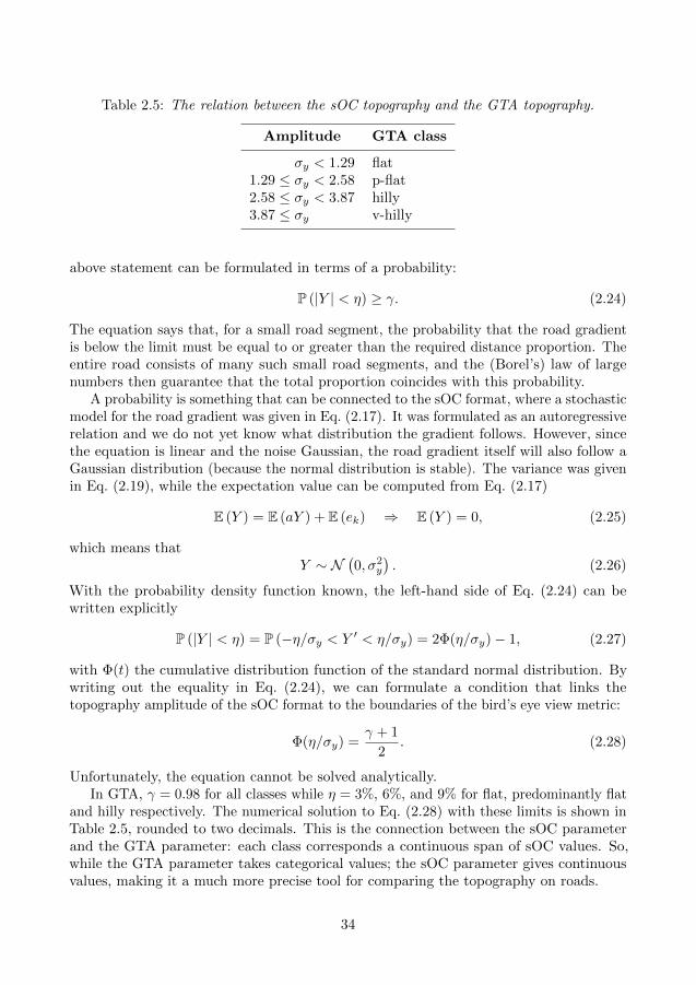
Table 2.5: The relation between the sOC topography and the GTA topography.

Amplitude GTA class

σy < 1.29 flat1.29 ≤ σy < 2.58 p-flat2.58 ≤ σy < 3.87 hilly3.87 ≤ σy v-hilly

above statement can be formulated in terms of a probability:

P (|Y | < η) ≥ γ. (2.24)

The equation says that, for a small road segment, the probability that the road gradientis below the limit must be equal to or greater than the required distance proportion. Theentire road consists of many such small road segments, and the (Borel’s) law of largenumbers then guarantee that the total proportion coincides with this probability.

A probability is something that can be connected to the sOC format, where a stochasticmodel for the road gradient was given in Eq. (2.17). It was formulated as an autoregressiverelation and we do not yet know what distribution the gradient follows. However, sincethe equation is linear and the noise Gaussian, the road gradient itself will also follow aGaussian distribution (because the normal distribution is stable). The variance was givenin Eq. (2.19), while the expectation value can be computed from Eq. (2.17)

E (Y ) = E (aY ) + E (ek) ⇒ E (Y ) = 0, (2.25)

which means thatY ∼ N

(0, σ2

y

). (2.26)

With the probability density function known, the left-hand side of Eq. (2.24) can bewritten explicitly

P (|Y | < η) = P (−η/σy < Y ′ < η/σy) = 2Φ(η/σy)− 1, (2.27)

with Φ(t) the cumulative distribution function of the standard normal distribution. Bywriting out the equality in Eq. (2.24), we can formulate a condition that links thetopography amplitude of the sOC format to the boundaries of the bird’s eye view metric:

Φ(η/σy) =γ + 1

2. (2.28)

Unfortunately, the equation cannot be solved analytically.In GTA, γ = 0.98 for all classes while η = 3%, 6%, and 9% for flat, predominantly flat

and hilly respectively. The numerical solution to Eq. (2.28) with these limits is shown inTable 2.5, rounded to two decimals. This is the connection between the sOC parameterand the GTA parameter: each class corresponds a continuous span of sOC values. So,while the GTA parameter takes categorical values; the sOC parameter gives continuousvalues, making it a much more precise tool for comparing the topography on roads.

34

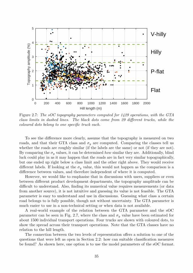
0 200 400 600 800 1000 1200 1400 1600 1800 2000

Hill length (m)

0

1

2

3

4

5T

opog

raph

y am

plitu

de (

%)

V-hilly

Hilly

P-flat

Flat

Figure 2.7: The sOC topography parameters computed for 1429 operations, with the GTAclass limits in dashed lines. The black dots come from 29 different trucks, while thecoloured dots belong to one specific truck each.

To see the difference more clearly, assume that the topography is measured on tworoads, and that their GTA class and σy are computed. Comparing the classes tell uswhether the roads are roughly similar (if the labels are the same) or not (if they are not).By comparing the σy values, it can be determined how similar they are. Additionally, blindluck could play in as it may happen that the roads are in fact very similar topographically,but one ended up right below a class limit and the other right above. They would receivedifferent labels. If looking at the σy value, this would not happen as the comparison is adifference between values, and therefore independent of where it is computed.

However, we would like to emphasise that in discussions with users, suppliers or evenbetween different product development departments, the topography amplitude can bedifficult to understand. Also, finding its numerical value requires measurements (or datafrom another source), it is not intuitive and guessing its value is not feasible. The GTAparameter is easy to understand and use in discussions. Guessing what class a certainroad belongs to is fully possible, though not without uncertainty. The GTA parameter ismuch easier to use in a non-technical setting or when data is not available.

A real-world example of the relation between the GTA parameter and the sOCparameter can be seen in Fig. 2.7, where the class and σy value have been estimated forabout 1500 individual transport operations. Four trucks are shown with coloured dots, toshow the spread across their transport operations. Note that the GTA classes have norelation to the hill length.

The connection between the two levels of representation offers a solution to one of thequestions that were left as open in Section 2.2: how can suitable classification measuresbe found? As shown here, one option is to use the model parameters of the sOC format.

35

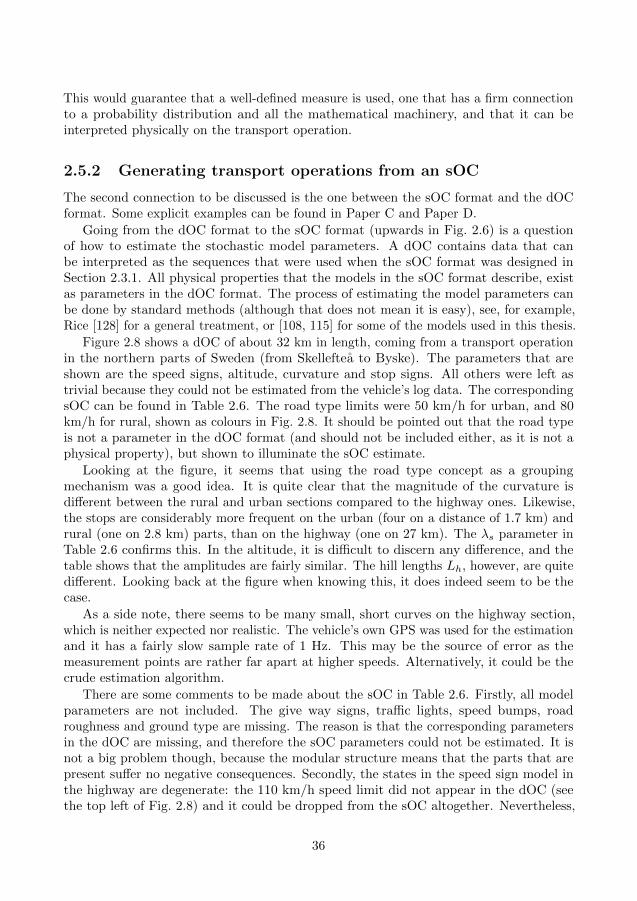
This would guarantee that a well-defined measure is used, one that has a firm connectionto a probability distribution and all the mathematical machinery, and that it can beinterpreted physically on the transport operation.

2.5.2 Generating transport operations from an sOC

The second connection to be discussed is the one between the sOC format and the dOCformat. Some explicit examples can be found in Paper C and Paper D.

Going from the dOC format to the sOC format (upwards in Fig. 2.6) is a questionof how to estimate the stochastic model parameters. A dOC contains data that canbe interpreted as the sequences that were used when the sOC format was designed inSection 2.3.1. All physical properties that the models in the sOC format describe, existas parameters in the dOC format. The process of estimating the model parameters canbe done by standard methods (although that does not mean it is easy), see, for example,Rice [128] for a general treatment, or [108, 115] for some of the models used in this thesis.

Figure 2.8 shows a dOC of about 32 km in length, coming from a transport operationin the northern parts of Sweden (from Skelleftea to Byske). The parameters that areshown are the speed signs, altitude, curvature and stop signs. All others were left astrivial because they could not be estimated from the vehicle’s log data. The correspondingsOC can be found in Table 2.6. The road type limits were 50 km/h for urban, and 80km/h for rural, shown as colours in Fig. 2.8. It should be pointed out that the road typeis not a parameter in the dOC format (and should not be included either, as it is not aphysical property), but shown to illuminate the sOC estimate.

Looking at the figure, it seems that using the road type concept as a groupingmechanism was a good idea. It is quite clear that the magnitude of the curvature isdifferent between the rural and urban sections compared to the highway ones. Likewise,the stops are considerably more frequent on the urban (four on a distance of 1.7 km) andrural (one on 2.8 km) parts, than on the highway (one on 27 km). The λs parameter inTable 2.6 confirms this. In the altitude, it is difficult to discern any difference, and thetable shows that the amplitudes are fairly similar. The hill lengths Lh, however, are quitedifferent. Looking back at the figure when knowing this, it does indeed seem to be thecase.

As a side note, there seems to be many small, short curves on the highway section,which is neither expected nor realistic. The vehicle’s own GPS was used for the estimationand it has a fairly slow sample rate of 1 Hz. This may be the source of error as themeasurement points are rather far apart at higher speeds. Alternatively, it could be thecrude estimation algorithm.

There are some comments to be made about the sOC in Table 2.6. Firstly, all modelparameters are not included. The give way signs, traffic lights, speed bumps, roadroughness and ground type are missing. The reason is that the corresponding parametersin the dOC are missing, and therefore the sOC parameters could not be estimated. It isnot a big problem though, because the modular structure means that the parts that arepresent suffer no negative consequences. Secondly, the states in the speed sign model inthe highway are degenerate: the 110 km/h speed limit did not appear in the dOC (seethe top left of Fig. 2.8) and it could be dropped from the sOC altogether. Nevertheless,

36

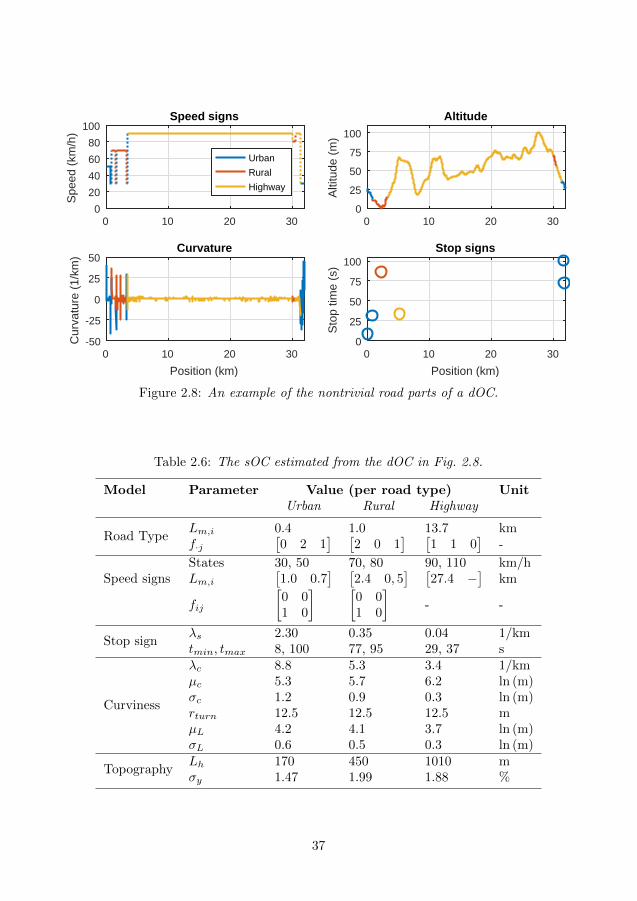
0 10 20 300

20

40

60

80

100

Spe

ed (

km/h

)

Speed signs

Urban

Rural

Highway

0 10 20 300

25

50

75

100

Alti

tude

(m

)

Altitude

0 10 20 30

Position (km)

-50

-25

0

25

50

Cur

vatu

re (

1/km

)

Curvature

0 10 20 30

Position (km)

0

25

50

75

100

Sto

p tim

e (s

)

Stop signs

Figure 2.8: An example of the nontrivial road parts of a dOC.

Table 2.6: The sOC estimated from the dOC in Fig. 2.8.

Model Parameter Value (per road type) UnitUrban Rural Highway

Road TypeLm,i 0.4 1.0 13.7 kmf·j

[0 2 1

] [2 0 1

] [1 1 0

]-

Speed signsStates 30, 50 70, 80 90, 110 km/hLm,i

[1.0 0.7

] [2.4 0, 5

] [27.4 −

]km

fij

[0 01 0

] [0 01 0

]- -

Stop signλs 2.30 0.35 0.04 1/kmtmin, tmax 8, 100 77, 95 29, 37 s

Curviness

λc 8.8 5.3 3.4 1/kmµc 5.3 5.7 6.2 ln (m)σc 1.2 0.9 0.3 ln (m)rturn 12.5 12.5 12.5 mµL 4.2 4.1 3.7 ln (m)σL 0.6 0.5 0.3 ln (m)

TopographyLh 170 450 1010 mσy 1.47 1.99 1.88 %

37

this is an explicit example of how to go from a dOC to an sOC.This connection makes it possible to characterise the sequences of the dOC parameters

in terms of the scalar model parameters of the sOC format: a classification with acontinuous metric. Comparing scalar values is trivial and therefore obviously muchsimpler to use when assessing similarities between operations, than the sequences in thedOC parameters are.

The connection in the other direction, from an sOC to a dOC, is theoretically easyyet can be of great practical use. Stochastic models are the building blocks of the sOCformat, meaning that new sequences can be created by generating random numbers5 fromthe respective probability distributions. The sequences that pop out are the same as thosein Section 2.3. Some of them are exactly the kind of ordered pair as the correspondingparameter in the dOC format, like the stop signs, while others need modification beforebecoming a valid member, like curviness to road curvature. The mathematical detailssurrounding the necessary conversion are given in Paper C.

Figure 2.9 shows two dOCs generated from the sOC in Table 2.6. The road typeis generated first (shown in colour), since it decides what values the other stochasticparameters take at all points. The grouping is seen in the curvature plot, as the curvescome out with different characteristics on the urban, rural and highway parts. Similarlyfor the stops. In the dOC on the left, there is only one stop, on a highway section, andthe reason is likely that only a very short urban section appeared: 380 m in length. Thismight seem odd, but given the urban stop intensity, the likelihood of this happening isabout 0.4, meaning that the event is nothing out of the ordinary.

Figure 2.9 is an example of the connection from an sOC to a dOC. While the resultsare not overly exciting, the practical implications that they have, are more so. The twogenerated dOCs are obviously different physically, as the two columns in Fig. 2.9 arenot identical. However, they originate from the same processes and distributions, whichmeans that they are statistically equivalent in this regard. Therefore, those dOCs canbe seen, together with the original one in Fig. 2.8, as different transport operations thatare set in the same kind of environment (the same landscape, in some sense): they arevariations of one another. In other words, given a transport operation, a dOC can beestimated first, and an sOC second (though it could be estimated straight from the datatoo). Then we can generate as many new dOCs as we want, all of which are variationsof the original. This is exactly what was asked for in the second half of the variationproblem: ‘how can variation be reproduced mathematically?’, to which we suggest thesolution: ‘by generating new operations from an sOC’.

5A probabilist or a statistician may refer to this as ‘simulation’ or ‘simulating random numbers’. Weuse ‘generation’ instead, to avoid confusion with the word simulation as used in the context of dynamicalsystems, where it means computational evolution of a system over time.

38

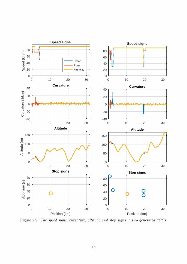
0 10 20 300

20

40

60

80

Speed signs

0 10 20 30-40

-20

0

20

40Curvature

0 10 20 300

50

100

150

Altitude

0 10 20 30

Position (km)

0

20

40

60

80

Stop signs

0 10 20 30-40

-20

0

20

40

Cur

vatu

re (

1/km

)

Curvature

0 10 20 300

50

100

150

Alti

tude

(m

)

Altitude

0 10 20 30

Position (km)

0

20

40

60

80

Sto

p tim

e (s

)

Stop signs

0 10 20 300

20

40

60

80

Spe

ed (

km/h

)

Speed signs

Urban

Rural

Highway

Figure 2.9: The speed signs, curvature, altitude and stop signs in two generated dOCs.

39

40

3 Modelling and simulation

The main topic of this section is the fourth research question, the simulation problem,the core of which is to conceptually explain how to build a dynamic model for simulationthat can use the data contained in a dOC. This is explained in some detail in Paper B,with additional information in [101]. Meanwhile, some basic modelling principles werelaid down in Paper A, which also contains the most sophisticated vehicle model, althoughthat may actually be the least interesting part from the thesis’ point of view. Paper Duses these ideas and compares two ways of approaching the simulation process but doesnot dig deeper into the functional modelling itself.

An in-depth description of the advanced vehicle model used in Paper A can be foundin [129]. In addition, vehicle modelling is a huge topic and there are many books thatintroduce the topic [35–41].

3.1 Model topology

To start out, we will have to discuss some principles that are needed in the virtualenvironment that is about to be constructed. These introduce requirements that lead towhat parts that the model must consist of at the very top level.

In the introduction, the need for realism in a virtual environment was argued, toincrease the chance that the developed products work as predicted. This was the reasonwhy the dOC format was designed. To use road data (and other data) given on such aform, a corresponding dynamic model of the operating cycle (OC) must be constructed.A dynamic model of the vehicle is also necessary, since this is the system under test foran original equipment manufacturer. However, these two parts alone are not enough.Unlike the target speed in a conventional driving cycle, the data in the dOC does notstipulate how a vehicle should move. It does provide the speed limit, which is the (legal)upper bound, but there are many situations where it does not make sense to keep this:in curves, around bumps, on rough ground, on slippery surfaces, around other vehicles,and more. In reality, there is a driver inside the vehicle who reacts to the situation onthe road and controls the vehicle to the best of his or her ability. As long as the vehicleis not fully automated, some kind of driver model is needed. The more automated thevehicle becomes, the simpler the driver model can be and the more extensive the flow ofinformation from OC to vehicle has to be.

With these three models in mind: the OC, the driver and the vehicle, a fair ideaof how the environment could look at the top level was already provided by Fig. 1.4.The three models have no components in common but share information through theirinterfaces. A modular structure like this is advantageous, because a component can beswitched out (or just the data inside it) without affecting the others. This is convenientin practice, because then the, say, vehicle can be replaced while the driver and OC remainthe same. That is precisely what one would want if trying to find the best vehicle designfor a particular transport operation and driver, for an entire transport application, or fora class of drivers.

The interfaces between the models should correspond to their physical counterparts in

41

the real world. For a given position, the forces on the vehicle are decided by the propertiesof the road through the contacts with the ground and air as taught by the basic laws ofphysics, as in Fig. 2.1. The interface between the driver and the road is the optical flow:the driver can see, for example, the road’s signs and signals, its geometry and the surfacecondition. This gives the person information both about the moment and some distanceahead, depending on what the visibility is like. The interface between the driver and thevehicle are the actuators: the accelerator and brake pedals, the steering wheel, possibly agear stick, and various buttons, like cruise control activation. Sensor information, like thespeedometer, is also available.

With these principles in mind, we can start discussing individual models for the OC,the driver and the vehicle.

3.1.1 An operating cycle model

The first model to be discussed is that of the OC. Note the difference between the dynamicmodel and the dOC format itself. A dOC contains static data, and the idea is to build adynamic model that can be parametrised by such data (meaning that the model takes thedata as input before any simulation starts and keeps it constant), to work together withthe driver and vehicle models. The dynamic OC model sends out the current value of thephysical quantities in the data based on the position of the vehicle, and some upcomingvalues depending on how far the driver can see.

The purpose of the model is to provide a value for all dOC parameters at any giventime instant during the simulation. The road category contains physical parameters thatdescribes the trajectory, signs and signals. These only vary by position, so one input tothe OC model must be the position of the vehicle x along the trajectory, measured atsome convenient reference point, like the centre of mass, the front bumper, or the frontaxle. The weather, traffic and mission categories can obviously change with positiontoo, but they may also have an explicit time dependence, for example: when using amounted crane to load or unload cargo. Thus, the current time t must also be an input.In addition, the vehicle speed v will be needed, not for the parameters themselves but forpurely technical reasons: to separate between a vehicle at standstill and at motion.

A stylised idea of what an implementation may look like is shown in Fig. 3.1. Here,each category in the dOC format has its own module, to adhere to the principle ofmodularity. The road, traffic and weather modules are uncomplicated; each parameter phas an underlying (suggested) mathematical model fp(x, xi, . . . , pi, . . . ), listed in Table 2.4.Then it is only a problem of interpolation to find the value of p at any position x betweenthe points (xi, pi) and (xi+1, pi+1) where its value is tabulated:

i : xi ≤ x < xi+1, (3.1)

p = fp (x, xi, xi+1, pi, pi+1) . (3.2)

Interpolation in time works equivalently.The mission module is more complicated because it can be active both when moving

and during standstill, and it needs to consider which variable that governs the simulation.Of course, time is always an independent variable in a dynamic simulation. However,when the vehicle is moving, the explicit dependence in Eqs. (3.1) and (3.2) is position

42

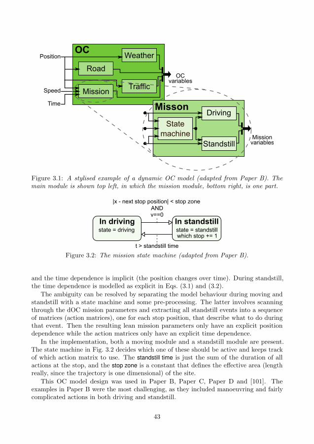
Weather

Mission

Road

Position

Speed

Time

OC

Misson

Statemachine

Traffic

OCvariables

Missionvariables

Driving

Standstill

Figure 3.1: A stylised example of a dynamic OC model (adapted from Paper B). Themain module is shown top left, in which the mission module, bottom right, is one part.

v==0

|x - next stop position| < stop zone

t > standstill time

AND

In standstillstate = standstillwhich stop += 1

In drivingstate = driving

Figure 3.2: The mission state machine (adapted from Paper B).

and the time dependence is implicit (the position changes over time). During standstill,the time dependence is modelled as explicit in Eqs. (3.1) and (3.2).

The ambiguity can be resolved by separating the model behaviour during moving andstandstill with a state machine and some pre-processing. The latter involves scanningthrough the dOC mission parameters and extracting all standstill events into a sequenceof matrices (action matrices), one for each stop position, that describe what to do duringthat event. Then the resulting lean mission parameters only have an explicit positiondependence while the action matrices only have an explicit time dependence.

In the implementation, both a moving module and a standstill module are present.The state machine in Fig. 3.2 decides which one of these should be active and keeps trackof which action matrix to use. The standstill time is just the sum of the duration of allactions at the stop, and the stop zone is a constant that defines the effective area (lengthreally, since the trajectory is one dimensional) of the site.

This OC model design was used in Paper B, Paper C, Paper D and [101]. Theexamples in Paper B were the most challenging, as they included manoeuvring and fairlycomplicated actions in both driving and standstill.

43

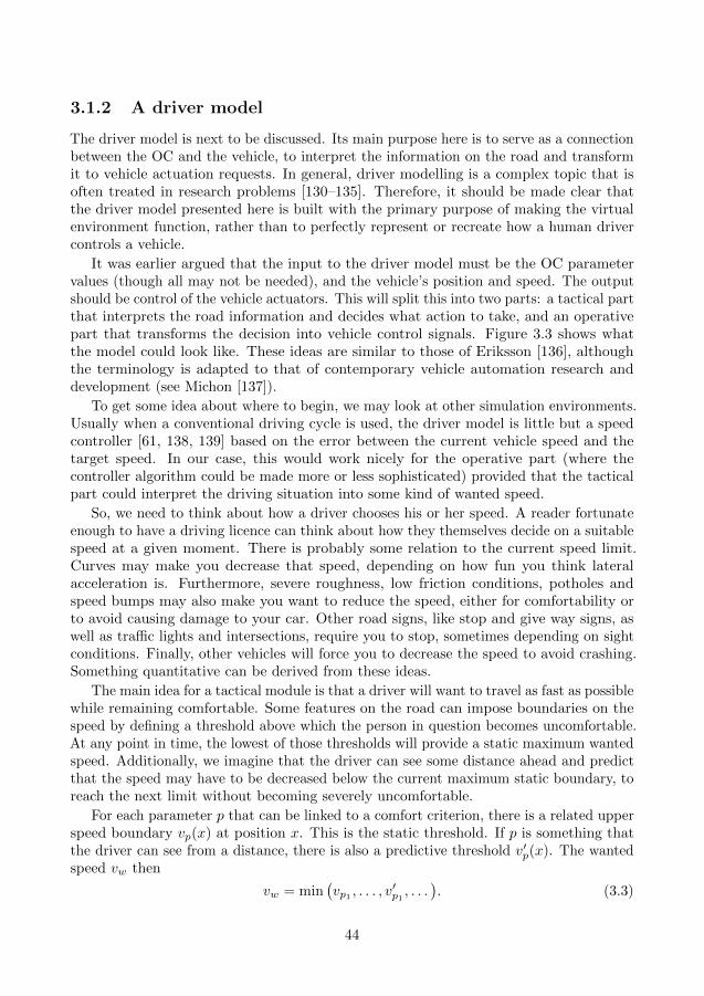
3.1.2 A driver model

The driver model is next to be discussed. Its main purpose here is to serve as a connectionbetween the OC and the vehicle, to interpret the information on the road and transformit to vehicle actuation requests. In general, driver modelling is a complex topic that isoften treated in research problems [130–135]. Therefore, it should be made clear thatthe driver model presented here is built with the primary purpose of making the virtualenvironment function, rather than to perfectly represent or recreate how a human drivercontrols a vehicle.

It was earlier argued that the input to the driver model must be the OC parametervalues (though all may not be needed), and the vehicle’s position and speed. The outputshould be control of the vehicle actuators. This will split this into two parts: a tactical partthat interprets the road information and decides what action to take, and an operativepart that transforms the decision into vehicle control signals. Figure 3.3 shows whatthe model could look like. These ideas are similar to those of Eriksson [136], althoughthe terminology is adapted to that of contemporary vehicle automation research anddevelopment (see Michon [137]).

To get some idea about where to begin, we may look at other simulation environments.Usually when a conventional driving cycle is used, the driver model is little but a speedcontroller [61, 138, 139] based on the error between the current vehicle speed and thetarget speed. In our case, this would work nicely for the operative part (where thecontroller algorithm could be made more or less sophisticated) provided that the tacticalpart could interpret the driving situation into some kind of wanted speed.

So, we need to think about how a driver chooses his or her speed. A reader fortunateenough to have a driving licence can think about how they themselves decide on a suitablespeed at a given moment. There is probably some relation to the current speed limit.Curves may make you decrease that speed, depending on how fun you think lateralacceleration is. Furthermore, severe roughness, low friction conditions, potholes andspeed bumps may also make you want to reduce the speed, either for comfortability orto avoid causing damage to your car. Other road signs, like stop and give way signs, aswell as traffic lights and intersections, require you to stop, sometimes depending on sightconditions. Finally, other vehicles will force you to decrease the speed to avoid crashing.Something quantitative can be derived from these ideas.

The main idea for a tactical module is that a driver will want to travel as fast as possiblewhile remaining comfortable. Some features on the road can impose boundaries on thespeed by defining a threshold above which the person in question becomes uncomfortable.At any point in time, the lowest of those thresholds will provide a static maximum wantedspeed. Additionally, we imagine that the driver can see some distance ahead and predictthat the speed may have to be decreased below the current maximum static boundary, toreach the next limit without becoming severely uncomfortable.

For each parameter p that can be linked to a comfort criterion, there is a related upperspeed boundary vp(x) at position x. This is the static threshold. If p is something thatthe driver can see from a distance, there is also a predictive threshold v′p(x). The wantedspeed vw then

vw = min(vp1

, . . . , v′p1, . . .

). (3.3)

44

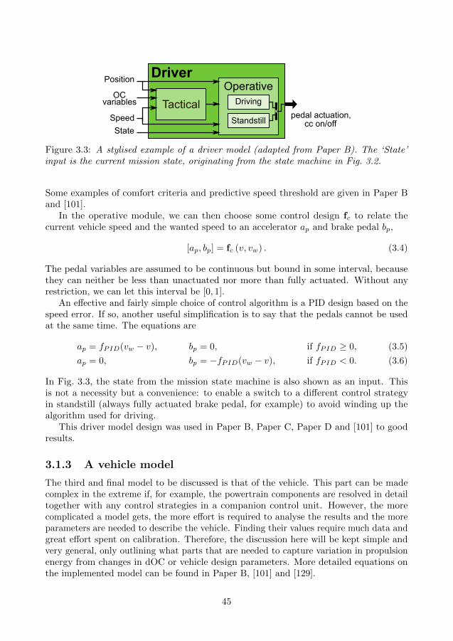
Driver

Tactical

OperativePosition

Speed

OCvariables

pedal actuation,cc on/offStandstill

Driving

State

Figure 3.3: A stylised example of a driver model (adapted from Paper B). The ‘State’input is the current mission state, originating from the state machine in Fig. 3.2.

Some examples of comfort criteria and predictive speed threshold are given in Paper Band [101].

In the operative module, we can then choose some control design fc to relate thecurrent vehicle speed and the wanted speed to an accelerator ap and brake pedal bp,

[ap, bp] = fc (v, vw) . (3.4)

The pedal variables are assumed to be continuous but bound in some interval, becausethey can neither be less than unactuated nor more than fully actuated. Without anyrestriction, we can let this interval be [0, 1].

An effective and fairly simple choice of control algorithm is a PID design based on thespeed error. If so, another useful simplification is to say that the pedals cannot be usedat the same time. The equations are

ap = fPID(vw − v), bp = 0, if fPID ≥ 0, (3.5)

ap = 0, bp = −fPID(vw − v), if fPID < 0. (3.6)

In Fig. 3.3, the state from the mission state machine is also shown as an input. Thisis not a necessity but a convenience: to enable a switch to a different control strategyin standstill (always fully actuated brake pedal, for example) to avoid winding up thealgorithm used for driving.

This driver model design was used in Paper B, Paper C, Paper D and [101] to goodresults.

3.1.3 A vehicle model

The third and final model to be discussed is that of the vehicle. This part can be madecomplex in the extreme if, for example, the powertrain components are resolved in detailtogether with any control strategies in a companion control unit. However, the morecomplicated a model gets, the more effort is required to analyse the results and the moreparameters are needed to describe the vehicle. Finding their values require much data andgreat effort spent on calibration. Therefore, the discussion here will be kept simple andvery general, only outlining what parts that are needed to capture variation in propulsionenergy from changes in dOC or vehicle design parameters. More detailed equations onthe implemented model can be found in Paper B, [101] and [129].

45

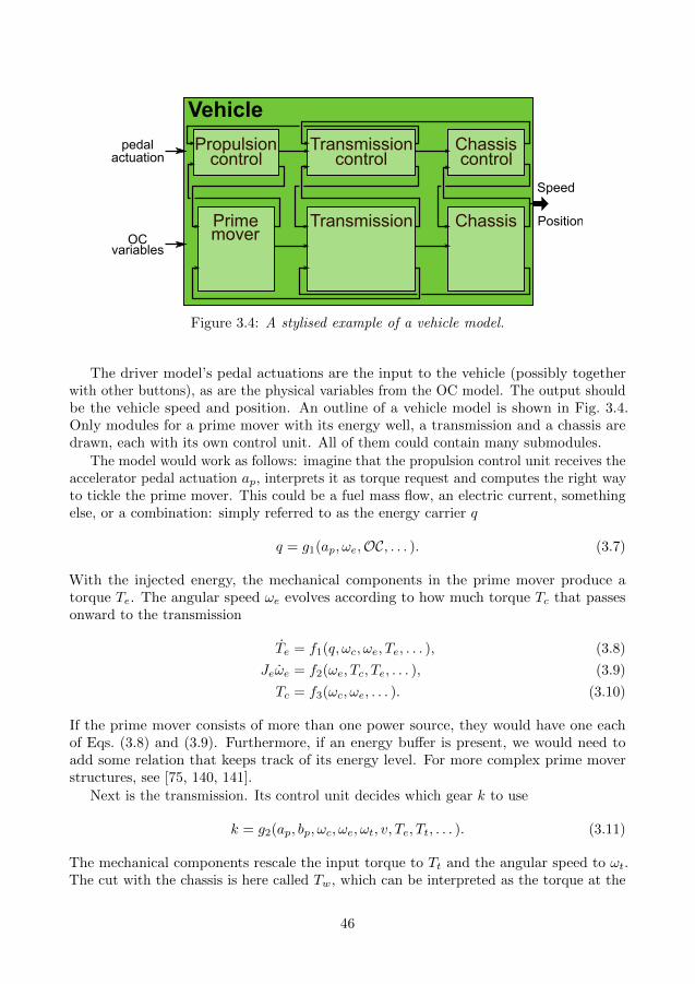
Vehicle

Speed

OCvariables

Primemover

Transmission Chassis

Propulsioncontrol

Transmissioncontrol

Chassiscontrol

Position

pedalactuation

Figure 3.4: A stylised example of a vehicle model.

The driver model’s pedal actuations are the input to the vehicle (possibly togetherwith other buttons), as are the physical variables from the OC model. The output shouldbe the vehicle speed and position. An outline of a vehicle model is shown in Fig. 3.4.Only modules for a prime mover with its energy well, a transmission and a chassis aredrawn, each with its own control unit. All of them could contain many submodules.

The model would work as follows: imagine that the propulsion control unit receives theaccelerator pedal actuation ap, interprets it as torque request and computes the right wayto tickle the prime mover. This could be a fuel mass flow, an electric current, somethingelse, or a combination: simply referred to as the energy carrier q

q = g1(ap, ωe,OC, . . . ). (3.7)

With the injected energy, the mechanical components in the prime mover produce atorque Te. The angular speed ωe evolves according to how much torque Tc that passesonward to the transmission

Te = f1(q, ωc, ωe, Te, . . . ), (3.8)

Jeωe = f2(ωe, Tc, Te, . . . ), (3.9)

Tc = f3(ωc, ωe, . . . ). (3.10)

If the prime mover consists of more than one power source, they would have one eachof Eqs. (3.8) and (3.9). Furthermore, if an energy buffer is present, we would need toadd some relation that keeps track of its energy level. For more complex prime moverstructures, see [75, 140, 141].

Next is the transmission. Its control unit decides which gear k to use

k = g2(ap, bp, ωc, ωe, ωt, v, Te, Tt, . . . ). (3.11)

The mechanical components rescale the input torque to Tt and the angular speed to ωt.The cut with the chassis is here called Tw, which can be interpreted as the torque at the

46

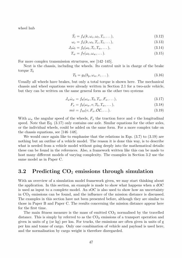
wheel hub

Tt = f4(k, ωc, ωt, Tc, . . . ), (3.12)

ωc = f5(k, ωt, Tc, Tt, . . . ), (3.13)

Jtωt = f6(ωt, Tt, Tw, . . . ), (3.14)

Tw = f7(ωt, ωw, . . . ). (3.15)

For more complex transmission structures, see [142–145].Next is the chassis, including the wheels. Its control unit is in charge of the brake

torque TbTb = g3(bp, ωw, v, . . . ). (3.16)

Usually all wheels have brakes, but only a total torque is shown here. The mechanicalchassis and wheel equations were already written in Section 2.1 for a two-axle vehicle,but they can be written on the same general form as the other two systems

Jwωw = f8(ωw, Tb, Tw, Fx, . . . ), (3.17)

Fx = f9(ωw, v, Tb, Tw, . . . ), (3.18)

mv = f10(v, Fx,OC, . . . ). (3.19)

With ωw the angular speed of the wheels, Fx the traction force and v the longitudinalspeed. Note that Eq. (3.17) only contains one axle. Similar equations for the other axles,or the individual wheels, could be added on the same form. For a more complex take onthe chassis equations, see [146–148].

We would once again like to emphasise that the relations in Eqs. (3.7) to (3.19) arenothing but an outline of a vehicle model. The reason it is done this way, is to describewhat is needed from a vehicle model without going deeply into the mathematical details:these can be found in the references. Also, a framework written like this can be made tohost many different models of varying complexity. The examples in Section 3.2 use thesame model as in Paper C.

3.2 Predicting CO2 emissions through simulation

With an overview of a simulation model framework given, we may start thinking aboutthe application. In this section, an example is made to show what happens when a dOCis used as input to a complete model. An sOC is also used to show how an uncertaintyin CO2 emissions can be found, and the influence of the mission distance is discussed.The examples in this section have not been presented before, although they are similar tothose in Paper B and Paper C. The results concerning the mission distance appear herefor the first time.

The main fitness measure is the mass of emitted CO2 normalised by the travelleddistance. This is simply by referred to as the CO2 emissions of a transport operation andgiven in units of g (or kg) per km. For trucks, the emissions are often given in units of gper km and tonne of cargo. Only one combination of vehicle and payload is used here,and the normalisation by cargo weight is therefore disregarded.

47

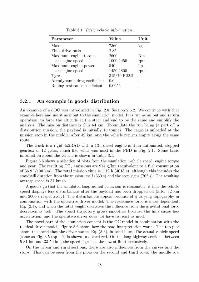
Table 3.1: Basic vehicle information.

Parameter Value Unit

Mass 7360 kgFinal drive ratio 2.85 -Maximum engine torque 2600 Nm

at engine speed 1000-1450 rpmMaximum engine power 540 hp

at engine speed 1450-1800 rpmTyres 315/70 R22.5 -Aerodynamic drag coefficient 0.6 -Rolling resistance coefficient 0.0056 -

3.2.1 An example in goods distribution

An example of a dOC was introduced in Fig. 2.8, Section 2.5.2. We continue with thatexample here and use it as input to the simulation model. It is run as an out and returnoperation, to force the altitude at the start and end to be the same and simplify theanalysis. The mission distance is thus 64 km. To emulate the run being (a part of) adistribution mission, the payload is initially 15 tonnes. The cargo is unloaded at themission stop in the middle, after 32 km, and the vehicle returns empty along the sameroute.

The truck is a rigid 4x2RAD with a 13 l diesel engine and an automated, steppedgearbox of 12 gears, much like what was used in the FBD in Fig. 2.1. Some basicinformation about the vehicle is shown in Table 3.1.

Figure 3.5 shows a selection of plots from the simulation: vehicle speed, engine torqueand gear. The resulting CO2 emissions are 974 g/km (equivalent to a fuel consumptionof 36.9 l/100 km). The total mission time is 1.12 h (4018 s), although this includes thestandstill duration from the mission itself (330 s) and the stop signs (702 s). The resultingaverage speed is 57 km/h.

A good sign that the simulated longitudinal behaviour is reasonable, is that the vehiclespeed displays less disturbances after the payload has been dropped off (after 32 kmand 2000 s respectively). The disturbances appear because of a varying topography incombination with the operative driver model. The resistance force is mass dependent,Eq. (2.1), and when the total weight decreases the influence from the gravitational forcedecreases as well. The speed trajectory grows smoother because the hills cause lessacceleration, and the operative driver does not have to react as much.

The novel part of the simulation concept is the OC model in combination with thetactical driver model. Figure 3.6 shows how the road interpretation works. The top plotshows the speed that the driver wants, Eq. (3.3), in solid blue. The actual vehicle speed(same as Fig. 3.5 top left) is shown in dotted red. On the long highway sections, between5-31 km and 33-59 km, the speed signs set the lowest limit exclusively.

On the urban and rural sections, there are also influences from the curves and thestops. This can be seen from the plots on the second and third rows: the middle row

48

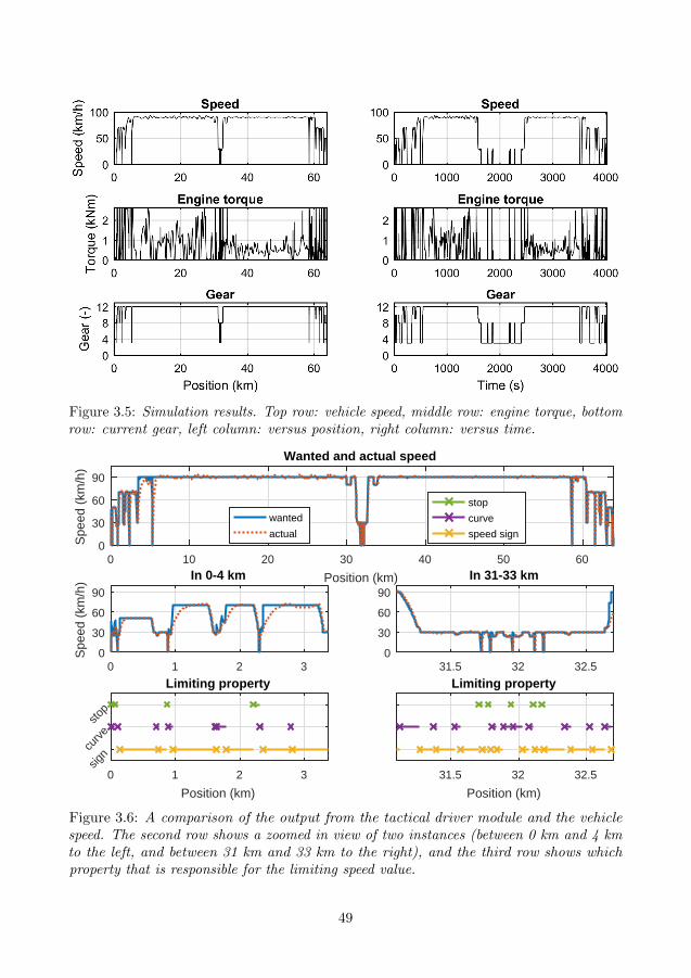
Figure 3.5: Simulation results. Top row: vehicle speed, middle row: engine torque, bottomrow: current gear, left column: versus position, right column: versus time.

0 10 20 30 40 50 60

Position (km)

0

30

60

90

Spe

ed (

km/h

)

Wanted and actual speed

wanted

actual

0 1 2 30

30

60

90

Spe

ed (

km/h

) In 0-4 km

31.5 32 32.50

30

60

90

In 31-33 km

stop

curve

speed sign

0 1 2 3

Position (km)

sign

curv

esto

p

Limiting property

31.5 32 32.5

Position (km)

Limiting property

Figure 3.6: A comparison of the output from the tactical driver module and the vehiclespeed. The second row shows a zoomed in view of two instances (between 0 km and 4 kmto the left, and between 31 km and 33 km to the right), and the third row shows whichproperty that is responsible for the limiting speed value.

49

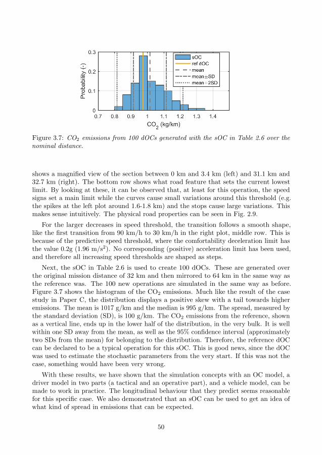
Figure 3.7: CO2 emissions from 100 dOCs generated with the sOC in Table 2.6 over thenominal distance.

shows a magnified view of the section between 0 km and 3.4 km (left) and 31.1 km and32.7 km (right). The bottom row shows what road feature that sets the current lowestlimit. By looking at these, it can be observed that, at least for this operation, the speedsigns set a main limit while the curves cause small variations around this threshold (e.g.the spikes at the left plot around 1.6-1.8 km) and the stops cause large variations. Thismakes sense intuitively. The physical road properties can be seen in Fig. 2.9.

For the larger decreases in speed threshold, the transition follows a smooth shape,like the first transition from 90 km/h to 30 km/h in the right plot, middle row. This isbecause of the predictive speed threshold, where the comfortability deceleration limit hasthe value 0.2g (1.96 m/s2). No corresponding (positive) acceleration limit has been used,and therefore all increasing speed thresholds are shaped as steps.

Next, the sOC in Table 2.6 is used to create 100 dOCs. These are generated overthe original mission distance of 32 km and then mirrored to 64 km in the same way asthe reference was. The 100 new operations are simulated in the same way as before.Figure 3.7 shows the histogram of the CO2 emissions. Much like the result of the casestudy in Paper C, the distribution displays a positive skew with a tail towards higheremissions. The mean is 1017 g/km and the median is 995 g/km. The spread, measured bythe standard deviation (SD), is 100 g/km. The CO2 emissions from the reference, shownas a vertical line, ends up in the lower half of the distribution, in the very bulk. It is wellwithin one SD away from the mean, as well as the 95% confidence interval (approximatelytwo SDs from the mean) for belonging to the distribution. Therefore, the reference dOCcan be declared to be a typical operation for this sOC. This is good news, since the dOCwas used to estimate the stochastic parameters from the very start. If this was not thecase, something would have been very wrong.

With these results, we have shown that the simulation concepts with an OC model, adriver model in two parts (a tactical and an operative part), and a vehicle model, can bemade to work in practice. The longitudinal behaviour that they predict seems reasonablefor this specific case. We also demonstrated that an sOC can be used to get an idea ofwhat kind of spread in emissions that can be expected.

50

3.2.2 About expected consumption, variance and mission length

The CO2 emissions are one measure of a vehicle’s energy efficiency, the used mass perdistance. Fuel consumption is another. One could even be more general and define ‘energyusage’ as the required input energy per distance unit, to remove any dependence on whatmedium said energy comes from. Whichever one of these are used, an sOC could be usedto predict a mean and a spread. However, the mission distance has a curious effect onthese. To see it, consider the following situation, where the fuel consumption is used asthe canonical example.

Let’s assume that we have been given an sOC, generated a bunch of dOCs over a missiondistance L and simulated these. Both the total fuel mass m and the fuel consumptionf can be computed for each operation. These form some distribution (unknown which)and a mean mass m and variance σ2

m can be computed, likewise a mean consumption fand variance σ2

f . If we then treat the fuel mass as coming from a sequence of randomvariables {Mk}, we can write down a stochastic model as just a random value that variesaround a mean

Mk = m+ ek, E (ek) = 0, Var (ek) = σ2m, (3.20)

although we have absolutely no idea what distribution the error term ek follows. Thestochastic fuel consumption {Fk} is then the above normalised by the distance

Fk =Mk

L= f + εk, (3.21)

where

E (Fk) = f =m

L, Var (Fk) =

σ2m

L2= σ2

f . (3.22)

Now let’s say that we double the mission distance L′ = 2L but otherwise keep the sOCparameters unchanged: what happens to the mean and variance of the fuel consumption?The landscape is the same, which means that the vehicle would behave similarly. Wecan formulate a stochastic model for the new fuel mass {M ′k} by using the old one inEq. (3.20): for twice the distance we would just need to pick two of the original dOCsand put them together, one after the other. For ease of notation, drop the k-index in theanalysis

M ′ = M1 +M2 = 2m+ e1 + e2. (3.23)

The new expected value and variance then

E (M ′) = 2m, Var (M ′) = Var (e1 + e2) = 2σ2m, (3.24)

where the last equality comes about because the errors are uncorrelated,

Cov (e1, e2) = 0, (3.25)

since the landscape is statistically equivalent on both halves of the new operation. Thenew fuel consumption F′ would be

F′ =M ′

L′=M ′

2L, (3.26)

51

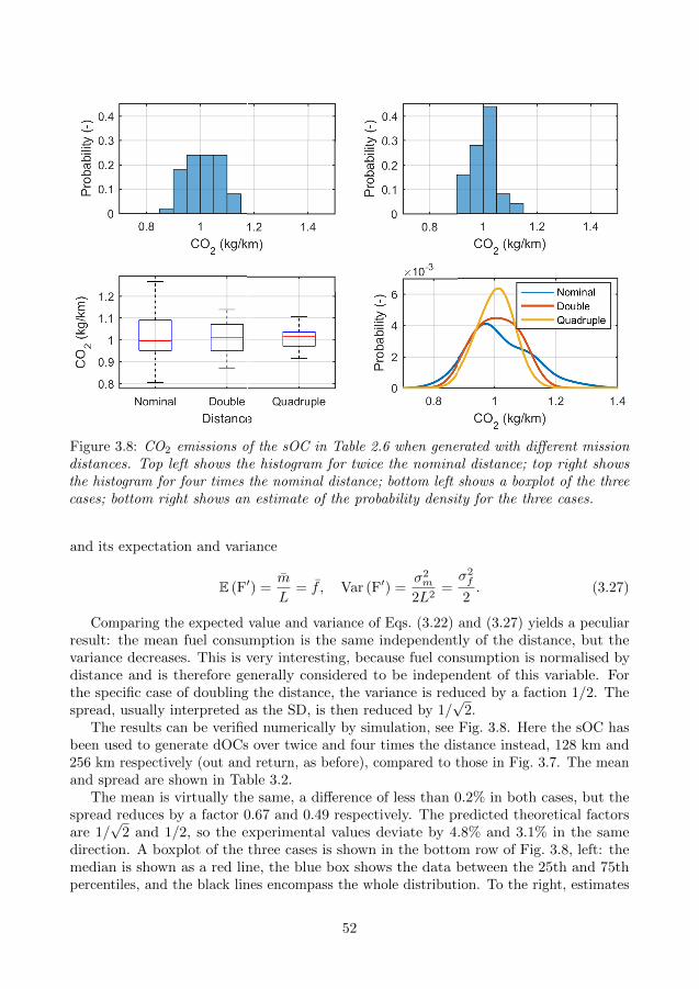
Figure 3.8: CO2 emissions of the sOC in Table 2.6 when generated with different missiondistances. Top left shows the histogram for twice the nominal distance; top right showsthe histogram for four times the nominal distance; bottom left shows a boxplot of the threecases; bottom right shows an estimate of the probability density for the three cases.

and its expectation and variance

E (F′) =m

L= f , Var (F′) =

σ2m

2L2=σ2f

2. (3.27)

Comparing the expected value and variance of Eqs. (3.22) and (3.27) yields a peculiarresult: the mean fuel consumption is the same independently of the distance, but thevariance decreases. This is very interesting, because fuel consumption is normalised bydistance and is therefore generally considered to be independent of this variable. Forthe specific case of doubling the distance, the variance is reduced by a faction 1/2. Thespread, usually interpreted as the SD, is then reduced by 1/

√2.

The results can be verified numerically by simulation, see Fig. 3.8. Here the sOC hasbeen used to generate dOCs over twice and four times the distance instead, 128 km and256 km respectively (out and return, as before), compared to those in Fig. 3.7. The meanand spread are shown in Table 3.2.

The mean is virtually the same, a difference of less than 0.2% in both cases, but thespread reduces by a factor 0.67 and 0.49 respectively. The predicted theoretical factorsare 1/

√2 and 1/2, so the experimental values deviate by 4.8% and 3.1% in the same

direction. A boxplot of the three cases is shown in the bottom row of Fig. 3.8, left: themedian is shown as a red line, the blue box shows the data between the 25th and 75thpercentiles, and the black lines encompass the whole distribution. To the right, estimates

52

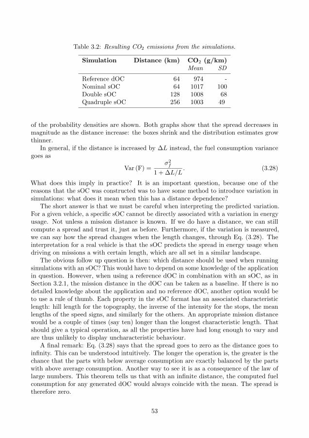
Table 3.2: Resulting CO2 emissions from the simulations.

Simulation Distance (km) CO2 (g/km)Mean SD

Reference dOC 64 974 -Nominal sOC 64 1017 100Double sOC 128 1008 68Quadruple sOC 256 1003 49

of the probability densities are shown. Both graphs show that the spread decreases inmagnitude as the distance increase: the boxes shrink and the distribution estimates growthinner.

In general, if the distance is increased by ∆L instead, the fuel consumption variancegoes as

Var (F) =σ2f

1 + ∆L/L. (3.28)

What does this imply in practice? It is an important question, because one of thereasons that the sOC was constructed was to have some method to introduce variation insimulations: what does it mean when this has a distance dependence?

The short answer is that we must be careful when interpreting the predicted variation.For a given vehicle, a specific sOC cannot be directly associated with a variation in energyusage. Not unless a mission distance is known. If we do have a distance, we can stillcompute a spread and trust it, just as before. Furthermore, if the variation is measured,we can say how the spread changes when the length changes, through Eq. (3.28). Theinterpretation for a real vehicle is that the sOC predicts the spread in energy usage whendriving on missions a with certain length, which are all set in a similar landscape.

The obvious follow up question is then: which distance should be used when runningsimulations with an sOC? This would have to depend on some knowledge of the applicationin question. However, when using a reference dOC in combination with an sOC, as inSection 3.2.1, the mission distance in the dOC can be taken as a baseline. If there is nodetailed knowledge about the application and no reference dOC, another option would beto use a rule of thumb. Each property in the sOC format has an associated characteristiclength: hill length for the topography, the inverse of the intensity for the stops, the meanlengths of the speed signs, and similarly for the others. An appropriate mission distancewould be a couple of times (say ten) longer than the longest characteristic length. Thatshould give a typical operation, as all the properties have had long enough to vary andare thus unlikely to display uncharacteristic behaviour.

A final remark: Eq. (3.28) says that the spread goes to zero as the distance goes toinfinity. This can be understood intuitively. The longer the operation is, the greater is thechance that the parts with below average consumption are exactly balanced by the partswith above average consumption. Another way to see it is as a consequence of the law oflarge numbers. This theorem tells us that with an infinite distance, the computed fuelconsumption for any generated dOC would always coincide with the mean. The spread istherefore zero.

53

54

4 Discussion, conclusion and outlook

In this chapter, we will summarise what has been done in the thesis. We will also saysomething about what has not been done, by giving an outlook on possible ways tocontinue.

4.1 Discussion and conclusion

We return to the research questions posed in the introduction

I. The representation problem: how should a transport operation be describedmathematically to enable a realistic vehicle usage?

II. The classification problem: how can transport applications be compared, withrespect to geographical and operational features, in a way that is both vehicle anddriver independent?

III. The variation problem: how can variation in operation be measured for transportoperations, and how can it be reproduced mathematically?

IV. The simulation problem: how should a complete model for dynamic simulationsbe built to use the detailed mathematical representation of a transport operation,and are there any basic principles it should follow?

Questions I-III were all discussed in Chapter 2, while question IV was the topic ofChapter 3.

In Chapter 2 three kinds of representations were presented. We started by motivatingwhat aspects of the transport operation that should be considered when talking aboutenergy usage. These were sorted into four categories: the road, the weather, the trafficand the mission.

Next, the classification problem was discussed in conjunction with the first representa-tion: the bird’s eye view. This was defined as a highly generalised description that onlygave a rough outline of an entire transport application, sparse with details. The missiondistance was used as an example to construct a classification parameter with three classes.The framework used by a vehicle manufacturer (Volvo trucks used as an example), theglobal transport application (GTA), was mentioned as an existing classification system.Three of its parameters were disseminated as to how they were defined, their metric andtheir classes.

The bird’s eye view representation is our suggested solution to the second researchquestion. It is a solution that leaves much to be desired though, because an explicitclassification parameter was only given for a single operational property. Furthermore,an ad hoc method was used to find the metric and the classes, but a more scientific wayshould be possible. Therefore, while the question of how to make comparisons betweentransport applications may have been solved in theory, it was not solved in practice.Three new questions appeared during the construction of the classification parameter:‘how can a metric be chosen in a scientific way?’; ‘how can it be verified that the choice

55

is sound?’; and ‘how can the classification limits be chosen systematically?’. A possiblesolution to the first of these new questions was found later: the sOC parameters. Thenthe second question is automatically answered too, by the arguments that were used tomotivate the stochastic processes in the first place. The last question, however, remainsto be answered.

The second representation that was discussed, in connection with the variation problem,was the stochastic operating cycle (sOC) format. This was a comprehensive yet abstractdescription that could treat transport operations individually or in a collection. It wassaid to have an intermediate level of detail, because of the one-to-many correspondencewith physical roads: each road on the planet corresponded uniquely to one sOC, but agiven sOC could describe many roads. The road properties were treated as sequencesof random numbers and then modelled individually by a stochastic process, dependingon how each sequence behaved. The parameters of those models had a firm statisticalbackground as they were related to the probability distributions that modelled howthe road properties manifested physically. In other words, the parameters encompassedthe (modelled) characteristics of said properties. The sOC format was defined as thecomposition of the models for the stops signs, give way signs, traffic lights, speed bumps,speed signs, ground type, topography, curviness, road roughness and road type, arrangedin a hierarchical structure. The format was summarised in Table 2.3 and a graphicalperspective was given in Fig. 2.4.

The variation problem has two parts, and the sOC format itself is the solution to thefirst half: ‘how can variation be measured?’. Many (but not all) of the parameters inthe sOC format are connected to the probability distribution that model the properties’characteristics. If the probability distribution is fully known, the variance is just the secondcentral moment and can be computed. Then the variation, which is often interpreted asthe standard deviation (also called spread or dispersion), is also known. Hence, we havefound a way to measure the variation of individual road properties, which embody thevariation of the transport operation itself when taken together. There is also variationfrom the driver, in how he or she chooses to drive. This is something different, which hasnot been treated in this work.

The second half of the research question: ‘how can variation be reproduced?’, requiredsome more work and the solution was not presented until the very end of Chapter 2.It was shown that the sOC format can be used to generate new transport operationsdescribed on the dOC format. The generated operations are all statistically equivalentbecause they originate from the same processes and distributions, but the individualrealisations are different physically. When used in simulation together with a vehicle anda driver, the longitudinal actions are different for each operation. Thus, by using thismethod, we have found a way to introduce variation too.

The third and final representation that was discussed, was the deterministic operatingcycle (dOC) format. This was a highly detailed description of the transport operation,that divided into the road, the weather, the traffic and the mission. It worked by specifyingvalues of the operational features at points on the trajectory and explaining their behaviourbetween those points. It had a one-to-one correspondence with the roads on the planet:each physical road could be associated with one dOC, which was unique for that roadin question. The weather, the traffic and the mission could still change of course. The

56

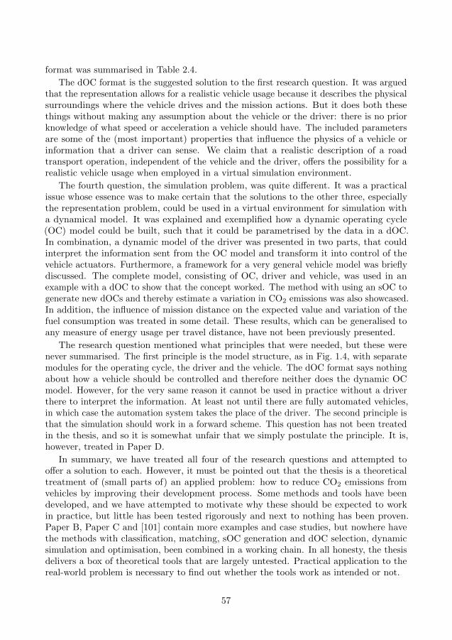
format was summarised in Table 2.4.

The dOC format is the suggested solution to the first research question. It was arguedthat the representation allows for a realistic vehicle usage because it describes the physicalsurroundings where the vehicle drives and the mission actions. But it does both thesethings without making any assumption about the vehicle or the driver: there is no priorknowledge of what speed or acceleration a vehicle should have. The included parametersare some of the (most important) properties that influence the physics of a vehicle orinformation that a driver can sense. We claim that a realistic description of a roadtransport operation, independent of the vehicle and the driver, offers the possibility for arealistic vehicle usage when employed in a virtual simulation environment.

The fourth question, the simulation problem, was quite different. It was a practicalissue whose essence was to make certain that the solutions to the other three, especiallythe representation problem, could be used in a virtual environment for simulation witha dynamical model. It was explained and exemplified how a dynamic operating cycle(OC) model could be built, such that it could be parametrised by the data in a dOC.In combination, a dynamic model of the driver was presented in two parts, that couldinterpret the information sent from the OC model and transform it into control of thevehicle actuators. Furthermore, a framework for a very general vehicle model was brieflydiscussed. The complete model, consisting of OC, driver and vehicle, was used in anexample with a dOC to show that the concept worked. The method with using an sOC togenerate new dOCs and thereby estimate a variation in CO2 emissions was also showcased.In addition, the influence of mission distance on the expected value and variation of thefuel consumption was treated in some detail. These results, which can be generalised toany measure of energy usage per travel distance, have not been previously presented.

The research question mentioned what principles that were needed, but these werenever summarised. The first principle is the model structure, as in Fig. 1.4, with separatemodules for the operating cycle, the driver and the vehicle. The dOC format says nothingabout how a vehicle should be controlled and therefore neither does the dynamic OCmodel. However, for the very same reason it cannot be used in practice without a driverthere to interpret the information. At least not until there are fully automated vehicles,in which case the automation system takes the place of the driver. The second principle isthat the simulation should work in a forward scheme. This question has not been treatedin the thesis, and so it is somewhat unfair that we simply postulate the principle. It is,however, treated in Paper D.

In summary, we have treated all four of the research questions and attempted tooffer a solution to each. However, it must be pointed out that the thesis is a theoreticaltreatment of (small parts of) an applied problem: how to reduce CO2 emissions fromvehicles by improving their development process. Some methods and tools have beendeveloped, and we have attempted to motivate why these should be expected to workin practice, but little has been tested rigorously and next to nothing has been proven.Paper B, Paper C and [101] contain more examples and case studies, but nowhere havethe methods with classification, matching, sOC generation and dOC selection, dynamicsimulation and optimisation, been combined in a working chain. In all honesty, the thesisdelivers a box of theoretical tools that are largely untested. Practical application to thereal-world problem is necessary to find out whether the tools work as intended or not.

57

4.2 Outlook

After having looked back at what was done, it is time to look in the opposite directionand outline some ways to continue.

There are suggested solutions for all research questions, but the one in the classificationproblem can be particularly improved. Three new questions appeared when solving theproblem, concerning how to choose classification metrics and labels in a systematic andscientific way. We later returned to these to comment that the parameters of the sOCformat would be suitable choices of metrics, which may be an answer to one or two of thenew questions. However, the remaining one (‘how can the classification limits be chosensystematically?’) has not been solved. It offers an interesting problem whose solution isnot obvious. In some sense, it is a matter of finding patterns and, therefore, employingmachine learning algorithms may be a direction to explore. Another way to continue withthe classification problem is to explicitly construct a bird’s eye view classification systemthat is open and available to everybody. This could be valuable both for the scientificcommunity and original equipment manufacturers.

The third research question and the sOC format have obvious extensions: stochasticmodels were only presented for properties in the road category. None were presentedfor the weather, the traffic or the mission. A stochastic approach is common for thetwo former, but not for the latter. How to construct such models is an interesting andunexplored question. It could also be quite challenging, because the mission category canhave a dependence both on time and space. Modelling this may require an innovativeapproach.

The first research question and the dOC format have similar extensions. The weatherand traffic categories have not been used to any larger extent, and very likely need morework before they are useful in practice. This is also true for some of the parameters in theroad category, especially the roughness and ground type. At the very least, examples ofdriver interaction (the tactical part of the driver model) and vehicle modules that can usethese concepts should be presented. That being said, the truly innovative part of the dOCformat, compared to other comprehensive road descriptions (like OpenDRIVE [149], theunofficial standard used in vehicle simulators), is the mission category. Considering thevast variety of different vehicle applications, there are bound to be many opportunities todevelop this further.

As far as the simulation problem is concerned, implementation can always be improvedbut that does not mean it is a research opportunity. However, the question was includedto serve as an insurance that the solutions to the other problems were useful in practice.With that mindset, the question can be expanded to a larger setting that concerns theentire development process: ‘what should a product development process look like to beeffective and are there basic principles it should follow?’. This was discussed in [101], butthe topic has been avoided in the thesis because too many tools were missing to continueworking with it at the time. With the development of the sOC format and the connectionsbetween the three levels of representation, those tools are now available and the research(presented in Fig. 4.1) can be continued. Especially, the development idea must be testedin practice; both numerically with dynamic simulations and experimentally with realusers and vehicles. This is what was referred to with the final remarks in Section 4.1.

58

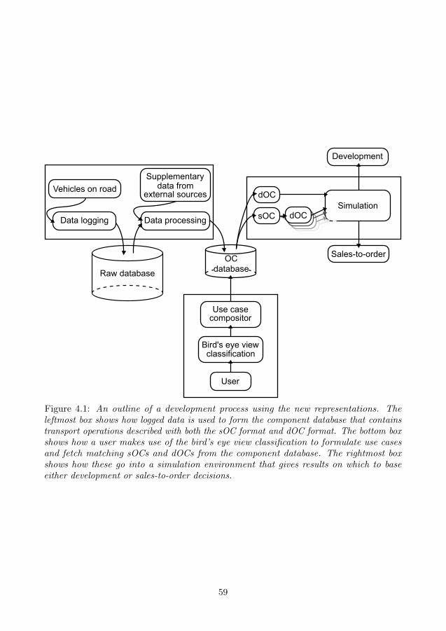
Vehicles on road

Data logging

Raw database

Data processing

dOC

sOC

User

Simulation

external sourcesdata from

Supplementary

Use casecompositor

Bird's eye viewclassification

dOC

OC

database

Development

Sales-to-order

Figure 4.1: An outline of a development process using the new representations. Theleftmost box shows how logged data is used to form the component database that containstransport operations described with both the sOC format and dOC format. The bottom boxshows how a user makes use of the bird’s eye view classification to formulate use casesand fetch matching sOCs and dOCs from the component database. The rightmost boxshows how these go into a simulation environment that gives results on which to baseeither development or sales-to-order decisions.

59

Another thing that we have not brought up in detail is logged data from vehiclesin normal operation. We have used it for some analysis, like Figs. 2.2, 2.3, 2.7 andTable 2.1, and the dOC in Fig. 2.8. Such data is a central part when working with therepresentations in practice. It tells us where a vehicle drives and what it does, givingthe details to the operations of many transport applications. Logged data is the pool ofinformation from which sOCs and dOCs can be estimated, as indicated by the left boxof Fig. 4.1. Although such data contains much information, it is contaminated by thedriver and the vehicle it originates from. This is a problem, because both the sOC formatand the dOC format are fundamentally driver and vehicle independent. One possiblesolution to filter unwanted influences is to use supplementary data from external sources,that do not contain such contaminations. External data would also make it possible tofind information that is not stored (like weather and traffic). There could be interestingquestions regarding the coupling between logged data and that from external sources:how to approach uncertainties and what data to trust; how to fuse information in a goodway; what to actually measure; and more.

The driver is the final thing that we will discuss. This was mentioned as one of thelimitations, and it was stated that the problem of how to model this person was not apart of the research questions. Then the representations and the dynamic OC model wereconstructed as driver independent. But there must still be a driver model in practicalsimulation, because something needs to interpret the road and convert this informationinto control of the appropriate vehicle interfaces. Subsequently, a driver in two partswas presented: a tactical module and a control module. This idea could be thoroughlyinvestigated, especially with experimental measurements in a driving simulator. Forinstance, one could design dedicated studies to find values for the parameters in thetactical module or investigate whether the simple relations between road properties andthe speed a driver wants hold.

60

References

[1] P. Pettersson, S. Berglund, H. Ryberg, B. Jacobson, G. Karlsson, L. Brusved, andJ. Bjernetun. Comparison of dual and single clutch transmission based on GlobalTransport Application mission profiles. International Journal of Vehicle Design77.1/2 (Mar. 2019), pp. 22–42. doi: 10.1504/IJVD.2018.098263.

[2] P. Pettersson, S. Berglund, B. Jacobson, L. Fast, P. Johannesson, and F. Santandrea.A proposal for an operating cycle description format for road transport missions.European Transport Research Review 10.31 (June 2018), pp. 1–19. doi: 10.1186/s12544-018-0298-4.

[3] P. Pettersson, P. Johannesson, B. Jacobson, F. Bruzelius, L. Fast, and S. Berglund.A statistical operating cycle description for prediction of road vehicles’ energyconsumption. Transportation Research Part D: Transport and Environment 73(Aug. 2019), pp. 205–229. doi: 10.1016/j.trd.2019.07.006.

[4] P. Pettersson, B. Jacobson, F. Bruzelius, P. Johannesson, and L. Fast. Intrinsicdifferences between backward and forward vehicle simulation models. Submitted to21st IFAC world congress. Oct. 2019.

[5] P. Pettersson, B. Jacobson, P. Johannesson, S. Berglund, and L. Laine. “Influenceof hill length on energy consumption for hybridized heavy transports in long haultransports”. 7th Commercial Vehicle Workshop Graz. Graz, Austria: TU Graz,May 2016. url: https://research.chalmers.se/publication/236668 (visitedon June 18, 2018).

[6] A. Odrigo, M. El-Gindy, P. Pettersson, Z. Nedelkova, P. Lindroth, and F. Oijer.Design and development of a road profile generator. International Journal ofVehicle Systems Modelling and Testing 11.3 (Dec. 2016), pp. 217–233. doi: 10.1504/IJVSMT.2016.080875.

[7] Copernicus Climate Change Service. Record-breaking temperatures for June. Tech.rep. Shinfield Park, Reading, U.K.: European Centre for Medium-Range WeatherForecasts, July 2, 2019. url: https : / / climate . copernicus . eu / record -

breaking-temperatures-june (visited on Aug. 15, 2019).[8] S. Scutti. Worldwide, June 2019 was the hottest June ever, according to more than

a century of weather records. CNN (July 19, 2019). url: https://edition.cnn.com/2019/07/19/us/june-2019-hottest-on-record/index.html (visited onAug. 15, 2019).

[9] C. Harvey. July Was the Hottest Month in Recorded History. Scientific American(Aug. 6, 2019). url: https://www.scientificamerican.com/article/july-was-the-hottest-month-in-recorded-history/ (visited on Oct. 17, 2019).

[10] Union of concerned scientists. Global warming. Tech. rep. Cambridge, MA, U.S:Union of concerned scientists, 2019. url: https://www.ucsusa.org/our-work/global-warming/science-and-impacts/global-warming-science (visited onAug. 15, 2019).

[11] J. Cook, D. Nuccitelli, S. A. Green, M. Richardson, B. Winkler, R. Painting,R. Way, P. Jacobs, and A. Skuce. Quantifying the consensus on anthropogenicglobal warming in the scientific literature. Environ. Res. Lett. 8.2 (May 2013). doi:

61


https://doi.org/10.1186/s12544-018-0298-4

https://doi.org/10.1186/s12544-018-0298-4





https://climate.copernicus.eu/record-breaking-temperatures-june

https://climate.copernicus.eu/record-breaking-temperatures-june

https://edition.cnn.com/2019/07/19/us/june-2019-hottest-on-record/index.html

https://edition.cnn.com/2019/07/19/us/june-2019-hottest-on-record/index.html

https://www.scientificamerican.com/article/july-was-the-hottest-month-in-recorded-history/

https://www.scientificamerican.com/article/july-was-the-hottest-month-in-recorded-history/

https://www.ucsusa.org/our-work/global-warming/science-and-impacts/global-warming-science

https://www.ucsusa.org/our-work/global-warming/science-and-impacts/global-warming-science

10.1088/1748-9326/8/2/024024. url: https://doi.org/10.1088%2F1748-9326%2F8%2F2%2F024024 (visited on Aug. 15, 2019).

[12] S. Callery. Climate Change: How Do We Know. Tech. rep. Two independencesquare, Washington D.C., U.S.: NASA, 2019. url: https://climate.nasa.gov/evidence/ (visited on Aug. 15, 2019).

[13] Princeton University. A more potent greenhouse gas than carbon dioxide, methaneemissions will leap as Earth warms. ScienceDaily (Mar. 27, 2014). url: www.

sciencedaily.com/releases/2014/03/140327111724.htm (visited on Aug. 15,2019).

[14] United States Environmental Protection Agency. Overview of Greenhouse Gases.Tech. rep. Washington D.C., U.S.: United States Environmental Protection Agency,Apr. 11, 2019. url: https://www.epa.gov/ghgemissions/overview-greenhouse-gases (visited on Aug. 15, 2019).

[15] C. Le Quere, R. M. Andrew, and P. e. a. Friedlingstein. Global Carbon Budget 2018.Earth System Science Data 10.4 (Dec. 5, 2018), pp. 2141–2194. doi: 10.5194/essd-10-2141-2018. url: https://www.earth-syst-sci-data.net/10/2141/2018/(visited on Aug. 15, 2019).

[16] Eurostat. Greenhouse gas emission statistics - emission inventories. Tech. rep.Rue Alphonse Weicker, Luxembourg: EU commission, June 2019. url: https://ec.europa.eu/eurostat/statistics- explained/pdfscache/1180.pdf

(visited on Aug. 15, 2019).[17] E. E. Agency. Greenhouse gas emissions from transport. Tech. rep. European En-

vironment Agency, July 12, 2019. url: https://www.eea.europa.eu/data-and-maps/indicators/transport-emissions-of-greenhouse-gases/transport-

emissions-of-greenhouse-gases-11 (visited on Aug. 16, 2019).[18] Global Carbon Project. The global carbon atlas, CO2 emissions. 2017. url: http:

//www.globalcarbonatlas.org/en/CO2-emissions (visited on Sept. 30, 2019).[19] United Nations Framework Convention on Climate Change. Kyoto Protocol to

the United Nations Framework Convention on Climate Change. No. 30822. Kyoto,Japan, Feb. 2005. url: https://treaties.un.org/pages/ViewDetails.aspx?src=TREATY&mtdsg_no=XXVII-7-a&chapter=27&lang=en (visited on Apr. 27,2017).

[20] United Nations Framework Convention on Climate Change. Paris Agreement.No. 54113. Paris, France, Nov. 2016. url: https://treaties.un.org/pages/ViewDetails.aspx?src=TREATY&mtdsg_no=XXVII-7-d&chapter=27&clang=_en

(visited on Apr. 27, 2017).[21] European Commission. Regulation (EU) No 333/2014 of the European Parliament

and of the Council of 11 March 2014 amending Regulation (EC) No 443/2009 todefine the modalities for reaching the 2020 target to reduce CO2 emissions fromnew passenger cars. Official Journal of the European Union 57.L 103 (Apr. 2014).url: https://eur-lex.europa.eu/legal-content/EN/TXT/?uri=OJ:L:2014:084:TOC (visited on Sept. 27, 2019).

[22] European Commission. Regulation (EU) No 253/2014 of the European Parliamentand of the Council of 26 February 2014 amending Regulation (EU) No 510/2011 todefine the modalities for reaching the 2020 target to reduce CO2 emissions from new

62

https://doi.org/10.1088/1748-9326/8/2/024024

https://doi.org/10.1088%2F1748-9326%2F8%2F2%2F024024

https://doi.org/10.1088%2F1748-9326%2F8%2F2%2F024024

https://climate.nasa.gov/evidence/

https://climate.nasa.gov/evidence/

www.sciencedaily.com/releases/2014/03/140327111724.htm

www.sciencedaily.com/releases/2014/03/140327111724.htm

https://www.epa.gov/ghgemissions/overview-greenhouse-gases

https://www.epa.gov/ghgemissions/overview-greenhouse-gases

https://doi.org/10.5194/essd-10-2141-2018

https://doi.org/10.5194/essd-10-2141-2018

https://www.earth-syst-sci-data.net/10/2141/2018/

https://ec.europa.eu/eurostat/statistics-explained/pdfscache/1180.pdf

https://ec.europa.eu/eurostat/statistics-explained/pdfscache/1180.pdf

https://www.eea.europa.eu/data-and-maps/indicators/transport-emissions-of-greenhouse-gases/transport-emissions-of-greenhouse-gases-11



http://www.globalcarbonatlas.org/en/CO2-emissions

http://www.globalcarbonatlas.org/en/CO2-emissions

https://treaties.un.org/pages/ViewDetails.aspx?src=TREATY&mtdsg_no=XXVII-7-a&chapter=27&lang=en

https://treaties.un.org/pages/ViewDetails.aspx?src=TREATY&mtdsg_no=XXVII-7-a&chapter=27&lang=en

https://treaties.un.org/pages/ViewDetails.aspx?src=TREATY&mtdsg_no=XXVII-7-d&chapter=27&clang=_en

https://treaties.un.org/pages/ViewDetails.aspx?src=TREATY&mtdsg_no=XXVII-7-d&chapter=27&clang=_en

https://eur-lex.europa.eu/legal-content/EN/TXT/?uri=OJ:L:2014:084:TOC


light commercial vehicles (1). Official Journal of the European Union 57.L 084 (Mar.2014). url: https://eur-lex.europa.eu/legal-content/EN/TXT/?uri=OJ:L:2014:084:TOC (visited on Sept. 27, 2019).

[23] European Commission. Regulation (EU) 2019/1242 of the European Parliamentand of the Council of 20 June 2019 setting CO2 emission performance standards fornew heavy-duty vehicles and amending Regulations (EC) No 595/2009 and (EU)2018/956 of the European Parliament and of the Council and Council Directive96/53/EC ( 1 ). Brussel, Belgium, July 25, 2019. url: https://eur-lex.europa.eu/legal-content/EN/TXT/HTML/?uri=OJ:L:2019:198:FULL&from=EN (visitedon Aug. 23, 2019).

[24] M. Tutuianu, P. Bonnel, B. Ciuffo, T. Haniu, N. Ichikawa, A. Marotta, J. Pavlovic,and H. Steven. Development of the World-wide harmonized light duty test cycle(WLTC) and a possible pathway for its introduction in the European legislation.Transportation research part D: transport and environment 40.1 (2015), pp. 61–75.doi: 10.1016/j.trd.2015.07.011.

[25] S. Edlund and P. O. Fryk. “The Right Truck for the Job with Global TruckApplication Descriptions”. SAE technical paper 2004-01-2645. Oct. 2004. doi:10.4271/2004-01-2645.

[26] G. Fontaras, M. Rexeis, S. Hausberger, A. Kies, J. Hammer, L. E. Schulte, K.Anagnostopoulos, U. Manfredi, M. Carriero, and P. Dilara. Development of aCO2 certification and monitoring methodology for a heavy duty vehicles - proof ofconcept report. Technical report EUR 26452. Ispra, Italy: Joint Research centre,2014.

[27] P. Lindroth. “Product Configuration from a Mathematical Optimization Perspec-tive”. PhD thesis. Goteborg, Sweden: Chalmers University of Technology, 2011.url: https://research.chalmers.se/publication/140022 (visited on Apr. 4,2018).

[28] European Commission. Commission Regulation (EU) 2017/2400. Official Journalof the European Union 60.L 349 (Dec. 2017). url: https://eur-lex.europa.eu/legal-content/EN/TXT/?uri=OJ:L:2017:349:TOC (visited on Aug. 27, 2019).

[29] G. Fontaras, M. Rexeis, P. Dilara, S. Hausberger, and K. Anagnostopoulos. “TheDevelopment of a Simulation Tool for Monitoring Heavy-Duty Vehicle CO2 Emis-sions and Fuel Consumption in Europe”. 11th International Conference on Engines& Vehicles. Sept. 8, 2013. doi: 10.4271/2013-24-0150.

[30] Joint Research Centre. “VECTO - overview”. 2018 VECTO workshop. Ispra,Italy, Nov. 2018. url: https://ec.europa.eu/clima/sites/clima/files/transport/vehicles/vecto/201811_overview_en.pdf (visited on Oct. 30,2019).

[31] European commission. Vecto user manual. 3.3.1. European Union. Rue de la Loi,Brussel, Feb. 1, 2019. url: https://ec.europa.eu/clima/policies/transport/vehicles/vecto_en (visited on July 26, 2019).

[32] J. Weber. “Automotive development processes”. Dordrecht; New York: Springer,2009. Chap. 4, pp. 41–52.

[33] B. Jacobson. “Gear Shifting with Retained Power Transfer”. PhD thesis. Goteborg,Sweden: Chalmers University of Technology, 1993.

63



https://eur-lex.europa.eu/legal-content/EN/TXT/HTML/?uri=OJ:L:2019:198:FULL&from=EN

https://eur-lex.europa.eu/legal-content/EN/TXT/HTML/?uri=OJ:L:2019:198:FULL&from=EN


https://doi.org/10.4271/2004-01-2645




https://doi.org/10.4271/2013-24-0150

https://ec.europa.eu/clima/sites/clima/files/transport/vehicles/vecto/201811_overview_en.pdf

https://ec.europa.eu/clima/sites/clima/files/transport/vehicles/vecto/201811_overview_en.pdf

https://ec.europa.eu/clima/policies/transport/vehicles/vecto_en


[34] J. Happian-Smith. Introduction to Modern Vehicle Design. 1st ed. Oxford, U.K.:Butterworth Heinemann, 2001, pp. 553–571.

[35] J. Wong. Theory of ground vehicles. 4th ed. Hoboken, NJ, U.S.: John Wiley &Sons, 2008.

[36] H. Pacejka. Tire and Vehicle Dynamics. 3rd ed. Oxford, UK: Elsevier/Butterworth-Heinemann, 2012.

[37] J. B. Heywood. Internal combustion engine fundamentals. Internat. ed. New York,U.S.: McGraw-Hill, 1988.

[38] L. Eriksson and L. Nielsen. Modeling and control of engines and drivelines. 1st ed.Chichester, West Sussex, United Kingdom: Wiley, 2014.

[39] L. Guzzella and A. Sciarretta. Vehicle propulsion systems: introduction to modelingand optimization. 3rd ed. Berlin, Germany: Springer, 2013.

[40] A. Stokes. Manual gearbox design. 1st ed. Oxford, UK: Butterworth-Heinemann,1992.

[41] G. Mastinu and M. Ploechl. Road and off-road vehicle system dynamics handbook.1st ed. FL, U.S.: CRC Press, 2014.

[42] D. W. Wyatt, H. Li, and J. E. Tate. The impact of road grade on carbon dioxide(CO2) emission of a passenger vehicle in real-world driving. Transportation ResearchPart D: Transport and Environment 32 (2014), pp. 160–170. doi: 10.1016/j.trd.2014.07.015.

[43] K. M. Sentoff, L. Aultman-Hall, and B. A. Holmen. Implications of driving styleand road grade for accurate vehicle activity data and emissions estimates. Trans-portation Research Part D: Transport and Environment 35 (2015), pp. 175–188.doi: 10.1016/j.trd.2014.11.021.

[44] K. Liu, T. Yamamoto, and T. Morikawa. Impact of road gradient on energyconsumption of electric vehicles. Transportation Research Part D: Transport andEnvironment 54 (2017), pp. 74–81. doi: https://doi.org/10.1016/j.trd.2017.05.005.

[45] O. Travesset-Baro, M. Rosas-Casals, and E. Jover. Transport energy consumptionin mountainous roads. A comparative case study for internal combustion enginesand electric vehicles in Andorra. Transportation Research Part D: Transport andEnvironment 34 (Jan. 2015), pp. 16–26. doi: 10.1016/j.trd.2014.09.006.url: https://linkinghub.elsevier.com/retrieve/pii/S1361920914001424(visited on Aug. 21, 2019).

[46] B. Yazdani Boroujeni and H. C. Frey. Road grade quantification based on globalpositioning system data obtained from real-world vehicle fuel use and emissionsmeasurements. Atmospheric Environment 85 (Mar. 2014), pp. 179–186. doi: 10.1016/j.atmosenv.2013.12.025. url: https://linkinghub.elsevier.com/retrieve/pii/S1352231013009709 (visited on Aug. 21, 2019).

[47] P. Sahlholm. “Distributed road grade estimation for heavy duty vehicles”. OCLC:732293828. PhD thesis. Stockholm,Sweden: Electrical Engineering, KTH RoyalInstitute of Technology, 2011. url: http://urn.kb.se/resolve?urn=urn:nbn:se:kth:diva-32054%20urn:nbn:se:kth:diva-32054 (visited on Aug. 21, 2019).

64




https://doi.org/https://doi.org/10.1016/j.trd.2017.05.005



https://linkinghub.elsevier.com/retrieve/pii/S1361920914001424

https://doi.org/10.1016/j.atmosenv.2013.12.025




http://urn.kb.se/resolve?urn=urn:nbn:se:kth:diva-32054%20urn:nbn:se:kth:diva-32054

http://urn.kb.se/resolve?urn=urn:nbn:se:kth:diva-32054%20urn:nbn:se:kth:diva-32054

[48] E. Wood, A. Duran, E. Burton, J. Gonder, and K. Kelly. EPA GHG Certifica-tion of Medium- and Heavy-Duty Vehicles: Development of Road Grade ProfilesRepresentative of US Controlled Access Highways. Renewable Energy (2015), p. 79.

[49] J. Han, D. Kum, and Y. Park. Impact of hilly road information on fuel economyof FCHEV based on parameterization of hilly roads. Int.J Automot. Technol.15.2 (Mar. 1, 2014), pp. 283–290. doi: 10.1007/s12239- 014- 0029- 3. url:https://doi.org/10.1007/s12239-014-0029-3 (visited on Aug. 23, 2019).

[50] D. Llopis-Castello, A. M. Perez-Zuriaga, F. J. Camacho-Torregrosa, and A. Garcıa.Impact of horizontal geometric design of two-lane rural roads on vehicle co2emissions. Transportation Research Part D: Transport and Environment 59 (2018),pp. 46–57. doi: 10.1016/j.trd.2017.12.020.

[51] A. Louhghalam, M. Akbarian, and F. J. Ulm. Roughness-Induced Pavement-Vehicle Interactions: Key Parameters and Impact on Vehicle Fuel Consumption.Transportation Research Record 2525.1 (Jan. 1, 2015), pp. 62–70. doi: 10.3141/2525-07. (Visited on Aug. 22, 2019).

[52] W. Li, P. Stanula, P. Egede, S. Kara, and C. Herrmann. Determining the MainFactors Influencing the Energy Consumption of Electric Vehicles in the Usage Phase.Procedia CIRP 48 (2016), pp. 352–357. doi: 10.1016/j.procir.2016.03.014.url: https://linkinghub.elsevier.com/retrieve/pii/S221282711600651X(visited on Aug. 21, 2019).

[53] C. Liu, Y. O. Susilo, and A. Karlstrom. Estimating changes in transport CO2emissions due to changes in weather and climate in Sweden. Transportation ResearchPart D: Transport and Environment 49 (Dec. 1, 2016), pp. 172–187. doi: 10.1016/j.trd.2016.09.004. url: http://www.sciencedirect.com/science/article/pii/S1361920915301085 (visited on Aug. 21, 2019).

[54] G. M. Fetene, S. Kaplan, S. L. Mabit, A. F. Jensen, and C. G. Prato. Harnessingbig data for estimating the energy consumption and driving range of electricvehicles. Transportation Research Part D: Transport and Environment 54 (July2017), pp. 1–11. doi: 10.1016/j.trd.2017.04.013. url: https://linkinghub.elsevier.com/retrieve/pii/S1361920917303188 (visited on Aug. 21, 2019).

[55] A. Braun and W. Rid. Assessing driving pattern factors for the specific energy use ofelectric vehicles: a factor analysis approach from case study data of the Mitsubishii-MiEV minicar. Transportation Research Part D: Transport and Environment 58(Jan. 2018), pp. 225–238. doi: 10.1016/j.trd.2017.11.011.

[56] H. Achour and A. Olabi. Driving cycle developments and their impacts on en-ergy consumption of transportation. Journal of Cleaner Production 112 (Jan.2016), pp. 1778–1788. doi: 10.1016/j.jclepro.2015.08.007. url: https:

//linkinghub.elsevier.com/retrieve/pii/S0959652615010963 (visited onAug. 23, 2019).

[57] J. Liu, X. Wang, and A. Khattak. Customizing driving cycles to support vehiclepurchase and use decisions: Fuel economy estimation for alternative fuel vehicleusers. Transportation Research Part C: Emerging Technologies 67 (2016), pp. 280–298. doi: https://doi.org/10.1016/j.trc.2016.02.016.

[58] P. Shen, Z. Zhao, J. Li, and X. Zhan. Development of a typical driving cycle foran intra-city hybrid electric bus with a fixed route. Transportation Research Part

65

https://doi.org/10.1007/s12239-014-0029-3

https://doi.org/10.1007/s12239-014-0029-3


https://doi.org/10.3141/2525-07

https://doi.org/10.3141/2525-07

https://doi.org/10.1016/j.procir.2016.03.014

https://linkinghub.elsevier.com/retrieve/pii/S221282711600651X



http://www.sciencedirect.com/science/article/pii/S1361920915301085






https://doi.org/10.1016/j.jclepro.2015.08.007



https://doi.org/https://doi.org/10.1016/j.trc.2016.02.016

D: Transport and Environment 59 (2018), pp. 346–360. doi: https://doi.org/10.1016/j.trd.2018.01.032. url: http://www.sciencedirect.com/science/article/pii/S1361920917303218.

[59] J. Brady and M. O’Mahony. Development of a driving cycle to evaluate theenergy economy of electric vehicles in urban areas. Applied Energy 177 (2016),pp. 165–178. doi: https://doi.org/10.1016/j.apenergy.2016.05.094. url:http://www.sciencedirect.com/science/article/pii/S0306261916306924.

[60] P. Nyberg. “Evaluation, generation and transformation of driving cycles”. PhDthesis. Linkoping, Sweden: Vehicular systems, Linkoping University, 2015.

[61] J. Vepsalainen, K. Kivekas, K. Otto, A. Lajunen, and K. Tammi. Development andvalidation of energy demand uncertainty model for electric city buses. Transporta-tion Research Part D: Transport and Environment 63 (Aug. 1, 2018), pp. 347–361.doi: 10.1016/j.trd.2018.06.004.

[62] A. Ashtari, E. Bibeau, and S. Shahidinejad. Using large driving record samples anda stochastic approach for real-world driving cycle construction: Winnipeg drivingcycle. Transportation Science 48.2 (May 2014), pp. 170–183. doi: 10.1287/trsc.1120.0447.

[63] T. K. Lee and Z. S. Filipi. Synthesis of real-world driving cycles using stochasticprocess and statistical methodology. International Journal of Vehicle Design 57.1(2011), pp. 17–36. doi: 10.1504/IJVD.2011.043590.

[64] M. Asbogard, L. Johannesson, D. Angervall, and P. Johansson. “Improving SystemDesign of a Hybrid Powertrain Using Stochastic Drive Cycles and Dynamic Pro-gramming”. SAE World Congress and Exhibition. Detroit, MI, USA, Apr. 16, 2007.doi: 10.4271/2007-01-0304. url: http://papers.sae.org/2007-01-0304/(visited on Aug. 5, 2018).

[65] M. Pourabdollah, A. Grauers, and B. Egardt. Effect of Driving patterns on Com-ponents sizing of a Series PHEV. IFAC Proceedings Volumes 46.21 (Jan. 1, 2013),pp. 17–22. doi: 10.3182/20130904- 4- JP- 2042.00013. url: http://www.

sciencedirect.com/science/article/pii/S1474667016383367 (visited onAug. 27, 2019).

[66] P. Nyberg, E. Frisk, and L. Nielsen. Driving Cycle Equivalence and Transformation.IEEE Transactions on Vehicular Technology 66.3 (Mar. 2017), pp. 1963–1974. doi:10.1109/TVT.2016.2582079.

[67] K. Hereijgers, E. Silvas, T. Hofman, and M. Steinbuch. Effects of using SynthesizedDriving Cycles on Vehicle Fuel Consumption. IFAC-PapersOnLine 50.1 (July2017), pp. 7505–7510. doi: 10.1016/j.ifacol.2017.08.1183. url: https:

//linkinghub.elsevier.com/retrieve/pii/S2405896317316816 (visited onAug. 28, 2019).

[68] M. Fries, A. Baum, M. Wittmann, and M. Lienkamp. “Derivation of a real-lifedriving cycle from fleet testing data with the Markov-Chain-Monte-Carlo Method”.2018 21st International Conference on Intelligent Transportation Systems (ITSC).Maui, HI: IEEE, Nov. 2018, pp. 2550–2555. doi: 10.1109/ITSC.2018.8569547.url: https://ieeexplore.ieee.org/document/8569547/ (visited on Aug. 28,2019).

66





https://doi.org/https://doi.org/10.1016/j.apenergy.2016.05.094



https://doi.org/10.1287/trsc.1120.0447

https://doi.org/10.1287/trsc.1120.0447


https://doi.org/10.4271/2007-01-0304

http://papers.sae.org/2007-01-0304/

https://doi.org/10.3182/20130904-4-JP-2042.00013



https://doi.org/10.1109/TVT.2016.2582079

https://doi.org/10.1016/j.ifacol.2017.08.1183



https://doi.org/10.1109/ITSC.2018.8569547

https://ieeexplore.ieee.org/document/8569547/

[69] G. Souffran, L. Miegeville, and P. Guerin. Simulation of Real-World VehicleMissions Using a Stochastic Markov Model for Optimal Powertrain Sizing. IEEETransactions on Vehicular Technology 61.8 (Oct. 2012), pp. 3454–3465. doi: 10.1109/TVT.2012.2206618. url: http://ieeexplore.ieee.org/document/

6227377/ (visited on Aug. 28, 2019).[70] J. D. Bishop, C. J. Axon, and M. D. McCulloch. A robust, data-driven method-

ology for real-world driving cycle development. Transportation Research PartD: Transport and Environment 17.5 (July 2012), pp. 389–397. doi: 10.1016/j.trd.2012.03.003. url: https://linkinghub.elsevier.com/retrieve/pii/S136192091200034X (visited on Aug. 28, 2019).

[71] G. Fontaras, T. Grigoratos, D. Savvidis, K. Anagnostopoulos, R. Luz, M. Rexeis,and S. Hausberger. An experimental evaluation of the methodology proposed for themonitoring and certification of CO2 emissions from heavy-duty vehicles in Europe.Energy 102 (May 2016), pp. 354–364. doi: 10.1016/j.energy.2016.02.076.url: https://linkinghub.elsevier.com/retrieve/pii/S0360544216301384(visited on Aug. 22, 2019).

[72] Joint Research Centre. Vecto user manual. 3.3.1. European Union. Rue de laLoi, Brussel, Feb. 1, 2019. url: https://ec.europa.eu/clima/policies/

transport/vehicles/vecto_en (visited on July 26, 2019).[73] A. Arikere and A. Tysk. Added Value for Electrified Vehicles through Enhanced

Active Safety. World Electric Vehicle Journal 8.3 (Sept. 2016), pp. 623–634. doi:10.3390/wevj8030623. url: https://www.mdpi.com/2032-6653/8/3/623(visited on Aug. 22, 2019).

[74] A. Arikere. “Vehicle dynamics control for active safety functions using electrifieddrivelines”. PhD thesis. Gothenburg, Sweden: Chalmers University of Technology,Apr. 2018.

[75] S. Berglund. “Modeling complex engines as dynamic powertrain members”. PhDthesis. Gothenburg, Sweden: Chalmers University of Technology, July 1999.

[76] B. Jacobson. “Vehicle dynamics”. 2018th ed. Gothenburg, Sweden: ChalmersUniversity of Technology, 2018. Chap. 3, pp. 137–174.

[77] L. Johnson and A. J. Nedzesky. A comparative study of speed humps, speed slitsand speed cushions. Tech. rep. Annual meeting compendium. Washington, DC,U.S.: U.S. Department of Transportation Federal Highway Administration, 2004.

[78] AB Volvo. Predictive cruise control I-SEE. Accessed: 2017-03-01. 2016. url: http://www.volvotrucks.us/powertrain/i-shift-transmission/i-see/ (visitedon Mar. 1, 2017).

[79] Scania AB. Spectacular fuel savings - Scania Opticruise with performance modes. Ac-cessed: 2017-03-01. 2013. url: https://www.scania.com/group/en/spectacular-fuel-savings-scania-opticruise-with-%20performance-modes/ (visited onMar. 1, 2017).

[80] Daimler AG. Predictive powertrain control - clever cruise control helps save fuel. Ac-cessed: 2017-03-01. 2012. url: http://media.daimler.com/marsMediaSite/en/instance/ko/Predictive-Powertrain-Control---Clever-cruise-%20control-

helps-.xhtml?oid=9917205 (visited on Mar. 1, 2017).

67

https://doi.org/10.1109/TVT.2012.2206618

https://doi.org/10.1109/TVT.2012.2206618

http://ieeexplore.ieee.org/document/6227377/

http://ieeexplore.ieee.org/document/6227377/





https://doi.org/10.1016/j.energy.2016.02.076




https://doi.org/10.3390/wevj8030623

https://www.mdpi.com/2032-6653/8/3/623

http://www.volvotrucks.us/powertrain/i-shift-transmission/i-see/

http://www.volvotrucks.us/powertrain/i-shift-transmission/i-see/

https://www.scania.com/group/en/spectacular-fuel-savings-scania-opticruise-with-%20performance-modes/

https://www.scania.com/group/en/spectacular-fuel-savings-scania-opticruise-with-%20performance-modes/

http://media.daimler.com/marsMediaSite/en/instance/ko/Predictive-Powertrain-Control---Clever-cruise-%20control-helps-.xhtml?oid=9917205



[81] S. Torabi and M. Wahde. “Fuel consumption optimization of heavy-duty vehiclesusing genetic algorithms”. 2017 IEEE Congress on Evolutionary Computation(CEC). Red Hook, NY, U.S.: IEEE, June 2017, pp. 29–36. doi: 10.1109/CEC.2017.7969292.

[82] S. H. Hamdar, L. Qin, and A. Talebpour. Weather and road geometry impact onlongitudinal driving behavior: Exploratory analysis using an empirically supportedacceleration modeling framework. Transportation Research Part C: EmergingTechnologies 67 (June 2016), pp. 193–213. doi: 10.1016/j.trc.2016.01.017.url: https://linkinghub.elsevier.com/retrieve/pii/S0968090X1600036X(visited on Aug. 22, 2019).

[83] A. E. af Wahlberg. Long-term effects of training in economical driving: Fuelconsumption, accidents, driver acceleration behavior and technical feedback. In-ternational Journal of Industrial Ergonomics 37.4 (Apr. 2007), pp. 333–343. doi:10.1016/j.ergon.2006.12.003. url: https://linkinghub.elsevier.com/retrieve/pii/S016981410600268X (visited on Sept. 30, 2019).

[84] J. de Abreu e Silva, F. Moura, B. Garcia, and R. Vargas. Influential vectorsin fuel consumption by an urban bus operator: Bus route, driver behavior orvehicle type? Transportation Research Part D: Transport and Environment 38(July 2015), pp. 94–104. doi: 10 . 1016 / j . trd . 2015 . 04 . 003. url: https :

//linkinghub.elsevier.com/retrieve/pii/S1361920915000358 (visited onSept. 30, 2019).

[85] W.-T. Lai. The effects of eco-driving motivation, knowledge and reward interventionon fuel efficiency. Transportation Research Part D: Transport and Environment34 (Jan. 2015), pp. 155–160. doi: 10.1016/j.trd.2014.10.003. url: https://linkinghub.elsevier.com/retrieve/pii/S1361920914001448 (visited onAug. 22, 2019).

[86] I. Jeffreys, G. Graves, and M. Roth. Evaluation of eco-driving training for vehiclefuel use and emission reduction: A case study in Australia. Transportation ResearchPart D: Transport and Environment 60 (May 2018). doi: 10 . 1016 / j . trd .

2015 . 12 . 017. url: https : / / linkinghub . elsevier . com / retrieve / pii /

S1361920915002278 (visited on Aug. 22, 2019).[87] S. H. Ho, Y. D. Wong, and V. W. C. Chang. Developing Singapore Driving

Cycle for passenger cars to estimate fuel consumption and vehicular emissions.Atmospheric Environment 97 (Nov. 1, 2014), pp. 353–362. doi: 10.1016/j.

atmosenv.2014.08.042. url: http://www.sciencedirect.com/science/

article/pii/S135223101400644X (visited on Dec. 13, 2018).[88] G. Amirjamshidi and M. J. Roorda. Development of simulated driving cycles for

light, medium, and heavy duty trucks: Case of the Toronto Waterfront Area. Trans-portation Research Part D: Transport and Environment 34 (Jan. 1, 2015), pp. 255–266. doi: 10.1016/j.trd.2014.11.010. url: http://www.sciencedirect.com/science/article/pii/S1361920914001734 (visited on Dec. 13, 2018).

[89] N. H. Arun, S. Mahesh, G. Ramadurai, and S. M. S. Nagendra. Development ofdriving cycles for passenger cars and motorcycles in Chennai, India. SustainableCities and Society 32 (2017), pp. 508–512. doi: https://doi.org/10.1016/j.

68

https://doi.org/10.1109/CEC.2017.7969292

https://doi.org/10.1109/CEC.2017.7969292

https://doi.org/10.1016/j.trc.2016.01.017

https://linkinghub.elsevier.com/retrieve/pii/S0968090X1600036X

https://doi.org/10.1016/j.ergon.2006.12.003















http://www.sciencedirect.com/science/article/pii/S135223101400644X

http://www.sciencedirect.com/science/article/pii/S135223101400644X




https://doi.org/https://doi.org/10.1016/j.scs.2017.05.001



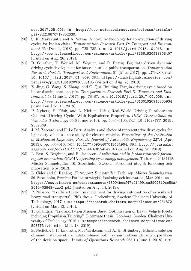
scs.2017.05.001. url: http://www.sciencedirect.com/science/article/pii/S2210670717302330.

[90] S. K. Mayakuntla and A. Verma. A novel methodology for construction of drivingcycles for Indian cities. Transportation Research Part D: Transport and Environ-ment 65 (Dec. 1, 2018), pp. 725–735. doi: 10.1016/j.trd.2018.10.013. url:http://www.sciencedirect.com/science/article/pii/S1361920918303407

(visited on Aug. 26, 2019).[91] R. Gunther, T. Wenzel, M. Wegner, and R. Rettig. Big data driven dynamic

driving cycle development for busses in urban public transportation. TransportationResearch Part D: Transport and Environment 51 (Mar. 2017), pp. 276–289. doi:10.1016/j.trd.2017.01.009. url: https://linkinghub.elsevier.com/

retrieve/pii/S1361920916308185 (visited on Aug. 26, 2019).[92] Z. Jing, G. Wang, S. Zhang, and C. Qiu. Building Tianjin driving cycle based on

linear discriminant analysis. Transportation Research Part D: Transport and Envi-ronment 53 (June 1, 2017), pp. 78–87. doi: 10.1016/j.trd.2017.04.005. url:http://www.sciencedirect.com/science/article/pii/S1361920916305934

(visited on Dec. 13, 2018).[93] P. Nyberg, E. Frisk, and L. Nielsen. Using Real-World Driving Databases to

Generate Driving Cycles With Equivalence Properties. IEEE Transactions onVehicular Technology 65.6 (June 2016), pp. 4095–4105. doi: 10.1109/TVT.2015.2502069.

[94] J. M. Zaccardi and F. Le Berr. Analysis and choice of representative drive cycles forlight duty vehicles - case study for electric vehicles. Proceedings of the Institutionof Mechanical Engineers, Part D: Journal of Automobile Engineering 227.4 (Apr.2013), pp. 605–616. doi: 10.1177/0954407012454964. url: http://journals.sagepub.com/doi/10.1177/0954407012454964 (visited on Aug. 26, 2019).

[95] L. Fast, S. Berglund, and B. Jacobson. Application within fordonsstrategisk forskn-ing och innovation: OCEAN operating cycle energy management. Tech. rep. 20131118.Master Samuelsgatan 16, Stockholm, Sweden: Fordonsstrategisk forskning ochinnovation, Nov. 2013.

[96] L. Cider and S. Ranang. Slutrapport Duo2-trailer. Tech. rep. Master Samuelsgatan56, Stockholm, Sweden: Fordonsstrategisk forskning och innovation, Mar. 2014. url:https://www.vinnova.se/contentassets/f3004bccf47a4f4991ca3909810ce50a/

2010-02849-duo2.pdf (visited on Aug. 14, 2019).[97] P. Nilsson. “Traffic situation management for driving automation of articulated

heavy road transports”. PhD thesis. Gothenburg, Sweden: Chalmers University ofTechnology, 2017. url: https://research.chalmers.se/publication/251872(visited on Mar. 13, 2019).

[98] T. Ghandriz. “Transportation Mission Based Optimization of Heavy Vehicle Fleetsincluding Propulsion Tailoring”. Licentiate thesis. Goteborg, Sweden: Chalmers Uni-versity of Technology, 2018. url: https://research.chalmers.se/publication/505773 (visited on Mar. 13, 2019).

[99] Z. Nedelkova, P. Lindroth, M. Patriksson, and A. B. Stromberg. Efficient solutionof many instances of a simulation-based optimization problem utilizing a partitionof the decision space. Annals of Operations Research 265.1 (June 1, 2018). doi:

69













https://doi.org/10.1109/TVT.2015.2502069

https://doi.org/10.1109/TVT.2015.2502069

https://doi.org/10.1177/0954407012454964

http://journals.sagepub.com/doi/10.1177/0954407012454964

http://journals.sagepub.com/doi/10.1177/0954407012454964

https://www.vinnova.se/contentassets/f3004bccf47a4f4991ca3909810ce50a/2010-02849-duo2.pdf

https://www.vinnova.se/contentassets/f3004bccf47a4f4991ca3909810ce50a/2010-02849-duo2.pdf




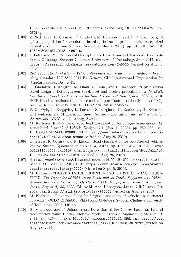
10.1007/s10479-017-2721-y. url: https://doi.org/10.1007/s10479-017-2721-y.

[100] Z. Nedelkova, C. Cromvik, P. Lindroth, M. Patriksson, and A. B. Stromberg. Asplitting algorithm for simulation-based optimization problems with categoricalvariables. Engineering Optimization 51.5 (May 4, 2019), pp. 815–831. doi: 10.1080/0305215X.2018.1495716.

[101] P. Pettersson. “On Numerical Descriptions of Road Transport Missions”. Licentiatethesis. Goteborg, Sweden: Chalmers University of Technology, June 2017. url:https://research.chalmers.se/publication/249525 (visited on Aug. 6,2018).

[102] ISO 8855. Road vehicles – Vehicle dynamics and road-holding ability – Vocab-ulary. Standard ISO 8855:2011(E). Geneva, CH: International Organization forStandardization, Dec. 2011.

[103] T. Ghandriz, J. Hellgren, M. Islam, L. Laine, and B. Jacobson. “Optimizationbased design of heterogeneous truck fleet and electric propulsion”. 2016 IEEE19th International Conference on Intelligent Transportation Systems (ITSC). 2016IEEE 19th International Conference on Intelligent Transportation Systems (ITSC).Nov. 2016, pp. 328–335. doi: 10.1109/ITSC.2016.7795575.

[104] P. O. Fryk, G. Bergqvist, L. Larsson, S. Berglund, C. Kaslavage, R. Eriksson,T. Davidsson, and M. Karlsson. Global transport application: the right vehicle forthe mission. AB Volvo. Goteborg, Sweden.

[105] M. Karlsson. Evaluation of road load classification for fatigue assessments. In-ternational Journal of Vehicle Design 47.1 (Jan. 1, 2008), pp. 250–268. doi:10.1504/IJVD.2008.02089. url: https://www.inderscienceonline.com/doi/abs/10.1504/IJVD.2008.02089 (visited on Aug. 28, 2019).

[106] C. Gorges, K. Ozturk, and R. Liebich. Road classification for two-wheeled vehicles.Vehicle System Dynamics 56.8 (Aug. 3, 2018), pp. 1289–1314. doi: 10.1080/00423114.2017.1413197. url: https://www.tandfonline.com/doi/full/10.1080/00423114.2017.1413197 (visited on Aug. 26, 2019).

[107] Scania. Annual report 2009. Financial report publ. 556184-8564. Sodertalje, Sweden:Scania AB, Mar. 25, 2010. url: https://www.scania.com/group/en/event/scania-arsredovisning-2009/ (visited on Sept. 5, 2019).

[108] M. Karlsson. “DRIVER INDEPENDENT ROAD CURVE CHARACTERISA-TION”. The Dynamics of Vehicles on Roads and on Tracks Supplement to VehicleSystem Dynamics: Proceedings Of The 18th IAVSD Symposium Held In Kanagawa,Japan, August 24-30, 2003. Ed. by M. Abe. Kanagawa, Japan: CRC Press, Oct.2005. url: https://trid.trb.org/view/745063 (visited on Aug. 28, 2019).

[109] M. Karlsson. “Load modelling for fatigue assessment of vehicles: a statisticalapproach”. OCLC: 255888040. PhD thesis. Goteborg, Sweden: Chalmers Universityof Technology, 2007. 110 pp.

[110] R. Maghsood and P. Johannesson. Detection of the Curves based on LateralAcceleration using Hidden Markov Models. Procedia Engineering 66 (Jan. 1,2013), pp. 425–434. doi: 10.1016/j.proeng.2013.12.096. url: http://www.sciencedirect.com/science/article/pii/S1877705813019292 (visited onAug. 28, 2019).

70

https://doi.org/10.1007/s10479-017-2721-y

https://doi.org/10.1007/s10479-017-2721-y

https://doi.org/10.1007/s10479-017-2721-y

https://doi.org/10.1080/0305215X.2018.1495716

https://doi.org/10.1080/0305215X.2018.1495716




https://www.inderscienceonline.com/doi/abs/10.1504/IJVD.2008.02089


https://doi.org/10.1080/00423114.2017.1413197

https://doi.org/10.1080/00423114.2017.1413197

https://www.tandfonline.com/doi/full/10.1080/00423114.2017.1413197

https://www.tandfonline.com/doi/full/10.1080/00423114.2017.1413197

https://www.scania.com/group/en/event/scania-arsredovisning-2009/

https://www.scania.com/group/en/event/scania-arsredovisning-2009/

https://trid.trb.org/view/745063

https://doi.org/10.1016/j.proeng.2013.12.096



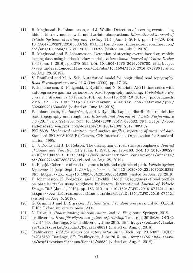
[111] R. Maghsood, P. Johannesson, and J. Wallin. Detection of steering events usinghidden Markov models with multivariate observations. International Journal ofVehicle Systems Modelling and Testing 11.4 (Jan. 1, 2016), pp. 313–329. doi:10.1504/IJVSMT.2016.083752. url: https://www.inderscienceonline.com/doi/abs/10.1504/IJVSMT.2016.083752 (visited on July 9, 2018).

[112] R. Maghsood and P. Johannesson. Detection of steering events based on vehiclelogging data using hidden Markov models. International Journal of Vehicle Design70.3 (Jan. 1, 2016), pp. 278–295. doi: 10.1504/IJVD.2016.075780. url: https://www.inderscienceonline.com/doi/abs/10.1504/IJVD.2016.075780 (visitedon Aug. 28, 2019).

[113] V. Rouillard and M. A. Sek. A statistical model for longitudinal road topography.Road & transport research 11.3 (Oct. 2002), pp. 17–23.

[114] P. Johannesson, K. Podgorski, I. Rychlik, and N. Shariati. AR(1) time series withautoregressive gamma variance for road topography modeling. Probabilistic En-gineering Mechanics 43 (Jan. 2016), pp. 106–116. doi: 10.1016/j.probengmech.2015 . 12 . 006. url: http : / / linkinghub . elsevier . com / retrieve / pii /

S0266892015300655 (visited on June 18, 2018).[115] P. Johannesson, K. Podgzorski, and I. Rychlik. Laplace distribution models for

road topography and roughness. International Journal of Vehicle Performance3.3 (2017), pp. 224–258. doi: 10.1504/IJVP.2017.085032. url: https://www.inderscienceonline.com/doi/abs/10.1504/IJVP.2017.085032.

[116] ISO 8608. Mechanical vibration, road surface profiles, reporting of measured data.Standard ISO 8608:1995(E). Geneva, CH: International Organization for Standard-ization, 1995.

[117] C. J. Dodds and J. D. Robson. The description of road surface roughness. Journalof Sound and Vibration 31.2 (Jan. 1, 1973), pp. 175–183. doi: 10.1016/S0022-460X(73)80373-6. url: http://www.sciencedirect.com/science/article/pii/S0022460X73803736 (visited on Aug. 28, 2019).

[118] K. Bogsjo. Coherence of road roughness in left and right wheel-path. Vehicle SystemDynamics 46 (sup1 Sept. 1, 2008), pp. 599–609. doi: 10.1080/00423110802018289.url: https://doi.org/10.1080/00423110802018289 (visited on Aug. 28, 2019).

[119] P. Johannesson, K. Podgorski, and I. Rychlik. Modelling roughness of road profileson parallel tracks using roughness indicators. International Journal of VehicleDesign 70.2 (Jan. 1, 2016), pp. 183–210. doi: 10.1504/IJVD.2016.074421. url:https://www.inderscienceonline.com/doi/abs/10.1504/IJVD.2016.074421

(visited on Aug. 5, 2018).[120] G. Grimmett and D. Stirzaker. Probability and random processes. 3rd ed. Oxford,

U.K.: Oxford university press, 2001.[121] N. Privault. Understanding Markov chains. 2nd ed. Singapore: Springer, 2018.[122] Trafikverket. Krav for vagars och gators utformning. Tech. rep. 2015:086. OCLC:

942315330. Borlange, SE: Trafikverket, June 2015. url: http://online4.ineko.se/trafikverket/Product/Detail/48631 (visited on Aug. 6, 2018).

[123] Trafikverket. Rad for vagars och gators utformning. Tech. rep. 2015:087. OCLC:942315159. Borlange, SE: Trafikverket, June 2015. url: http://online4.ineko.se/trafikverket/Product/Detail/48632 (visited on Aug. 6, 2018).

71


https://www.inderscienceonline.com/doi/abs/10.1504/IJVSMT.2016.083752

https://www.inderscienceonline.com/doi/abs/10.1504/IJVSMT.2016.083752




https://doi.org/10.1016/j.probengmech.2015.12.006

https://doi.org/10.1016/j.probengmech.2015.12.006

http://linkinghub.elsevier.com/retrieve/pii/S0266892015300655

http://linkinghub.elsevier.com/retrieve/pii/S0266892015300655

https://doi.org/10.1504/IJVP.2017.085032

https://www.inderscienceonline.com/doi/abs/10.1504/IJVP.2017.085032

https://www.inderscienceonline.com/doi/abs/10.1504/IJVP.2017.085032

https://doi.org/10.1016/S0022-460X(73)80373-6

https://doi.org/10.1016/S0022-460X(73)80373-6

http://www.sciencedirect.com/science/article/pii/S0022460X73803736

http://www.sciencedirect.com/science/article/pii/S0022460X73803736

https://doi.org/10.1080/00423110802018289

https://doi.org/10.1080/00423110802018289



http://online4.ineko.se/trafikverket/Product/Detail/48631




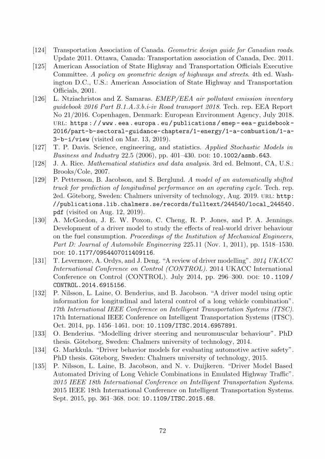
[124] Transportation Association of Canada. Geometric design guide for Canadian roads.Update 2011. Ottawa, Canada: Transportation association of Canada, Dec. 2011.

[125] American Association of State Highway and Transportation Officials ExecutiveCommittee. A policy on geometric design of highways and streets. 4th ed. Wash-ington D.C., U.S.: American Association of State Highway and TransportationOfficials, 2001.

[126] L. Ntziachristos and Z. Samaras. EMEP/EEA air pollutant emission inventoryguidebook 2016 Part B.1.A.3.b.i-iv Road transport 2018. Tech. rep. EEA ReportNo 21/2016. Copenhagen, Denmark: European Environment Agency, July 2018.url: https://www.eea.europa.eu/publications/emep- eea- guidebook-

2016/part-b-sectoral-guidance-chapters/1-energy/1-a-combustion/1-a-

3-b-i/view (visited on Mar. 13, 2019).[127] T. P. Davis. Science, engineering, and statistics. Applied Stochastic Models in

Business and Industry 22.5 (2006), pp. 401–430. doi: 10.1002/asmb.643.[128] J. A. Rice. Mathematical statistics and data analysis. 3rd ed. Belmont, CA, U.S.:

Brooks/Cole, 2007.[129] P. Pettersson, B. Jacobson, and S. Berglund. A model of an automatically shifted

truck for prediction of longitudinal performance on an operating cycle. Tech. rep.2ed. Goteborg, Sweden: Chalmers university of technology, Aug. 2019. url: http://publications.lib.chalmers.se/records/fulltext/244540/local_244540.

pdf (visited on Aug. 12, 2019).[130] A. McGordon, J. E. W. Poxon, C. Cheng, R. P. Jones, and P. A. Jennings.

Development of a driver model to study the effects of real-world driver behaviouron the fuel consumption. Proceedings of the Institution of Mechanical Engineers,Part D: Journal of Automobile Engineering 225.11 (Nov. 1, 2011), pp. 1518–1530.doi: 10.1177/0954407011409116.

[131] T. Levermore, A. Ordys, and J. Deng. “A review of driver modelling”. 2014 UKACCInternational Conference on Control (CONTROL). 2014 UKACC InternationalConference on Control (CONTROL). July 2014, pp. 296–300. doi: 10.1109/CONTROL.2014.6915156.

[132] P. Nilsson, L. Laine, O. Benderius, and B. Jacobson. “A driver model using opticinformation for longitudinal and lateral control of a long vehicle combination”.17th International IEEE Conference on Intelligent Transportation Systems (ITSC).17th International IEEE Conference on Intelligent Transportation Systems (ITSC).Oct. 2014, pp. 1456–1461. doi: 10.1109/ITSC.2014.6957891.

[133] O. Benderius. “Modelling driver steering and neuromuscular behaviour”. PhDthesis. Goteborg, Sweden: Chalmers university of technology, 2014.

[134] G. Markkula. “Driver behavior models for evaluating automotive active safety”.PhD thesis. Goteborg, Sweden: Chalmers university of technology, 2015.

[135] P. Nilsson, L. Laine, B. Jacobson, and N. v. Duijkeren. “Driver Model BasedAutomated Driving of Long Vehicle Combinations in Emulated Highway Traffic”.2015 IEEE 18th International Conference on Intelligent Transportation Systems.2015 IEEE 18th International Conference on Intelligent Transportation Systems.Sept. 2015, pp. 361–368. doi: 10.1109/ITSC.2015.68.

72

https://www.eea.europa.eu/publications/emep-eea-guidebook-2016/part-b-sectoral-guidance-chapters/1-energy/1-a-combustion/1-a-3-b-i/view



https://doi.org/10.1002/asmb.643

http://publications.lib.chalmers.se/records/fulltext/244540/local_244540.pdf



https://doi.org/10.1177/0954407011409116

https://doi.org/10.1109/CONTROL.2014.6915156

https://doi.org/10.1109/CONTROL.2014.6915156



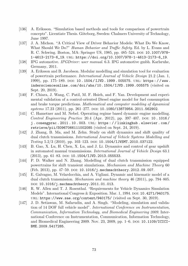
[136] A. Eriksson. “Simulation based methods and tools for comparison of powertrainconcepts”. Licentiate Thesis. Goteborg, Sweden: Chalmers University of Technology,June 1997.

[137] J. A. Michon. “A Critical View of Driver Behavior Models: What Do We Know,What Should We Do?” Human Behavior and Traffic Safety. Ed. by L. Evans andR. C. Schwing. Boston, MA: Springer US, 1985, pp. 485–524. doi: 10.1007/978-1-4613-2173-6_19. url: https://doi.org/10.1007/978-1-4613-2173-6_19.

[138] IPG automotive. IPGDriver: user manual. 6.3. IPG automotive gmbh. Karlsruhe,Germany, 2011.

[139] A. Eriksson and B. Jacobson. Modular modelling and simulation tool for evaluationof powertrain performance. International Journal of Vehicle Design 21.2 (Jan. 1,1999), pp. 175–189. doi: 10.1504/IJVD.1999.005575. url: https://www.

inderscienceonline.com/doi/abs/10.1504/IJVD.1999.005575 (visited onSept. 20, 2019).

[140] F. Chiara, J. Wang, C. Patil, M. F. Hsieh, and F. Yan. Development and experi-mental validation of a control-oriented Diesel engine model for fuel consumptionand brake torque predictions. Mathematical and computer modeling of dynamicalsystems 17.23 (2011), pp. 261–277. doi: 10.1080/13873954.2011.562902.

[141] C. Hametner and M. Nebel. Operating regime based dynamic engine modelling.Control Engineering Practice 20.4 (Apr. 2012), pp. 397–407. doi: 10 . 1016 /

j . conengprac . 2011 . 10 . 003. url: https : / / linkinghub . elsevier . com /

retrieve/pii/S0967066111002085 (visited on Sept. 24, 2019).[142] J. Zhang, B. Ma, and M. Zehn. Study on shift dynamics and shift quality of

dual clutch transmissions. International Journal of Vehicle Systems Modelling andTesting 5.2/3 (2010), pp. 103–123. doi: 10.1504/IJVSMT.2010.037122.

[143] B. Gao, X. Lu, H. Chen, X. Lu, and J. Li. Dynamics and control of gear upshiftin automated manual transmissions. International Journal of Vehicle Design 63.1(2013), pp. 61–83. doi: 10.1504/IJVD.2013.055533.

[144] P. D. Walker and N. Zhang. Modelling of dual clutch transmission equippedpowertrains for shift transient simulations. Mechanism and Machine Theory 60(Feb. 2013), pp. 47–59. doi: 10.1016/j.mechmachtheory.2012.09.007.

[145] E. Galvagno, M. Velardocchia, and A. Vigliani. Dynamic and kinematic model of adual clutch transmission. Mechanism and machine theory 46 (2011), pp. 794–805.doi: 10.1016/j.mechmachtheory.2011.01.013.

[146] R. W. Allen and T. J. Rosenthal. “Requirements for Vehicle Dynamics SimulationModels”. International Congress & Exposition. Mar. 1, 1994. doi: 10.4271/940175.url: https://www.sae.org/content/940175/ (visited on Sept. 30, 2019).

[147] J. D. Setiawan, M. Safarudin, and A. Singh. “Modeling, simulation and valida-tion of 14 DOF full vehicle model”. International Conference on Instrumentation,Communication, Information Technology, and Biomedical Engineering 2009. Inter-national Conference on Instrumentation, Communication, Information Technology,and Biomedical Engineering 2009. Nov. 23, 2009, pp. 1–6. doi: 10.1109/ICICI-BME.2009.5417285.

73

https://doi.org/10.1007/978-1-4613-2173-6_19

https://doi.org/10.1007/978-1-4613-2173-6_19

https://doi.org/10.1007/978-1-4613-2173-6_19




https://doi.org/10.1080/13873954.2011.562902

https://doi.org/10.1016/j.conengprac.2011.10.003

https://doi.org/10.1016/j.conengprac.2011.10.003





https://doi.org/10.1016/j.mechmachtheory.2012.09.007

https://doi.org/10.1016/j.mechmachtheory.2011.01.013

https://doi.org/10.4271/940175

https://www.sae.org/content/940175/

https://doi.org/10.1109/ICICI-BME.2009.5417285

https://doi.org/10.1109/ICICI-BME.2009.5417285

[148] S. Sedran, F. Bruzelius, S. Kharrazi, B. Jacobson, and N. Amati. “A heavy vehicledynamics model for driving simulators”. 14th International Symposium on HeavyVehicle Transport Technology (HVTT14). Rotorua, New Zealand, Nov. 2016.

[149] M. Dupuis, M. Strobl, and H. Grezlikowski. “OpenDRIVE 2010 and beyond -status and future of the de facto standard for the description of road networks”.Driving simulation conference Europe 2010. Paris, France, Sept. 2010.

74

Documents

Operating cycle representations for road vehicles