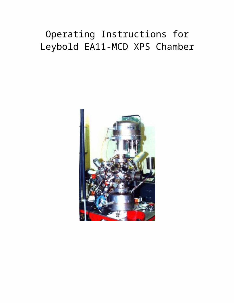
Operating Instructions for Leybold EA11-MCD XPS Chamber

Updates: Nathan Havercroft on April 30 2001

Hugo Tiznado on April 08 2005

Table of Contents

Table of Contents.................................................................................................................2Table of Figures...................................................................................................................4Electronic Units...................................................................................................................5Vacuum System...................................................................................................................6

Evacuating the Instrument...............................................................................................6Venting the Instrument....................................................................................................7UHV Bake-Out................................................................................................................7

X-ray Source........................................................................................................................7Initial Operation...............................................................................................................8Turning on the X-rays......................................................................................................9Turning off the X-rays.....................................................................................................9Maintenance.....................................................................................................................9

Replacing the Anode....................................................................................................9Replacing the Filament (Cathode).............................................................................10Replacing the Aluminum Window............................................................................10

Detector System.................................................................................................................11Multi Channel Plates (MCP).........................................................................................11

Servicing the detector system....................................................................................11Using the SPECTRA software...........................................................................................12

Setting up the data acquisition card...............................................................................12Collecting an XPS spectrum..........................................................................................13Analyzing XPS Data......................................................................................................13

Tools Window...........................................................................................................14Background Subtraction............................................................................................15Curve Fitting..............................................................................................................15Quantification............................................................................................................16Difference Spectra.....................................................................................................16Calibration.................................................................................................................17Adding Labels............................................................................................................17

Testing the Analyzer..........................................................................................................17Flood Gun..........................................................................................................................18

Operation.......................................................................................................................18PHI Ion Gun.......................................................................................................................18

Turning on the Ion Gun.................................................................................................18Turning off the Ion Gun.................................................................................................19

Mass Spectrometer.............................................................................................................19Turning on the MS.........................................................................................................19Standby Mode................................................................................................................19Turning off the MS........................................................................................................20Software.........................................................................................................................20

Collecting a mass spectrum using SPECTRA...........................................................20Collecting a spectra using SIMS6R...........................................................................21Collecting a single spectra using BASICA................................................................22

2

Contacts.............................................................................................................................22Dietrich von Diemar..................................................................................................22Ron Unwin.................................................................................................................22Tim Cotter..................................................................................................................22

3

Table of FiguresFigure 1 Photograph of the electronic units.........................................................................5Figure 2 X-ray Source.........................................................................................................8Figure 3 The Tools Window..............................................................................................15Figure 4 The Peak List Window........................................................................................16Figure 5 A Typical Label...................................................................................................17

4

Electronic Units

Figure 1 Photograph of the electronic units

Key:1. Ionivac IM510 Ionization Gauge located in preparation chamber.2. Granville Phillips 271 Ionization Gauge located in analysis chamber.3. Thermovac TM230 Gauge located in preparation chamber and load-lock

pump/backing lines.4. Bake-out Control (861915) inc. Thermovac TM210 located in analysis chamber

backing line.5. UTI 100C precision mass analyzer6. Power Control Unit (861900)7. Turbotronik NT150/360 for preparation chamber turbo pump.8. Turbotronik NT450 for analysis chamber turbo pump.9. Flood gun power supply (869900)10. Ion gun power supply (867911) (ion gun located in preparation chamber)

5

11. PHI ion gun 20-115 located in analysis chamber. (No longer on this instrument)12. Emission regulation X-ray source (865920)13. High voltage supply (865925)14. Cooling water isolation box (865929)15. Multiplier supply (865976)16. Multiplier supply (865976)17. HV amplifier bipolar 86597818. Energy analyzer power supply PS-EA11N (865903)19. Data acquisition unit (865985)20. Sample lock drive unit (862914)21. MCD power filter unit22. Transformer 110/220 (861905)

Items not numbered are not labeled; however the Hans Knürr units are cooling fans for the electronics.

Vacuum System

Evacuating the InstrumentIf the chamber is at atmospheric pressure for whatever reason the following are the necessary steps to obtain ultra-high vacuum.

1. Make sure all valves are closed to atmosphere and all seals are tight2. Ensure that the cooling water is flowing to the turbo pumps with a pressure of at

least 3 lpm3. On the Power Control Unit (861900) turn pump groups A and B on4. Ensure the valves between the backing and the turbo pumps are open, there is one

valve per turbo pump5. Turn on the low vacuum gauges labeled analysis (Thermovac TM210 situated on

the Bake-out Control Unit 861915) and preparation chamber (Thermovac TM230)6. Turn on the two backing pumps7. Allow the pressure to decrease in to the 10-2 Torr range8. Turn on the two turbo pumps by pressing the start buttons on both turbo pump

control panels9. After 30 minutes or when the pressure on the low vacuum gauges is in the 10-3

range turn on the two ionization gauges by pressing the power on followed by the filament emission

a. Granville Phillips 271 unit in analysis chamberb. Leybold Ionivac IM510 unit in preparation chamber

10. Pressure should fall steadily to 10-6-10-7 Torr in the preparation chamber and 10-8 –10-9 Torr in the analysis chamber

6

Venting the InstrumentThere may be situations where the chamber needs to be vented, such as to replace a filament in the X-ray source. To do this you should,

1. Ensure all HV sources are switched off2. Turn off all ionization gauges3. Open the Nitrogen flow4. Turn off the pump groups A and B buttons5. Open the vent valves bellow the turbo pumps slowly so as not to blow the X-ray

window

UHV Bake-Out1. Ensure the chamber has good vacuum2. Remove all non bake-able cables3. Detach water cooling lines and HV from X-ray gun4. Blow residual cooling water out of the anode with compressed air5. Ensure all bake out lines are correctly attached6. The X-ray bypass switch should be in the interlock position7. Set the trigger level on the TM 210 S to the desired vacuum8. Select the bake out temperature by pressing in the central button and rotating dial

(0 – 450 °C) generally 150 °C9. Set timer to the desired time (0 – 60 hours) generally 8 hours10. On the temperature dial both the red and white lights will become lit, the red lamp

will extinguish when the desired temperature has been reached. This light shows when the heater is on

11. The blue X-ray by pass should illuminate as should the green timer light12. After bake out allow to cool and reassemble in reverse order

X-ray SourceThe X-ray source is specifically designed for use with X-ray photoelectron spectroscopy (XPS) systems and is fitted with a dual source anode, magnesium (1253.6 eV) and aluminum (1486.6 eV). This allows easy switching between the sources and therefore rapid distinction between photoelectron and Auger peaks and linear scale calibration.

7

Figure 2 X-ray Source

Initial OperationWhen using the X-ray source for the first time after it has been at atmospheric pressure for example after changing the anode, filaments or aluminum window it is necessary to use the following procedures.

1. Check all connections are correct2. Vacuum should be lower than 1x10-5 Torr3. Ensure HV dial is fully counter clockwise on the HV Supply Unit (865925)4. Ensure Emission Regulator is set to “stand by” on Emission Regulation Unit

(865920)5. Turn on the cooling water at a pressure of about 3.5 – 4.0 lpm6. On the Power Control Unit urn the Main Switch Key to ON and Press the

Electronics button to ON7. On the HV unit press the water on button8. When the water light is lit press the HV button9. Turn HV to 8kV and leave for 45 – 60 minutes10. Slowly increase to desired value (<14 kV)11. On the Emission Regulation Unit choose the desired anode12. Turn the emission dial to the desired value13. Turn on the Emission Regulation Unit14. Leave for 10 minutes to degas15. Switch from “stand by” to “operate”

The displayed emission current could be about 2 or 3 mA greater than the value set on the Emission Regulation Unit due to current leakage through the water supply.

Note: If in the “operate” mode the “current limit” lamp is on then the HV chosen is not sufficient to support the current. Immediately increase the voltage or decrease the current in order to maintain the life of the filament. Also the “stand by/operate” switch is temperamental so insure that the switch has indeed been moved, by monitoring the current dial.

8

Turning on the X-raysThe following procedure assumes that the source has been operated previously with its current anode, filaments and x-ray window. If not please follow the procedure above, “Initial Operation”.

1. Check all connections are correct2. Vacuum should be lower than 1x10-5 Torr3. Ensure HV dial is fully counter clockwise4. Turn on the Emission Regulation Unit5. On the Emission Regulation Unit choose the desired anode6. Turn the emission dial to the desired value7. Ensure Emission Regulator is set to “stand by”8. Turn on the cooling water at a pressure of about 3.5 – 4.0 lpm9. On the Power Control Unit (861900) turn on the main switch by rotating the key

if necessary10. Press the electronics on button on the same unit11. On the HV unit press the water on button12. When the water light is lit press the HV button13. Increase the HV to the desired value by rotating the large dial14. Switch from “stand by” to “operate”

The displayed emission current may be about 2 or 3 mA greater than the value set on the Emission Regulation Unit due to current leakage through the water supply.

Note: If in the “operate” mode the “current limit” lamp is on then the HV chosen is not sufficient to support the current. Immediately increase the voltage or decrease the current in order to maintain the life of the filament.

Turning off the X-rays1. Turn Emission Regulation Unit to “stand by”2. Turn High voltage dial completely counter clockwise3. Switch off HV by pressing “HV off” button4. Press “Water off” button5. Turn water supply off (only to X-ray source)

Note: If for some reason the HV is automatically switched off the above procedure should be carried out before the HV is switched on again

Maintenance

Replacing the AnodeTechnically this can be done without removing the entire X-ray source from the chamber, however due to alignment issues it is best to remove the source from the chamber

1. Remove the external connections as described in the “Bake-Out” section

9

2. Vent the chamber as described above in “Venting the Instrument”3. Remove the source from the chamber by undoing the 4½” flange (½” bolts)4. Loosen the end cap screws (M6) and gently pull off the end cap5. Remove the screws on the 2¾” CF water inlet flange of the anode6. Remove the water cooling tube from inside the anode7. Remove the anode8. Replace anode and all copper gaskets including the water sealing ring before

replacing the cooling water tube9. Tighten screws so that anode is perfectly centered10. Screw the end cap in place and check the connectivity of the filaments before

placing in the vacuum

Replacing the Filament (Cathode)1. Remove the external connections as described in the “Bake-Out” section2. Vent the chamber as described above in “Venting the Instrument”3. Remove the source from the chamber by undoing the 4½” CF flange (½” bolts)4. Loosen the end cap screws (M6) and gently pull off the end cap5. Undo the 4 fixing grub (set) screws and pull off the old filament6. Place the new spiral tungsten filament on the supporting pins and slide down until

the upper part of the filament is level with the surface of the anode.7. Tighten the 4 fixing grub (set) screws8. Replace the end cap being sure that it does not touch either of the filaments.9. Screw the end cap in place and check the connectivity of the filaments before

placing in the vacuum

Replacing the Aluminum Window1. Remove the external connections as described in the “Bake-Out” section2. Vent the chamber as described above in “Venting the Instrument”3. Remove the source from the chamber by undoing the 4½” flange (½” bolts)4. Unscrew the window from the end cap5. Gently slide out the window6. Remove aluminum foil by gently scraping and rubbing with iso-propanol7. Clean the metallic plate with iso-propanol8. Cut a new piece of 2μm foil (99.1%) to approximately the correct size9. Fix the new window to the metallic plate with a small amount of colloidal

graphite10. Allow to dry11. Trim off excess aluminum foil12. Carefully replace the window into the groove and screw into place13. Check the connectivity of the filaments before placing in the vacuum

10

Detector SystemThe Leybold system is fitted with a Leybold EA11 MCD hemispherical electrostatic energy analyzer, which allows the measurement of positive and negative particles with kinetic energies ranging from 0 to 2.6keV. The analyzer is equipped with an 18-channel detector system that is bake-able up to 150°C. It is also equipped with a variable slit mechanism for a selectable acceptance area and a tilt mechanism for better alignment of point/line sources such as AES, SAM, ISS and monochromatic XPS.

Multi Channel Plates (MCP)An MCP is an array of millions of single channel multipliers fused together in a precision matrix. It is made from lead-doped glass and typically has channel walls of about one micron thick. The MCP’s should always be handled by their solid glass border and it is very important that they should be kept under vacuum at all times. Extended exposure to atmospheric conditions can lead to early degradation of the plates.

Servicing the detector systemMulti channel plates should be considered a consumable item, as over a period of time they will lose their gain ability. When a significant change in performance is noticed they should be changed. The SPECS EA11MCD users manual (page 38) should be consulted when changing the plates but below is a synopsis of the procedure. Care should be taken to remember exactly where all connections and parts are situated.

1. Remove the MCD pre-amplifier and coupling box2. Vent the system as described previously3. Remove the analyzer vacuum hood and mu metal shielding taking care to note

their orientation and the position of the spacers on the lens side of the mu metal shielding

4. Disconnect the electrical connections to the outer hemisphere5. Unscrew the outer hemisphere from the ground plate and remove it carefully6. Unscrew the slit mechanism from it’s ceramic holder7. If necessary remove the 20 pin lens feed-through and the 6pin MCD feed-through

(this may not be necessary to remove the hemispheres but it will be necessary to remount them)

8. Remove the four springs9. Remove the two screws around the exit grid, this will detach the MCD from the

ground plate10. If the hemispheres and lens system needs to be removed the outer hemisphere

should be reattached and then the whole assembly lifted from the chamber. Note: this is very heavy and two people will be needed for this task.

11. If the MCP’s are replaced care should be taken to ensure they are replaced in the correct orientation with the marks aligned opposite each other.

12. The MCP labeled “output” should be placed on the bottom and the one labeled “input” should be positioned on the top

11

13. As stated above the 20pin lens feed-through and the 20pin detector feed-through (if the MCD has been removed) will need to be removed before the hemisphere and lens assembly is replaced

14. Once the hemispheres and MCD are back in place these feed-throughs need to be carefully positioned so that all the pins fall completely into the correct hole.

15. Once everything has been replaced and checked for no illegal contacts the system should be evacuated before being tested (see the testing section below)

Using the SPECTRA softwareXPS spectra should be taken using the SPECTRA program on the PC. This suite of programs consists of three parts, COLLECTS, PRESENTS and DATABASE. COLLECTS is used for collecting data, PRESENTS is the data analysis part of the package and DATABASE contains information on peak positions and relative intensities. A comprehensive manual exists for the software however the manual is for version 7 and the software is actually version 8.0E-7 so some differences exist. The full details are,

Version: 8.0E-7Serial number: SP-03-721-20015Hardware type: 1.2.1.0Drive type: SP721-00-I-SPEC

Setting up the data acquisition card1. Boot up the PC if necessary, network password is ea11lmcd and just click cancel

for the windows password2. Double click on the COLLECTS icon on the PC3. Three windows will open up, a COLLETCS screen, a LABBOOK screen and a

window to open a LABBOOK file4. Hit cancel on the open LABBOOK window5. Click on the tools icon which is located in the top right hand corner of the

COLLECTS window, it is the middle of the three and looks like a hammer6. From the available menu select Set Up Card7. A new window will appear with several options, some of the basic options should

be set to,a. Sig Source: 5 (MCD)b. X-max: 1638.4c. Timebase: 0 (10ms)d. Region 10: 0 (normal)e. Excitation: Choose the appropriate source, 1486.6 for Al or 1253.6 for Mgf. To setup the MCD card look to the bottom right hand cornerg. The driver type should be: SPF01xchh. By clicking on Linear the dispersion value can be set to: 0.003968 This

value is very important and should not be changed without consulting the instrument manufacturer

8. The work function can be used to adjust for any linear drift in the axis9. Click on OK to accept all the settings

12

Collecting an XPS spectrumUsing the following procedure a series of spectra can be obtained.

1. Boot up the PC if necessary, network password is ea11lmcd and just click cancel for the windows password

2. On the Power Control Unit urn the Main Switch Key to ON and Press the Electronics button to ON

3. Switch on the EA11N power supply followed by the HV Bipolar amplifier and the multiplier supply

4. Set the multiplier supply to the correct voltage (8.9 scale units at present)5. Ensure that the x-rays are on as described in the turning on the X-rays section

above6. Double click on the COLLECTS icon on the PC7. Three windows will open up, a COLLETCS screen, a LABBOOK screen and a

window to open a LABBOOK file8. Note the lab book allows users to enter comments about the experiment much like

a real lab book9. Either choose the desired LABBOOK or enter a new filename for a new

experiment10. To set up regions to be run click on the Edit Regions/Summary icon which is

situated immediately to the right of the region numbers (1-10)11. This will open a spreadsheet where the region details can be entered12. When finished this screen can be minimized by clicking on the Edit

Regions/Summary icon again13. Note the pass energy is not set by the computer program, you will have to set it on

the PS-EA11N independently14. To choose which regions will be run click on the check boxes above the

appropriate number, regarding item 12 only regions with the same pass energy should be set to run at the same time

15. To start the spectral series click Go16. The data collection can be paused at any time by clicking on Go again and

restarted by clicking again on Go17. When the data has been collected it can be saved by clicking on the appropriate

icon18. Note Only regions with a check mark above them will be saved

Analyzing XPS DataThe XPS data collected using the COLLECTS program can be analyzed using the PRESENTS program. The data can be loaded directly into the program without any modifications or conversions.

PRESENTS contains all of the data reduction features of the SPECTRA program with several important additions : -

o Quantification via editable database.o Copy peak/quantification information to documents via clipboard.o Addition of title and peak labels.

13

o Cursor and peak separation display.o Scalable generation of transferable images (via clipboard/bitmaps).o Twin column (Energy/intensity) text values can be transferred via clipboard to

other programs, e.g. spreadsheets and graphics.o Uniquely powerful on-line graphical help.o Full colour printing support with spectral details.o Data prescaled on file input. o Preservation of region scaling.o Individually lockable and rescaleable X- and Y-axis.o Labbook facility, to aid communications with data collection package. o Region by region charge compensation.

Toolbox features: -o Smoothing (3, 5 point, FFT, Savitzky-Golay and Optimal).o Background (Minimum, Linear, Shirley, Tougaard)o FWHM - peak measurement generating a table of values (primitive

quantification).o Two Curve fitting methods, 8 peaks with Gauss-Lorentz sum and product

function and the ability to use any analytical or non-analytical function.o Spectra feature can be used as curve fit shapes.o Fitting provides statistical evaluation parameters for error estimates.o Update quantification table from peak-fit results.o Tabulation of Standard deviations and fit quality.o De-convolution with measured spectral features as a template. o Differentiation, Integration and De-spiking.o Copy of Peak Fit data to clipboard as Bitmap or text with axis labels.o Plotting of Fit/Quantification results with editable peak colours/fillings.o Plotting of Envelope and residuals from curve fit results.o Automatic peak labeling.o Automatic peak location and tabulation.o Process macros can be stored for repeatable and faster processing.o Transmission function correction by either E**n or rational polynomial

method.o Multi-experiment bulk data reduction (Macro generation).

File processing: - o Multiple TEXT File I/O formats (Standard, VAMAS, E-Y, and E-dE,Y).o Auto detection of simple file formats.o The users own file formats can be included using DLL extensions.o Files can be appended to existing regions.o Selected regions can be deleted.

14

Tools WindowThe tools window contains several icons that are used to perform the majority of data analysis tasks as well as containing a zoom feature. These can be seen below in figure 3.

Figure 3 The Tools Window

Background SubtractionThis is achieved very simply, with the desired spectrum on the screen click on the Background Subtraction icon in the Tools window, and the user chooses the desired type of background. The spectra may disappear from the screen, if this happens simply click on the left arrow key to rescale the screen.

Curve FittingIt is best to remove a linear background using the method described above before starting the curve fitting process. Once the background has been remove click on the Find button in the Tools window, enter the desired options and click OK. A new window labeled Peak List will appear containing the starting parameters for the fit, as shown in figure 4 below. By clicking on the boxes in the column labeled # the starting peaks can be seen. If this process has not found all the relevant peaks the user can add additional peaks by drawing a box with the dimensions and desired location of the peak on the screen and then pressing Alt-N.

Next click on the Curve Fit icon in the Tools window and choose the desired background to be included in the fit (generally Shirley for a narrow region). Right clicking on the relevant boxes can alter the properties of the peaks. These values can be linked to other peaks, for example you can specify that peak 2 should be 1.2eV to lower binding energy than peak 1. To do this enter the following syntax P1+0 where P1 is peak 1 in this case,

15

+ is add and 0 is the amount. Other allowed operators are, – and *, where * signifies a ratio. You cannot use multiple operators in a single cell and you cannot use * when referring to peak position. Double left clicking on the boxes will fix the peak parameter, which is indicated by a red bar inside the box. After choosing which fit method you desire you can then start the fitting process by clicking on the Start Fit button. The procedure will stop when a suitable fit has been found or when the fit crashes, indicated by the green progress bar turning red. If a blue bar appears in one of the Peak Fit Window cells this indicates that the parameter has reached its maximum allowed value and the fit needs changing. Once you have a suitable fit you can click on OK to return you to the main PRESENTS screen. Clicking on the relevant button in the Peak List window will show the envelope of the fit.

Figure 4 The Peak List Window

QuantificationIn order to quantify the elements present, all peaks need to be curve fitted as described in the above section. In order to obtain the concentration percentage (column 2 in the peak list window) you should double click in the Name column for each peak. This will open the database and you should then choose the desired atomic level, e.g. C1s. This will automatically calculate the concentration for all the peaks that have elements assigned to them. Note that the database cannot be opened in PRESENTS if COLLECTS is also running.

Difference SpectraThis is achieved by clicking on the difference spectra icon (diff A-B). Regions can only be added or subtracted over the energy range that they share. A dialogue box will then open and you should input your request in the following syntax,

16

Destination region = region A – region B

Therefore a free region is needed to display the results. Spectra can also be added as well as fractional spectra, e.g.

10 = 1 + 5*0.5

Indicating that region 10 will display the resulting spectra from the addition of region 1 added to half the intensity of region 5.

CalibrationThis is achieved by displaying the desired region (usually C1s for internal calibration against hydrocarbon) and drawing a box from the actual peak location to the desired location then clicking on the calibrate button at the top right of the PRESENTS screen. The user will be asked if all regions or just the one displayed should be shifted by the amount indicated by the box width. Select the desired option and click OK.

Adding LabelsIn order to add a label to a spectra first draw a box whose coordinates will determine the position of the label. By holding down the left mouse button and starting in the bottom left hand corner of the box and releasing the mouse button in the top right hand corner a label such as the one shown in figure 5 can be drawn. Other labels can be drawn by varying the start and end positions of the box. If the selected region is changed then all labels will be lost.

Figure 5 A Typical Label

Testing the AnalyzerAfter any modifications to the analysis system, lenses hemispheres and detector the system should be tested in the following manner.

1. Etch a piece of silver to remove any oxide and contaminants present2. Run the Ag 3d5/2 region and measure the FWHM at a pass energy of 31.5eV it

should be 0.9eV Adjust the multiplier voltage until it is (try 8.4 scale units as a starting point)

17

3. Run the Ag 3d5/2 region at varying pass energies to see of the peak position changes

4. If the position is not independent of pass energy the outer hemisphere voltage needs to be adjusted. This is done by altering the potentiostat for U9

5. Once the voltage has been adjusted so that peak position is independent of pass energy all the voltages should be measured carefully with an HV probe

6. Next change the sample for a copper/gold sample so that the linearity of the scale can be checked

7. Adjust the Gain for the 1.6kV range setting on the HV Bipolar unit until the separation between the Au4f7/2 (84.0eV) and Cu2p3/2 (932.66eV) peaks is correct

8. Once the linearity has been corrected any linear offset can be adjusted with the work function dial on the HV Bipolar unit

Flood GunThe flood gun is used to compensate charge build up on insulated samples by electron bombardment.

Operation1. Ensure the 4-pin plug is connected to the flood gun with the 3 screws; it will only

go one way due to the combination of a 4 fold and 3 fold symmetry.2. Turn the power unit (869900) on3. Set the desired “Electron Energy” 0 to 500 eV4. Set the desired “Electron Current” 0 to 100 μA5. If necessary correct by using the “Extractor Voltage”6. Note: if the electron energy is 0 eV the electron current should be 0μA in order to

preserve the filament life7. To turn off the flood gun repeat steps in reverse order

PHI Ion GunNote this gun has been removed from the chamber for use on the micro reactor chamber.

The PHI ion gun, model 04-191 is controlled by unit 20-115 and is used to etch the sample surface. This is done by, heating a filament, which then emits electrons. These electrons are then attracted to a more positive anode. Some of the electrons collide with inert gas molecules (usually argon), which have been bled into the chamber and thus form ions (Ar+). As the filaments, anode and shield are all biased positive these positive ions are accelerated out of the ion gun and on to the sample. On the way out of the ion gun they pass through deflection plates and are focused by additional optics.

Turning on the Ion Gun1. Make sure the power switch is off and the emission control is turned fully counter

clockwise on the control unit (20-115)2. Backfill the chamber with the desired gas to a pressure of 5x10-5 Torr3. Position sample in front of ion beam4. Turn “Beam Voltage” to 5 kV

18

5. Turn “Beam Voltage” switch to off6. Turn “Raster” switch to off7. Turn power on8. Turn “Focus” control to CAL9. Turn up “Emission Current” to 25 mA (on meter)10. Turn on “Beam Voltage”11. Adjust the “X, Y position” and “Raster” controls as necessary

Turning off the Ion Gun1. Turn the “Beam Voltage” switch off2. Turn the “Emission” control fully counter clockwise3. Turn the “Raster” switch off4. Turn the power switch off

Mass SpectrometerThe following section describes the operation of the UTI 100C Precision Mass Analyzer

Turning on the MS1. Ensure the Emission dial is turned completely counter-clockwise2. Set the range to 10-5 amps, to avoid possible filament burn out3. Make sure the damper dial is turned completely counter clockwise4. Depress the MAN key5. Check if the instrument is in protection mode, there is a little switch on the inside

of the front panel (right hand side). If the switch is to the right the protection mode is on

6. Press ON/STANDBY key, wait for 30 – 45 minutes for the system to reach thermal equilibrium

7. Press MULT8. Press EMISS/(MA) and slowly increase the emission current to 2.00±0.01 mA9. Connect the oscilloscope (x to ramp generator and y to signal out), set the scope

to x,y mode10. Depress the EMISS/(MA) key and press VAR to adjust the sweep rate with the

knob on the left hand side. The display over the range gives intensity where as the one over EMISS/(MA) shows mass

11. The scan width and scan center can be adjusted while the EMISS/(MA) button is depressed and WIDTH or MAN are pressed

Standby ModeSwitch the instrument in to standby mode if the instrument will be re-used in a relatively short amount of time, e.g. same day.

1. Place the instrument in TOTAL PRESSURE mode2. Set the range to 10-5 amps3. Make sure that the emission switch is on4. Turn emission dial fully counter clockwise but not off

19

Turning off the MS1. Place the instrument in FARADAY CUP mode2. Set the range to 10-5 amps3. Turn the emission dial off4. Turn the EMISS/(MA) switch off5. Press ON/STANDBY6. Press OFF

Software

Collecting a mass spectrum using SPECTRASetting up the data acquisition cardThis is done in the same manner as described under the XPS section

1. Boot up the PC if necessary, network password is ea11lmcd and just click cancel for the windows password

2. Double click on the COLLECTS icon on the PC3. Three windows will open up, a COLLETCS screen, a LABBOOK screen and a

window to open a LABBOOK file4. Hit cancel on the open LABBOOK window5. Click on the tools icon which is located in the top right hand corner of the

COLLECTS window, it is the middle of the three and looks like a hammer6. From the available menu select Set Up Card7. A new window will appear with several options, some of the basic options should

be set to,a. Sig Source: 3 (Voltage 1)b. X-max: 300 (for Jeff G unit)c. Region 10: 0 (normal)

8. The work function can be used to adjust for any linear drift in the axis (usually 1.0 for the MS)

9. Click on OK to accept all the settings

Collecting a Mass spectrumUsing the following procedure a series of spectra can be obtained in a very similar manner to collecting an XPS spectrum.

1. Boot up the PC if necessary, network password is ea11lmcd and just click cancel for the windows password

2. Switch on the Mass Spectrometer as described above3. Make sure the MS unit is in the EXT mode with the Damper dial set between 9

and 11 o’clock4. Double click on the COLLECTS icon on the PC5. Three windows will open up, a COLLETCS screen, a LABBOOK screen and a

window to open a LABBOOK file6. Note the lab book allows users to enter comments about the experiment much like

a real lab book

20

7. Either choose the desired LABBOOK or enter a new filename for a new experiment

8. To set up regions to be run click on the Edit Regions/Summary icon which is situated immediately to the right of the region numbers (1-10)

9. This will open a spreadsheet where the region details can be entered10. Enter a start and end mass, the step size and dwell time11. When finished this screen can be minimized by clicking on the Edit

Regions/Summary icon again12. Note the computer program does not use the pass energy13. To choose which regions will be run, click on the check boxes above the

appropriate number14. To start the spectral series click Go15. The data collection can be paused at any time by clicking on Go again, to restart

the collection click on Go16. When the data has been collected, it can be saved by clicking on the appropriate

icon 17. Note Only regions with a check mark above them will be saved

Collecting a spectra using SIMS6RNote this software has not been tested with the new acquisition card; it was designed to be used with the old SPECTRA data acquisition card, of which there are none in the lab.

1. Make sure the MS unit is on and in the EXT mode with the Damper dial set to between 9 and 11 o’clock

2. Double click on the SIMS6R icon to launch the program3. After pressing any key to access the program the configuration should be set as,

a. Source – VFC1b. X-max – X=300 (for Jeff G unit)c. Mode – Normal. The integrate mode allows you to follow the

concentration of set masses over time4. Click on “Set” at the top of the screen5. Ten default regions are displayed, which can be edited by clicking on the desired

region, and typing the new value followed by pressing enter.6. Once the regions have been edited the spectra to be collected can be selected by

clicking on the requisite number (it will turn green) and then clicking on exit. More than one region can be selected at once

7. This will bring you back to the spectra acquisition screen8. Press F6 to begin collecting data9. After the data has finished pressing F7 will allow you to name your file and add

comments10. F8 will save the file

21

Collecting a single spectra using BASICANote this software is not currently installed on the computer and is designed for use with and Advantech data acquisition card. Successful use of this software and card on this computer has not been obtained.

1. Open an MS-DOS window 2. Go to the c:\mas directory3. Type basica mspect6 to run the mspect6 software4. Enter the desired values in the program, remembering to switch the mass spec to

EXT and turn the damper to 9 o’clock before running5. Two files will be saved, *.dms and *.ims, the first being the data and the later

being the sample information

ContactsDietrich von DiemarSPECS USA635 South Orange AvenueSarasota, FL 34236Tel: (941) 362-4877Fax: (941) 364-9706Email: didi@specs.com

Ron UnwinSPECTRA softwareEmail: PC_SPECTRA@compuserve.com

Tim CotterVacuum Technology Inc. (UTI Mass Spec)Tel: (865) 481-3342Fax: (865) 481-3788Email: tcotter@vacuumtechnology.com

Andreas Hupfer (last visit to Riverside on March/7-16/2005)hupfer@specs.de

22

Update after the visit of Dr. Andreas Hupfer hupfer@specs.de to UCR on March/7-16/2005.Hugo Tiznado.A summary of the work done:

1. The Al window for the X-rays source was replaced.2. The anodes were cleaned with a glass fiber brush.3. The filament for the Mg anode was replaced because of bad contact.4. The PS EA 11N was recalibrated to have constant kinetic energy position vs.

different pass energies.5. The HV preamplifier was recalibrated to ensure linearity along the energy scale. 6. New work function for the instrument: 5.15 scale units. 7. The maximum of the multiplier voltage was increased from 2.2 to 2.6 kV.8. The “voltage limitation” threshold value in Emission Controller was increased a

little. 9. Some manual files were handed over as *.pdf files.10. The intensity value is now approx. 50% of the designed intensity for a new

analyzer and new anode.11. A scheme of electrical connections can be found in the “XPS Leybold electrical

connections.ppt” file (power point format).

The steps to calibrate the Electron Analyzer system are:

1. Alignment of lenses to increase the counts.a. Introduce a silver foil in the main chamber and clean with the Ar ion gun

until get a reasonable clean survey spectrum (pass energy= 100.8 eV).b. Select the Mg anode and set 20 mA/10kv in the x-rays source filament. In

the “Collects” program choose Processing tools>setup card> MCD>Histogram. Look for the Ag 3d 5/2 peak kinetic energy.

c. It is recommended to take several spectra for both Ag 3d peaks at various pass energies, say 100.8, 63, 31.5 and 15.75 eV (multiples of 3.15), all with step= 0.025 eV. This is useful to see: the shape and change in position of peaks, and compare them after recalibration.

d. (Optional) Open the aperture micrometer to maximum. The counts will go up.

e. Play with the lenses micrometer until get the maximum counts.2. Calibrate the PS EA-11N to have constant kinetic energy position vs. pass

energy and to have symmetrical peaks. More info in page 27 of the Energy Spectrometer EA11 MD manual.

a. Bring out the EA-11N from the rack and open the top cover, keeping all cables and power of the back connected.

b. Set the multiplier voltage to 0 scale units, X-rays off, Work function dial= 0 scale units and pass energy to 100 eV.

c. Short the “Sweep In” BNC connector (ground to live, see picture) in he back of the HV preamplifier.

23

d. Attach the High Voltage probe to a multimeter. Attach the ground of the probe to the ground # 12 in the board of the EA-11N controller.

Ground #12

e. With the probe check the voltages in the terminals and adjust to the values in the next table using the corresponding potentiometers in the board:

Terminal Voltage for KE=0 (sweep in shorted)

Voltages for KE= 198

U11 (Lens 1) 0 -137U10 (inner hemisphere) +128 -69U10’ +108 -88U8 +99 -97U9’ +92 -104U7 +84 -112U9 (outer hemisphere) +72 -124U7’ +14 -183U2 +395 +198

f. Collect a spectrum at pass E= 100.8 and other at 31.5 eV, step 0.025 eV. The position of peaks should be the same, otherwise adjust by turning of the potentiometers U9 and U10 in opposite directions. At this point the

24

peak position should be independent of the pass energy, also they should be symmetric.

3. Calibrate the HV preamplifier to have a linear energy scale. This requires a Gold/Cupper sample. More info in page 26 of the Energy Spectrometer EA11 MD manual.

a. Introduce the sample and clean it by Ar sputtering.b. Collect a spectrum: Pass E= 31.5 eV. The difference for Au 4f7/2 and Cu

2p3/2 peaks should be 848.7+-1 eV. If that is not the case, adjust by the potentiometer for “1.6” in the front panel (move 1/10 or less of turn at time). If the difference is less than 848.7 eV, move the potentiometer counterclockwise.

c. Adjust the dial for Work Function (that is zeroed at this moment), to bring the peaks to the right position.

25

GENERAL NOTES.The Multiplier supply controller (865-976) voltage was increased from 2.2 to 2.6 kV by means of a set of resistors (~ 3 Megaohms) placed in parallel. To check the voltages applied to the MCD, put the high voltage probe indicated in the picture.

26

INSTRUCTIONS FOR DISASSEMBLING ANALYZER

7.2.3.1 Removing the MCD flange Remove the MCD Preamplifier (PA-MCD) and the MCD supply box (SB-MCD).

Vent the system. Open the DN 350 CF flange (remove the screws) and remove the vacuum hood.

Remove the magnetic shielding hood (remove the 3 metal clips before removing the shield).

27

Unscrew four screws connecting the hemispheres.

Disconnect the electrical connections to the outer hemisphere. Remove the ceramic isolation tube that will come out from the screw.

28

Mount the handle to the outer hemisphere and remove it carefully. Take care of the small ceramic plates after remove the hemisphere.

Loosen the slit width mechanism.

29

Remove the 20-pins HAS/lens feedthrough, if necessary.

Disconnect the 6-pin feedthrough from the MCD assembly.

30

Remove the four sticking springs.

Loosen and remove the two screws on the exit grid sheet around the exit grid.

31

Remove the analyzer and put it carefully on a table.

7.2.3.2Changing the MCP Loosen in turn four screws on the MCD head and remove them together with

four metal clips. Remove the top contact ring. Note the orientation key of the top MCP. Remove the top MCP (12 o’clock).

32

Remove the ring between the MCP’s.

Remove the bottom MCP.

33

Unpack the new MCP named “output” (this is the bottom MCP).

Orient the new MCP as the bottom old one (with the orientation key – the arrow head- above and away from the sphere centre –at 6 o’clock-) and put it in place.

Place back the ring between the MCP’s. Unpack the second new MCP named “input”. Orient the second new MCP as the top old one (with the orientation key above

and towards the sphere centre –at 12 o’clock-) and put it in place. Put in the top contact ring. Check the MCP’s on being properly centered. Put four screws together with four metal clips and the MCD head and fasten

them. Check the connection between cathode, middle and anode.

7.2.3.3. Mounting the MCD flange. Position the MCD unit in such a way that the two ceramic setting pins of the

MCD head go through holes on the exit grid sheet. Put in the two screws on the exit grid sheet around the exit grid and fasten them. Connect the 20-pin MCD feedthrough. Connect the 6-pin MCD feedthrough. Check that there is no short circuit for all the pins of the MCD supply feedthrough

to each other and to ground. Fasten the slit width mechanism. Fasten the MCD flange bolts. Put in the outer hemisphere. Check the connections of the base plate and of the outer hemisphere to the

corresponding pins of the analyzer feedthrough.

34

Check that there is no short circuit for all the pins of the analyzer feedthrough to each other and to ground.

Put in the magnetic shielding hood and fasten it. Put in the vacuum hood and fasten it. Pump down. The EA 11 MCD must be baked out at a vacuum pressure better than 1x10-6

mBar. It is bakeable up to 150 C.

35