Operating instructions for mFD2D, MATLAB code for ... · Operating instructions for mFD2D, MATLAB code for generating ... the mFD2d code takes about 15 hours to ... 2000 1300 2.9

mFD2D operating instructions

CREWES Research Report — Volume 25 (2013) 1

Operating instructions for mFD2D, MATLAB code for generating seismograms in 2D elastic media

Joe Wong and Peter Manning

ABSTRACT The MATLAB software package mFD2D.m uses a finite-difference, time-stepping

method to simulate elastic wave propagation in 2D media. It generates seismograms for a variety of acquisition geometries, and stores the resulting seismograms in SEGY files. Compared to real field data which are 3D in character, the resulting 2D seismograms have the correct kinematics, but amplitudes and phases are in error. Despite this limitation, the code should be useful for educational and research purposes, and for pre-survey planning of real-world seismic surveys. This report provides detailed information on the input files containing parameters that control the numerical modeling performed by the mFD2D code, as well as instructions on how to use the software.

INTRODUCTION Manning (2007) has written a collection of modules in MATLAB that models elastic

wave propagation through 2D heterogeneous isotropic media. The code is an implementation of the finite difference and time-stepping scheme proposed by Virieux (1986). We have modified Manning’s original code to facilitate production modeling of seismic surveys over moderately complex geological structures (Wong and Manning, 2012). Compared to real seismograms recorded by real-world 3D surveys, 2D numerically- modeled seismograms have correct event arrival times, but not true amplitudes and phases. Consequently, caution must be used when comparing reflection amplitudes modeled by the mFD2D code to AVO effects observed on real field data, or to those predicted by the Zoeppritz equations (which are applicable only to plane waves).

The production code is named mFD2D.m, and it executes with MATLAB installed on desktop or laptop computers with a Windows (XP, 7, or 8) operating system. It has not been tested in MATLAB running on Linux or MAC O/S. On a desktop computer with a CPU running at 3.20 GHz and 4 GB of Ram, the mFD2d code takes about 15 hours to produce a 2D seismic reflection line with about 100,000 traces over a model defined on 1000 by 500 grid points. Common-source gathers of output seismograms are stored on SEGY files that can be used directly in processing packages.

SETTING UP mFD2D.m The easiest way to implement mFD2D.m on a computer is to download the latest

CREWES MATLAB toolbox from the website, install it, and update the MATLAB path. You should now have two folders ‘crewes\mFD2D’ and ‘crewes\mFD2D\mFD2D_Synthetics’. The first folder, ‘mFD2D’, contains all the MATLAB functions that fully implement the application, while the second folder, ‘mFD2D\mFD2D_Synthetics’, is a project folder that contains subfolders with specific model names. The subfolders contain easily-edited ASCII (text) control files named ‘*.acq’ and ‘*.geo’ with the star standing for an alphanumeric string specifying a specific model. The subfolders will also contain the output SEGY files written after the time-stepping procedure has ended. We recommend that you copy the examples in

Wong

2 CREWES Research Report — Volume 25 (2013)

mFD2D_Synthetics to you own working directory (normally Documents\MATLAB on a Windows PC) before beginning.

Before mFD2D can run a particular velocity model, an input/output subfolder must be created in the project folder 'mFD2D_Synthetics'. In each subfolder, there must be two ASCII text files with names uniquely associated with a particular acquisition geometry and a particular velocity model. The first ASCII file is named with an extension ‘.acq’, signifying that it defines survey acquisition parameters. The second is named with an extension ‘.geo’, signifying that it defines geometrical structure and property values of the velocity model. The easiest way to create a new model before executing mFD2D with it is to

(1) create a new subfolder in ‘Documents\MATLAB\mFD2D_Synthetics’ with a meaningful name;

(2) copy existing versions of ‘*.acq’ and ‘*.geo’ files into the new subfolder;

(3) rename the copied files to reflect the new model;

(4) modify the parameters in these renamed ASCII files (by editing with, for example, MATLAB Edit or Notepad) to specify the new desired acquisition conditions and the new model velocities and geometry.

Recommendation: Preview the model geometry after each edit of the ‘*.geo’ file by executing mFD2D with zero time steps (see details below for Button #11 under Input Menus). Do the complete step-time-stepping with a non-zero number of time steps only when you are satisfied with the screen plot of the model geometry.

Begin executing mFD2D.m issuing the command

mFD2D <ENTER>

in the MATLAB Command Window. By default, this command causes the program to look for the project folder ‘mFD2D_Synthetics’ in the current folder, for example, in ‘C:\Users\USERNAME\Documents\MATLAB’. If you have copied ‘mFD2D_Synthetics’ to some other location, you may specify the exact location by supplying it to mFD2D as a character string. For example,

mFD2D(‘C:\Users\USERNAME\Desktop\mFD2D_Synthetics’) <ENTER> ,

When mFD2D begins execution, an initial menu appears showing subfolders that exist in the project folder. The subfolders should have names that associate them with specific class of models. Left double-clicking on a chosen model subfolder causes a second menu to appear. This menu lists one or more ‘*.acq’ files with names that identify several possible models. A particular model is selected by double-clicking on the desired ‘*.acq’ file. The ‘*.geo’ file named within the chosen ‘*.acq’ file is read, and a third menu CHANGE pops up to give the user an opportunity to modify certain important acquisition parameters.



In the CHANGE menu, parameter names and their current values are listed on thirteen buttons. A particular parameter value is changed by clicking on the appropriate button. This brings up an input request on the Command Window. After typing the required changed value and pressing <ENTER>, the user is returned to the CHANGE menu for another required parameter value change. When no more changes are desired, clicking the ‘All OK’ button starts the time-stepping process.

While the time-stepping happens, progress messages appear on the MATLAB Command Window, and colored movie frames (snapshots) are displayed showing the wave propagation through the velocity model. When the time-stepping is completed, the screen output consists of color plots of the model’s geometrical structure specified by the relevant ‘*.geo’ file. Figures A1 and A2 show examples; on such plots, green triangles indicate nominal receiver positions, while red asterisks represent sources.

At the end of time-stepping, four separate output SEGY files are written, one for each of the vertical and radial components of the horizontal seismic profile (HSP) and the vertical seismic profile (VSP). Their names are listed on The Command Window. The default base name for the output SEGY files is in the ‘*.acq file’, and extra characters are appended to this base name to differentiate between the four types of output files. If desired, the default base name can be modified before time-stepping starts before time-stepping starts. The named SEGY files are written into the same subfolder from which the selected ‘*.acq’ file originated.

At any time during time-stepping, you may stop execution by typing

<CTRL> C

in the Command Window. Typing

close all <ENTER>

clears the screen of all graphics.

VIEWING SEGY FILES To examine the seismograms in the SEGY files written by mFD2D, it is convenient to

use the utility program SeiSee.exe. This is easy-to-use free software that can be downloaded from the Russian website www.DMG.ru/seisview. A convenient web address for obtaining an English version is

http://www.windows7download.com/win7-seisee/quuqkcwm.html .

Similar download sites can be found by googling ‘seisee download’. Install an English version of the utility to view the headers and traces in any SEGY file.

INSTRUCTIONS FOR USING mFD2D.m 1. Make sure that the program folder ‘crewes\mFD2D\’ exists.

2. Make sure that the models folder ‘mFD2D_Synthetics’ exists. In this folder, there must several subfolders, each associated with a different modeling scenario.

http://www.windows7download.com/win7-seisee/quuqkcwm.html

Wong


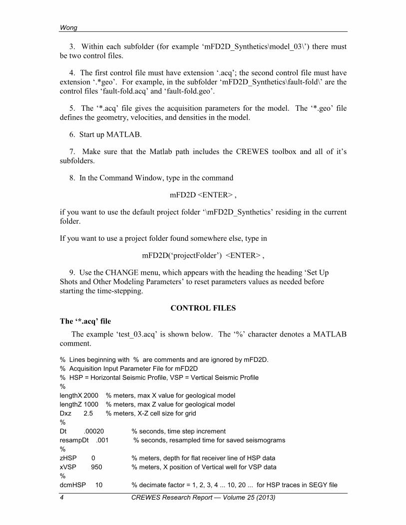
3. Within each subfolder (for example ‘mFD2D_Synthetics\model_03\’) there must be two control files.

4. The first control file must have extension ‘.acq’; the second control file must have extension ‘.*geo’. For example, in the subfolder ‘mFD2D_Synthetics\fault-fold\’ are the control files ‘fault-fold.acq’ and ‘fault-fold.geo’.

5. The ‘*.acq’ file gives the acquisition parameters for the model. The ‘*.geo’ file defines the geometry, velocities, and densities in the model.

6. Start up MATLAB.

7. Make sure that the Matlab path includes the CREWES toolbox and all of it’s subfolders.

8. In the Command Window, type in the command

mFD2D <ENTER> ,

if you want to use the default project folder ‘\mFD2D_Synthetics’ residing in the current folder.

If you want to use a project folder found somewhere else, type in

mFD2D(‘projectFolder’) <ENTER> ,

9. Use the CHANGE menu, which appears with the heading the heading ‘Set Up Shots and Other Modeling Parameters’ to reset parameters values as needed before starting the time-stepping.

CONTROL FILES The ‘*.acq’ file

The example ‘test_03.acq’ is shown below. The ‘%’ character denotes a MATLAB comment.

% Lines beginning with % are comments and are ignored by mFD2D. % Acquisition Input Parameter File for mFD2D % HSP = Horizontal Seismic Profile, VSP = Vertical Seismic Profile % lengthX 2000 % meters, max X value for geological model lengthZ 1000 % meters, max Z value for geological model Dxz 2.5 % meters, X-Z cell size for grid % Dt .00020 % seconds, time step increment resampDt .001 % seconds, resampled time for saved seismograms % zHSP 0 % meters, depth for flat receiver line of HSP data xVSP 950 % meters, X position of Vertical well for VSP data % dcmHSP 10 % decimate factor = 1, 2, 3, 4 ... 10, 20 ... for HSP traces in SEGY file



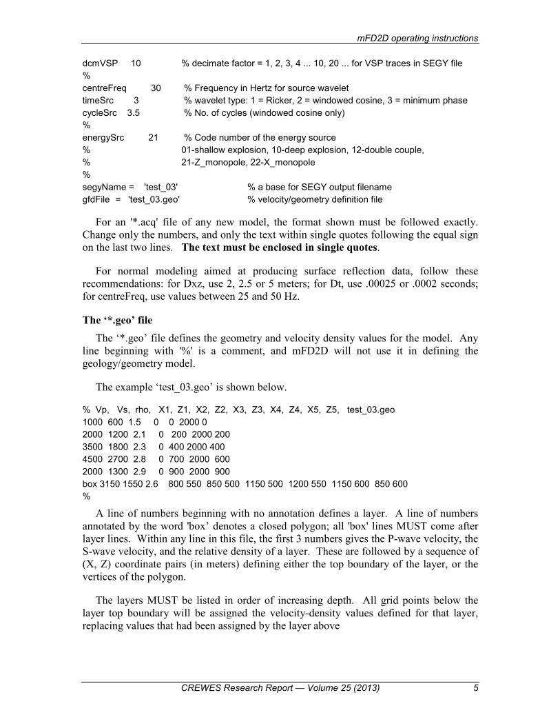
dcmVSP 10 % decimate factor = 1, 2, 3, 4 ... 10, 20 ... for VSP traces in SEGY file % centreFreq 30 % Frequency in Hertz for source wavelet timeSrc 3 % wavelet type: 1 = Ricker, 2 = windowed cosine, 3 = minimum phase cycleSrc 3.5 % No. of cycles (windowed cosine only) % energySrc 21 % Code number of the energy source % 01-shallow explosion, 10-deep explosion, 12-double couple, % 21-Z_monopole, 22-X_monopole % segyName = 'test_03' % a base for SEGY output filename gfdFile = 'test_03.geo' % velocity/geometry definition file

For an '*.acq' file of any new model, the format shown must be followed exactly. Change only the numbers, and only the text within single quotes following the equal sign on the last two lines. The text must be enclosed in single quotes.

For normal modeling aimed at producing surface reflection data, follow these recommendations: for Dxz, use 2, 2.5 or 5 meters; for Dt, use .00025 or .0002 seconds; for centreFreq, use values between 25 and 50 Hz.

The ‘*.geo’ file The ‘*.geo’ file defines the geometry and velocity density values for the model. Any

line beginning with '%' is a comment, and mFD2D will not use it in defining the geology/geometry model.

The example ‘test_03.geo’ is shown below.

% Vp, Vs, rho, X1, Z1, X2, Z2, X3, Z3, X4, Z4, X5, Z5, test_03.geo 1000 600 1.5 0 0 2000 0 2000 1200 2.1 0 200 2000 200 3500 1800 2.3 0 400 2000 400 4500 2700 2.8 0 700 2000 600 2000 1300 2.9 0 900 2000 900 box 3150 1550 2.6 800 550 850 500 1150 500 1200 550 1150 600 850 600 %

A line of numbers beginning with no annotation defines a layer. A line of numbers annotated by the word 'box’ denotes a closed polygon; all 'box' lines MUST come after layer lines. Within any line in this file, the first 3 numbers gives the P-wave velocity, the S-wave velocity, and the relative density of a layer. These are followed by a sequence of (X, Z) coordinate pairs (in meters) defining either the top boundary of the layer, or the vertices of the polygon.

The layers MUST be listed in order of increasing depth. All grid points below the layer top boundary will be assigned the velocity-density values defined for that layer, replacing values that had been assigned by the layer above

Wong


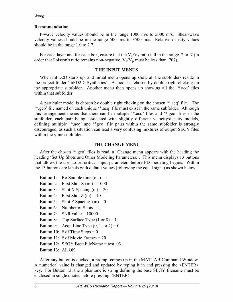
Recommendation P-wave velocity values should be in the range 1000 m/s to 5000 m/s. Shear-wave

velocity values should be in the range 500 m/s to 3500 m/s. Relative density values should be in the range 1.0 to 2.7.

For each layer and for each box, ensure that the Vs/Vp ratio fall in the range .2 to .7 (in order that Poisson's ratio remains non-negative, Vs/Vp must be less than .707).

THE INPUT MENUS When mFD2D starts up, and initial menu opens up show all the subfolders reside in

the project folder ‘mFD2D_Synthetics’. A model is chosen by double right-clicking on the appropriate subfolder. Another menu then opens up showing all the ‘*.acq’ files within that subfolder.

A particular model is chosen by double right clicking on the chosen ‘*.acq’ file. The ‘*.geo’ file named on each unique ‘*.acq’ file must exist in the same subfolder. Although this arrangement means that there can be multiple ‘*.acq’ files and ‘*.geo’ files in the subfolder, each pair being associated with slightly different velocity/density models, defining multiple ‘*.acq’ and ‘*geo’ file pairs within the same subfolder is strongly discouraged, as such a situation can lead a very confusing mixtures of output SEGY files within the same subfolder.

THE CHANGE MENU After the chosen ‘*.geo’ files is read, a Change menu appears with the heading the

heading ‘Set Up Shots and Other Modeling Parameters.’. This menu displays 13 buttons that allows the user to set critical input parameters before FD modeling begins. Within the 13 buttons are labels with default values (following the equal signs) as shown below.

Button 1: Re-Sample time (ms) = 1 Button 2: First Shot X (m ) = 1000 Button 3: Shot X Spacing (m) = 20 Button 4: First Shot Z (m) = 10 Button 5: Shot Z Spacing (m) = 0 Button 6: Number of Shots = 1 Button 7: SNR value = 10000 Button 8: Top Surface Type (1 or 8) = 1 Button 9: Acqn Line Type (0, 1, or 2) = 0 Button 10: # of Time Steps = 0 Button 11: # of Movie Frames = 20 Button 12: SEGY Base FileName = test_03 Button 13: All OK

After any button is clicked, a prompt comes up in the MATLAB Command Window. A numerical value is changed and updated by typing it in and pressing the <ENTER> key. For Button 13, the alphanumeric string defining the base SEGY filename must be enclosed in single quotes before pressing <ENTER>.



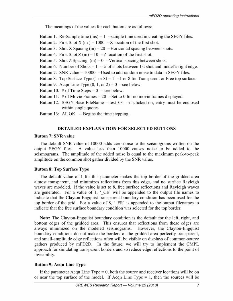
The meanings of the values for each button are as follows:

Button 1: Re-Sample time (ms) = 1 --sample time used in creating the SEGY files. Button 2: First Shot X (m ) = 1000 --X location of the first shot. Button 3: Shot X Spacing (m) = 20 --Horizontal spacing between shots. Button 4: First Shot Z (m) = 10 --Z location of the first shot. Button 5: Shot Z Spacing (m) = 0 --Vertical spacing between shots. Button 6: Number of Shots = 1 -- # of shots between 1st shot and model’s right edge. Button 7: SNR value = 10000 --Used to add random noise to data in SEGY files. Button 8: Top Surface Type (1 or 8) = 1 --1 or 8 for Transparent or Free top surface. Button 9: Acqn Line Type (0, 1, or 2) = 0 --see below. Button 10: # of Time Steps = 0 -- see below. Button 11: # of Movie Frames = 20 --Set to 0 for no movie frames displayed. Button 12: SEGY Base FileName = test_03 --if clicked on, entry must be enclosed

within single quotes Button 13: All OK -- Begins the time stepping.

DETAILED EXPLANATION FOR SELECTED BUTTONS Button 7: SNR value

The default SNR value of 10000 adds zero noise to the seismograms written on the output SEGY files. A value less than 10000 causes noise to be added to the seismograms. The amplitude of the added noise is equal to the maximum peak-to-peak amplitude on the common shot gather divided by the SNR value.

Button 8: Top Surface Type The default value of 1 for this parameter makes the top border of the gridded area

almost transparent, and minimizes reflections from this edge, and no surface Rayleigh waves are modeled. If the value is set to 8, free surface reflections and Rayleigh waves are generated. For a value of 1, ‘_CE’ will be appended to the output file names to indicate that the Clayton-Engquist transparent boundary condition has been used for the top border of the grid. For a value of 8, ‘_FR’ is appended to the output filenames to indicate that the free surface boundary condition was selected for the top border.

Note: The Clayton-Engquist boundary condition is the default for the left, right, and bottom edges of the gridded area. This ensures that reflections from these edges are always minimized on the modeled seismograms. However, the Clayton-Engquist boundary conditions do not make the borders of the gridded area perfectly transparent, and small-amplitude edge reflections often will be visible on displays of common-source gathers produced by mFD2D. In the future, we will try to implement the CMPL approach for simulating transparent borders and so reduce edge reflections to the point of invisibility.

Button 9: Acqn Line Type If the parameter Acqn Line Type = 0, both the source and receiver locations will be on

or near the top surface of the model. If Acqn Line Type = 1, then the sources will be

Wong


along the top surface, while the receivers will be located on the first layer boundary below the top surface. If Acqn Line Type = 2, both sources and receivers will be located on the first boundary beneath the top surface. Setting Acqn Line Type to a value of 2 can be used to generate data that simulates reflections along a 2D line on a surface with topography. See Appendix A for an example.

Button 10: # of Time Steps The number of time steps must be set large enough to cover the desired time window

Tmax for the final seismograms. For example, if Tmax is 0.800 seconds, and the time step Dt is .0002 seconds, then the number of time steps must be equal to 4000.

If # of Time Steps is set to zero, then no time-stepping will occur. Zero time steps enables the user to see in graphical form the source wavelet, the force pattern for the source, the geometry of the acquisition lines, and the velocity/density structure of the model before time-stepping occurs. They should be checked to see if all the control parameters are what the user expects them to be before time-stepping is allowed to proceed, since the full finite-difference modeling for even a single shot gather can take many minutes.

If the parameter values in the menu are satisfactory, clicking on the All OK button will initiated the time-stepping calculations. When the time-stepping is completed, four files will be written, one each for the x- and z-component seismograms for horizontal seismic profile (HSP) and the vertical seismic profile (VSP). The seismograms are located at received positions defined by the relevant parameters in the Parameters menu, and by the decimation factors dcmHSP and dcmVSP in the ‘*.acq’ text file.

It is strongly recommended that a single shot gather, with the shot placed near the centre of the top surface and with the requisite number of time steps, be generated to gauge total execution BEFORE modeling a full 2D lines with many shot points..

Button 11: # of Movie Frames This number gives the number of propagation snapshots to be shown as the time

stepping proceeds. If zero is entered, no snapshots will be displayed.

Button 12: SEGY Base FileName This alphanumeric string is the base name of the four SEGY files that will be written

after the total number of time steps has been reached. The user can change this after clicking on this button. When entering a new name, it must be enclosed by single quotes.

Button 13: # All OK When the parameters indicated next to all the buttons are satisfactory, clicking on

ALL OK begins the time-stepping.



STABILITY CONDITIONS

Let 𝑉𝑚𝑖𝑛 be the smallest S-wave velocity in the model. Let 𝑓𝑑 be the value for the dominant frequency in the source wavelet. Define

𝜆𝑚𝑖𝑛= 𝑉𝑚𝑖𝑛/𝑓𝑑 . (1) According to the theory for finite difference time-step of elastic wave propagation in

two dimensions, numerical results require that two conditions be met:

𝐷𝑥𝑧 < 𝜆𝑚𝑖𝑛/10 , (2)

𝐷𝑡 < √2 ∙ 𝐷𝑥𝑧/𝑉𝑚𝑎𝑥 , (3)

where 𝐷𝑥𝑧 is the spatial sampling interval, 𝐷𝑡 is the time-stepping interval and 𝑉𝑚𝑎𝑥 is the largest P-wave velocity in the model. We take 𝑓𝑑 to be equal to source wavelet CentreFreq parameter as defined in the ‘*.acq’ file.

The limitation on the grid size 𝐷𝑥𝑧 is based on an error criterion regarding how closely numerical spatial derivatives must approximate the analytic derivatives. The limitation on the time-step 𝐷𝑡 is determined by the Courant number for stable 2D finite-difference numerical modeling (Kosloff and Baysal, 1982; Carcione, 1995). These limits on 𝐷𝑥𝑧 and 𝐷𝑡 theoretically ensure stability of the finite difference time-stepping technique. If 𝐷𝑥𝑧 and 𝐷𝑡 are grossly out of agreement with Equations 2 and 3, grid dispersion artifacts, characterized by late-arriving high-frequency coda immediately following each ‘valid’ event, will appear in the final seismograms. In the worst case scenario, stabilities will set in, and the numerical technique may fail catastrophically.

The implementation of the numerical finite-difference scheme used within mFD2D.m requires more stringent limits on the values of 𝐷𝑥𝑧 and 𝐷𝑡. Values for 𝐷𝑥𝑧 and 𝐷𝑡 typically found in the ‘*.acq’ files are much less than those indicated by Equations 1 to 3. For heterogeneous velocity models in which zones of very low velocity co-exist with zones of very high velocities, even smaller values are necessary, but it may be difficult to find values that avoid the onset of instabilities at the later time-steps. It must be emphasized that, for a given model size, very small values of 𝐷𝑥𝑧 will lead to excessive memory requirements, and small values of 𝐷𝑡 would result in a large number of time steps in order to yield seismograms with the required maximum trace length.

If the low-velocity zones are limited in size and number (for example, a relatively thin overburden, or a thin coal bed imbedded in high-velocity sandstone layer), useful results still may be obtained with values of 𝐷𝑥𝑧 and 𝐷𝑡 not in strict conformance with conditions (2) and (3) for all zones, as long as they are met for the bulk of the model. In cases with a low-velocity overburden, reflection events from deeper high velocity layers may still be true, even though the direct arrivals through the overburden and Rayleigh wave (ground roll) events may show dispersion and ringing. The user can experiment with the values of 𝐷𝑥𝑧 and 𝐷𝑡 for models with low-velocity overburden to see whether or not, in his opinion, the modeled common-source gathers have a satisfactory appearance.

Two ways of avoiding or minimizing the visible dispersions associated with arrivals through low-velocity overburdens are:

Wong


• use S-wave velocities greater than 1500 m/s, or

• model with the top surface designated to be transparent and not free, so that no Rayleigh waves are generated.

Oftentimes, the surface wave and direct arrivals are of little interest. In such cases, they can be completely eliminated to reveal subsurface reflections more clearly by following this procedure:

(a) Create common-source gathers for a model with only near-surface, low-velocity structure, and save the resulting seismograms in a named SEGY file.

(b) Create the same common-source gathers after adding subsurface structure to the model in (a), and save the seismograms in a differently named SEGY file.

(c) In processing, subtract the seismic data in file (a) from the seismic data in file (b). AGC displays of the difference traces will show reflection arrivals without interference caused by surface-wave and direct arrivals.

Warning: During the late stages of time-stepping, a movie frame may begin to display black zones. This is a clear indication that instabilities are building up. The likeliest cause is that the grid size 𝐷𝑥𝑧 is too small to adequately satisfy Equations 1 to 3. Upon completion of the time-stepping in such a case, the seismograms written into the SEGY files may still have a ‘normal’ appearance, but more likely the files will contain zero-value traces.

ACKNOWLEDGEMENTS This research has been supported by the Natural Sciences and Engineering Research

Council of Canada (NSERC) and the industrial sponsors of CREWES.

REFERENCES Clayton, R., and Engquist, B., 1977. Absorbing boundary conditions for acoustic and elastic wave

equations: Bulletin, Seismological Society of America, 67, 1529–1540. Manning, P.M., 2007. Techniques to enhance the accuracy and efficiency of finite-difference modelling for

the propagation of elastic waves, Ph.D. dissertation, University of Calgary. Kosloff, D., and Baysal, E., 1982. Forward modeling by a Fourier method: Geophysics, 47, 1402-1412. Virieux, J., 1986. P-SV wave propagation in heterogeneous media: velocity-stress finite-difference

method: Geophysics, 51, 889-901. Wong, J. and Manning, P.M., 2012. Elastic wave 2D modeling of seismic surveys: CREWES Research

Report, 24, 80.1-80.18.



APPENDIX A: MODELING TOPOGRAPHIC EFFECTS Button 9: Acqn Line Type

If the parameter Acqn Line Type is set to 0, both the source and receiver locations will be on or near the top surface of the model. If Acqn Line Type is set to 1, then the sources will be along the top surface, while the receivers will be located on the first layer boundary below the top surface. If Acqn Line Type set to 2, then sources and receivers are both located on the first layer boundary below the top surface. If this boundary is defined with topography, and if the velocities and densities of the top and second layers are given identical values, the modeling will simulate reflection seismograms for a survey carried out along a line with topography.

Reflections will occur from the top surface, but they can be eliminated by running the modeling twice. The first time, define velocity and density values for all layers to be homogeneous and equal to that of the first and second layers. The second time, include values for velocity and density to define the structure below the second layer. Make sure that the SEGY Base Filenames for these two cases are different. The difference between the seismograms in these two files will show only reflections from the subsurface structure but obtained on a surface with topography.

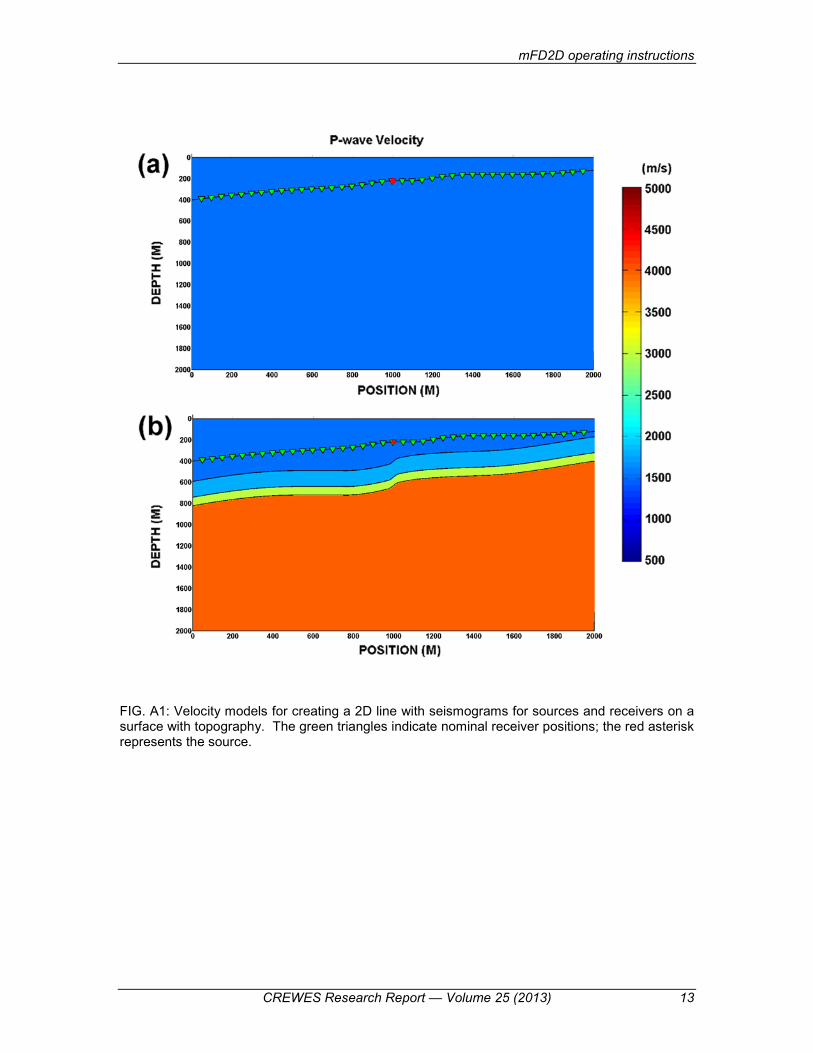
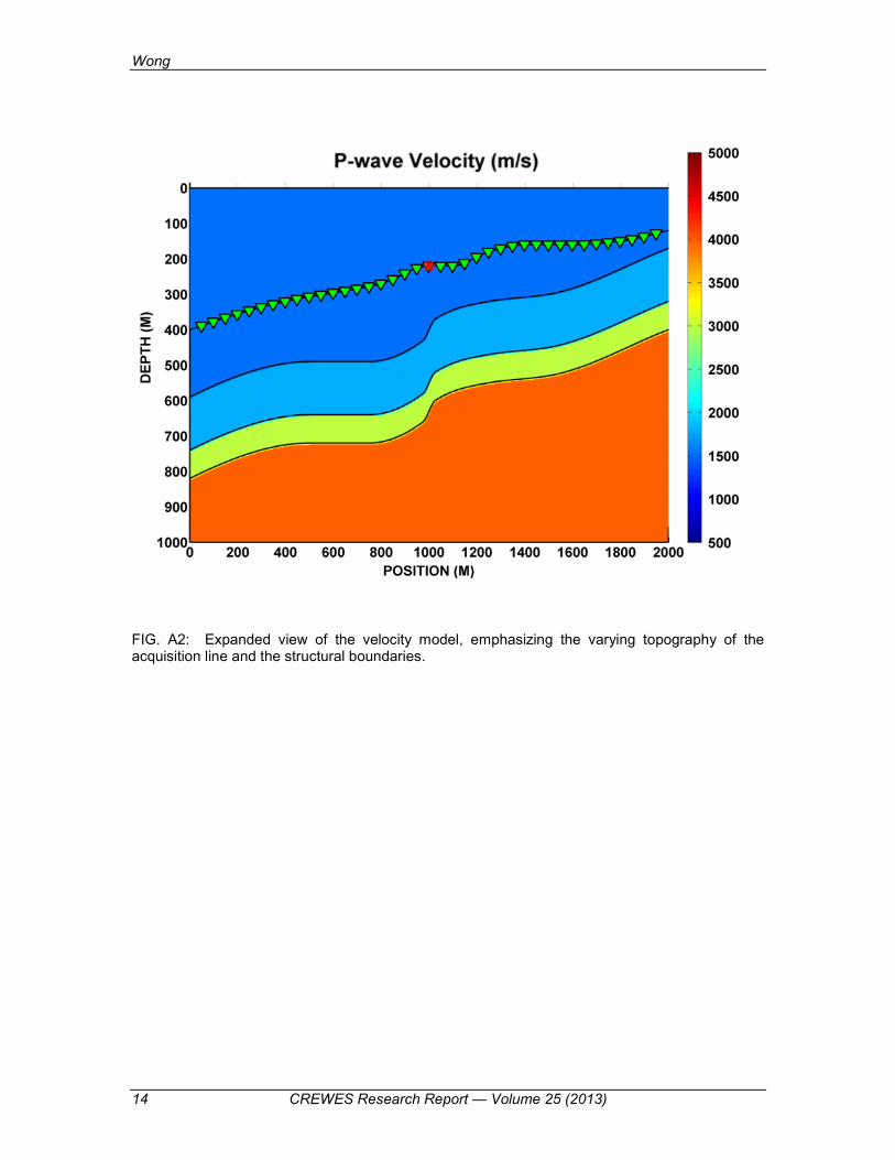
Figures A1 to A4 demonstrates how to create a dataset that includes topographic effects. Figures A1(a) shows a homogeneous initial model with an acquisition line along a non-flat boundary at some depth below the top surface of the grid. Figures A1(b) shows the same model but with structure beneath the acquisition line. Figure A2 is an expanded view of Figure A1(b) emphasizing the topography along the acquisition line.

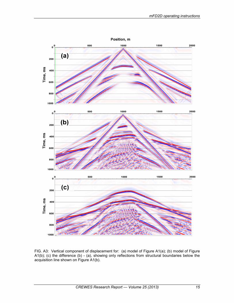
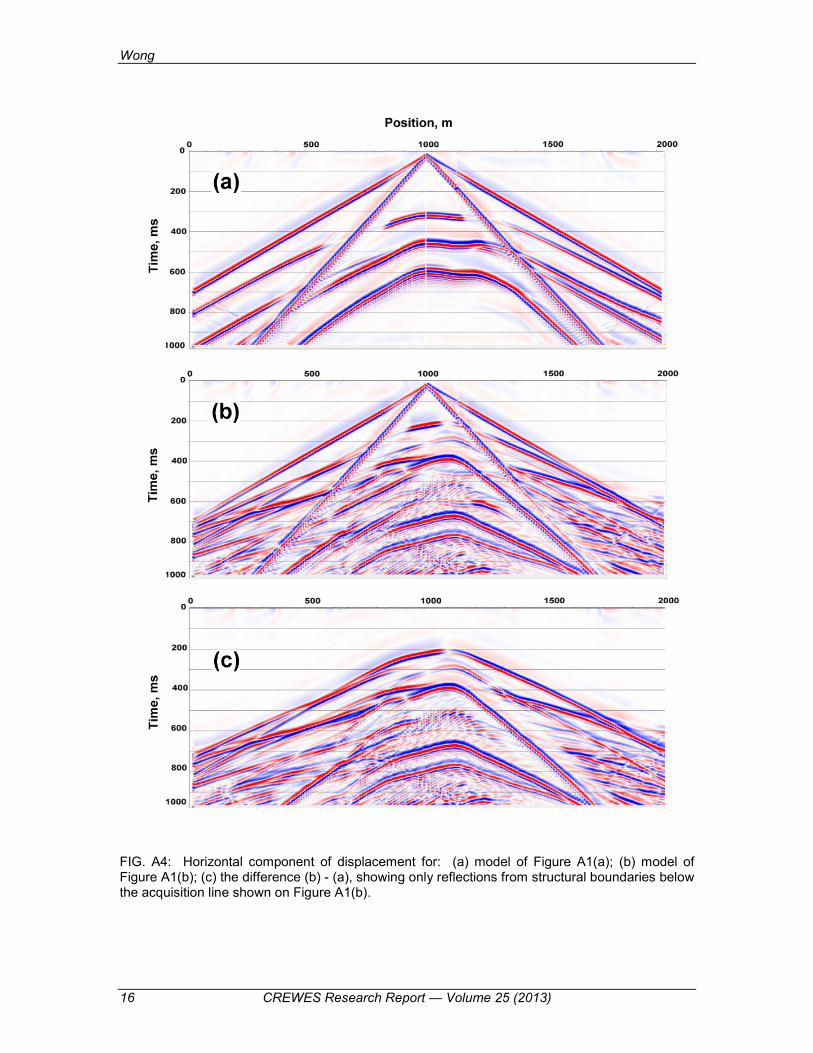
On Figure A3, we display the vertical component seismograms resulting from the mFD2D modeling. Figure A3(a) are seismograms from the homogeneous model, while Figure A3(b) are the seismograms from the structured model. The difference between the two sets of seismograms is shown on Figure A3(c). The difference seismograms exclude edge reflections, surface waves, and direct arrivals, and isolate the deep reflections. The horizontal-component seismograms for the homogeneous and structured models are shown on Figure A4(a) and A4(b); their difference is shown on Figure A4(c).

The input control files for the above example are found in the subfolder ‘c:\mFD2D_Synthetics\Topographic Line’. The ‘topo_1.acq’ file for the homogeneous model is the following:

% Lines beginning with % are comments and are ignored by mFD2D. % Acquisition Input Parameter File for mFD2D % HSP = Horizontal Seismic Profile, VSP = Vertical Seismic Profile % lengthX 2000 % meters, max X value for geological model lengthZ 2000 % meters, max Z value for geological model Dxz 2.0 % meters, X-Z cell size for grid % Dt .00025 % seconds, time step increment resampDt .001 % seconds, resampled time for saved seismograms % zHSP 0 % meters, depth for flat receiver line of HSP data

Wong


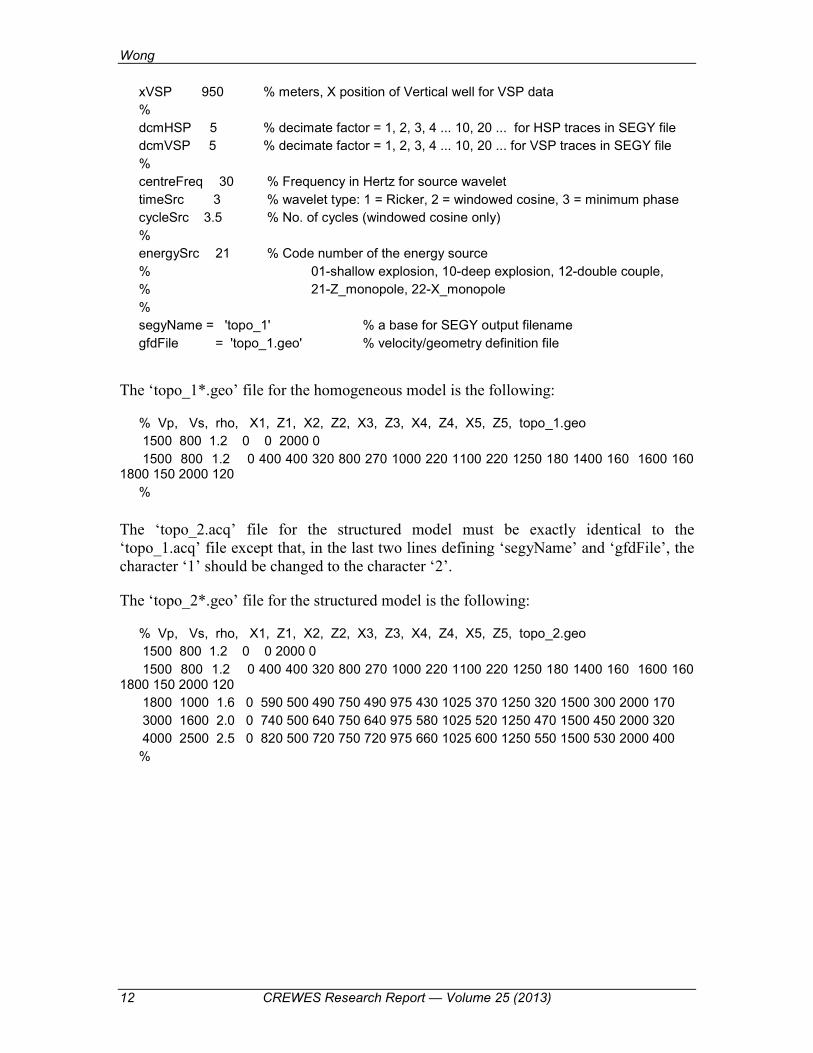
xVSP 950 % meters, X position of Vertical well for VSP data % dcmHSP 5 % decimate factor = 1, 2, 3, 4 ... 10, 20 ... for HSP traces in SEGY file dcmVSP 5 % decimate factor = 1, 2, 3, 4 ... 10, 20 ... for VSP traces in SEGY file % centreFreq 30 % Frequency in Hertz for source wavelet timeSrc 3 % wavelet type: 1 = Ricker, 2 = windowed cosine, 3 = minimum phase cycleSrc 3.5 % No. of cycles (windowed cosine only) % energySrc 21 % Code number of the energy source % 01-shallow explosion, 10-deep explosion, 12-double couple, % 21-Z_monopole, 22-X_monopole % segyName = 'topo_1' % a base for SEGY output filename gfdFile = 'topo_1.geo' % velocity/geometry definition file

The ‘topo_1*.geo’ file for the homogeneous model is the following:

% Vp, Vs, rho, X1, Z1, X2, Z2, X3, Z3, X4, Z4, X5, Z5, topo_1.geo 1500 800 1.2 0 0 2000 0 1500 800 1.2 0 400 400 320 800 270 1000 220 1100 220 1250 180 1400 160 1600 160

1800 150 2000 120 %

The ‘topo_2.acq’ file for the structured model must be exactly identical to the ‘topo_1.acq’ file except that, in the last two lines defining ‘segyName’ and ‘gfdFile’, the character ‘1’ should be changed to the character ‘2’.

The ‘topo_2*.geo’ file for the structured model is the following:

% Vp, Vs, rho, X1, Z1, X2, Z2, X3, Z3, X4, Z4, X5, Z5, topo_2.geo 1500 800 1.2 0 0 2000 0 1500 800 1.2 0 400 400 320 800 270 1000 220 1100 220 1250 180 1400 160 1600 160

1800 150 2000 120 1800 1000 1.6 0 590 500 490 750 490 975 430 1025 370 1250 320 1500 300 2000 170 3000 1600 2.0 0 740 500 640 750 640 975 580 1025 520 1250 470 1500 450 2000 320 4000 2500 2.5 0 820 500 720 750 720 975 660 1025 600 1250 550 1500 530 2000 400 %



FIG. A1: Velocity models for creating a 2D line with seismograms for sources and receivers on a surface with topography. The green triangles indicate nominal receiver positions; the red asterisk represents the source.

Wong


FIG. A2: Expanded view of the velocity model, emphasizing the varying topography of the acquisition line and the structural boundaries.



FIG. A3: Vertical component of displacement for: (a) model of Figure A1(a); (b) model of Figure A1(b); (c) the difference (b) - (a), showing only reflections from structural boundaries below the acquisition line shown on Figure A1(b).

Wong


FIG. A4: Horizontal component of displacement for: (a) model of Figure A1(a); (b) model of Figure A1(b); (c) the difference (b) - (a), showing only reflections from structural boundaries below the acquisition line shown on Figure A1(b).