Operation Manual HYPROP - METERlibrary.metergroup.com/Manuals/UMS/Hyprop_Manual.pdf · Operation Manual HYPROP ... In case a balance does not show, check ... Short cuts to key functions

Operation Manual

HYPROPThis manual is also available in German:www.ums-muc.de/static/Bedienungsanleitung_HYPROP.pdf

At a glance – how it works

Evaporation

Soil sample

Sampling ring

Balance

Tensio Top

Tensio Bottom

to USB interface

Pressure sensors

Sensor unit

HYPROP® is a fully automated measuring and evaluation system to determine the hydraulic properties of soil samples. HYPROP measures the water tension at two levels of a sample using two tensio shafts. If the conductivity of the sample is poor the soil in the upper horizons dries out whereas the lower horizons are still humid. So the upper tensio shaft measures much drier tensions than the lower one which is still humid. If the conductivity is good water is evaporated out of the whole sample and both tensions are almost identical. The water content for the pF/WC curve is calculated based on the weight loss of the sample.

This measuring concept is based on Schindler’s method. Please find further information in the chapter “Theory”.

Legend

water electronics soil

water vapor ceramic all other parts cross section of a part

Parts of the deviceand scope of delivery

sample ring

sensor unit

O-ring (red) for sealing the tensio shafts

to the pressure sensor

ceramic

shaft

silicone gasket

tensio shafts

O-ring (black) for dirt protection

balance

Note This manual does not describe the evaluation of the measuring data using the HYPROP-FIT software. For this please find another manual: http://www.ums-muc.de/static/Manual_HYPROP-FIT.pdf

Additional parts in the scope of delivery

sens

or u

nit

O-r

ing

s

tens

io s

hafts

50 m

m a

nd 2

5 m

mH

YPR

OP

co

nne

ctin

g c

ab

le

pla

stic

ca

ps

silic

one

ga

ske

t and

no

nwo

ven

clo

ths

tens

ioLi

nk®

T-p

iec

e

refil

ling

atta

chm

ent

fo

r se

nso

r uni

tsa

tura

tion

pla

te

5 | Scope of delivery

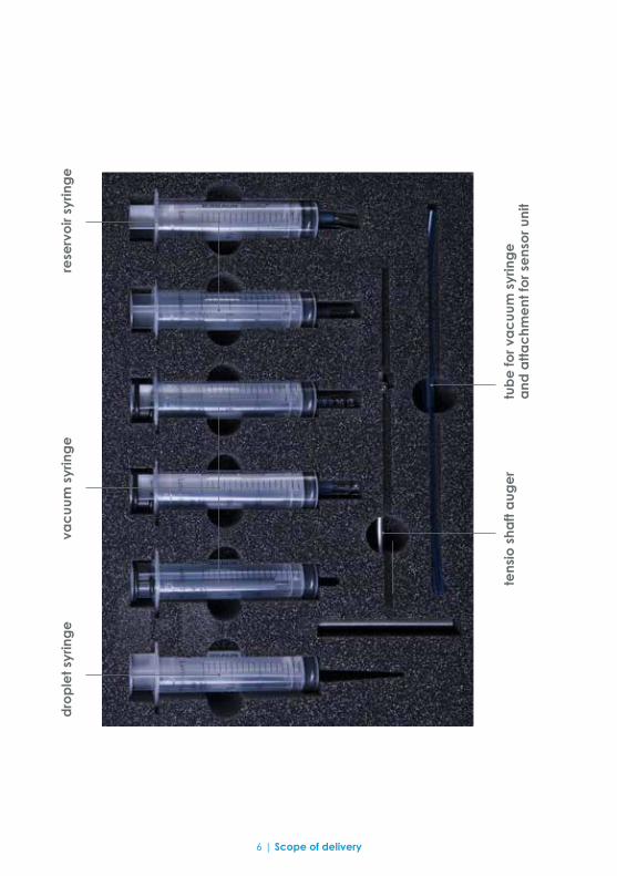
dro

ple

t syr

ing

e

tens

io s

haft

aug

er

tub

e fo

r va

cuu

m s

yrin

ge

and

atta

chm

ent

for s

ens

or u

nit

vac

uum

syr

ing

ere

serv

oir

syrin

ge


aug

er g

uid

e

sam

ple

ring

250

ml

with

pla

stic

ca

ps

de

ioni

zed

wa

ter

po

we

r de

vic

e

HY

PRO

P U

SB a

da

pte

r


8 | Content

Contents At a glance – how it works ................................................................................... 2Parts of the device and scope of delivery .......................................................... 3 Important information ......................................................................................... 10 Safety instructions ............................................................................................10 Intended use ....................................................................................................10 Warranty ...........................................................................................................10HYPROP-VIEW software functions ....................................................................... 11 Key functions ....................................................................................................11 User support .....................................................................................................11 Show devices ...................................................................................................12 Device tree ......................................................................................................13Initial operation .................................................................................................... 16 Software installation: HYPROP-VIEW and HYPROP-FIT .................................16 Hardware configuration ..................................................................................17 How to use the tube connections . ................................................................18General measuring procedure .......................................................................... 19Preparing the measurement .............................................................................. 20 Saturating the soil sample ..............................................................................20 Filing the device ..............................................................................................22 using the Refill Unit (accessories) ..........................................................23 using syringes ...........................................................................................28 Implementing the tensio shafts in the sensor unit ........................................41 Attaching the dirt protection .........................................................................44 Function check ................................................................................................45 Assembling the sensor unit and the soil sample ..........................................47 Connecting the sensor unit and the balance .............................................49 Preparing the balance ...................................................................................51 Adjusting ............................................................................................................53 Default settings .................................................................................................55Measuring ............................................................................................................ 56 Multi balance mode (one balance per sensor unit) ..................................56 Single balance mode (one balance for more sensor units) ......................57Optimal measuring curve ................................................................................... 59 Notes on suboptimal measuring curves .......................................................61Finishing a measurement .................................................................................... 62

Determining the dry weight ................................................................................ 65 Weighing the dry mass ....................................................................................66Evaluating the measurement ............................................................................. 67Trouble shooting .................................................................................................. 68Cleaning and maintenance ............................................................................... 69 Cleaning the sensor unit .................................................................................69 Changing the O-rings in the sensor unit .......................................................70 Storage .............................................................................................................71Additional accessories ....................................................................................... 72Theory ................................................................................................................... 74 Preliminary note ...............................................................................................74 Measuring method ..........................................................................................75 Explanation of terms ........................................................................................76 Generating data points ..................................................................................78 Additional notes ..............................................................................................80Addendum ........................................................................................................... 81 Typical measuring curves ...............................................................................81 Standard pF curves .........................................................................................88 Procedure of sampling for WP4 measurements after a HYPROP measurement .......................................................................89 Units for soil water and matrix potentials ......................................................89Facts and figures ................................................................................................. 91 Technical data ................................................................................................91Literature cited ..................................................................................................... 92

9 | Content

Important information

10 | Important information

Electrical installations must meet the safety and EMC requirements of the country in which the system is used. Damages caused by the user are not covered by the warranty. HYPROP is a device to measure soil tensions as well as soil water pressures and temperatures and is only intended for this parti-cular use. Please keep the following notes in mind:

Note

Please do not touch the ceramic of the tensio shafts with bare fingers. Grease or soap reduces the hydrophilic characteristics of the ceramic.

Note

Do not stick sharp objects into the holes of the sensor unit. You may damage the pressure sensor.

Intended use

Safety instructions

Warranty

HYPROP® is a measuring system that is intended to be used for measuring the water retention function and the hydraulic conductivity as a function of the water tension or the water content of soil samples.

UMS offers a warranty for material and production defects for this device in accordance with the locally applicable legal provisions, but for a minimum of 12 months. The warranty does not cover damage caused by misuse, inex-pert servicing or circumstances beyond our control. The warranty includes replacement or repair and packing but excludes shipping expenses. Please contact UMS or our representative before returning equipment. Place of ful-fillment is Gmunder Str. 37, Munich, Germany.

Software functions

The key functions are:• displaying the connected devices,• displaying the measurement data• filling assistant• measurement configuration wizard

The wizard is explained in the respective chapter.

User support

Key functions

Example of user support: Help Function

Note After starting the software the user support leads you through all software functions. If you are an experienced user you may not like to use the wizard of the measuring configuration and enter the data directly instead. This is possible too.

When you start the software and the help function is activated notes of the next step are displayed, e.g. here you are asked to click on the “Show device” icon.

11 | Software functions

Show connected devices

Click on an icon in the upper screen bar e.g. “Measurement”.

Click on the icon “Show devices”.

In case a balance does not show, check if the balance is switched on.

Follow the wizard.

When all steps are done, click on “Apply” if you want to enter the configuration.If you click on “Cancel” you return to the initial page, where you have opened the wizard.

Data you have entered are set in the program.

All connected balances and sensor units are displayed.

Example of user support: Wizard


The device tree (example)

Sensor unit “soil lab 18” is connected to the computer via a HYPROP balance.

Sensor unit “soil lab 15” is connected to the computer via the USB adapter.

A Kern balance is connected to the computer via a RS232 interface.

Sensor unit “soil lab 17” is connected to the computer via a HYPROP USB Cable.


Main window with manager

Mode (one or more balances)

Connected devices

One measurement file per soil sample is generated

Data to be typed in by the user

Device ID (click right mouse button to change)

Short cuts to key functions Unit Link to the HYPROP-FIT

softwareNext step

Switches to displaying the measurement values when a mea-surement is running

Default folder for measurement files

Interrupt, stop or start all measurements


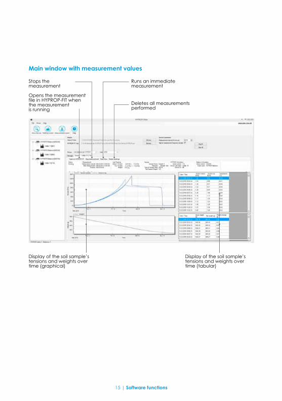
Main window with measurement values

Stops the measurement

Runs an immediate measurement

Display of the soil sample’s tensions and weights over time (graphical)

Display of the soil sample’s tensions and weights over time (tabular)

Opens the measurement file in HYPROP-FIT when the measurement is running

Deletes all measurements performed


Initial operation

Put the CD with the HYPROP software into the computer. If you do not have a CD download the software using the link www.ums-muc.de/static/HYPROP.zip. Double click on Setup.exeFollow the wizard.

Connect the HYPROP balance to the USB port.

Start the HYPROP software.

The wizard leads you through the installation.

The balance connects automatically to the computer.

Your HYPROP is ready to measure.

Note For installing the HYPROP software you may need administrator rights.

Software installation: HYPROP-VIEW and HYPROP-FIT.

16 | Initial operation

Hardware configuration

Change device IDEach sensor unit needs its particular device ID otherwise a communication collision may occur.

Click on device with right mouse button.

Click on “apply”.

Choose “Chance Device ID”.

Choose an available ID from the pulldown menu.

Click on device with right mouse button.Choose “Rename”.

Click on “apply”.

Change device name (optional)


Note Cut the tube always rectangular otherwise the connection will be leaking.

To connect the tube to the fitting push the tube in as far as it will go.

To remove the tube press blue ring and pull.

How to use the tube connections


General measuring procedure

A measurement consists of the following steps:• soil sampling and preparation• saturating the soil sample• preparing the measuring system• setting up the sample in the measuring system and starting the measuring campaign• evaluating the measuring results with HYPROP-FIT.

In the following this manual will guide you through the measuring process step-by-step.

19 | General measuring procedure

Take the sample ring with soil out of the transport box and clean it. Prepare top and bottom side of the sample (e. g. with a saw blade).

Put a plastic cap upside down on the sample ring – on the side where the ring has the cutting edge. The cap works as a support. This makes sure that no soil gets lost even when loose sand is in the sample ring.

Preparing the measurement

Saturating the soil sample

20 | Preparing the measurement

Turn soil sample upside down and put it on a table. Remove cap on top, place nonwoven cloth on the soil and put the filling bowl on the sample ring.

Turn soil sample again upside down.

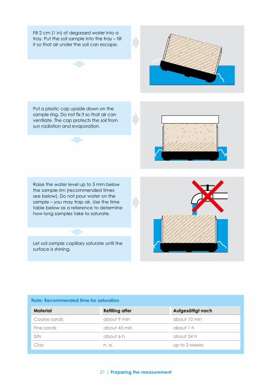
Note: Recommended time for saturation

Material Refilling after Aufgesättigt nach

Coarse sands about 9 min about 10 min

Fine sands about 45 min about 1 h

Silts about 6 h about 24 h

Clay n. a. up to 2 weeks

Raise the water level up to 5 mm below the sample rim (recommended times see below). Do not pour water on the sample – you may trap air. Use the time table below as a reference to determine how long samples take to saturate.

Fill 2 cm (1 in) of degassed water into a tray. Put the soil sample into the tray – tilt it so that air under the soil can escape.

Let soil sample capillary saturate until the surface is shining.

Put a plastic cap upside down on the sample ring. Do not fix it so that air can ventilate. The cap protects the soil from sun radiation and evaporation.


Filling the device

The tensio shafts “transduce” the matrix potentials (also called tensions) of the soil sample through their porous ceramic tip and the water filled shaft to the pressure sensors in the sensor unit. I.e. the tensio shafts provide via their pores a capillary contact between the water in the tensio shaft and the soil water.

To make sure the pressure is “transduced” precisely no air must be contained (dissolved or solved) in the water. That is why the tensio shafts and the sensor unit need to be degassed completely.

For degassing the water you can use two different methods:1. by means of the Refill Unit (accessory) makes all necessary

steps simple and is fast.2. by means of syringes (basic scope of delivery) takes some

more time and needs more manual work.

In the following either method is described in detail.


Degassing the device using the HYPROP Refill Unit

Hig

h p

erfo

rma

nce

va

cuu

m

pum

p e

nab

les

ge

nera

ting

a

va

cuu

m v

alu

e th

at i

s o

nly

8 hP

a (

0.8

kPa

)

Sco

pe

:

Va

cuu

m m

oun

t (in

clu

din

g

ma

nom

ete

r and

va

cuu

m

flask

, to

avo

id w

ate

r ent

ry

into

the

pum

p)

Ma

nom

ete

r

Bea

ker m

oun

t with

2

be

ake

rs. U

p to

10

b

ea

ker m

oun

ts c

an

b

e c

onn

ec

ted

in s

erie

s.En

d fi

tting

w

ith v

alv

e


Connect the devices of the Refill Unit as shown. Tubes and fittings that need to be connected are indicated by the same color.

Put the vacuum pump on the ground (lower temperature) to gain better vacuum values.

Connect the unit to a timer and the timer to the mains

Note We recommend to use a timer as this increases the pump life, reduces energy consumption and air bubbles that may be there are ripped off when the pump starts. The timer is not in the scope of delivery as the electrical requirements vary from country to country.

We also recommend with every degassing procedure to degas an additional bottle of deionized water. You will need the water when you fill the tensio shafts.

Note Do not touch the ceramic of the tensio shafts with bare fingers. Grease or soap reduces the hydrophilic characteristics of the ceramic.

The water in the tensio shaft evaporates to the ambient air. Therefore cover the tensio shaft tip with a silicone cap.


Fill holes of the sensor unit bubble free. For this use the droplet syringe.

Set up refilling attachment and fix it. Fill attachment with droplet syringe – ideally bubble free.

Filling the sensor unit

Note Do not stick the syringe tip into the holes of the sensor unit. You may damage the pressure sensor.


Timer starts the pump automatically and works in the rhythm set. The water in the tensio shafts is degassed after minimum 24 h running time.

Screw 1, 2, 3 or 4 tensio shafts into the adapters.

Put blind plugs on connections not used.

Close valve of the beaker unit.

Fill beaker(s) with deionized water.

Set timer according to a rhythm of e.g. 5 min “on” and 55 min “off”.

valve

Note If the manometer of the vacuum mount drops rapidly the system is leaking. Please check, fix leakage and restart degassing procedure. If you use another pump than the HYPROP pump, make sure that it is able to provide a vacuum value that is 8 hPa (0.8 kPa) below atmospheric air pressure. The power does not matter! Vacuum pumps that reach only a smaller vacuum value are not suitable.


Turn pump off. Open valve slowly and cautiously.

When the water in the tensio shafts and the sensor unit has been degassed you can continue to set up the HYPROP (see chapter “Implementing the tensio shafts into the sensor unit”).

Bringing the HYPROP Refill Unit back to ambient pressure

Note Never remove a tube in order to ventilate the system. The sudden pressure shock will damage the pressure sensors in the sensor unit.


If you have time put the tensio shafts in deionized water over night. Then the degassing takes less time. No water must enter the shaft from above, otherwise air will be locked in the pores.

Note

Do not touch the ceramic of the tensio shafts with bare fingers. Grease or soap reduces the hydrophilic characteristics of the ceramic.

The water in the tensio shaft evaporates to the ambient air. Therefore cover the tensio shaft tip with a silicone cap.

Degassing the device using syringes

1,5

cm


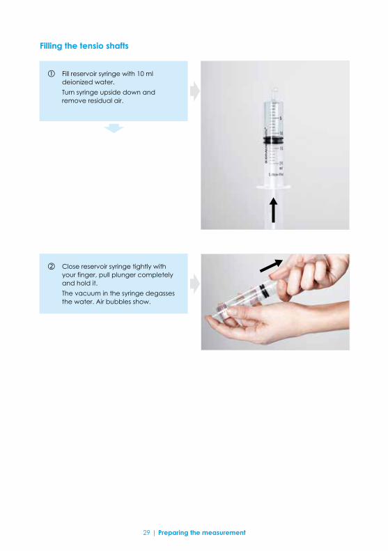
Fill reservoir syringe with 10 ml deionized water.

Turn syringe upside down and remove residual air.

Close reservoir syringe tightly with your finger, pull plunger completely and hold it.

The vacuum in the syringe degasses the water. Air bubbles show.

Filling the tensio shafts


Toss and turn reservoir syringe to “catch” air bubbles.


Turn syringe upside down and remove residual air.

Push tube piece onto the tip of the syringe.

Push plunger of the syringe until a menis-cus builds up on the tube piece.

Push the ceramic of the first tensio shaft into the tube piece.

Repeat step to until air bubbles do no show anymore.


Fill vacuum syringe with 5 ml deionized water. Turn syringe upside down and remove residual air.

Degas water in the vacuum syringe – analogous to degassing the reservoir syringe.

Push tube piece over the tip of the syringe.

Push plunger of the syringe until a meniscus builds up on the tube piece.


Connect the two syringes and the tensio shaft.

The two O-rings help seal the tubes against the tensio shaft shaft.

Pull out the plunger of the vacuum syringe …


… until the plunger stoppers snap in. The vacuum in the syringe removes the air from the tensio shaft.

Hold plunger and syringe, press in the plunger stoppers and let the plunger slowly move forward.

plunger stoppers plunger stoppers


Remove syringe, turn it upside down and remove residual air.

Push vacuum syringe bubble free onto the tensio shaft shaft again.

Degas water in the second tensio shaft.

For this repeat step to until air bubbles do not show anymore.


Fill holes of the sensor unit bubble free with deionized water. Use droplet syringe.

Filling the sensor unit

Note Do not stick the syringe tip into the holes of the sensor unit. You may damage the pressure sensor.

Set up refilling attachment and fix it. Fill attachment with droplet syringe – ideally bubble free.


Push blue tube piece onto the vacuum syringe and fill the tube.

Fill vacuum syringe with 15 to 20 ml deio-nized water. Degas water in the syringe as explained on the previous pages.

Connect blue tube onto to the fitting of the refilling attachment.

Pull out the plunger of the vacuum syringe until the plunger stoppers snap in.

The vacuum in the syringe removes the air from the sensor unit and its attachment. Air bubbles show.

Note Be extremely cautious! Do not let the plunger of the syringe shoot down as the pressure shock will damage the pressure sensor.


Let the air bubbles rise up into the tube by cautiously knocking and shifting the sensor unit.

Note In no case push the sensor unit on a hard surface! The impact will cause pressure shocks that damage the pressure sensors.


To relieve pressure hold plunger and syringe, press in the plunger stoppers and let the plunger slowly move forward.

Remove syringe from the tube, turn it upside down and remove residual air.

Repeat steps to until air bubbles do not show anymore.

Note Be extremely cautious! Do not let the plunger of the syringe shoot down as the pressure shock will damage the pressure sensor.


Push vacuum syringe filled with degassed water into the tube on the refilling attachment. Pull plunger until the plunger stoppers snap in. The pressure shown on the screen must reach a vacuum value equal to the atmospheric air pressure minus 20 hPa (2 kPa).

If this value can be reached the sensor unit is ready to measure after about 3 hours.

Note If the vacuum value does not reach a pressure equal to the atmospheric air pressure minus 20 hPa (2 kPa), then there is most likely:

• a dead volume in the syringe,• air in the tube • or a leakage in the system (e.g. between the sensor unit and the attachment)

After you have fixed the problem you need to degas the system again.


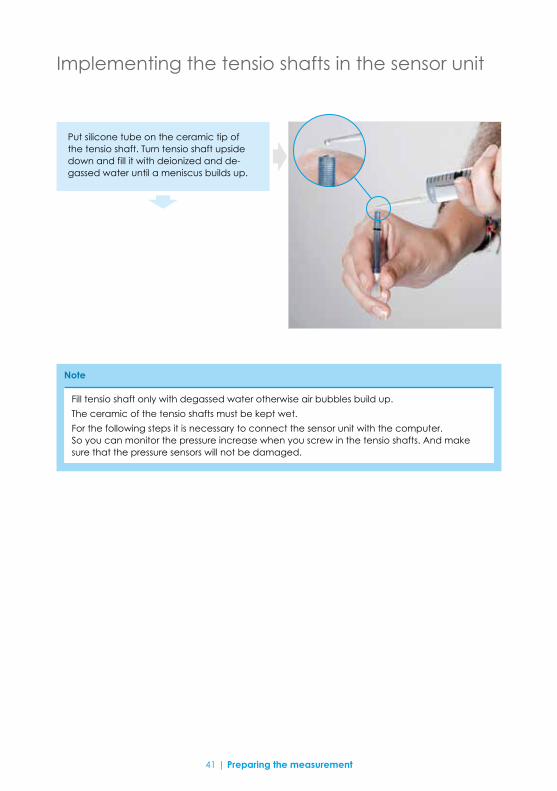
Put silicone tube on the ceramic tip of the tensio shaft. Turn tensio shaft upside down and fill it with deionized and de-gassed water until a meniscus builds up.

Implementing the tensio shafts in the sensor unit

Note Fill tensio shaft only with degassed water otherwise air bubbles build up.

The ceramic of the tensio shafts must be kept wet.

For the following steps it is necessary to connect the sensor unit with the computer. So you can monitor the pressure increase when you screw in the tensio shafts. And make sure that the pressure sensors will not be damaged.


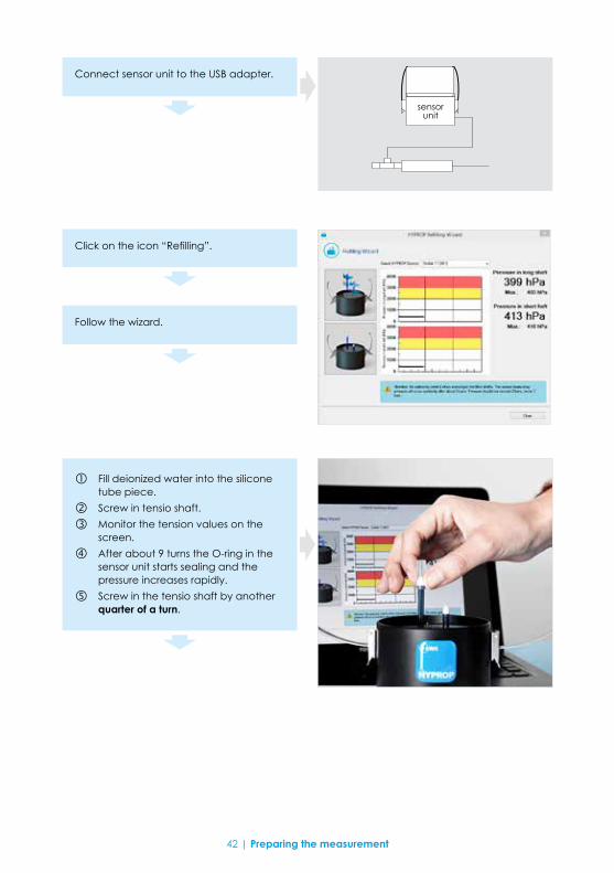
Connect sensor unit to the USB adapter.

Click on the icon “Refilling”.

Follow the wizard.

sensor unit

Fill deionized water into the silicone tube piece.

Screw in tensio shaft.

Monitor the tension values on the screen.

After about 9 turns the O-ring in the sensor unit starts sealing and the pressure increases rapidly.

Screw in the tensio shaft by another quarter of a turn.


Repeat all steps for the second tensio shaft.

When all steps are done click on “Close” and you get to the page where you opened the refilling wizard.

Note Be extremely cautious when you screw in the tensio shafts filled with water. The pressure that can damage the pressure sensor increases abruptly at about 9 turns. This pressure should not exceed 2000 hPa (200 kPa) – and in no case 3000 hPa (300 kPa).

Note If you open the wizard during a measurement the measuring process is interrupted. Therefore the wizard is closed automatically after 2 min and the measurement is continued.


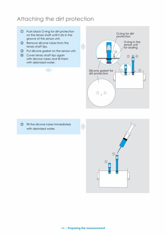
Attaching the dirt protection

Push black O-ring for dirt protection on the tensio shaft until it sits in the groove of the sensor unit.

Remove silicone tubes from the tensio shaft tips.

Put silicone gasket on the sensor unit.

Cover tensio shaft tips again with silicone tubes and fill them with deionized water.

Silicone gasket for dirt protection

O-ring for dirt protection

O-ring in the sensor unit for sealing

Fill the silicone tubes immediately

with deionized water.


Connect sensor unit to the USB adapter.

Click on the "Refilling" icon.

Function check

sensor unit

HYPROP USB adapter

Checking the zero point

Put a drop of water on the ceramic tip of the tensio shaft. By this zero potential exists.

The screen should indicate zero pressure for both tensio shafts.


Keep a syringe filled with deionized water on hand.

Remove silicone tube from the long tensio shaft and dry the ceramic tip with a paper towel.

Use a sheet of cardboard and fan air to the ceramic. Monitor the pressure display on the screen.

The pressure should increase up to the atmospheric air pressure minus 100 hPa (10 kPa) within 15 seconds.

Checking the speed of response

As soon as the pressure has reached the atmospheric air pressure (e.g. 100 hPa or 10 kPa) wet the ceramic immediately with deionized water.

Otherwise air may enter the tensio shaft and the degassing process has to be repeated!

Put silicone tube on tensio shaft and

fill up.

Repeat steps to for the short tensio shaft.

Note If the pressure does not rise to tensions close to atmospheric air pressure minus 100 hPa (10 kPa), highly likely air is in the tensio shaft. Then degassing the water in the sensor unit has to be repeated!Other potential failures:• tensio shaft does not sit tightly on the O-ring,• tensio shaft is clogged (e. g. by oils from fingers)• O-ring of the tensio shaft is worn out.

Checking the end vacuum


Assembling the sensor unit and the soil sample

Drilling the holes

Set tensio shaft adapter onto the saturated soil sample in the tray. The small hole should be above the sample ring number. This makes finding the right position easier when the sensor unit and the soil sample are assembled.

Use the tensio shaft auger to drill the holes. Carefully drill in 10 mm steps and make sure the soil sample is not compressed.

Fill drill holes with water to make sure air will not be pressed into the soil sample during assembly.

Sample ring number

Small hole


Set the sensor unit cautiously upside down onto the soil sample. Make sure, no air gaps are generated and the soil is not compressed.

Turn the whole test assembly upside down.

Remove saturation plate and nonwoven cloth.

Fix soil sample with the clips.

Carefully clean the sample ring and clips and dry them. Otherwise water and dirt will be weighed too.

The soil sample is now ready to be measured.


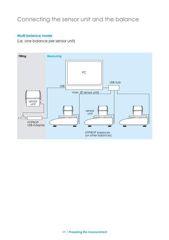
Connecting the sensor unit and the balance

Multi balance mode (i.e. one balance per sensor unit)

Filling Measuring

USBUSB hub

max. 20 sensor units

sensor unit

sensor unit

PC

HYPROP USB-Adapter

HYPROP balances (or other balances)


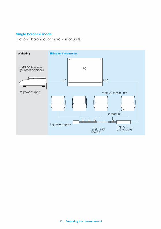
Single balance mode (i.e. one balance for more sensor units)

Weighing

HYPROP balance (or other balance)

to power supply

to power supply

USB USB

Filling and measuring

PC

max. 20 sensor units

tensioLINK® T-piece

HYPROP USB adapter

sensor unit


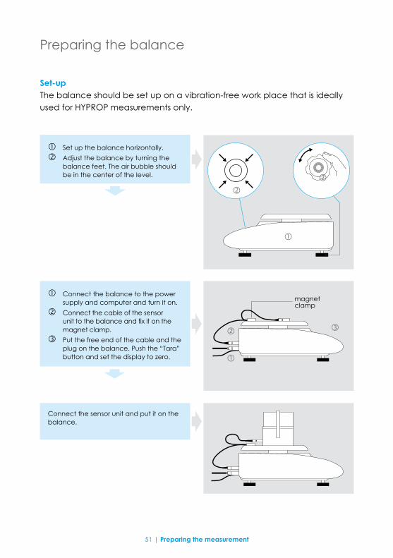
Set-up

Preparing the balance

The balance should be set up on a vibration-free work place that is ideally used for HYPROP measurements only.

Set up the balance horizontally.

Adjust the balance by turning the balance feet. The air bubble should be in the center of the level.

Connect the balance to the power supply and computer and turn it on.

Connect the cable of the sensor unit to the balance and fix it on the magnet clamp.

Put the free end of the cable and the plug on the balance. Push the “Tara” button and set the display to zero.

Connect the sensor unit and put it on the balance.

magnet clamp


Note

The both ends of the sensor unit cable must not touch each other as this would lead to noisy measurements.


Adjusting

For precise measurements the balance needs to be adjusted to the local conditions:• when it has been set up initially• after a change of position• after a temperature change. We recommend adjusting the balance also every 4 weeks when the balance is in measuring operation. For its adjustment the balance is equipped with an adjusting weight.

Remove magneto cable and HYPROP sensor unit.

Connect balance to the power supply and turn it on.

Push and hold button until S.A. CAL appears.

Func

S.A. CAL

Push both buttons at the same time and release them. VaIT

CAL. 0The readout flashes.

CAL

CAL. onThe zero point is saved.

CAL


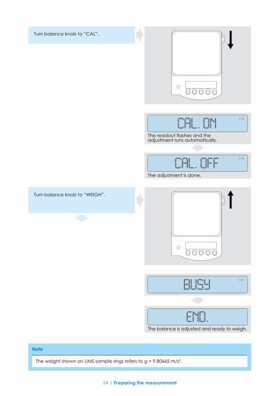
Turn balance knob to “CAL”.

CAL. onThe readout flashes and theadjustment runs automatically.

CAL

CAL. oFFThe adjustment is done.

CAL

Turn balance knob to “WEIGH”.

End.The balance is adjusted and ready to weigh.

buSYCAL


Note The weight shown on UMS sample rings refers to g = 9.80665 m/s².

Function Display Adjustment

Bar graph On

Toleranzwiegung Off

NullabgleichAutomatic zero point correction activated.

Automatic shut off after 3 min (recharge able battery operation)

On

Readout speed medium speed

Vibration filter medium sensitivity

Interface 6 digit data format

1 b.G. 1

2 SEL 0

3 A.0 1

4 A.P. 1

5 rE. 3

6 S.d. 2

7 I.F. 1

Default settings


Multi balance mode (one balance per sensor unit)

Measuring

Click on the "Show devices" icon.

If the balance does not show on the screen check if balance is turned on.

Click on the "Measurement wizard" icon.

Push start button.

Enter the following data – either via the wizard or directly in the manager:- measuring mode,- measuring unit,- name of the soil sample,- sample ring type and- balance type.

After entering the data the key legend changes to “Start”.

Actual and maximumtension value of theupper and lower tensio shaft in minute cycle)

Actual sample mass (in minute cycle)

!

56 | Measuring

Note The magneto cable from the balance to the magnet clamp must lie freely as a loop without touching anything. Before you start weighing wait for at least 5 minutes to let the cable tension release.

Single balance mode (one balance for more sensor units)

Click on the "Show devices" icon.

Push start button.

After filling in the data the key legend changes to “Start”.

Actual and maximum tension value of the upper and lower tensio shaft (in minute cycle)

!

If the balance does not show on the screen check if balance is turned on.

Click on the "Measurement wizard" icon.

Enter the following data – either via the wizard or directly in the manager:- measuring mode,- measuring unit,- name of the soil sample,- sample ring type and- balance type.

57 | Measuring

Note The magneto cable from the balance to the magnet clamp must lie freely as a loop without touching anything. Before you start weighing wait for at least 5 minutes to let the cable tension release.

Weighing the sample mass

Remove plug from sensor unit.

Follow the instructions on the screen.

The system identifies automatically the sen-sor unit having been put on the balance.

A menu opens on the screen showing information about the status and the weighing routine.

In the single balance mode we recommend to weigh the sample mass twice a day.

Note Only one sensor unit may be disconnected. Please do not pull the magneto cable but use the serrated area of the plug instead.

The number of samples is limited to 20.

Actual sample mass

The menu leads you through the weighing procedure.

Disconnect sensor unit from the balance and connect it again to the T-piece of the tensioLINK®. This function is supported with a menu.

Note If you run more sensor units with one balance the magneto cable is not needed.

58 | Measuring

Optimal measuring curve

Every measurement runs in 4 phases provided that tensio shafts and sensor unit are filled air free.

Phase 1, regular measurement rangeTension value curve rises up without flattening until it reaches the boiling point of the water.

Phase 2, boiling delay phaseIn the ideal case – when the system is filled completely air free – the tension value rises up to the boiling delay area (above the ambient air pressure). This is nice to have but in general not necessary for the evaluation.

Phase 3, Cavitation phaseWater vapor is generated in the tensio shaft and the tension value drops abruptly down to the boiling point. After this the tension value decreases only slightly.

Phase 4, Air entry phaseThe tension value again drops abruptly – now to zero, as air penetrates the ceramic. The air entry point is a material characteristic of the ceramic and amounts to about 8800 hPa (880 kPa). This point can also be used for the evaluation.

59 | Optimal measuring curve

0

1000

2000

Phase 1 Phase 2 Phase 3 Phase 4

The four phases using one tensio shaft as examplemeasured values interpolated values

time

tension [hPa or kPa]

air entry point of the tensio shaft

actual atmospheric air pressure

regular measurement range cavitation air entryboiling delay


0

1000

2000

Notes on suboptimal measuring curves

Often the optimal measuring curve up to the boiling delay cannot be achie-ved. The curves then look similar to the example below. But even these cur-ves can be used for an evaluation. In the chapter “Addendum” you find exemplary measuring curves of various soils.

air entry

Tensio top Tensio bottom


time


0

Finishing a measurement

You can finish a measurement in three ways:1. You stop when the upper tensio shaft has reached the cavitation phase

(see illustration 1). Then you do not use the air entry point.2. You are willing to use the air entry point. Then there are two possibilities:a) The air entry point of the first tensio shaft has been reached and the second

tensio shaft is still in the regular measurement range (phase 1) or in boiling delay (phase 2). In this case HYPROP can calculate the medial value of the Tensio top and Tensio bottom curve (see illustration 2).

b) When the air entry point of the first tensio shaft has been reached and the second tensio shaft is still in the cavitation phase (phase3), the medial value of the two cannot yet be calculated. Then please wait until the air entry point of the second tensio shaft has been reached (see illustration 3).

StopTensio Top Tensio Bottom

62 | Finishing a measurement

Illustration 1

time


0

air entry point


Illustration 2


time


0

air entry point 1 air entry point 2


In either case click the “Stop” button to finish the measurement.

After this you can have the software HYPROP FIT evaluate the measuring values. For this please see the manual using this link:www.ums.muc.de/static/Manual_HYPROP-FIT.pdf

Illustration 3


time


HYPROP needs the dry weight of the soil sample to be able to calculate the volumetric water content based on the weight reduction. Therefore the sample has to be weighed after the measuring campaign.

Note If the soil sticks too tightly to the sensor unit (which is often the case with clayey soils) put the sample ring with the sensor unit upside down in water. The water level should be above the rim of the sample ring. If necessary leave it in the water over night. Then the sample ring can be removed more easily.

Determining the dry weight

Put the soil sample in a bowl (ideally in a heat resistant one, so that you can put it in the oven for drying).

Open the clips of the sensor unit.

Cautiously remove the sample ring. Do not tilt the sample ring. If you do so you may break the tensio shafts.

Collect the soil material completely in the bowl.

65 | Determining the dry weight

To determine the real water content of the soil the dry mass is weighed.

Weighing the dry mass

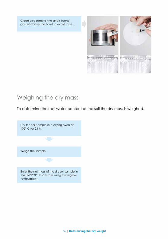
Dry the soil sample in a drying oven at 105° C for 24 h.

Weigh the sample.

Enter the net mass of the dry soil sample in the HYPROP FIT software using the register “Evaluation”.

Clean also sample ring and silicone gasket above the bowl to avoid losses.

66 | Determining the dry weight

Evaluating the measurement

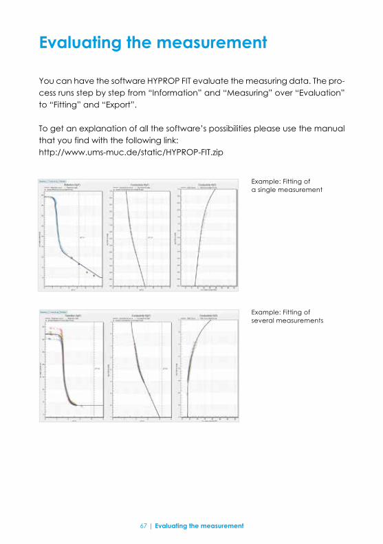
You can have the software HYPROP FIT evaluate the measuring data. The pro-cess runs step by step from “Information” and “Measuring” over “Evaluation” to “Fitting” and “Export”.

To get an explanation of all the software’s possibilities please use the manual that you find with the following link: http://www.ums-muc.de/static/HYPROP-FIT.zip

Example: Fitting of a single measurement

Example: Fitting of several measurements

67 | Evaluating the measurement

Problem How to solve it

1. The tensio shaft is dry. Fill tensio shaft either by means of a syringe or vacuum pump with deionized water (see chapter “Preparing a measurement”.

2. You identify bubbles in the tensio shafts.

Repeat filling. If this does not help: try to detect leakage (e.g. red O-ring of the tensio shaft) and fix it.

3. The tension value rea-ches only 500 … 700 hPa (50 … 70 kPa) and drops then.

a) Tensio shaft has not been filled air free (how to fix it see above). b) Red O-ring of the tensio shaft does not seal properly. Check and if necessary replace O-ring (see chapter “Cleaning and maintenance”).

4. The Tensio bottom stops at 200 … 700 hPa (20 … 70 kPa) and drops then.

Potential reasons: a) The soil sample is disrupted horizontally and was initially filled with water but later on with air which works as a capillary block. b) Same problems as #3.

5. The tension value ex- ceeds the value of the atmospheric pressure (e.g. 1000 hPa or 100 kPa).

This is no fault but the physical effect of boiling delay. Thus you can measure with HYPROP beyond the “normal” measuring range.

6. Measuring data are no longer recorded.

a) Check connection to the USB port. b) Change energy management of your computer to “continuous operation” (typical when using a lap top).

7. At the beginning of a measurement the Ten-sio bottom “overtakes” the Tensio top

Maybe the tensio shafts have been interchanged. There is no need to interrupt the measurement as you can correct the mea-suring values in HYPROP-FIT.

8. In the “Single balance mode” the software does not find any sensor units.

Disconnect the sensor units one by one and have the software show the device tree. Probably one or more sensor units have the same address. Change addresses (see chapter “Preparing a measurement”).

9. wYou monitor readout values of 4000 hPa (400 kPa).

The pressure sensors have been destroyed. The sensor unit must be checked. Please send it/them to UMS or your local dealer. We will repair it fast and at cost-efficiently.

68 | Trouble shooting

Trouble shooting

Cleaning and maintenance

Do not remove the tensio shafts.

Close lid of the plug.

Clean sensor unit properly upside down under running water.

Dry with cloth.

When the sensor unit is clean unscrew ten-sio shafts by about 5 turns and clean them again. Then remove tensio shafts.

Cleaning the sensor unit

The sensor unit meets the protection class IP65 and therefore can be cle-aned under running water.

After removing the tensio shafts keep sensor unit upside down and wash residu-al soil particles away.

Note

Always clean the sensor unit upside down using a wash bottle to make sure no soil particles enter the sensor unit.

69 | Cleaning and maintenance

When during the tension rise the values of a tensio shaft flatten significantly or even drop before reaching the vacuum (at about 800 hPa or 80 kPa) this indicates a leakage. In this case change the red O-rings in the sensor unit.

Changing the O-rings in the sensor unit

Use fine pointed tweezers to pierce the O-ring and pick it.

Take the spare O-rom from the service pack. Do not pierce it.

Put O-ring into the hole and let it “snap” into the groove on the bottom.

If the O-ring does not snap in itself screw in the tensio shaft cautiously.


Note

Do not stick the tweezers tip into the hole of the sensor unit. You may damage the pressure sensor.

Empty carefully sensor unit and tensio shafts.

Protect sensor unit from dust.

Store sensor unit and tensio shafts dry.

Storage

If you do not use the HYPROP over a longer period of time make sure to avoid any algae growth.


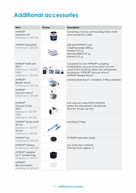
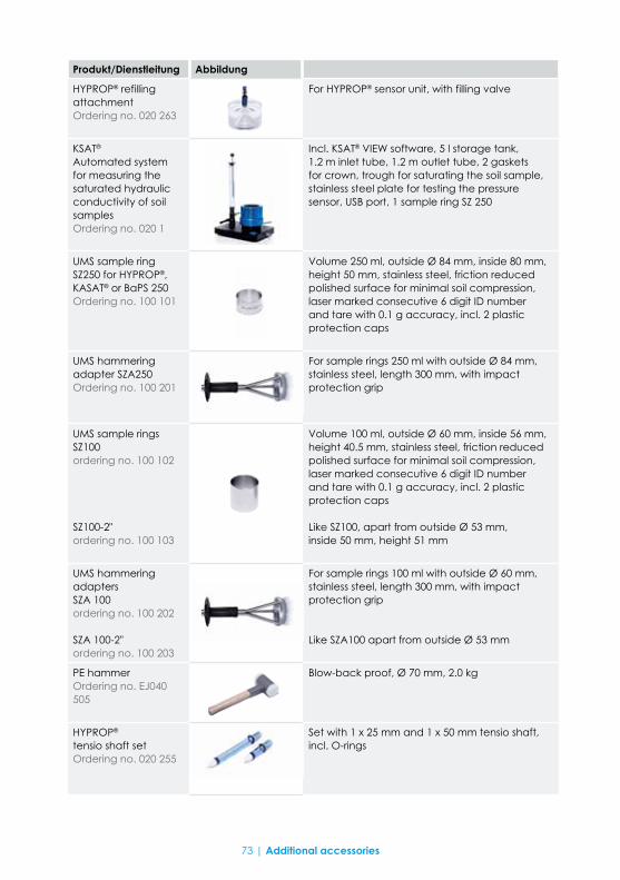
Additional accessories

Item Picture Description

HYPROP® extension set Ordering no. 020 203

Consisting of sensor unit including tensio shafts and connection cable

HYPROP® BALANCEOrdering no. 020 204

USB and HYPROP® port, weighing range 2200 g, readout 0.01 g, reproducibility 0.01 g, linearity 0.01 g

HYPROP® Refill Unit 230 V ordering no. 020 257 110 V ordering no. 020 258

Complete for one HYPROP® consisting of laboratory vacuum pump (end vacuum value 8 hPa (0.8 kPa)) below the atmospheric air pressure, HYPROP® Vacuum Mount, HYPROP® Beaker Mount

HYPROP® Beaker MountOrdering no. 020 262

Stainless steel mount, 2 beakers, 4 filling adapters

HYPROP® Vacuum MountOrdering no. 020 268

-

HYPROP® Vacuum Pump 230 V ordering no. 020 259 110 V ordering no. 020 260

End vacuum value 8 hPa (0.8 kPa) below the atmospheric air pressure, 20 l/min, for lab use only

HYPROP® tensio shaft 50 mmordering no. 020 277 25 mmordering no. 020 281

Including O-rings

HYPROP® SatOrdering no. 020 253

HYPROP® saturation plate

HYPROP® TrainingOrdering no. 020 254

Incl. instruction material, training hours: approx. 4

HYPROP® Adapter for 2” sample rings Ordering no. 020 271

HYPROP® Silicone Gasket Ordering no. 020 267

72 | Additional accessories

Produkt/Dienstleitung Abbildung

HYPROP® refilling attachment Ordering no. 020 263

For HYPROP® sensor unit, with filling valve

KSAT®

Automated system for measuring the saturated hydraulic conductivity of soil samples Ordering no. 020 1

Incl. KSAT® VIEW software, 5 l storage tank, 1.2 m inlet tube, 1.2 m outlet tube, 2 gaskets for crown, trough for saturating the soil sample, stainless steel plate for testing the pressure sensor, USB port, 1 sample ring SZ 250

UMS sample ring SZ250 for HYPROP®, KASAT® or BaPS 250 Ordering no. 100 101

Volume 250 ml, outside Ø 84 mm, inside 80 mm, height 50 mm, stainless steel, friction reduced polished surface for minimal soil compression, laser marked consecutive 6 digit ID number and tare with 0.1 g accuracy, incl. 2 plastic protection caps

UMS hammering adapter SZA250 Ordering no. 100 201

For sample rings 250 ml with outside Ø 84 mm, stainless steel, length 300 mm, with impact protection grip

UMS sample rings SZ100ordering no. 100 102

SZ100-2"ordering no. 100 103

Volume 100 ml, outside Ø 60 mm, inside 56 mm, height 40.5 mm, stainless steel, friction reduced polished surface for minimal soil compression, laser marked consecutive 6 digit ID number and tare with 0.1 g accuracy, incl. 2 plastic protection caps

Like SZ100, apart from outside Ø 53 mm, inside 50 mm, height 51 mm

UMS hammering adapters SZA 100ordering no. 100 202

SZA 100-2"ordering no. 100 203

For sample rings 100 ml with outside Ø 60 mm, stainless steel, length 300 mm, with impact protection grip

Like SZA100 apart from outside Ø 53 mm

PE hammer Ordering no. EJ040 505

Blow-back proof, Ø 70 mm, 2.0 kg

HYPROP® tensio shaft set Ordering no. 020 255

Set with 1 x 25 mm and 1 x 50 mm tensio shaft, incl. O-rings

73 | Additional accessories

Theory

Preliminary note HYPROP (HYdraulic PROPerty analyser) is a device to measure hydraulic key functions of soil samples in a comfortable and reliable way by using an evaporation experiment.

Wind (1966) developed the evaporation method in the mid-sixties. For this 5 tensiometers were put in a soil sample. The sample was set on a balance and over the evaporation process the tensions and the mass change of the samp-le were measured in time intervals. Based on these data the water retention function and the unsaturated hydraulic conductivity in the range between saturation and maximum 500 hPa (50 kPa) were calculated by means of an iteration process. Schindler (1980) simplified this method. He used only 2 ten-siometers and simplified the evaluation procedure. HYPROP is working based on this method. The method was tested several times and its fitness for use was proven by scientific analysis (Wendroth et al., 1993, Peters and Durner, 2008; Peters et al., 2015). New research results yielded a further simplified measuring procedure (Schindler and Mueller, 2006) and an extended measuring range (Schindler et al., 2010a and Schindler et al., 2010b). Using the HYPROP one can today measure simultaneously the water retention curve and the unsaturated hydraulic conductivity function in the range between water saturation and close to the permanent wilting point. The measuring time amounts – depen-ding on the soil – from 2 days (clay samples) to maximum 10 days (peat and sand samples). Additionally the dry bulk density of the sample is determined.

The measurement and evaluation can be run in two modes. In the multi ba-lance mode (one balance per sample) the lab employees’ work effort is limi-ted to set up and take away the samples. In the single balance mode (one balance for more samples) up to 20 samples can be measured in parallel. In this mode it is necessary to put the probes manually on the balance twice a day. This takes about 15 s per sample and weighing. The measurement of the tension runs automatically. The software HYPROP-VIEW enables a comforta-ble data logging and storage. The software HYPROP-FIT provides the same comfort for data evaluation, fitting and export of the hydraulic key functions.The hysteresis of the saturation and dewatering characteristics of the hydrau-lic key functions is described in Schindler et al. (2015).

74 | Theory

Measurements considering the shrinkage characteristics of the soil sample are described in Schindler et al., 2015. Comparing the measuring results of HYPROP and classical methods (sand box, kaolin box, pressure pot) demons-trated good congruence (Schelle et al., 2010, 2011, 2013a, b; Schindler et al., 2012). Systematical differences could not be found.

Measuring method HYPROP® measures the water tension/water content relation (“retention curve”, “pF/WC curve”) of a soil sample. It also measures how the unsaturated hydraulic conductivity depends on the water tension/content (“Ku curve”). This is based on the evaporation method according to Wind (1968) in Schindler’s model (1980).

With this method two tensiometers are positioned in two depths of a soil samp-le sitting in a sample ring. The plane in the middle between the two tensiome-ters is identical with the horizontal symmetry plane of the column. The sample is saturated with water, basally closed and set on a balance. The soil surface is open to the ambient atmosphere so that the soil water can evaporate. HYPROP measures the water tension in two horizons of the soil sample over the evaporation process by means of two vertical tensio shafts (similar to T5 tensiometers) . The change of the sample mass over time is determined by weighing. The medial pF value of the sample is calculated based on the aver-age value of the two tensions. The medial water content is calculated based on the mass change. This results in one measuring value per point in time for the pF/WC curve.

The evaporation rate results from the mass differences, based on this the vo-lume flow is calculated at each point in time. The values of the hydraulic conductivity with increasing desiccation are a result of how well the soil can transport this water to the top where it evaporates. If the conductivity is poor the soil on top dries out whereas it remains wet on the bottom. So the upper tensio shaft indicates “drier” than the lower tensio shaft which is still “wet”. If the conductivity is good the whole water of the sample is evaporated and bother tensio shafts indicate almost the same values. The detailed calculation basics of the method as well as the check of its validity are explained in Peters and Durner (2008) and Peters et al. (2015).

75 | Theory

The terms tension, matrix potential, water tension and pF value refer to the same physical value: they describe the energy that attracts water mole-cules – to pores capillary or to soil particles adhesively. Plants e.g. must overcome this binding energy (or attraction force), to suck water from the soil matrix.

The water is under tension in the soil. This tension or attraction force can be directly measured as a vacuum of the water compared to the atmospheric pressure. So for the measurement water in the tensio shaft is “offered” to the soil. The soil sucks it with the same force as it retains the water. As the soil has a capillary contact to the water in the tensio shaft through the pores of the ceramic the pressures of the water in the soil and in the tensio shaft finally match.

As the tensio shaft water is locked air tight, it cannot flow into the soil before the soil is so dry and accordingly the vacuum is so high that the first pore layer gets empty. This vacuum (tension) can be measured with a pressure sensor. If the vacuum is strong enough to suck the small pores empty the water entry point has been reached: air enters the tensio shaft, the pressure rises up to the atmospheric pressure and the pressure read out drops to zero.

The matrix potential is the negative value of the tension. It is often expressed in hPa or kPa. In the soil science also the pressure head is used, e.g. in the unit “cm water column”. The pF value is the decimal logarithm of a wa-ter column in cm. A soil water tension of -100 hPa is equivalent to a water column of approximately* 100 cm. So its pF value is 2.0

The terms retention function, pF curve and pF/WC characteristics mean the same. They describe a soil characteristic dependent on the binding energy (pF value, water tension) and on the water content (WC). As an example: Sand can retain only little water, clay a lot. At or near saturation sand con-ducts water very well, clay however poorly. Dry sand conducts water very poorly, compared to this clay is a bit better (water conducting horizons). Please see the following retention curves for comparison.

Explanation of terms

* as g = 9.81 m/s²

76 | Theory

Typical retention curve of sand.

Typical retention curve of loam.

77 | Theory

HYPROP measures the water tensions h1 and h2 (in hPa or kPa) in two mea-suring levels of the sample at certain points of time t being defined in the HYPROP-VIEW configuration. In the multi balance mode also the total mass of the sample is weighed (in g) at the same time. In the single balance mode the sample mass is weighed manually – usually twice a day. The software cal-culates the medial water content of the sample based on the sample mass minus all tare components (sensor unit, sample ring, dry mass of the soil). The dry mass of the soil can be determined after the measurement by drying the sample in an oven at 105 °C.

The measuring data are evaluated with the software HYPROP-FIT according to Schindler’s method (1980). The precise calculation of the water content needs the input of the soil’s dry mass. As long as the dry mass has not been entered HYPROP estimates the water content upfront. HYPROP-FIT calcula-tes based on linearization assumptions discrete points of the retention and the conductivity curves. For this in a first step the raw data are interpolated by Hermitian splines. This has the advantage that differing measuring times of tensions and water contents can be adjusted and the number of time points that are used for calculating data are fixed a priori. The default set in HYPROP-FIT is a calculation at 100 time points that are taken from the splines.

At every calculation time point a medial water content θi is calculated by di-viding the mass of the soil water by the volume of the soil body. Each of these points is assigned to a tension that is calculated from the measured and avera-ged tensions h1 and h2. Finally this procedure results in 100 points of the retention curve θi(hi). In order to calculate the conductivity function it is assumed that the water flow through a horizontal plane that lies exactly in the middle of the two tensio shafts (and thus in the symmetry plane of the column) between two time points ti-1 and ti is qi = 1/2 (∆Vi/∆ti )/A. With ∆Vi being the water reduction (in cm³) over the mass change, ∆ti the time interval between two calculation time points and A the cross-sectional area (in cm²) of the column. The data points for the hydraulic conductivity function are calculated by inverting Darcy’s equati-on: Ki (hi )= -qi /{(∆hi/∆z)-1}. With hi being the time- and space-averaged tension, ∆hi the difference of the two tensions at the two measuring levels, and ∆z the distance of the measuring levels (i. e. the height difference of the tensio shafts).

Generating discrete data points for retention and conductivity functions

78 | Theory

HYPROP-FIT filters the unreliable K(h) data pairs near saturation depending on the measuring accuracy of the tensio shafts (Peters and Durner, 2008). After this parametric functions θi(hi) and Ki(hi) are adjusted to the measuring points θ(h) and K(h) gained by non-linear optimization. In HYPROP-FIT the user can select the type of function; all usual models can be found (van Genuchten, 1980; Brooks and Corey, 1964; Kosugi, 1996; Fredlung-Xing, 1994) in uni- and bi-modal form as well as in a more sophisticated modelling as Peters-Durner-Iden (PDI) variant (Peters, 2013; Iden und Durner, 2014). You can find a com-plete description of the evaluation procedure as well as the models and the curve fitting in the HYPROP-FIT manual (http://www.umsmuc.de/static/Ma-nual_HYPROP.pdf) and in Peters et al., (2015).

79 | Theory

The θ(h) and K(h) functions are adapted simultaneously to the data points. This is essential as distinct parameters (i. e and n ) at van Genuchten/Mua-lem) influence the shape of both functions.

The adaption is accomplished by a non-linear regression under minimization of the sum of all assessed squares of the distance between data points and model forecast. However, the assumption the water content is spread out linear over the column is not always fulfilled in coarse, pored or structured soil. Therefore, the so called “integral fit” is applied for the adaption of the retenti-on function to avoid a systematic error (Peters and Durner, 2006). For details of the fitting procedure and data assessment please refer to Peters and Durner (2007, 2008) and Peters et al., (2015).

Parameter optimization

Additional notes

Three factors limit or extend the measuring range of the tensio shafts:• the air entry point• the water vapor pressure (boiling point)• the boiling delay.

This value is specific for a porous hydrophilic structure and depending on the contact angle and the pore size. The air entry point of the UMS tensio shafts is about 8.8 bars so it does not limit the measuring range.

At a temperature of 20°C the vapour pressure of water is 2.3 kPa above vacu-um. This means: If the atmospheric pressure is 100 kPa at 20°C the water will start to boil or vaporize as soon as the pressure drops below 2.3 kPa (= 97.7 kPa pressure difference). At this point the measuring range of the tensio shafts ends.

Please note that the atmospheric pressures announced by meteorological services are always related to sea level. However the true atmospheric pres-sure at an elevation of 500 meters above sea level is for example only 94.2 kPa (although 100 kPa are announced). In this case the measuring range at 20°C is limited to -91.9 kPa. Even if the soil gets drier and drier the tension shown by the readout will remain at this value. But as soon as the bubble point is rea-ched a spontaneous compensation with the atmospheric pressure occurs. Then air enters the tensio shaft and the readout will rapidly drop to zero.

Influences on the measuring range

The air entry point of the tensio shaft

Water vapor pressure

The ceramic has a pore size of r = 0.3 μm and therefore cannot block ions. Thus, an influence of osmosis on the measurements is negligible. If the tensio shaft is dipped into a saturated NaCl solution the readout will show 1 kPa for a short moment, then it will drop to 0 kPa again.

Osmotic effect

80 | Theory

Addendum

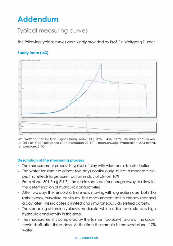
The following typical curves were kindly provided by Prof. Dr. Wolfgang Durner.

• The measurement process is typical of clay with wide pore size distribution• The water tensions rise almost two days continuously, but at a moderate slo-

pe. This reflects large pore fraction in clay of almost 10%• From about 50 hPa (pF 1.7), the tensio shafts are far enough away to allow for

the determination of hydraulic conductivities.• After two days the tensio shafts are now moving with a greater slope, but still a

rather weak curvature continues. The measurement limit is already reached a day later. This indicates a limited and simultaneously diversified porosity.

• The spreading of tension values is moderate, which indicates a relatively high hydraulic conductivity in this area.

• The measurement is completed by the (almost too early) failure of the upper tensio shaft after three days. At the time the sample is removed about 17% water.

Site: Wolfenbüttel; soil type: slightly sandy loam. Ls3 (S 35%, U 48%, T 17%); measurements in win-ter 2011 at "Geoökologische Labormethoden 2011", TUBraunschweig. Evaporation: 2,75 mm/d, temperature: 21°C

Typical measuring curves

Sandy loam (Ls3)

Description of the measuring process

81 | Addendum

• The relatively uniform decrease in the water content with increasing pF and the drop of the relatively flat K data is characteristic of clays having a wide pore size distribution.

• The addition of the data point on the bubble point of the ceramic tip (po-wer users only) fits very well with the independent, measured WP4 data points, and extends the range considerably.

• As a model to describe the data a bimodal function is needed.

Evaluation

82 | Addendum

Clayey silt (Ut3)

Site: Groß-Gleidingen near Braunschweig; soil type: clayey silt (S: 1%, U: 82%, T:17%); measurements: Prak-tikum Bodenphysik at TU Braunschweig, 2010. Evaporation: 14 mm/d using a fan. Temperature: 20°C

• The measurement process is typical of a very fine grained substrate.• The water tensions rise spontaneously immediately after the start of mea-

surement, steeply and continuously. This reflects a very small proportion of coarse pores. pF 2.0 is reached (under the given conditions with fan) after a few hours. The loss of water to pF 2 is only about 4%.

• The "spikes" at the beginning of the measurements shows the discontinuous access of air penetrating into the soil.

• From 100 hPa (pF 2.0), the first parallel tensio shafts are far enough away to allow for the determination of hydraulic conductivities.

• Both tensio shafts rise unabated with the passage of time and failed relatively soon. The clayey silt has few large middle pore, the finer middle pore region is in the time of failure still filled with water, the water content is therefore high.

• The spread of the tension values is moderate over the entire measuring process, which indicates a relatively high unsaturated conductivity.

• The measurement is completed due to the failure of the upper tensio shaft after less than one day. At this time the sample has lost about 20% water.


83 | Addendum

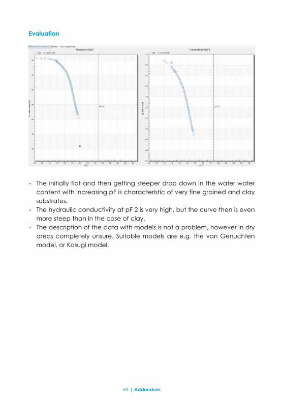
• The initially flat and then getting steeper drop down in the water water content with increasing pF is characteristic of very fine grained and clay substrates.

• The hydraulic conductivity at pF 2 is very high, but the curve then is even more steep than in the case of clay.

• The description of the data with models is not a problem, however in dry areas completely unsure. Suitable models are e.g. the van Genuchten model, or Kosugi model.

Evaluation

84 | Addendum

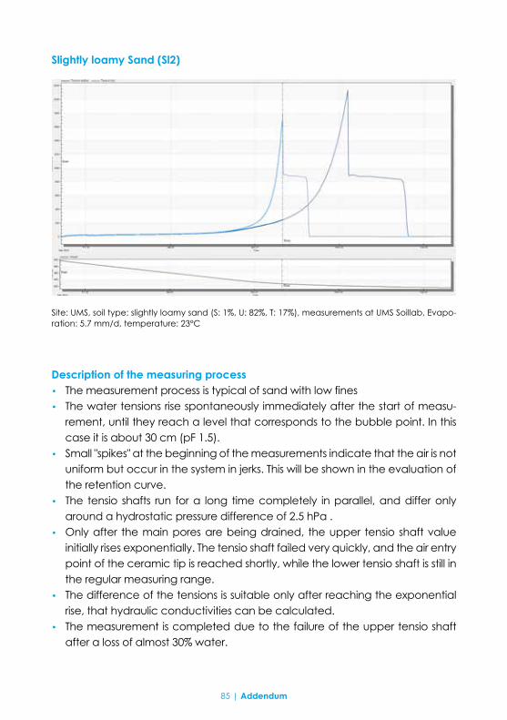
Slightly loamy Sand (Sl2)

Site: UMS, soil type: slightly loamy sand (S: 1%, U: 82%, T: 17%), measurements at UMS Soillab, Evapo-ration: 5.7 mm/d, temperature: 23°C

• The measurement process is typical of sand with low fines• The water tensions rise spontaneously immediately after the start of measu-

rement, until they reach a level that corresponds to the bubble point. In this case it is about 30 cm (pF 1.5).

• Small "spikes" at the beginning of the measurements indicate that the air is not uniform but occur in the system in jerks. This will be shown in the evaluation of the retention curve.

• The tensio shafts run for a long time completely in parallel, and differ only around a hydrostatic pressure difference of 2.5 hPa .

• Only after the main pores are being drained, the upper tensio shaft value initially rises exponentially. The tensio shaft failed very quickly, and the air entry point of the ceramic tip is reached shortly, while the lower tensio shaft is still in the regular measuring range.

• The difference of the tensions is suitable only after reaching the exponential rise, that hydraulic conductivities can be calculated.

• The measurement is completed due to the failure of the upper tensio shaft after a loss of almost 30% water.


85 | Addendum

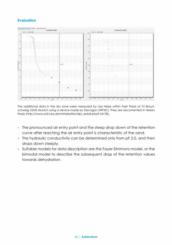
The additional data in the dry zone were measured by Lisa Heise within their thesis at TU Braun-schweig /UMS Munich using a device made by Decagon (WP4C). They are documented in Heise's thesis (http://www.soil.tubs.de/mitarbeiter/dipl_detail.php? id=78).

• The pronounced air entry point and the steep drop down of the retention curve after reaching the air entry point is characteristic of the sand.

• The hydraulic conductivity can be determined only from pF 2.0, and then drops down steeply.

• Suitable models for data description are the Fayer-Simmons model, or the bimodal model to describe the subsequent drop of the retention values towards dehydration.

Evaluation

86 | Addendum

Pure fine and middle sand (Ss)

Material: packed quartz sand particle size: 0.1 bis 0.3 mm, soil type: sandy sand (S: 100%, U: 0%, T: 0%), site: Bodenphysikalisches Labor, TU Braunschweig, evaporation: 1.4 mm/d, temperature: 22°C

• The measurement process is typical of sand with narrow particle size distri-bution and without fines

• The tension rise spontaneously immediately after the start of measurement, until they reach a level that corresponds to the bubble point. In this case it is about 50 cm (pF 1.7).

• The tensio shafts run for a long time completely in parallel, and differ only around a hydrostatic pressure difference of 2.5 hPa.

• After draining the main pore portion the tensio shaft value of the upper ten-sio shaft rises extremely steep. The failure of the tensio shaft is now very quick.

• The lower tensio shaft is at the end of the measurement still completely unaffected by the extreme dehydration front, the difference of water ten-sions is very high.

• Hydraulic conductivities can be calculated only for a short period of time.• The measurement is completed due to the failure of the upper tensio shaft

after removal of 35% water


87 | Addendum

• The very sharply defined bubble point and the extremely steep drop in the retention curve after reaching the air entry point is characteristic of pure sand with a uniform grain size.

• The hydraulic conductivity can be determined only within a very narrow tension intervall, and drops down very steeply.

• Suitable models are the data description Brooks Corey model, the van Genuchten model of free parameter m or the Simmons-Fayer model.

Evaluation

Standard pF curves

Standard pF curves (courtesy of Dr. Uwe Schindler, ZALF Muencheberg)

88 | Addendum

Sample treatment for WP4 measurements after a HYPROP measurement

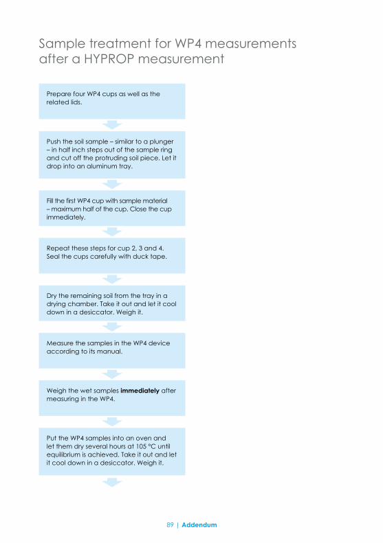
Push the soil sample – similar to a plunger – in half inch steps out of the sample ring and cut off the protruding soil piece. Let it drop into an aluminum tray.

Prepare four WP4 cups as well as the related lids.

Fill the first WP4 cup with sample material – maximum half of the cup. Close the cup immediately.

Repeat these steps for cup 2, 3 and 4. Seal the cups carefully with duck tape.

Measure the samples in the WP4 device according to its manual.

Weigh the wet samples immediately after measuring in the WP4.

Dry the remaining soil from the tray in a drying chamber. Take it out and let it cool down in a desiccator. Weigh it.

Put the WP4 samples into an oven and let them dry several hours at 105 °C until equilibrium is achieved. Take it out and let it cool down in a desiccator. Weigh it.

89 | Addendum

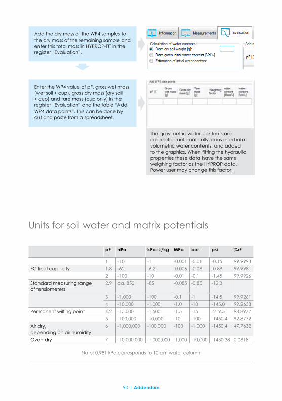
Units for soil water and matrix potentials

pF hPa kPa=J/kg MPa bar psi %rF

1 -10 -1 -0.001 -0.01 -0.15 99.9993

FC field capacity 1.8 -62 -6.2 -0.006 -0.06 -0.89 99.998

2 -100 -10 -0.01 -0.1 -1.45 99.9926

Standard measuring range of tensiometers

2.9 ca. 850 -85 -0,085 -0.85 -12.3

3 -1,000 -100 -0.1 -1 -14.5 99.9261

4 -10,000 -1,000 -1.0 -10 -145.0 99.2638

Permanent wilting point 4.2 -15,000 -1,500 -1.5 -15 -219.5 98.8977

5 -100,000 -10,000 -10 -100 -1450.4 92.8772

Air dry, depending on air humidity

6 -1,000,000 -100,000 -100 -1,000 -1450.4 47.7632

Oven-dry 7 -10,000,000 -1,000,000 -1,000 -10,000 -1450.38 0.0618

Note: 0.981 kPa corresponds to 10 cm water column

90 | Addendum

Add the dry mass of the WP4 samples to the dry mass of the remaining sample and enter this total mass in HYPROP-FIT in the register “Evaluation”.

Enter the WP4 value of pF, gross wet mass (wet soil + cup), gross dry mass (dry soil + cup) and tare mass (cup only) in the register “Evaluation” and the table “Add WP4 data points”. This can be done by cut and paste from a spreadsheet.

The gravimetric water contents are calculated automatically, converted into volumetric water contents, and added to the graphics. When fitting the hydraulic properties these data have the same weighing factor as the HYPROP data. Power user may change this factor.

Technical data

Facts and figures

Sensor unit

Material Dimensions

Fiber glass reinforced PolyamideHeight 60 mm, Ø 80 mm

Tensio shafts

CeramicShaft materialTotal length

Al2O3 sinter, bubble point > 200 kPa; Ø 5 mmAcrylic glass; Ø 5 mmSmall tensio shaft: 31 mmBig tensio shaft: 56 mm

Measuring range

Pressure transducerTemperature

-3.0 … 3000 hPa (-0.3 … 300 kPa), electronic-30 … 70 °C

Accuracy

PressureTemperature

± 2,5 hPa / d = 0,05 hPa (+100 ... -500 hPa)± 0,2 K (at -10 … 30 °C) / d = 0,01 K

Power supply

VoltageCurrent

6 … 10 V DC6 mA nominal, 15 mA max.

Chemical resistance

pH range pH3 … pH10,

Limited to media that do not affect silicon, fluorosilicone, EPDM, PMMA or polyetherimide

Protection

Housing with covered plug IP65 splash water proof

Sensor units

Number of sensor units supported by tensioLINK

20

HYPROP balance

Connection to computerWeighing rangeReadoutReproducibilityLinearityAdjustment

USB2200 g0.01 g0.01 g0.01 ginternally

91 | Facts and figures

Literature cited

• Brooks, R. H. and Corey, A. T. (1964): Hydraulic properties of porous media. Hydrology Paper 3. Colorado State University, Fort Collins, Colorado.

• Fredlund, D. G., & Xing, A. (1994): Equations for the soil-water cha-racteristic curve. Canadian geo-technical journal, 31(4), 521-532.

• Iden, S.C., and W. Durner (2014): Comment to “Simple consistent models for water retention and hydraulic conductivity in the complete moisture range” by A. Peters., Water Resour. Res., 50, 7530–7534.

• Kosugi, K. I. (1996): Lognormal distribution model for unsatura-ted soil hydraulic properties. Wa-ter Resources Research, 32(9), 2697-2703.

• Peters, A. and Durner, W. (2006): Improved estimation of soil wa-ter retention characteristics from hydrostatic column experiments. Water Resources Research 42 (11).

• Peters, A. and Durner, W. (2008): Simplified Evaporation Method for Determining Soil Hydraulic Properties. Journal of Hydrology 356 (1-2): 147– 162.

• Peters, A. and Durner, W. (2007): Optimierung eines einfachen Verdunstungsverfahrens zur Be-stimmung bodenhydraulischer Eigenschaften. Mitteilungen der Deutschen Bodenkundlichen Gesellschaft 110 (1): 125-126.

• Peters, A. (2013): Simple consis-tent models for water retention and hydraulic conductivity in the complete moisture range, Water Resour..Res., 49, 6765–6780.

• Peters, A., S.C. Iden, and W. Durner (2015): Revisiting the simplified evaporation method: Identification of hydraulic func-tions considering vapor, film and corner flow. Journal of Hydrolo-gy, in press.

92 | Literature cited

Note If you want to cite this manual please use the following information: UMS (2015): Manual HYPROP, Version 2015-01, 96 pp. UMS GmbH, Gmunder Straße 37, Munich, Germany.URL http://ums-muc.de/static/Manual_HYPROP.pdf

• Schelle, H., Iden, S. C., Peters, A. and Durner, W. (2010): Analysis of the agreement of soil hydraulic properties obtained from mul-tistep-outflow and evaporation methods. Vadose Zone Journal 9 (4): 1080-1091.

• Schelle, H., Iden, S. C. and Durner, W. (2011): Combined transient method for determining soil hydraulic properties in a wide pressure head range. Soil Scien-ce Society of America Journal 75 (5): 1-13.

• Schelle, H., Heise, L., Jänicke, K. and Durner, W. (2013a): Wasser-retentionseigenschaften von Bö-den über den gesamten Feuchte-bereich - ein Methodenvergleich. - In: Beiträge zur 15. Lysimeterta-gung am 16. and 17. April 2013, HBFLA Raumberg-Gumpenstein.

• Schelle, H., Heise, L., Jänicke, K. and Durner, W. (2013b): Water retention characteristics of soils over the whole moisture range: a comparison of laboratory me-thods. European Journal of Soil Science 64 (6): 814-821.

• Schindler, U. (1980): Ein Schnell-verfahren zur Messung der Was-serleitfähigkeit im teilgesättigten Boden an Stechzylinderproben. Archiv für Acker- und Pflanzen-bau und Bodenkunde 24 (1): 1-7.

• Schindler, U. and Müller, L. (2006): Simplifying the evapora-tion method for quantifying soil hydraulic properties. Journal of Plant Nutrition and Soil Science 169 (5): 623-629.

• Schindler, U., Durner, W., von Unold, G. and Müller, L. (2010a): Evaporation method for mea-suring unsaturated hydraulic properties of soils: Extending the measurement range. Soil Scien-ce Society of America Journal 74 (4): 1071-1083.

• Schindler, U., Durner, W., von Unold, G., Müller, L. and Wieland, R. (2010b): The evapo-ration method: Extending the measurement range of soil hy-draulic properties using the air‐entry pressure of the ceramic cup. Journal of Plant Nutrition and Soil Science 173 (4): 563-572.

• Schindler, U., Doerner, J. and Müller, L. (2015): Simplified me-thod for quantifying the hydrau-lic properties of shrinking soils. Journal of Plant Nutrition and Soil Science 178 (1): 136–145.

• UMS (2015): HYPROP-Fit User Manual. UMS GmbH, Gmun-der Str. 37, 81379 München, Germany, 2015. URL http://www.ums.muc.de/static/Manual_HYPROP-FIT.pdf.


• Van Genuchten, M. T. (1980): A closed-form equation for predic-ting the hydraulic conductivity of unsaturated soils. Soil Science Society of America Journal 44: 892-898.

• Wind, G.P. (1968): Capillary con-ductivity data estimated by a simple method. p.181–191. In R.E. Rijtema and H. Wassink (ed.) Water in the Unsaturated Zone: Proc. UNESCO/IASH Symp., Wa-geningen, the Netherlands.

Notes


Notes

95 | Notes

UMS GmbHGmunder Str. 37

81379 Munich

Phone +49 (0) 89 / 12 66 52 - 0Fax +49 (0) 89 / 12 66 52 - 20

[email protected]

© 2015 UMS GmbH, Munich, Germany, www.ums-muc.dePrint #: HYPROP vers2015_01 Subject to modifications and amendments without notice.HYPROP®, HYPROP-VIEW® und HYPROP-FIT® are registered trademarks of UMS GmbH, Munich, Germany.Printed on paper made of chlorine-free bleached pulp.

Documents

Operation Manual HYPROP - METERlibrary.metergroup.com/Manuals/UMS/Hyprop_Manual.pdf · Operation Manual HYPROP ... In case a balance does not show, check ... Short cuts to key functions