Embed Size (px)
Citation preview
CHAPTER IV
STABILITY
41 THE STABILITY PROBLEM
The discussion of feedback systems presented up to this point has tacitly
assumed that the systems under study were stableA stable system is defined in general as one which produces a bounded output in response to any
bounded input Thus stability implies that
I vo(t) dt lt M lt o (41)
for any input such that
f vr(t) dt lt N lt o (42)
If we limit our consideration to linear systems stability is independent of
the input signal and the sufficient and necessary condition for stability is
that all poles of system transfer function lie in the left half of the s plane
This condition follows directly from Eqn 41 since any right-half-plane
poles contribute terms to the output that grow exponentially with time and
thus are unbounded Note that this definition implies that a system with poles on the imaginary axis is unstable since its output is not bounded unless its input is rather carefully chosen
The origin of the stability problem can be described in intuitively appealshying through nonrigorous terms as follows If a feedback system detects an
error between the actual and desired outputs it attempts to reduce this error to zero However changes in the error signal that result from correcshytive action do not occur instantaneously because of time delays around the
loop In a high-gain system these delays can cause a tendency to overshy
correct If the magnitude of the overcorrection exceeds the magnitude of
the initial error instability results Signal amplitudes grow exponentially
until some nonlinearity limits further growth at which time the system
either saturates or oscillates in a constant-amplitude fashion called a limit
cycle The feedback system designer must always temper his desire to
1The effect of nonlinearities on the steady-state amplitude reached by an unstable system is investigated in Chapter 6
109
110 Stability
vi (s) +a(s) Vo (S)
Ff(s) shy
Figure 41 Block diagram of single-loop amplifier
provide a large magnitude and a high unity-gain frequency for the loop transmission with the certain knowledge that sufficiently high values for these quantities invariably lead to instability
As a specific example of a system with potentially unstable behavior conshysider a simple single-loop system of the type shown in Fig 41 with
ao a(s) = (s -- (43)
and
f(s) 1 (44)
The loop transmission for this system is
- ao - a(s)f(s) = (45)
(s +1) or for sinusoidal excitation
-a 0-a0 - a(jco)f(jo) = =a a (46)
(jw + I )I -jw - 3w2 + 3jc + 11
If we evaluate Eqn 46 at w = V3 we find that
- a(j13)f(j3) = - (47)
If the quantity ao is chosen equal to 8 the system has a real positive loop
transmission with a magnitude of one for sinusoidal excitation at three radians per second
We might suspect that a system with a loop transmission of +1 is capable of oscillation and this suspician can be confirmed by examining the closed-loop transfer function of the system with ao = 8 In this case
A a(s) 8
1 + a(s)f(s) sa + 3s2 + 3s + 9
8 s 3(48)
(s + 3) (s + j-1) (s -j5
The Stability Problem IlI
This transfer function has a negative real-axis pole and a pair of poles
located on the imaginary axis at s = =E jV3 An argument based on the
properties of partial-fraction expansions (see Section 322) shows that the
response of this system to many common (bounded) transient signals
includes a constant-amplitude sinusoidal component
Further increases in low-frequency loop-transmission magnitude move
the pole pair into the right-half plane For example if we combine the
forward-path transfer function
64 a(s) = (s + l) (49)
with unity feedback the resultant closed-loop transfer function is
64 A(s) =shy
(s + 3S2 + 3s + 65
64
(s + 5) (s - I + j20) (s - 1 - j23) (410)
With this value for ao the system transient response will include a sinusoidal
component with an exponentially growing envelope
If the dynamics associated with the loop transmission remain fixed the
system will be stable only for values of ao less than 8 This stability is
achieved at the expense of desensitivity If a value of ao = I is used so that
a(s)f(s) = ( (411) (s + 1)
we find all closed-loop poles are in the left-half plane since
A(s)=S + 3s2 + 3s + 2
(412 (s + 2) (s + 05 + jV32) (s + 05 - jV32) (412)
in this case In certain limited cases a binary answer to the stability question is
sufficient Normally however we shall be interested in more quantitative
information concerning the degree of stability of a feedback system
Frequently used measures of relative stability include the peak magnitude
of the frequency response the fractional overshoot in response to a step
input the damping ratio associated with the dominant pole pair or the
variation of a certain parameter that can be tolerated without causing
absolute instability Any of the measures of relative stability mentioned
above can be found by direct calculations involving the system transfer
112 Stability
function While such determinations are practical with the aid of machine computation insight into system operation is frequently obscured if this process is used The techniques described in this chapter are intended not only to provide answers to questions concerning stability but also (and more important) to indicate how to improve the performance of unsatisshyfactory systems
42 THE ROUTH CRITERION
The Routh test is a mathematical method that can be used to determine the number of zeros of a polynomial with positive real parts If the test is applied to the denominator polynomial of a transfer function (also called the characteristicequation) the absence of any right-half-plane zeros of the characteristic equation guarantees system stability One computashytional advantage of the Routh test is that it is not necessary to factor the polynomial to apply the test
421 Evaluation of Stability
The test is described for a polynomial of the form
P(s) = aos + a1s 1 + - - + ais + an (413)
A necessary but not sufficient condition for all the zeros of Eqn 413 to have negative real parts is that all the as be present and that they all have the same sign If this necessary condition is satisfied an array of numbers is generated from the as as follows (This example is for n even For n odd an terminates the second row)
ao a 2 a 4 an-2 a
ai a3 a5 a 1 0
aia2 - aoa3 = aia4 - aoa5 aan - -ao 0 b 0 ai ai ai
bia3 - aib2 bia5 - aib3 0 0
b1 b1
cib2 -shy bic d 0 0
cl
0 0 0 0
(414)
The Routh Criterion 113
As the array develops progressively more elements of each row become zero until only the first element of the n + 1 row is nonzero The total number of sign changes in the first column is then equal to the number of zeros of the original polynomial that lie in the right-half plane
The use of the Routh criterion is illustrated using the polynomial
P(s) = s4 + 9s3 + 14s 2 + 266s + 260 (415)
Since all coefficients are real and positive the necessary condition for all
roots of Eqn 415 to have negative real parts is satisfied The array is
1 14 260 9 266 0
9 X 14 - 1 X 266 140 9 X 260 - 1 X 0 = 0260 9 9 9
(sign change)
-(1409) X 266 - 9 X 260 2915 0 0 -(1409) 7
(sign change)
(29157) X 260 - [-(1409) X 0] = 260 00 29157 (416)
The two sign changes in the first column indicate two right-half-plane zeros This result can be verified by factoring the original polynomial showing that
s4 + 9s3 + 14s 2 + 266s + 260 = (s - 1+j5)(s - 1 - j5)(s + 1) (s + 10) (417)
A second example is provided by the polynomial
P(s) = s 4 + 13s3 + 58s 2 + 306s + 260 (418)
The corresponding array is
1 58 260
13 306 0
13 X 58-1 X306 448 13 X 260 - 1 X 0 = 260 0
13 13 13
(44813) X 306 - 13 x 260 _ 23287 0 0
44813 112
(23287112) X 260 - (44813) X 0= 260 0 0
23287112 (419)
114 Stability
Factoring verifies the result that there are no right-half-plane zeros for this polynomial since
s4 + 13s3 + 58s2 + 306s + 260
= (s + 1 + j5) (s + 1 - j5) (s + 1) (s + 10) (420)
Two kinds of difficulties can occur when applying the Routh test It is possible that the first element in one row of the array is zero In this case the original polynomial is multiplied by s + a where a is any positive real number and the test is repeated This procedure is illustrated using the polynomial
P(s) = s5+ s4 + 10s + 10s2 + 20s + 5 (421)
The first element of the third row of the array is zero
1 10 20
1 10 5
0 15 0 (422)
The difficulty is resolved by multiplying Eqn 421 by s + 1 yielding
P(s) = sI + 2sI + 1is 4 + 20s3 + 30s 2 + 25s + 5 (423)
The array for Eqn 423 is
1 11 30 5
2 20 25 0
1 175 5 0
-15 15 0 0
-185 5 0 0
1095 0 0 0
5 0 0 0 (424)
Since multiplication by s + 1did not add any right-half-plane zeros to Eqn 421 we conclude that the two right-half-plane zeros indicated by the array of Eqn 424 must be contained in the original polynomial
The second possibility is that an entire row becomes zero This condition indicates that there is a pair of roots on the imaginary axis a pair of real roots located symmetrically with respect to the origin or both kinds of pairs in the original polynomial The terms in the row above the all-zero
115 The Routh Criterion
row are used as coefficients of an equation in even powers of s called the auxiliaryequationThe zeros of this equation are the pairs mentioned above The auxiliary equation can be differentiated with respect to s and the resultant coefficients are used in place of the all-zero row to continue the array This type of difficulty is illustrated with the polynomial
P(s) = s 4 + 11s 3 + 11s2 + 11s + 10 = (s + j) (s - j) (s + 1) (s + 10)
(425)
The array is
I 11 10
11 11 0
10 10 0
0 0 0 (426)
The auxiliary equation is
Q(s) = 1Os 2 + 10 (427)
The roots of the equation are the two imaginary zeros of Eqn 425 Differentiating Eqn 427 and using the nonzero coefficient to replace the first element of row 4 of Eqn 426 yields a new array
1 11 10
11 11 0
10 10 0
20 0 0
10 0 0
(428)
The absence of sign changes in the array verifies that the original polyshynomial has no zeros in the right-half plane
Note that while there are no closed-loop poles in the right-half plane a system with a characteristic equation given by Eqn 425 is unstable by our definition since it has a pair of poles on the imaginary axis Examining only the left-hand column of the Routh array only identifies the number of right-half-plane zeros of the tested polynomial Imaginary-axis zeros can be found by the manipulations involving the auxiliary equation
116 Stability
Figure 42 Block diagram of phase-shift oscillator
422 Use as a Design Aid
The Routh criterion is most frequently used to determine the stability of a feedback system In certain cases however more quantitative design information is obtainable as illustrated by the following examples
A phase-shift oscillator can be constructed by applying sufficient negative
feedback around a network that has three or more poles If an amplifier with frequency-independent gain is combined with a network with three coincident poles the block diagram for the resultant system is as shown in
Fig 42 The value of ao necessary to sustain oscillations can be determined
by Routh analysis2
Stability investigations for Fig 42 are complicated by the fact that the oscillator has no input thus we cannot use the poles of an input-to-output transfer function to determine stability We should note that the stability of a linear system is a property of the system itself and is thus independent of input signals that may be applied to it Any unstable physical system will demonstrate its instability with no input since runaway behavior will be
stimulated by always present noise Even in a purely mathematical linear
system stability is determined by the location of the closed-loop poles and these locations are clearly input independent
The analysis of the oscillator is initiated by recalling that the characshy
teristic equation of any feedback system is one minus its loop transmission
Therefore
ao P(s) = I + (T (429)
(rS +1)
In this and other calculations involving the characteristic equation it is
possible to clear fractions since the location of the zeros are not altered
2 The Routh test applied to this example offers computational advantages compared to the direct factoring used for a similar transfer function in the example of Section 41
The Routh Criterion 117
by this operation After clearing fractions and identifying coefficients the Routh array is
3T 3r
372 + ao
(8 - ao)r 0
3
1 + ao 0 (430)
Assuming T is positive roots with positive real parts occur for ao lt -1 (one right-half-plane zero) and for ao gt +8 (two right-half-plane zeros) Laplace analysis indicates that generation of a constant-amplitude sinushysoidal oscillation requires a pole pair on the imaginary axis In practice a complex pole pair is located slightly to the right of the imaginary axis An intentionally introduced nonlinearity can then be used to limit the amplishytude of the oscillation (see Section 633) Thus a practical oscillator circuit is obtained with ao gt 8
The frequency of oscillation with ao = 8 can be determined by examining the array with this value for ao Under these conditions the third row beshycomes all zero The auxiliary equation is
Q(s) = 3rs2 + 9 (431)
and the equation has zeros at s = E j3T indicating oscillation at
3r radians per second for ao = 8 As a second example of the type of design information that can be obshy
tained via Routh analysis consider an operational amplifier with an open-loop transfer function
a(s) = (432)(s + 1) (10- 6 s + 1) (104s + 1)
It is assumed that this amplifier is connected as a unity-gain noninverting amplifier and we wish to determine the range of values of ao for which all closed-loop poles have real parts more negative than -2 X 100 sec- 1 This condition on closed-loop pole location implies that any pulse response of the system will decay at least as fast as Ke-2xi0o after the exciting pulse returns to zero The constant K is dependent on conditions at the time the input becomes zero
The characteristic equation for the amplifier is (after dropping insigshynificant terms)
6 2P(s) = 10-s + 11 X 10- s + s+ 1 + ao (433)
118 Stability
In order to determine the range of ao for which all zeros of this characshyteristic equation have real parts more negative than -2 X 101 sec-1 it is only necessary to make a change of variable in Eqn 433 and apply Rouths criterion to the modified equation In particular application of the Routh test to a polynomial obtained by substituting
=s + c (434)
will determine the number of zeros of the original polynomial with real parts more positive than -c since this substitution shifts singularities in the splane to the right by an amount c as they are mapped into the Xplane If the indicated substitution is made with c = 2 X 10- sec-1 Eqn 433 becomes
P(X) = 10-13 X3 + 10- 6X2 + 057X - 157 X 105 + ao (435)
The Routh array is
10-13 057
10-6 -157 X 105 + ao
059 - 10-- ao 0
-157 X 101 + ao 0 (436)
This array shows that Eqn 433 has one zero with a real part more positive than -2 x 10⁵ sec-1 for ao lt 157 X 105 and has two zeros to the right of the dividing line for ao gt 59 X 106 Accordingly all zeros have real parts more negative than -2 X 101 sec- 1 only for
157 X 105 lt ao lt 59 X 100 (437)
43 ROOT-LOCUS TECHNIQUES
A single-loop feedback amplifier is shown in the block diagram of Fig 41 The closed-loop transfer function for this amplifier is
Vo(s) A(s) = a(s) Vi(s) 1 + a(s)f(s)
Root-locus techniques provide a method for finding the poles of the closed-loop transfer function A(s) [or equivalently the zeros of 1 + a(s)f(s)] given the poles and zeros of a(s)f(s) and the d-c loop-transmission magnitude aofo3 Notice that since the quantity aofo must appear in one or more terms
3If the loop transmission has one or more zeros at the origin so that its d-c magnitude is zero the closed-loop poles are found from the midband value of af
119 Root-Locus Techniques
of the characteristic equation the locations of the poles of A(s) must depend on aofo A root-locus diagram consists of a collection of branches or loci in the s plane that indicate how the locations of the poles of A(s) change as aofo varies
The root-locus diagram provides useful information concerning the performance of a feedback system since the relative stability of any linear
system is uniquely determined by its close-loop pole locations We shall find that approximate root-locus diagrams are easily and rapidly sketched and that they provide readily interpreted insight into how the closed-loop performance of a system responds to changes in its loop transmission We shall also see that root-locus techniques can be combined with simple algebraic methods to yield exact answers in certain cases
431 Forming the Diagram
A simple example that illustrates several important features of root-locus techniques is provided by the system shown in Fig 41 with a feedback transfer function f of unity and a forward transfer function
a(s) = a(439) (ras + 1) (rbs + 1)
The corresponding closed-loop transfer function is
a(s)A(S= a(s)
__ao
(4-40)S
1 + a(s)f(s) TaT2 + (ra + rb)s + (1 + ao)
The closed-loop poles can be determined by factoring the characteristic equation of A(s) yielding
2 ] (T + Tb) + (ra +Tb) - 4(1 + ao)Tarb (441a)
2 = Ta-b
S -(ra + Tb) - V(Ta2 + Tb) 2 - 4(1 + ao)rab (441b)
2 - T b
The root-locus diagram in Fig 43 is drawn with the aid of Eqn 441 The
important features of this diagram include the following
(a) The loop-transmission pole locations are shown (Loop-transmission zeros are also indicated if they are present)
(b) The poles of A(s) coincide with loop-transmission poles for ao = 0 (c) As ao increases the locations of the poles of A(s) change along the
loci as shown Arrows indicate the direction of changes that result for
increasing ao
120 Stability
1 1W
Arrows indicate direction of increasing ao
Loci of s plane
closed-loop poles
Ta r
Location of two loop-transmission poles
-(a rb) 2raib
_ ra 7b
2
Figure 43 Root-locus diagram for second-order system
(d) The two poles coincide at the arithmetic mean of the loop-transshymission pole locations for zero radicand in Eqn 441 or for
ao = -T)2-1 (442)
(e) For increases in ao beyond the value of Eqn 442 the closed-loop pole pair is complex with constant real part and a damping ratio that is a monotonic decreasing function of ao Consequently co increases with inshycreasing ao in this range
Certain important features of system behavior are evident from the diagram For example the system does not become unstable for any posishytive value of ao However the relative stability decreases as ao increases beyond the value indicated in Eqn 442
121 Root-Locus Techniques
It is always possible to draw a root-locus diagram by directly factoring the characteristic equation of the system under study as in the preceding example Unfortunately the effort involved in factoring higher-order polyshynomials makes machine computation mandatory for all but the simplest systems We shall see that it is possible to approximate the root-locus diashygrams and thus retain the insight often lost with machine computation when absolute accuracy is not required
The key to developing the rules used to approximate the loci is to realize that closed-loop poles occur only at zeros of the characteristic equation or at frequencies si such that
1 + a(si)f(si) = 0 (443a)
or
a(si)f(si) = -1 (443b)
Thus if the point si is a point on a branch of the root-locus diagram the two conditions
a(si)f(si) = 1 (444a)
and
2 a(si)f(si) = (2n + 1) 1800 (444b)
where n is any integer must be satisfied The angle condition is the more important of these two constraints for purposes of forming a root-locus diagram The reason is that since we plot the loci as aofo is varied it is possible to find a value for a aofo that satisfies the magnitude condition at any point in the s plane where the angle condition is satisfied
By concentrating primarily on the angle condition we are able to formushylate a set of rules that greatly simplify root-locus-diagram construction compared with brute-force factoring of the characteristic equation Here are some of the rules we shall use
1 The number of branches of the diagram is equal to the number of poles of a(s)f(s) Each branch starts at a pole of a(s)f(s) for small values of aofo and approaches a zero of a(s)f(s) either in the finite s plane or at infinity for large values of aofo The starting and ending points are demonshystrated by considering
a(s)f(s) = aofog(s) (445)
where g(s) contains the frequency-dependent portion of the loop transshy
4It is assumed throughout that the system under study is a negative feedback system with the topology shown in Fig 41
122 Stability
01 jiAngle contributions from complex singularities sum to 360 for each pair 0 + 02 = 360
s plane
180 18Cf
0 x F x - K U
Real-axis All real-axis singularitiessingularities of a(s)f(s) to the right of to left of s s1 contribute an angle of do not affect point s 180o to a(s)f(s1) a(s )f(s1)
02
Figure 44 Loci on real axis
mission and the value of g(O) A go is unity Rearranging Eqn 444 and
using this notation yields
1 (446)g(si) shy
a Ofo
at any point si on a branch of the root-locus diagram Thus for small values
of aofo Ig(si) must be large implying that the point si is close to a pole of
g(s) Conversely a large value of aofo requires proximity to a zero of g(s)
2 Branches of the diagram lie on the real axis to the left of an odd
number of real-axis poles and zeros of a(s)f(s)5 This rule follows directly
from Eqn 444b as illustrated in Fig 44 Each real-axis zero of a(s)f(s) to
the right of si adds 1800 to the angle of a(si)f(si) while each real-axis pole
to the right of si subtracts 1800 from the angle Real-axis singularities to the
left of point si do not influence the angle of a(si)f(si) Similarly since comshy
plex singularities must always occur in conjugate pairs the net angle conshy
Special care is necessary for systems with right-half-plane open-loop singularities See
Section 433
123 Root-Locus Techniques
tribution from these singularities is zero This rule is thus sufficient to satisfy Eqn 444b We are further guaranteed that branches must exist on all segments of the real axis to the left of an odd number of singularities of
a(s)f(s) since there is some value of aofo that will exactly satisfy Eqn 444a at every point on these segments and the satisfaction of Eqns 444a and 444b is both necessary and sufficient for the existence of a pole of A(s)
3 The two separate branches of the diagram that must exist between pairs of poles or pairs of zeros on segments of the real axis that satisfy rule 2
must at some point depart from or enter the real axis at right angles to it
Frequently the precise break-away point is not required in order to sketch the loci to acceptable accuracy If it is necessary to have an exact location it can be shown that the break-away points are the solutions of the equation
d[g(s)]ds = 0 (447)ds
for systems without coincident singularities 4 If the number of poles of a(s)f(s) exceeds the number of zeros of this
function by two or more the average distance of the poles of A(s) from the
imaginary axis is independent of aofo This rule evolves from a property of algebraic polynomials Consider a polynomial
P(s) = (ais + aisi) (a2s + a2s2) (a3s + a3s 3 ) (ans + as)
= (aa 2 a) (s +s) (s + s2) (s + s3) - - - (S + S)
+ (Si + S2 + S3 + - - - + sn)sn-1= (aia2 --an) [sn
+ - + SiS2S3 - sn] (448)
From the final expression of Eqn 448 we see that the ratio of the coshyefficients of the sn-1 term and the sn term (denoted as -ns) is
-ns = S1 + S2 + S3 + - + sn (449)
Since imaginary components of terms on the right-hand side of Eqn 449
must occur in conjugate pairs and thus cancel the quantity
s - (S-S) +S 2 plusmnS3+ (450) n
is the average distance of the roots of P(s) from the imaginary axis In
order to apply Eqn 450 to the characteristic equation of a feedback system assume that
p(s)a(s)f(s) = aofo q(s) (451)
q(s)
124 Stability
Then
A(s) - 1a(s) a(s) a(s)q(s)1 + a(s)f(s) 1 + aofo[p(s)q(s)] q(s) + aofop(s)
If the order of q(s) exceeds that of p(s) by two or more the ratio of the coshyefficients of the two highest-order terms of the characteristic equation of A(s) is independent of aofo and thus the average distance of the poles of A(s) from the imaginary axis is a constant
5 For large values of aofo P - Z branches approach infinity where P and Z are the number of poles and finite-plane zeros of a(s)f(s) respecshytively These branches approach asymptotes that make angles with the real axis given by
(2n + 1) 1800 P - Z(453)
In Eqn 453 n assumes all integer values from 0 to P - Z - 1 The asymptotes all intersect the real axis at a point
I real parts of poles of a(s)f(s) - I real parts ofzeros of a(s)f(s) P - Z
The proof of this rule is left to Problem P44 6 Near a complex pole of a(s)f(s) the angle of a branch with respect to
the pole is
Op= 180 + 2 4 z - Z 4 p (454)
where 2 4 z is the sum of the angles of vectors drawn from all the zeros of a(s)f(s) to the complex pole in question and I 4 p is the sum of the angles of vectors drawn from all other poles of a(s)f(s) to the complex pole Similarly the angle a branch makes with a loop-transmission zero in the vicinity of the zero is
6 = 180 - 2 4 z + Z 4 p (455)
These conditions follow directly from Eqn 444b 7 If the singularities of a(s)f(s) include a group much nearer the origin
than all other singularities of a(s)f(s) the higher-frequency singularities can be ignored when determining loci in the vicinity of the origin Figure 45 illustrates this situation It is assumed that the point si is on a branch if the high-frequency singularities are ignored and thus the angle of the low-frequency portion of a(s)f(s) evaluated at s = si must be (2n + 1) 180 The geometry shows that the angular contribution attributable to remote singularities such as that indicated as 61 is small (The two angles from a reshymote complex-conjugate pair also sum to a small angle) Small changes in the
125 Root-Locus Techniques
High-frequency singularities in this region
jco
s plane
a
Low-frequency singularities in this region
30
Figure 45 Loci in vicinity of low-frequency singularities
location of si that can cause relatively large changes in the angle (eg 62)
from low-frequency singularities offset the contribution from remote
singularities implying that ignoring the remote singularities results in inshy
significant changes in the root-locus diagram in the vicinity of the low-
frequency singularities Furthermore all closed-loop pole locations will lie
relatively close to their starting points for low and moderate values of aofo
Since the discussion of Section 332 shows that A(s) will be dominated by
126 Stability
its lowest-frequency poles the higher-frequency singularities of a(s)f(s) can be ignored when we are interested in the performance of the system for low and moderate values of afo
8 The value of aofo required to make a closed-loop pole lie at the point si on a branch of the root-locus diagram is
aofo = 1 (456)1g(sOI
where g(s) is defined in rule 1 This rule is required to satisfy Eqn 444a
432 Examples
The root-locus diagram shown in Fig 43 can be developed using the rules given above rather than by factoring the denominator of the closed-loop transfer function The general behavior of the two branches on the real axis is determined using rules 2 and 3 While the break-away point can be found from Eqn 447 it is easier to use either rule 4 or rule 5 to establish off-axis behavior Since the average distance of the closed-loop poles from the imaginary axis must remain constant for this system [the number of poles of a(s)f(s) is two greater than the number of its zeros] the branches must move parallel to the imaginary axis after they leave the real axis Furthermore the average distance must be identical to that for aofo = 0 and thus the segment parallel to the imaginary axis must be located at - [(1r) + (1r)] Rule 5 gives the same result since it shows that the two branches must approach vertical asymptotes that intersect the real axis at -[(14) + (1Tb)]
More interesting root-locus diagrams result for systems with more loop-transmission singularities For example the transfer function of an amplishyfier with three common-emitter stages normally has three poles at moderate frequencies and three additional poles at considerably higher frequencies Rule 7 indicates that the three high-frequency poles can be ignored if this type of amplifier is used in a feedback connection with moderate values of d-c loop transmission If it is assumed that frequency-independent negative feedback is applied around the three-stage amplifier a representative af product could be
a(s)f(s) = (457)(s + 1) (05s + 1) (Ols + 1)
The corresponding pole locations at - 1 -2 and -10 sec-1 are unrealistically low for most amplifiers These values result however if the transfer function for an amplifier with poles at - 106 -- 2 X 10⁶ and - 107 sec- 1is normalized using the microsecond rather than the second as the basic time unit Such frequency scaling will often be used since it eliminates some of the unwieldy powers of 10 from our calculations
127 Root-Locus Techniques
The root-locus diagram for this system is shown in Fig 46 Rule 2 determines the diagram on the real axis while rule 5 establishes the asympshytotes Rule 4 can be used to estimate the branches off the real axis since the branches corresponding to the two lower-frequency poles must move to the right to balance the branch going left from the high-frequency pole The break-away point can be determined from Eqn 447 with
d[g(s)] _ -[015s2 + 13s + 16] ds [(s + 1) (05s + 1) (0ls + 1)]2
Zeros of Eqn 458 are at -- 72 sec-1 and -147 sec-1 The higher-frequency location is meaningless for this problem and in fact corresponds to a breakshyaway point which results if positive feedback is applied around the amplishyfier Note that the break-away point can be accurately estimated using rule 7 If the relatively higher-frequency pole at 10 sec-1 is ignored a break-away point at - 15 sec-1 results for the remaining two-pole transfer function
Algebraic manipulations can be used to obtain more quantitative inforshymation about the system Figure 46 shows that the system becomes unshystable as two poles move into the right-half plane for sufficiently large values of aofo The value of aofo that moves the pair of closed-loop poles onto the imaginary axis is found by applying Rouths criterion to the characteristic equation of the system which is (after clearing fractions)
P(s) = (s + 1) (05s + 1) (0ls + 1) + aofo (459)
= 005s + 065s2 + 16s + 1 + aofo
The Routh array is
005 16
065 1 + aofo (460)
0 (099 - 005aofo) 0065
1 + aofo 0
Two sign reversals indicating instability occur for aofo gt 198 With this value of aofo the auxiliary equation is
Q(s) = 065s2 + 208 (461)
The roots of this equation indicate that the poles cross the imaginary axis at s = d-j(565)
128 Stability
i iW
j (565)
s plane
Asymptotes Closed-loop pole location for = 05
Third asymptote at s =-123 (1 jv5)at 180 60 60 ts=123( ~
-10 -433 -11 a -147
t-j (565)
Figure 46 Root-locus diagram for third-order system
It is also possible to determine values for aofo that result in specified
closed-loop pole configurations This type of calculation is illustrated by
finding the value of aofo required to provide a damping ratio of 05 correshy
sponding to complex-pair poles located 60 from the real axis The magnishy
tude of the ratio of the imaginary part to the real part of the pole location
for a pole pair with = 05 is V3 Thus the characteristic equation for this
system when the damping ratio of the complex pole pair is 05 is
P(s) = (s + -y)(s + 0 + j00) (s + 0 - j050)
= s + (y + 20)s2 + 2(y + 20)s + 4 702 (462)
where -y is the location of the real-axis pole
129 Root-Locus Techniques
The parameters are determined by multiplying Eqn 459 by 20 (to make the coefficient of the s3 term unity) and equating the new equation to P(s)
s + 13s 2 + 32s + 20(1 + aofo) 2= s3 + (y + 20)s2 + 20(-y + 20)s + 4 -y3 (463)
Equation 463 is easily solved for -y0 and aofo with the results
= 1054
3= 123
aofo = 22 (464)
Several features of the system are evident from this analysis Since the complex pair is located at s = -123 (1 plusmnj3) when the real-axis pole is located at s = - 1054 a two-pole approximation based on the pair should accurately model the transient or frequency response of the system The relatively low desensitivity 1 + aofo = 32 results if the damping ratio of the complex pair is made 05 and any increase in desensitivity will result in poorer damping The earlier analysis shows that attempts to increase desensitivity beyond 208 result in instability
Note that since there was only one degree of freedom (the value of aofo) existed in our calculations only one feature of the closed-loop pole pattern could be controlled It is not possible to force arbitrary values for more than one of the three quantities defining the closed-loop pole locations ( and W for the pair and the location of the real pole) unless more degrees of design freedom are allowed
Another example of root-locus diagram construction is shown in Fig 47 the diagram for
a(s)f(s) = aofo(465) (s + 1) (s28 + s2 + 1)
Rule 5 establishes the asymptotes while rule 6 is used to determine the loci near the complex poles The value of aofo for which the complex pair of poles enters the right-half plane and the frequency at which they cross the imaginary axis are found by Rouths criterion The reader should verify that these poles cross the imaginary axis at s = plusmnj2V3 for aofo = 65
The root-locus diagram for a system with
a(s)f(s) = aofo(05s + 1) (466)s(s + 1)
is shown in Fig 48 Rule 2 indicates that branches are on the real axis between the two loop-transmission poles and to the left of the zero The
130 Stability
I j2v3
o = 180 - 90- 1165 = -265
-2 + j2 shy
s plane
Asymptotes
a gt~
-2 -j
Figure 47 Root-locus diagram for a(s)f(s) = aofo[(s + 1)(s2 8 + s2 + 1)]
points of departure from and reentry to the real axis are obtained by solving
d ~(05s + 1)1~ = (467) ds L s(s + 1)
yielding s -2 -A V
433 Systems With Right-Half-Plane Loop-Transmission Singularities
It is necessary to be particularly careful about the sign of the loop transshymission when root-locus diagrams are drawn for systems with right-halfshy
131 Root-Locus Techniques
iw
s plane
a-shy
Figure 48 Root-locus for diagram a(s)f(s) = aofo(O5s + 1)[s(s + 1)]
plane loop-transmission singularities Some systems that are unstable withshyout feedback have one or more loop-transmission poles in the right-half plane For example a large rocket does not become aerodynamically stable until it reaches a certain critical speed and would tip over shortly after lift off if the thrust were not vectored by means of a feedback system It can be shown that the transfer function of the rocket alone includes a real-axis right-half-plane pole
A more familiar example arises from a single-stage common-emitter amplifier The transfer function of this type of amplifier includes a pole at moderate frequency a second pole at high frequency and a high-frequency right-half-plane zero that reflects the signal fed forward from input to output through the collector-to-base capacitance of the transistor A represhysentative af product for this type of amplifier with frequency-independent feedback applied around it is
aofo(-10-8 s + 1)a(s)f(s) = ( 1) s + 1) (468)
(10-Is + 1) (s + 1)
The singularities for this amplifier are shown in Fig 49 If the root-locus rules are applied blindly we conclude that the low-frequency pole moves to the right and enters the right-half plane for d-c loop-transmission magnitudes in excess of one Fortunately experimental evidence refutes
132 Stability
s plane
X X--shy-13 _1 a gt 103
Figure 49 Singularities for common-emitter amplifier
this result The difficulty stems from the sign of the low-frequency gain It has been assumed throughout this discussion that loop transmission is negative at low frequency so that the system has negative feedback The rules were developed assuming the topology shown in Fig 41 where negashytive feedback results when ao and fo have the same sign If we consider positive feedback systems Eqn 444b must be changed to
4 a(si)f(si) = n 3600 (469)
where n is any integer and rules evolved from the angle condition must be appropriately modified For example rule 2 is changed to branches lie on the real axis to the left of an even number of real-axis singularities for positive feedback systems
The singularity pattern shown in Fig 49 corresponds to a transfer function
a(s)f(S) = aofo(10-3s - 1) - -aofo(-10-as + 1) (470)(10- 3 s + 1) (s + 1) (10-as + 1) (s + 1)
because the vector from the zero to s = 0 has an angle of 1800 The sign reversal associated with the zero when plotted in the s plane diagram has changed the sign of the d-c loop transmission compared with that of Eqn 468 One way to reverse the effects of this sign change is to substitute Eqn 469 for Eqn 444b and modify all angle-dependent rules accordingly
133 Root-Locus Techniques
A far simpler technique that works equally well for amplifiers with the right-half plane zeros located at high frequencies is to ignore these zeros when forming the root-locus diagram Since elimination of these zeros eliminates associated sign reversals no modification of the rules is necesshysary Rule 7 insures that the diagram is not changed for moderate magnishytudes of loop transmission by ignoring the high-frequency zeros
434 Location of Closed-Loop Zeros
A root-locus diagram indicates the location of the closed-loop poles of a feedback system In addition to the stability information provided by the pole locations we may need the locations of the closed-loop zeros to determine some aspects of system performance
The method used to determine the closed-loop zeros is developed with the aid of Fig 410 Part a of this figure shows the block diagram for a single-loop feedback system The diagram of Fig 410b has the same input-output transfer function as that of Fig 410a but has been modified so that
KoVi
(a)
V VVi
(b)
Figure 410 System used to determine closed-loop zeros (a) Single-loop feedback system (b) Modified block diagram
134 Stability
the feedback path inside the loop has unity gain We first consider the closed-loop transfer function
V(s) a(s)f(s) Vi(s) 1 + a(s)f(s)
A root-locus diagram gives the pole locations for this closed-loop transshyfer function directly since the diagram indicates the frequencies at which the denominator of Eqn 471 is zero The zeros of Eqn 471 coincide with the zeros of the transfer function a(s)f(s) However from Fig 410b
A() V(s) V(s) V(s) V(s) (472 VI _Vi(s)] _V-W) _V]) fs
Thus in addition to the singularities associated with Eqn 471 A(s) has poles at poles of 1f(s) or equivalently at zeros off(s) and has zeros at poles off(s) The additional poles of Eqn 472 cancel the zeros off(s) in Eqn 471 with the net result that A(s) has zeros at zeros of a(s) and at poles off(s) It is important to recognize that the zeros of A(s) are indeshypendent of aofo
An alternative approach is to recognize that zeros of A(s) occur at zeros of the numerator of this function and at frequencies where the denominator becomes infinite while the numerator remains finite The later condition is satisfied at poles off(s) since this term is included in the denominator of A(s) but not in its numerator
Note that the singularities of A(s) are particularly easy to determine if the feedback path is frequency independent In this case (as always) closed-loop poles are obtained directly from the root-locus diagram The zeros of a(s) which are the only zeros plotted in the diagram when f(s) = fo are also the zeros of A(s)
These concepts are illustrated by means of two examples of frequency-selective feedback amplifiers Amplifiers of this type can be constructed by combining twin-T networks with operational amplifiers A twin-T network can have a voltage transfer function that includes complex zeros with posishytive negative or zero real parts It is assumed that a twin-T with a voltage-transfer ratio7
s 2 +1 T(S) = (473)
s2 + 2s + 1 is available
I The transfer function of a twin-T network includes a third real-axis zero as well as a third pole Furthermore none of the poles coincide The departure from reality represhysented by Eqn 473 simplifies the following development without significantly changing the conclusions The reader who is interested in the transfer function of this type of network is referred to J E Gibson and F B Tuteur ControlSystem Components McGraw-Hill New York 1958 Section 126
135 Root-Locus Techniques
Vi s2
+2s+1 vOa0
Figure 411 Rejection amplifier
Figures 411 and 412 show two ways of combining this network with an amplifier that is assumed to have constant gain ao at frequencies of interest Since both of these systems have the same loop transmission they have identical root-locus diagrams as shown in Fig 413 The closed-loop poles leave the real axis for any finite value of ao and approach the j-axis zeros along circular arcs The closed-loop pole location for one particular value of ao is also indicated in this figure
The rejection amplifier (Fig 411) is considered first Since the connection has a frequency-independent feedback path its closed-loop zeros are the two shown in the root-locus diagram If the signal Vi is a constant-amplishytude sinusoid the effects of the closed-loop poles and zeros very nearly cancel except at frequencies close to one radian per second The closed-loop frequency response is indicated in Fig 414a As ao is increased the distance between the closed-loop poles and zeros becomes smaller Thus the band of frequencies over which the poles and zeros do not cancel becomes narrower implying a sharper notch as ao is increased
The bandpass amplifier combines the poles from the root-locus diagram with a second-order closed-loop zero at s = - 1 corresponding to the pole pair off(s) The closed-loop transfer function has no other zeros since a(s) has no zeros in this connection The frequency response for this amplifier is shown in Fig 414b In this case the amplifier becomes more selective and provides higher gain at one radian per second as ao increases since the damping ratio of the complex pole pair decreases
vi aov
Figure 412 Bandpass amplifier
136 Stability
f
s plane
XrX
-1 Location of poles for a0 = a at s = -0 jW1
Figure 413 Root-locus diagram for systems of Figs 411 and 412
435 Root Contours
The root-locus method allows us to determine how the locations of the closed-loop poles of a feedback system change as the magnitude of the low-frequency loop transmission is varied There are many systems where relative stability as a function of some parameter other than gain is required We shall see for example that the location of an open-loop singularity in the transfer function of an operational amplifier is frequently varied to compensate the amplifier and thus improve its performance in a given application Root-locus techniques could be used to plot a family of root-locus diagrams corresponding to various values for a system parameter other than gain It is also possible to extend root-locus concepts so that the variation in closed-loop pole location as a function of some single paramshyeter other than gain is determined for a fixed value of aofo The generalized root-locus diagram that results from this extension is called a root-contour
diagram In order to see how the root contours are constructed we recall that the
characteristic equation for a negative feedback system can be written in the
form
P(s) = q(s) + aofop(s) (474)
where it is assumed that
a(s)f(s) = p(s)
aofo q(S) q(s)
137 Root-Locus Techniques
1
I A(jw)l
Increasing ao
w -bshy1 radsec
(a)
iIA(jw)
1 radsec
(b)
Figure 414 Frequency responses for selective amplifiers (a) Rejection amplifier (b) Bandpass amplifier
If the aofo product is constant but some other system parameter r varies the characteristic equation can be rewritten
P(s) = q(s) + rp(s) (475)
All of the terms that multiply r are included in p(s) in Eqn 475 so that q(s) and p(s) are both independent of T The root-contour diagram as a function of r can then be drawn by applying the construction rules to a singularity pattern that has poles at zeros of q(s) and zeros at zeros of p(s)
An operational amplifier connected as a unity-gain follower is used to illustrate the construction of a root-contour diagram This connection has
138 Stability
unity feedback and it is assumed that the amplifier open-loop transfer function is
1)a(s) = 101(rs + (476) (S + 1)2
The characteristic equation after clearing fractions is
P(s) = s2 + 2s + (106 + 1) + T16s (477)
Identifying terms in accordance with Eqn 475 results in
p(s) = 10s (478a)
2q(s) = S2 + 2s + 106 + 1 ~ s + 2s + 106 (478b)
Thus the singularity pattern used to form the root contours has a zero at the origin and complex poles at s = - 1 plusmn jlj0 The root-contour diagram is shown in Fig 415 Rule 8 is used to find the value of Tnecessary to locate
i
Arrows indicate direction -1 + j1000of increasing r
s plane
Pole for i
locations = 0707
at -500- (11j)
-1 a -shy
-1 -j1000
Figure 415 Root-contour diagram for p(s)q(s) = 106s(s2 + 2s + 106)
139 Stability Based on Frequency Response
the complex pole pair 450 from the negative real axis corresponding to a damping ratio of 0707 From Eqn 456 the required value is
q(s) I
p(S) = - 50 0 2 (1+j)
s 2 + 2s + 106| X 10-3 (479) 610 s = -5002 (1+j)
44 STABILITY BASED ON FREQUENCY RESPONSE
The Routh criterion and root-locus methods provide information conshycerning the stability of a feedback system starting with either the characshyteristic equation or the loop-transmission singularities of the system Thus both of these techniques require that the system loop transmission be expressible as a ratio of polynomials in s There are two possible difficulties The system may include elements with transfer functions that cannot be expressed as a ratio of finite polynomials A familiar example of this type of element is the pure time delay of r seconds with a transfer function e-s- A second possibility is that the available information about the system conshysists of an experimentally determined frequency response Approximating the measured data in a form suitable for Routh or root-locus analysis may not be practical
The methods described in this section evaluate the stability of a feedback system starting from its loop transmission as a function of frequency The only required data are the magnitude and angle of this transmission and it is not necessary that these data be presented as analytic expressions As a result stability can be determined directly from experimental results
441 The Nyquist Criterion
It is necessary to develop a method for determining absolute and relative stability information for feedback systems based on the variation of their loop transmissions with frequency The topology of Fig 41 is assumed If there is some frequency c at which
a(jo)f(jw) - (480)
the loop transmission is + 1 at this frequency It is evident that the system can then oscillate at the frequency co since it can in effect supply its own driving signal without an externally applied input This kind of intuitive argument fails in many cases of practical interest For example a system with a loop transmission of +10 at some frequency may or may not be
140 Stability
stable depending on the loop-transmission values at other frequencies The Nyquist criterion can be used to resolve this and other stability questions
The test determines if there are any values of s with positive real parts for which a(s)f(s) = - 1 If this condition is satisfied the characteristic equashytion of the system has a right-half-plane zero implying instability In order to use the Nyquist criterion the function a(s)f(s) is evaluated as s takes on values along the contour shown in the s-plane plot of Fig 416 The contour includes a segment of the imaginary axis and is closed with a large semishycircle of radius R that lies in the right half of the s plane The values of a(s)f(s) as s varies along the indicated contour are plotted in gain-phase form in an af plane A possible af-plane plot is shown in Fig 417 The symmetry about the 0 line in the af plane is characteristic of all such plots since Im[a(jco)f(jo)] = - Im[a(-jw)f(-jo)]
Our objective is to determine if there are any values of s that lie in the shaded region of Fig 416 for which a(s)f(s) = - 1 This determination is simplified by recognizing that the transformation involved maps closed contours in the s plane into closed contours in the af plane Furthermore
s = 0 + jR
s plane
s =Re gt 0 gt ao 2along this path
2
Starting point s = 0 + j0+
a -shy
s = 0 + j0shy
s = 0 - jR
Figure 416 Contour Used to evaluate a(s)f(s)
141 Stability Based on Frequency Response
Value for s = 0 + j0+
Value for s = +jR Value for s = -jR
Figure 417 Plot of a(s)f(s) as s varies along contour of Fig 416
all values of s that lie on one side of a contour in the s plane must map to values of afthat lie on one side of the corresponding contour in the afplane The - 1 points are clearly indicated in the af-plane plot Thus the only remaining task is to determine if the shaded region in Fig 416 maps to the inside or to the outside of the contour in Fig 417 If it maps to the inside there are two values of s in the right-half plane for which a(s)f(s) = -1 and the system is unstable
The form of the af-plane plot and corresponding regions of the two plots are easily determined from a(s)f(s) as illustrated in the following examples Figure 418 indicates the general shape of the s-plane and af-plane plots for
a(s)f(s) - (481)(s + 1) (01s + 1) (001s + 1)
Note that the magnitude of af in this example is 103 and its angle is zero at s = 0 As s takes on values approaching +jR the angle of af changes from 0 toward -270 and its magnitude decreases These relationships are readily obtained from the usual vector manipulations in the s plane For a sufficiently large value of R the magnitude of af is arbitrarily small
+jR
s plane
-100 -10 -1 a Doshy
(a) -jR
Values corresponding to detour
+90 +180 +27(f
4 [a(jro)fw)] af plane
Value for Value for s = +jR s = -jR
(b)
Figure 418 Nyquist test for a(s)f(s) = 103[(s + 1)(O1s + 1)(001s + 1)) (a) s-plane plot (b) af-plane plot
142
143 Stability Based on Frequency Response
and its angle is nearly - 2700 As s assumes values in the right-half plane along a semicircle of radius R the magnitude of af remains constant (for R much greater than the distance of any singularities of af from the origin) and its angle changes from -270 to 0 as s goes from +jR to +R The remainder of the af-plane plot must be symmetric about the 0 line
In order to show that the two shaded regions correspond to each other a small detour from the contour in the s plane is made at s = 0 as indishycated in Fig 418a As s assumes real positive values the magnitude of a(s)f(s)decreases since the distance from the point on the test detour to each of the poles increases Thus the detour produces values in the afplane that lie in the shaded region While we shall normally use a test detour to detershymine corresponding regions in the two planes the angular relationships indicated in this example are general ones Because of the way axes are chosen in the two planes right-hand turns in one plane map to left-hand turns in the other A consequence of this reversal is illustrated in Fig 418 Note that if we follow the contour in the s plane in the direction of the arrows the shaded region is to our right The angle reversal places the corresponding region in the af plane to the left when its boundary is folshylowed in the direction of the arrows
Since the two - 1 points lie in the shaded region of the af plane there are two values of s in the right-half plane for which a(s)f(s) = - 1 and the system is unstable Note that if aofo is reduced the contour in the af plane slides downward and for sufficiently small values of aofo the system is stable A geometric development or the Routh criterion shows that the system is stable for positive values of aofo smaller than 12221
Contours with the general shape shown in Fig 419 result if a zero is added at the origin changing a(s)f(s) to
a(s)f(s) = 10s(482) (s+ 1) (0Is + 1) (001s + 1)
In order to avoid angle and magnitude uncertainties that result if the s-plane contour passes through a singularity a small-radius circular arc is used to avoid the zero Two test detours on the s-plane contour are shown As the first is followed the magnitude of af increases since the dominant effect is that of leaving the zero As the second test detour is followed the magnishytude of af increases since this detour approaches three poles and only one zero The location of the shaded region in the afplane indicates that the - 1 points remain outside this region for all positive values of ao and therefore the system is stable for any amount of negative feedback
The Nyquist test can also be used for systems that have one or more loop-transmission poles in the right-half plane and thus are unstable without
it~ s plane
Test detour 2
0 -ashy-100 -10 -1
[a(jw)f(jo)]
-180 -90 0 +90 +1800 1 4 (a(jco)f(jw)]
I Values for test detour 1
Value for5 Valuenfor s s = j0+ af plane
Valuts fori test detour 2 I
Figure 419 Nyquist test for a(s)f(s) = 10s[(s + 1)(O1s + 1)(001s + 1)]
(a) s-plane plot (b) af-plane plot
144
145 Stability Based on Frequency Response
feedback An example of this type of system results for
a(s)f(s) = ao (483)S - 1
with s-plane and af-plane plots shown in Figs 420a and 420b The line indicated by + marks in the af-plane plot is an attempt to show that for this system the angle must be continuous as s changes from jO- to j0+ In order to preserve this necessary continuity we must realize that + 1800 and - 1800 are identical angles and conceive of the af plane as a cylinder
joined at the h 1800 lines This concept is made somewhat less disturbing by using polar coordinates for the af-plane plot as shown in Fig 420c Here the -1 point appears only once The use of the test detour shows that values of s in the right-half plane map outside of a circle that extends from 0 to -ao as shown in Fig 420c The location of the - 1point in either afshyplane plot shows that the system is stable only for ao gt 1
Note that the - 1points in the afplane corresponding to angles of 1180 collapse to one point when the af cylinder necessary for the Nyquist conshystruction for this example is formed This feature and the nature of the af contour show that when ao is less than one there is only one value of s for which a(s)f(s) = - 1 Thus this system has a single closed-loop pole on the positive real axis for values of ao that result in instability
This system indicates another type of difficulty that can be encountered with systems that have right-half-plane loop-transmission singularities The angle of a(j)f(jo) is 1800 at low frequencies implying that the system actually has positive feedback at these frequencies (Recall the additional inversion included at the summation point in our standard representation) The s-plane representation (Fig 420a) is consistent since it indicates an angle of 1800 for s = 0 Thus no procedural modification of the type deshyscribed in Section 433 is necessary in this case
442 Interpretation of Bode Plots
A Bode plot does not contain the information concerning values of af as the contour in the s plane is closed which is necessary to apply the Nyquist test Experience shows that the easiest way to determine stability from a Bode plot of an arbitrary loop transmission is to roughly sketch a complete af-plane plot and apply the Nyquist test as described in Section 441 For many systems of practical interest however it is possible to circumvent this step and use the Bode information directly
The following two rules evolve from the Nyquist test for systems that have negative feedback at low or mid frequencies and that have no right-half-plane singularities in their loop transmission
I
s plane
a DO
(a)
Value for s = jO Value for s = jOshy
-180 +18( Z [a(jo)f(j) 1 shy
af plane
(b)
Figure 420 Nyquist test for a(s)f(s) = ao(s - 1) (a) s-plane plot (b) af-plane plot (c) af-plane plot (polar coordinates)
146
147 Stability Based on Frequency Response
(C)
Figure 420-Continued
1 If the magnitude of af is 1 at only one frequency the system is stable if the angle of af is between + 1800 and - 1800 at the unity-gain frequency
2 If the angle of af passes through +180 or - 1800 at only one freshyquency the system is stable if the magnitude of af is less than 1 at this frequency
Information concerning the relative stability of a feedback system can also be determined from a Bode plot for the following reason The values of s for which af = - 1 are the closed-loop pole locations of a feedback system The Nyquist test exploits this relationship in order to determine the absolute stability of a system If the system is stable but a pair of - ls of afoccur for values of s close to the imaginary axis the system must have a pair of closed-loop poles with a small damping ratio
The quantities shown in Fig 421 provide a useful estimation of the proximity of - ls of af to the imaginary axis and thus indicate relative stability The phase margin is the difference between the angle of af and - 1800 at the frequency where the magnitude of af is 1 A phase margin of 00 indicates closed-loop poles on the imaignary axis and therefore the phase margin is a measure of the additional negative phase shift at the unity-magnitude frequency that will cause instability Similarly the gain margin is the amount of gain increase required to make the magnitude of af unity at the frequency where the angle of af is - 1800 and represents the
148 Stability
la w)f(j o) I
1shy
aaqL~f(jco)
0 shy -ushy
marain G mase
-1800
wc unity-gain frequency
Figure 421 Loop-transmission quantities
amount of increase in aofo required to cause instability The frequency at which the magnitude of af is unity is called the unity-gainfrequency or the crossoverfrequency This parameter characterizes the relative frequency reshysponse or speed of the time response of the system
A particularly valuable feature of analysis based on the loop-transmission characteristics of a system is that the gain margin and the phase margin quantities that are quickly and easily determined using Bode techniques give surprisingly good indications of the relative stability of a feedback system It is generally found that gain margins of three or more combined with phase margins between 30 and 60 result in desirable trade-offs beshytween bandwidth or rise time and relative stability The smaller values for gain and phase margin correspond to lower relative stability and are avoided
149 Stability Based on Frequency Response
if small overshoot in response to a step or small frequency-response peaking is necessary or if there is the possibility of severe changes in parameter values
The closed-loop bandwidth and rise time are almost directly related to the unity-gain frequency for systems with equal gain and phase margins Thus any changes that increase the unity-gain frequency while maintaining constant values for gain and phase margins tend to increase closed-loop bandwidth and decrease closed-loop rise time
Certain relationships between these three quantities and the correspondshying closed-loop performance are given in the following section Prior to presenting these relationships it is emphasized that the simplicity and excellence of results associated with frequency-response analysis makes this method a frequently used one particularly during the initial design phase Once a tentative design based on these concepts is determined more deshytailed information such as the exact location of closed-loop singularities or the transient response of the system may be investigated frequently with the aid of machine computation
443 Closed-Loop Performance in Terms of Loop-Transmission Parameters
The quantity a(j)f(jw) can generally be quickly and accurately obtained in Bode-plot form The effects of system-parameter changes on the loop transmission are also easily determined Thus approximate relationships between the loop transmission and closed-loop performance provide a useful and powerful basis for feedback-system design
The input-output relationship for a system of the type illustrated in Fig 41Oa is
V0(s) _ a(s)A(s= a(s) (484)
Vi(s) 1 + a(s)f(s)
If the system is stable the closed-loop transfer function of the system can be approximated for limiting values of loop transmission as
A(jo) ~- a(jw)f(jw) gtgt 1 (485a)
A(jw) a(jw) Ia(jw)f(je) lt 1 (485b)
One objective in the design of feedback systems is to insure that the approximation of Eqn 485a is valid at all frequencies of interest so that the system closed-loop gain is controlled by the feedback element The approximation of Eqn 485b is relatively unimportant since the system is
150 Stability
effective operating without feedback in this case While we normally do not expect to have the system provide precisely controlled closed-loop gain at frequencies where the magnitude of the loop transmission is close to one the discussion of Section 442 shows that the relative stability of a system is largely determined by its performance in this frequency range
The Nichols chart shown in Fig 422 provides a convenient method of evaluating the closed-loop gain of a feedback system from its loop trans-
G I 0999
-0998
0995
099
098
095
09
08
05
- 35991+G
-3598
-359
--3580
-355011 UII-
-350
-340
1001
1002
1005
101
102
105
12
15 2 3
G 01Gshy
1+G
-02-
-05
-1 V1
-2shy
-5Iy -10 IIII
-20-
103
1052
- 102
3
GI
10
1012
1
( I in-12
32
-52
-3600 -3300 -3000 -2700 -2400 -2100 -180 -1500 -1200 -900 -600 -300 00
Figure 422 Nichols chart
151 Stability Based on Frequency Response
mission and is particularly valuable when neither of the limiting approxishymations of Eqn 485 is valid This chart relates G(1 + G) to G where G is any complex number In order to use the chart the value of G is located on the rectangular gain-phase coordinates The angle and magnitude of G(1 + G) are than read directly from the curved coordinates that intersect the value of G selected
The gain-phase coordinates shown in Fig 422 cover the complete 00 to -360 range in angle and a ratio of 106 in magnitude This magnitude range is unnecessary since the approximations of Eqn 485 are usually valid when the loop-transmission magnitude exceeds 10 or is less than 01 Similarly the range of angles of greatest interest is that which surrounds the -1800 value and which includes anticipated phase margins The Nichols chart shown in Fig 423 is expanded to provide greater resolution in the region where it will normally be used
One effective way to view the Nichols chart is as a three-dimensional surface with the height of the surface proportional to the magnitude of the closed-loop transfer function corresponding to the loop-transmission parameters that define the point of interest This visualization shows a mountain (with a peak of infinite height) where the loop transmission is +1
The Nichols chart can be used directly for any unity-gain feedback sysshytem The transformation indicated in Fig 410b shows that the chart can be used for arbitrary single-loop systems by observing that
A(jw) = a(jw) [ a(jo)f(j I) ~1 ] (486)1 + a(jo)f(jo) 1 + a(jw)f(jj)f(jo)_
The closed-loop frequency response is determined by multiplying the factor a(jw)f(j)[1 + a(jw)f(jo)] obtained via the Nichols chart by If(j) using Bode techniques
One quantity of interest for feedback systems with frequency-independent feedback paths is the peak magnitude M equal to the ratio of the maxishymum magnitude of A(jw) to its low-frequency magnitude (see Section 35) A large value for M indicates a relatively less stable system since it shows that there is some frequency for which the characteristic equation approaches zero and thus that there is a pair of closed-loop poles near the imaginary axis at approximately the peaking frequency Feedback amplifiers are frequently designed to have Ms between 11 and 15 Lower values for MP imply greater relative stability while higher values indicate that stability has been compromised in order to obtain a larger low-frequency loop transmission and a higher crossover frequency
The value of M for a particular system can be easily determined from the Nichols chart Furthermore the chart can be used to evaluate the
100
70
50
-shy 2o - 30
-105 -3 -- 20
098 __14
11 -5 - 10
-115 -71
-10 095 012
13 5
14 -15o 09 |G 1
-15-20 085 -3 17
2 -30 08 -- 2
43 -40 071 025
6 1shy
06
-60shy-- 05 - 07
p3-- 05
Oo 03 - 03
-- $0O 024G-o o oo -02
014
-- 190 -180-170-1600-150 -140 -130 -120 -1100-100 -90 -80 -70 -600
4 G shy
Figure 423 Expanded Nichols chart
152
153 Stability Based on Frequency Response
effects of variations in loop transmission on M One frequently used manipulation determines the relationship between M and aofo for a system with fixed loop-transmission singularities The quantity a(jW)f(jW)aofo is first plotted on gain-phase coordinates using the same scale as the Nichols chart If this plot is made on tracing paper it can be aligned with the Nichols chart and slid up or down to illustrate the effects of different values of aofo The closed-loop transfer function is obtained directly from the Nichols chart by evaluating A(jw) at various frequencies while the highest magnitude curve of the Nichols chart touched by a(jw)f(jw) for a particular value of aofo indicates the corresponding M
Figure 424 shows this construction for a system with f = 1 and
a(s) = a(487)(s + 1) (01s + 1)
The values of ao for the three loop transmissions are 85 22 and 50 The corresponding Ms are 1 14 and 2 respectively
While the Nichols chart is normally used to determine the closed-loop function from the loop transmission it is possible to use it to go the other way that is to determine a(j)f(jo) from A(jw) This transformation is
occasionally useful for the analysis of systems for which only closed-loop measurements are practical The transformation yields good results when the magnitude of a(j)f(jw) is close to one Furthermorethe approximation of Eqn 485b shows tha A(jw) - a(jw) when the magnitude of the loop transmission is small However Eqn 485a indicates that A(jw) is essenshytially independent of the loop transmission when the loop-transmission magnitude is large Examination of the Nichols chart confirms this result since it shows that very small changes in the closed-loop magnitude or angle translate to very large changes in the loop transmission for large loop-transmission magnitudes Thus even small errors in the measurement of A(jw) preclude estimation of large values for a(jo)f(jw) with any accuracy
The relative stability of a feedback system and many other important characteristics of its closed-loop response are largely determined by the behavior of its loop transmission at frequencies where the magnitude of this quantity is close to unity The approximations presented below relate closed-loop quantities defined in Section 35 to the loop-transmission properties defined in Section 442 These approximations are useful for
predicting closed-loop response comparing the performance of various systems and estimating the effects of changes in loop transmission on
closed-loop performance The assumptions used in Section 35 in particular that f is one at all
-14 - 1 01 o G |I
-15 =10 201
= 2085 --3
-17 08shy-2 N -2 25 = 5 -30 -3 =10 07 _4
46 _40 5 0 06 -
05- 0
C = 10 S=20 -O -
03shyS=50 0-03
o Go O02shyo Oo -02
o = 50 014
1 01 -190-70 -15 -140-130 -- 120 -- 11Cf -100 -90 -- 80 -706
ao =50 ao =22 ao = 85 G
Figure 424 Determination of closed-loop transfer function for a(s) = aol[(s + 1)(O1s + 1)]f= 1
154
155 Stability Based on Frequency Response
frequencies that ao is large and that the lowest frequency singularity of a(s) is a pole are assumed here Under these conditions
M ~ sin 1kmn (488)
where $mis the phase margin The considerations that lead to this approxishymation are illustrated in Fig 425 This figure shows several closed-loopshymagnitude curves in the vicinity of M = 14 and assumes that the system phase margin is 45 Since the point G = 1 4 G = -135 must exist
10
Mp 135
G 12
13 Mp = 13
14
15 3
17 shy
MP= 15
-1
IG |
Gain margin
223 Gain - 03 margin
-27
-1930 -180
4GG
1_ -135
l
101 -90
Figure 425 M for several systems with 450 of phase margin
156 Stability
for a system with a 450 phase margin there is no possible way that M can be less than approximately 13 and the loop-transmission gain-phase curve must be quite specifically constrained for M just to equal this value If it is assumed that the magnitude and angle of G are linearly related the linear constructions included in Fig 425 show that M cannot exceed approximately 15 unless the gain margin is very small Well-behaved sysshytems are actually most likely to have a gain-phase curve that provides an extended region of approximate tangency to the M = 14 curve for a phase margin of 450 Similar arguments hold for other values of phase margin and the approximation of Eqn 488 represents a good fit to the relationship between phase margin and corresponding M
Two other approximations relate the system transient response to its crossover frequency we
06 22 -- lt tr lt - (489) wc (Jc
The shorter values of rise time correspond to lower values of phase margin
4 t gt - (490)
COc
The limit is approached only for systems with large phase margins We shall see that the open-loop transfer function of many operational
amplifiers includes one pole at low frequencies and a second pole in the vicinity of the unity-gain frequency of the amplifier If the system dynamics are dominated by these two poles the damping ratio and natural frequency of a second-order system that approximates the actual closed-loop system can be obtained from Bode-plot parameters of a system with a frequency-independent feedback path using the curves shown in Fig 426a The curves shown in Fig 426b relate peak overshoot and M for a second-order system to damping ratio and are derived using Eqns 358 and 362 While the relationships of Fig 426a are strictly valid only for a system with two widely spaced poles in its loop transmission they provide an accurate approximashytion providing two conditions are satisfied
1 The system loop-transmission magnitude falls off as l1w at frequencies between one decade below crossover and the next higher frequency singushylarity
2 Additional negative phase shift is provided in the vicinity of the crossshyover frequency by other components of the loop transmission
The value of these curves is that they provide a way to determine an approximating second-order system from either phase margin M or peak
0
157 Stability Based on Frequency Response
10
08
s 0606shyE
~0 04 0
02 shy
0 0
02
175 shy
cc 1753 3
125 shy
10 01 20 40 60 80 100
Phase margin
Figure 426a Closed-loop quantities from loop-transmission parameters for system with two widely spaced poles Damping ratio and natural frequency as a function of phase margin and crossover frequency
overshoot of a complex system The validity of this approach stems from the fact that most systems must be dominated by one or two poles in the vicinity of the crossover frequency in order to yield acceptable performance Examples illustrating the use of these approximations are included in later sections We shall see that transient responses based on the approximation are virtually indistinguishable from those of the actual system in many cases of interest
158 Stability
18 shy
16 shy
O 14 shy
12 shy
10
18 shy
16 shy
14
12 shy
10 0 02 04 06 08 10
Damping ratio
Figure 426b Po and M versus damping ratio for second-order system
The first significant error coefficient for a system with unity feedback can also be determined directly from its Bode plot If the loop transmission includes a wide range of frequencies below the crossover frequency where its magnitude is equal to kwn the error coefficients eo through e- are negligible and e equals 1k
PROBLEMS P41 Find the number of right-half-plane zeros of the polynomial
P(s) = s1 + s 4 + 3s + 4s2 + s + 2
Problems 159
P42 A phase-shift oscillator is constructed with a loop transmission
ao--=L(s) 1)4(r-S +
Use the Routh condition to determine the value of ao that places a pair of closed-loop poles on the imaginary axis Also determine the location of the poles Use this information to factor the characteristic equation of the system thus finding the location of all four closed-loop poles for the critical value of ao
P43 Describe how the Routh test can be modified to determine the real parts
of all singularities in a polynomial Also explain why this modification is usually of little value as a computational aid to factoring the polynomial
P44 Prove the root-locus construction rule that establishes the angle and
intersection of branch asymptotes with the real axis
P45 Sketch root-locus diagrams for the loop-transmission singularity pattern
shown in Fig 427 Evaluate part c for moderate values of aofo and part d for both moderate and very large values of aofo
P46 Consider two systems both with f = 1 One of these systems has a
forward-path transfer function
a(s) = ao(O5s + 1) (s + 1) (001s + 1) (051s + 1)
while the second system has
ao(O51s + 1)a(S) = (s + 1) (001s + 1) (05s + 1)
Common sense dictates that the closed-loop transfer functions of these
systems should be very nearly identical and furthermore that both should be similar to a system with
a(s) =a (s + 1) (001s + 1)
[The closely spaced pole-zero doublets in a(s) and a(s) should effectively
cancel out] Use root-locus diagrams to show that the closed-loop responses are in fact similar
160 Stability
jL
s plane
a bshy-4 -3 -2 -1
(a)
jo j1
s plane
-2 -1
j1
(b)
Figure 427 Loop-transmission singularity patterns
P47 An operational amplifier has an open-loop transfer function
106a(s) = (0ls + 1) (10-6s + 1)2
This amplifier is combined with two resistors in a noninverting-amplifier configuration Neglecting loading determine the value of closed-loop gain that results when the damping ratio of the complex closed-loop pole pair is 05
P48 An operational amplifier has an open-loop transfer function
105 a(s) = 10 +
(rS + 1) (10-6S + 1)
The quantity T can be adjusted by changing the amplifier compensation
t
s plane
-x -1000
( 5 X -3
X -2
x -1
(c)
I
s plane
-0- 0 X )x X
-2000 -1000 -3 -2 -1
(d)
x t
s plane
-2 -1 a N
--j1
(e)
Figure 427-Continued
161
162 Stability
Use root-contour techniques to determine a value of r that results in a closed-loop damping ratio of 0707 when the amplifier is connected as a unity-gain inverter
P49 A feedback system that includes a time delay has a loop transmission
aoe-0013L~)L(s) = a- 0 l(s + 1)
Use the Nyquist test to determine the maximum value of ao for stable operation What value of ao should be selected to limit M to a factor of 14 (You may assume that the feedback path of the system is frequency independent)
P410 We have been investigating the stability of feedback systems that are
generally low pass in nature since the transfer functions of most operashytional-amplifier connections fall in this category However stability probshylems also arise in high-pass systems For example a-c coupled feedback amplifiers designed for use at audio frequencies sometimes display a low-frequency instability called motor-boating Use the Nyquist test to demonstrate the possibility of this type of instability for an amplifier with a loop transmission
L(s) - aosa (s + 1) (0ls + 1)2
Also show the potentially unstable behavior using root-locus methods For what range of values of ao is the amplifier stable
P411 Develop a modification of the Nyquist test that enables you to determine
if a feedback system has any closed-loop poles with a damping ratio of less than 0707 Illustrate your test by forming the modified Nyquist diagram for a system with a(s) = ao(s + 1)
2 f(s) = 1 For what value of ao does the damping ratio of the closed-loop pole pair equal 0707 Verify your answer by factoring the characteristic equation for this value of ao
P412 The open-loop transfer function of an operational amplifier is
1050a(s) = (0s + 1) (10-s + 1)2
Determine the gain margin phase margin crossover frequency and M for this amplifier when used in a feedback connection withf = 1 Also find
Problems 163
the value off that results in an M of 11 What are the values of phase and gain margin and crossover frequency with this value forf
P413 A feedback system is constructed with
a(s) = 106(0Ols + 1)2 (s + 1)3
and an adjustable frequency-independent value forfAsf is increased from zero it is observed that the system is stable for very small values off then becomes unstable and eventually returns to stable behavior for sufficiently high values of f Explain this performance using Nyquist and root-locus analysis Use the Routh criterion to determine the two borderline values for f
P414 An operational amplifier with a frequency-independent feedback path
exhibits 40 overshoot and 10 to 90 rise time of 05 ps in response to a
step input Estimate the phase margin and crossover frequency of the feedshyback connection assuming that its performance is dominated by two widely separated loop-transmission poles
P415 Consider a feedback system with
=a(s) a 0
s[(s22) + s + 1]
and f(s) = 1 Show that by appropriate choice of ao the closed-loop poles of the system
can be placed in a third-order Butterworth pattern Find the crossover frequency and the phase margin of the loop transmission when ao is selected for the closed-loop Butterworth response Use these quantities in conjuncshytion with Fig 426 to find the damping ratio and natural frequency of a
second-order system that can be used to approximate the transient response of the third-order Butterworth filter Compare the peak overshoot and rise
time of the approximating system in response to a step with those of the
Butterworth response (Fig 310) Note that even though this system is conshy
siderably different from that used to develop Fig 426 the approximation predicts time-domain parameters with fair accuracy
1V
MIT OpenCourseWarehttpocwmitedu
RES6-010 Electronic Feedback SystemsSpring 2013
For information about citing these materials or our Terms of Use visit httpocwmiteduterms
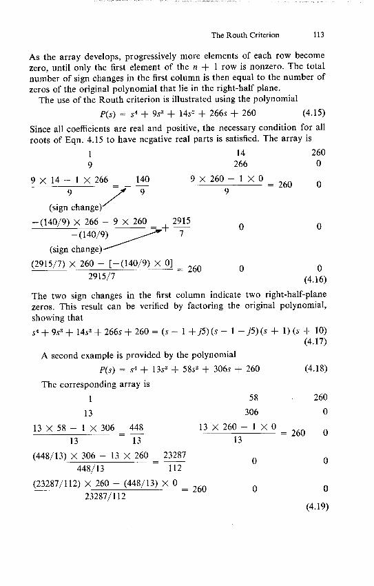
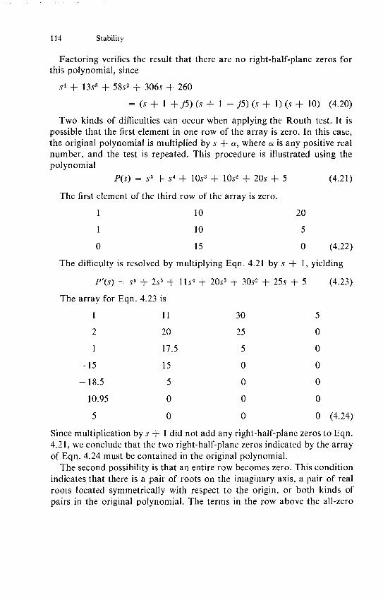
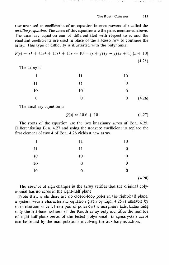
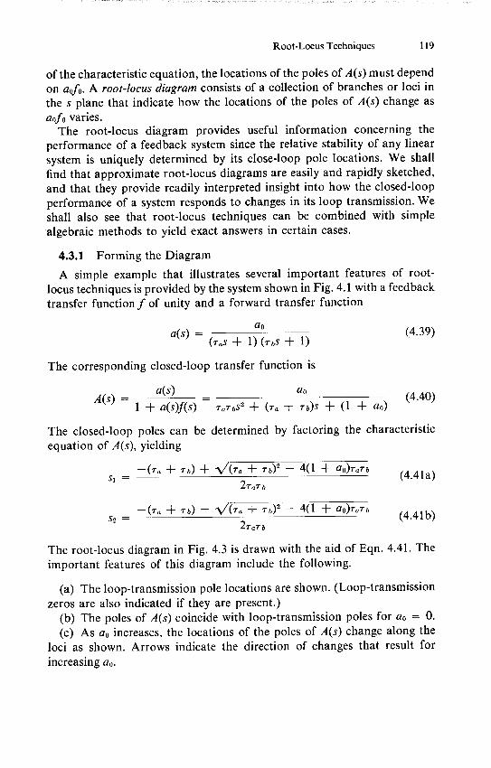
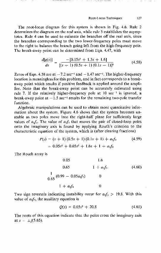
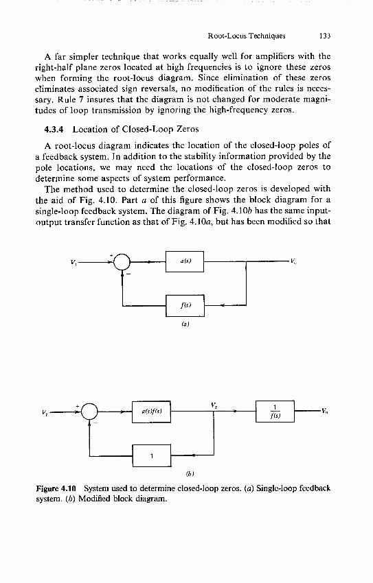
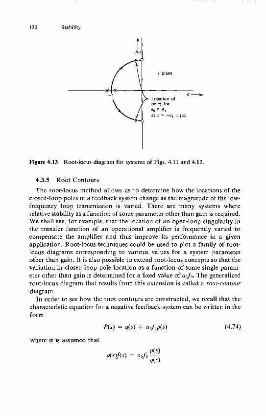
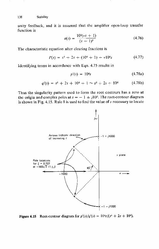

I
s plane
a DO
(a)
Value for s = jO Value for s = jOshy
-180 +18( Z [a(jo)f(j) 1 shy
af plane
(b)
Figure 420 Nyquist test for a(s)f(s) = ao(s - 1) (a) s-plane plot (b) af-plane plot (c) af-plane plot (polar coordinates)
146
147 Stability Based on Frequency Response
(C)
Figure 420-Continued
1 If the magnitude of af is 1 at only one frequency the system is stable if the angle of af is between + 1800 and - 1800 at the unity-gain frequency
2 If the angle of af passes through +180 or - 1800 at only one freshyquency the system is stable if the magnitude of af is less than 1 at this frequency
Information concerning the relative stability of a feedback system can also be determined from a Bode plot for the following reason The values of s for which af = - 1 are the closed-loop pole locations of a feedback system The Nyquist test exploits this relationship in order to determine the absolute stability of a system If the system is stable but a pair of - ls of afoccur for values of s close to the imaginary axis the system must have a pair of closed-loop poles with a small damping ratio
The quantities shown in Fig 421 provide a useful estimation of the proximity of - ls of af to the imaginary axis and thus indicate relative stability The phase margin is the difference between the angle of af and - 1800 at the frequency where the magnitude of af is 1 A phase margin of 00 indicates closed-loop poles on the imaignary axis and therefore the phase margin is a measure of the additional negative phase shift at the unity-magnitude frequency that will cause instability Similarly the gain margin is the amount of gain increase required to make the magnitude of af unity at the frequency where the angle of af is - 1800 and represents the
148 Stability
la w)f(j o) I
1shy
aaqL~f(jco)
0 shy -ushy
marain G mase
-1800
wc unity-gain frequency
Figure 421 Loop-transmission quantities
amount of increase in aofo required to cause instability The frequency at which the magnitude of af is unity is called the unity-gainfrequency or the crossoverfrequency This parameter characterizes the relative frequency reshysponse or speed of the time response of the system
A particularly valuable feature of analysis based on the loop-transmission characteristics of a system is that the gain margin and the phase margin quantities that are quickly and easily determined using Bode techniques give surprisingly good indications of the relative stability of a feedback system It is generally found that gain margins of three or more combined with phase margins between 30 and 60 result in desirable trade-offs beshytween bandwidth or rise time and relative stability The smaller values for gain and phase margin correspond to lower relative stability and are avoided
149 Stability Based on Frequency Response
if small overshoot in response to a step or small frequency-response peaking is necessary or if there is the possibility of severe changes in parameter values
The closed-loop bandwidth and rise time are almost directly related to the unity-gain frequency for systems with equal gain and phase margins Thus any changes that increase the unity-gain frequency while maintaining constant values for gain and phase margins tend to increase closed-loop bandwidth and decrease closed-loop rise time
Certain relationships between these three quantities and the correspondshying closed-loop performance are given in the following section Prior to presenting these relationships it is emphasized that the simplicity and excellence of results associated with frequency-response analysis makes this method a frequently used one particularly during the initial design phase Once a tentative design based on these concepts is determined more deshytailed information such as the exact location of closed-loop singularities or the transient response of the system may be investigated frequently with the aid of machine computation
443 Closed-Loop Performance in Terms of Loop-Transmission Parameters
The quantity a(j)f(jw) can generally be quickly and accurately obtained in Bode-plot form The effects of system-parameter changes on the loop transmission are also easily determined Thus approximate relationships between the loop transmission and closed-loop performance provide a useful and powerful basis for feedback-system design
The input-output relationship for a system of the type illustrated in Fig 41Oa is
V0(s) _ a(s)A(s= a(s) (484)
Vi(s) 1 + a(s)f(s)
If the system is stable the closed-loop transfer function of the system can be approximated for limiting values of loop transmission as
A(jo) ~- a(jw)f(jw) gtgt 1 (485a)
A(jw) a(jw) Ia(jw)f(je) lt 1 (485b)
One objective in the design of feedback systems is to insure that the approximation of Eqn 485a is valid at all frequencies of interest so that the system closed-loop gain is controlled by the feedback element The approximation of Eqn 485b is relatively unimportant since the system is
150 Stability
effective operating without feedback in this case While we normally do not expect to have the system provide precisely controlled closed-loop gain at frequencies where the magnitude of the loop transmission is close to one the discussion of Section 442 shows that the relative stability of a system is largely determined by its performance in this frequency range
The Nichols chart shown in Fig 422 provides a convenient method of evaluating the closed-loop gain of a feedback system from its loop trans-
G I 0999
-0998
0995
099
098
095
09
08
05
- 35991+G
-3598
-359
--3580
-355011 UII-
-350
-340
1001
1002
1005
101
102
105
12
15 2 3
G 01Gshy
1+G
-02-
-05
-1 V1
-2shy
-5Iy -10 IIII
-20-
103
1052
- 102
3
GI
10
1012
1
( I in-12
32
-52
-3600 -3300 -3000 -2700 -2400 -2100 -180 -1500 -1200 -900 -600 -300 00
Figure 422 Nichols chart
151 Stability Based on Frequency Response
mission and is particularly valuable when neither of the limiting approxishymations of Eqn 485 is valid This chart relates G(1 + G) to G where G is any complex number In order to use the chart the value of G is located on the rectangular gain-phase coordinates The angle and magnitude of G(1 + G) are than read directly from the curved coordinates that intersect the value of G selected
The gain-phase coordinates shown in Fig 422 cover the complete 00 to -360 range in angle and a ratio of 106 in magnitude This magnitude range is unnecessary since the approximations of Eqn 485 are usually valid when the loop-transmission magnitude exceeds 10 or is less than 01 Similarly the range of angles of greatest interest is that which surrounds the -1800 value and which includes anticipated phase margins The Nichols chart shown in Fig 423 is expanded to provide greater resolution in the region where it will normally be used
One effective way to view the Nichols chart is as a three-dimensional surface with the height of the surface proportional to the magnitude of the closed-loop transfer function corresponding to the loop-transmission parameters that define the point of interest This visualization shows a mountain (with a peak of infinite height) where the loop transmission is +1
The Nichols chart can be used directly for any unity-gain feedback sysshytem The transformation indicated in Fig 410b shows that the chart can be used for arbitrary single-loop systems by observing that
A(jw) = a(jw) [ a(jo)f(j I) ~1 ] (486)1 + a(jo)f(jo) 1 + a(jw)f(jj)f(jo)_
The closed-loop frequency response is determined by multiplying the factor a(jw)f(j)[1 + a(jw)f(jo)] obtained via the Nichols chart by If(j) using Bode techniques
One quantity of interest for feedback systems with frequency-independent feedback paths is the peak magnitude M equal to the ratio of the maxishymum magnitude of A(jw) to its low-frequency magnitude (see Section 35) A large value for M indicates a relatively less stable system since it shows that there is some frequency for which the characteristic equation approaches zero and thus that there is a pair of closed-loop poles near the imaginary axis at approximately the peaking frequency Feedback amplifiers are frequently designed to have Ms between 11 and 15 Lower values for MP imply greater relative stability while higher values indicate that stability has been compromised in order to obtain a larger low-frequency loop transmission and a higher crossover frequency
The value of M for a particular system can be easily determined from the Nichols chart Furthermore the chart can be used to evaluate the
100
70
50
-shy 2o - 30
-105 -3 -- 20
098 __14
11 -5 - 10
-115 -71
-10 095 012
13 5
14 -15o 09 |G 1
-15-20 085 -3 17
2 -30 08 -- 2
43 -40 071 025
6 1shy
06
-60shy-- 05 - 07
p3-- 05
Oo 03 - 03
-- $0O 024G-o o oo -02
014
-- 190 -180-170-1600-150 -140 -130 -120 -1100-100 -90 -80 -70 -600
4 G shy
Figure 423 Expanded Nichols chart
152
153 Stability Based on Frequency Response
effects of variations in loop transmission on M One frequently used manipulation determines the relationship between M and aofo for a system with fixed loop-transmission singularities The quantity a(jW)f(jW)aofo is first plotted on gain-phase coordinates using the same scale as the Nichols chart If this plot is made on tracing paper it can be aligned with the Nichols chart and slid up or down to illustrate the effects of different values of aofo The closed-loop transfer function is obtained directly from the Nichols chart by evaluating A(jw) at various frequencies while the highest magnitude curve of the Nichols chart touched by a(jw)f(jw) for a particular value of aofo indicates the corresponding M
Figure 424 shows this construction for a system with f = 1 and
a(s) = a(487)(s + 1) (01s + 1)
The values of ao for the three loop transmissions are 85 22 and 50 The corresponding Ms are 1 14 and 2 respectively
While the Nichols chart is normally used to determine the closed-loop function from the loop transmission it is possible to use it to go the other way that is to determine a(j)f(jo) from A(jw) This transformation is
occasionally useful for the analysis of systems for which only closed-loop measurements are practical The transformation yields good results when the magnitude of a(j)f(jw) is close to one Furthermorethe approximation of Eqn 485b shows tha A(jw) - a(jw) when the magnitude of the loop transmission is small However Eqn 485a indicates that A(jw) is essenshytially independent of the loop transmission when the loop-transmission magnitude is large Examination of the Nichols chart confirms this result since it shows that very small changes in the closed-loop magnitude or angle translate to very large changes in the loop transmission for large loop-transmission magnitudes Thus even small errors in the measurement of A(jw) preclude estimation of large values for a(jo)f(jw) with any accuracy
The relative stability of a feedback system and many other important characteristics of its closed-loop response are largely determined by the behavior of its loop transmission at frequencies where the magnitude of this quantity is close to unity The approximations presented below relate closed-loop quantities defined in Section 35 to the loop-transmission properties defined in Section 442 These approximations are useful for
predicting closed-loop response comparing the performance of various systems and estimating the effects of changes in loop transmission on
closed-loop performance The assumptions used in Section 35 in particular that f is one at all
-14 - 1 01 o G |I
-15 =10 201
= 2085 --3
-17 08shy-2 N -2 25 = 5 -30 -3 =10 07 _4
46 _40 5 0 06 -
05- 0
C = 10 S=20 -O -
03shyS=50 0-03
o Go O02shyo Oo -02
o = 50 014
1 01 -190-70 -15 -140-130 -- 120 -- 11Cf -100 -90 -- 80 -706
ao =50 ao =22 ao = 85 G
Figure 424 Determination of closed-loop transfer function for a(s) = aol[(s + 1)(O1s + 1)]f= 1
154
155 Stability Based on Frequency Response
frequencies that ao is large and that the lowest frequency singularity of a(s) is a pole are assumed here Under these conditions
M ~ sin 1kmn (488)
where $mis the phase margin The considerations that lead to this approxishymation are illustrated in Fig 425 This figure shows several closed-loopshymagnitude curves in the vicinity of M = 14 and assumes that the system phase margin is 45 Since the point G = 1 4 G = -135 must exist
10
Mp 135
G 12
13 Mp = 13
14
15 3
17 shy
MP= 15
-1
IG |
Gain margin
223 Gain - 03 margin
-27
-1930 -180
4GG
1_ -135
l
101 -90
Figure 425 M for several systems with 450 of phase margin
156 Stability
for a system with a 450 phase margin there is no possible way that M can be less than approximately 13 and the loop-transmission gain-phase curve must be quite specifically constrained for M just to equal this value If it is assumed that the magnitude and angle of G are linearly related the linear constructions included in Fig 425 show that M cannot exceed approximately 15 unless the gain margin is very small Well-behaved sysshytems are actually most likely to have a gain-phase curve that provides an extended region of approximate tangency to the M = 14 curve for a phase margin of 450 Similar arguments hold for other values of phase margin and the approximation of Eqn 488 represents a good fit to the relationship between phase margin and corresponding M
Two other approximations relate the system transient response to its crossover frequency we
06 22 -- lt tr lt - (489) wc (Jc
The shorter values of rise time correspond to lower values of phase margin
4 t gt - (490)
COc
The limit is approached only for systems with large phase margins We shall see that the open-loop transfer function of many operational
amplifiers includes one pole at low frequencies and a second pole in the vicinity of the unity-gain frequency of the amplifier If the system dynamics are dominated by these two poles the damping ratio and natural frequency of a second-order system that approximates the actual closed-loop system can be obtained from Bode-plot parameters of a system with a frequency-independent feedback path using the curves shown in Fig 426a The curves shown in Fig 426b relate peak overshoot and M for a second-order system to damping ratio and are derived using Eqns 358 and 362 While the relationships of Fig 426a are strictly valid only for a system with two widely spaced poles in its loop transmission they provide an accurate approximashytion providing two conditions are satisfied
1 The system loop-transmission magnitude falls off as l1w at frequencies between one decade below crossover and the next higher frequency singushylarity
2 Additional negative phase shift is provided in the vicinity of the crossshyover frequency by other components of the loop transmission
The value of these curves is that they provide a way to determine an approximating second-order system from either phase margin M or peak
0
157 Stability Based on Frequency Response
10
08
s 0606shyE
~0 04 0
02 shy
0 0
02
175 shy
cc 1753 3
125 shy
10 01 20 40 60 80 100
Phase margin
Figure 426a Closed-loop quantities from loop-transmission parameters for system with two widely spaced poles Damping ratio and natural frequency as a function of phase margin and crossover frequency
overshoot of a complex system The validity of this approach stems from the fact that most systems must be dominated by one or two poles in the vicinity of the crossover frequency in order to yield acceptable performance Examples illustrating the use of these approximations are included in later sections We shall see that transient responses based on the approximation are virtually indistinguishable from those of the actual system in many cases of interest
158 Stability
18 shy
16 shy
O 14 shy
12 shy
10
18 shy
16 shy
14
12 shy
10 0 02 04 06 08 10
Damping ratio
Figure 426b Po and M versus damping ratio for second-order system
The first significant error coefficient for a system with unity feedback can also be determined directly from its Bode plot If the loop transmission includes a wide range of frequencies below the crossover frequency where its magnitude is equal to kwn the error coefficients eo through e- are negligible and e equals 1k
PROBLEMS P41 Find the number of right-half-plane zeros of the polynomial
P(s) = s1 + s 4 + 3s + 4s2 + s + 2
Problems 159
P42 A phase-shift oscillator is constructed with a loop transmission
ao--=L(s) 1)4(r-S +
Use the Routh condition to determine the value of ao that places a pair of closed-loop poles on the imaginary axis Also determine the location of the poles Use this information to factor the characteristic equation of the system thus finding the location of all four closed-loop poles for the critical value of ao
P43 Describe how the Routh test can be modified to determine the real parts
of all singularities in a polynomial Also explain why this modification is usually of little value as a computational aid to factoring the polynomial
P44 Prove the root-locus construction rule that establishes the angle and
intersection of branch asymptotes with the real axis
P45 Sketch root-locus diagrams for the loop-transmission singularity pattern
shown in Fig 427 Evaluate part c for moderate values of aofo and part d for both moderate and very large values of aofo
P46 Consider two systems both with f = 1 One of these systems has a
forward-path transfer function
a(s) = ao(O5s + 1) (s + 1) (001s + 1) (051s + 1)
while the second system has
ao(O51s + 1)a(S) = (s + 1) (001s + 1) (05s + 1)
Common sense dictates that the closed-loop transfer functions of these
systems should be very nearly identical and furthermore that both should be similar to a system with
a(s) =a (s + 1) (001s + 1)
[The closely spaced pole-zero doublets in a(s) and a(s) should effectively
cancel out] Use root-locus diagrams to show that the closed-loop responses are in fact similar
160 Stability
jL
s plane
a bshy-4 -3 -2 -1
(a)
jo j1
s plane
-2 -1
j1
(b)
Figure 427 Loop-transmission singularity patterns
P47 An operational amplifier has an open-loop transfer function
106a(s) = (0ls + 1) (10-6s + 1)2
This amplifier is combined with two resistors in a noninverting-amplifier configuration Neglecting loading determine the value of closed-loop gain that results when the damping ratio of the complex closed-loop pole pair is 05
P48 An operational amplifier has an open-loop transfer function
105 a(s) = 10 +
(rS + 1) (10-6S + 1)
The quantity T can be adjusted by changing the amplifier compensation
t
s plane
-x -1000
( 5 X -3
X -2
x -1
(c)
I
s plane
-0- 0 X )x X
-2000 -1000 -3 -2 -1
(d)
x t
s plane
-2 -1 a N
--j1
(e)
Figure 427-Continued
161
162 Stability
Use root-contour techniques to determine a value of r that results in a closed-loop damping ratio of 0707 when the amplifier is connected as a unity-gain inverter
P49 A feedback system that includes a time delay has a loop transmission
aoe-0013L~)L(s) = a- 0 l(s + 1)
Use the Nyquist test to determine the maximum value of ao for stable operation What value of ao should be selected to limit M to a factor of 14 (You may assume that the feedback path of the system is frequency independent)
P410 We have been investigating the stability of feedback systems that are
generally low pass in nature since the transfer functions of most operashytional-amplifier connections fall in this category However stability probshylems also arise in high-pass systems For example a-c coupled feedback amplifiers designed for use at audio frequencies sometimes display a low-frequency instability called motor-boating Use the Nyquist test to demonstrate the possibility of this type of instability for an amplifier with a loop transmission
L(s) - aosa (s + 1) (0ls + 1)2
Also show the potentially unstable behavior using root-locus methods For what range of values of ao is the amplifier stable
P411 Develop a modification of the Nyquist test that enables you to determine
if a feedback system has any closed-loop poles with a damping ratio of less than 0707 Illustrate your test by forming the modified Nyquist diagram for a system with a(s) = ao(s + 1)
2 f(s) = 1 For what value of ao does the damping ratio of the closed-loop pole pair equal 0707 Verify your answer by factoring the characteristic equation for this value of ao
P412 The open-loop transfer function of an operational amplifier is
1050a(s) = (0s + 1) (10-s + 1)2
Determine the gain margin phase margin crossover frequency and M for this amplifier when used in a feedback connection withf = 1 Also find
Problems 163
the value off that results in an M of 11 What are the values of phase and gain margin and crossover frequency with this value forf
P413 A feedback system is constructed with
a(s) = 106(0Ols + 1)2 (s + 1)3
and an adjustable frequency-independent value forfAsf is increased from zero it is observed that the system is stable for very small values off then becomes unstable and eventually returns to stable behavior for sufficiently high values of f Explain this performance using Nyquist and root-locus analysis Use the Routh criterion to determine the two borderline values for f
P414 An operational amplifier with a frequency-independent feedback path
exhibits 40 overshoot and 10 to 90 rise time of 05 ps in response to a
step input Estimate the phase margin and crossover frequency of the feedshyback connection assuming that its performance is dominated by two widely separated loop-transmission poles
P415 Consider a feedback system with
=a(s) a 0
s[(s22) + s + 1]
and f(s) = 1 Show that by appropriate choice of ao the closed-loop poles of the system
can be placed in a third-order Butterworth pattern Find the crossover frequency and the phase margin of the loop transmission when ao is selected for the closed-loop Butterworth response Use these quantities in conjuncshytion with Fig 426 to find the damping ratio and natural frequency of a
second-order system that can be used to approximate the transient response of the third-order Butterworth filter Compare the peak overshoot and rise
time of the approximating system in response to a step with those of the
Butterworth response (Fig 310) Note that even though this system is conshy
siderably different from that used to develop Fig 426 the approximation predicts time-domain parameters with fair accuracy
1V
MIT OpenCourseWarehttpocwmitedu
RES6-010 Electronic Feedback SystemsSpring 2013
For information about citing these materials or our Terms of Use visit httpocwmiteduterms
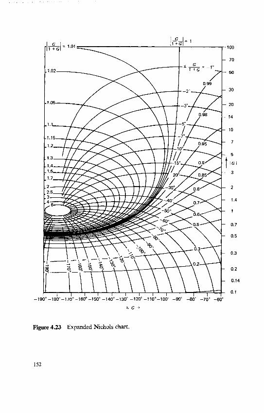
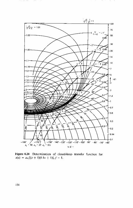
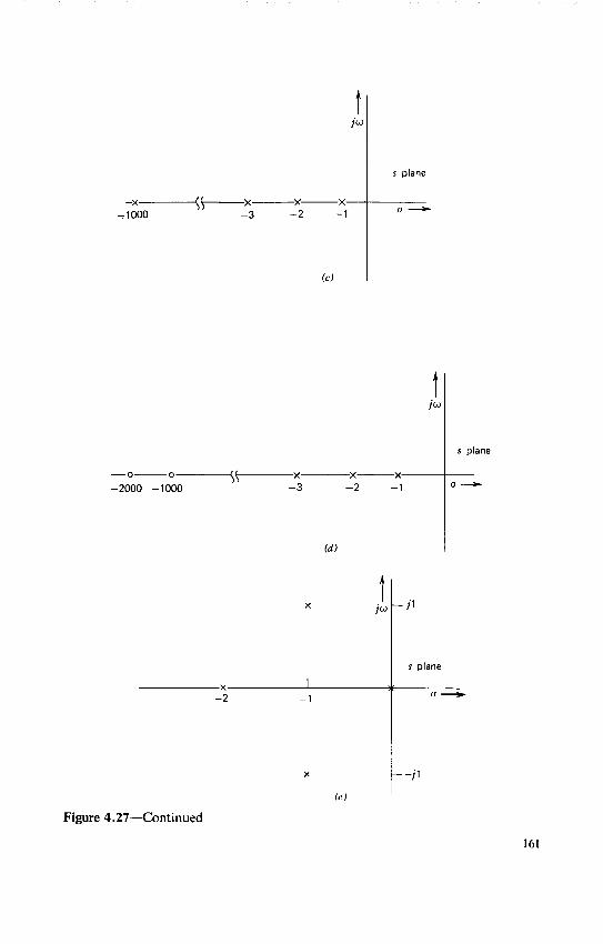

1V
MIT OpenCourseWarehttpocwmitedu
RES6-010 Electronic Feedback SystemsSpring 2013
For information about citing these materials or our Terms of Use visit httpocwmiteduterms

MIT OpenCourseWarehttpocwmitedu
RES6-010 Electronic Feedback SystemsSpring 2013
For information about citing these materials or our Terms of Use visit httpocwmiteduterms


![8. [BIC 2015] Spotlight - TOP 10 BIC 2015](https://img.pdfslide.net/doc/110x75/587c3d6b1a28ab5a1d8b57e5/8-bic-2015-spotlight-top-10-bic-2015.jpg)


![10. [BIC 2015] FABU - TOP 10 BIC 2015](https://img.pdfslide.net/doc/110x75/587c3d801a28ab5a1d8b5841/10-bic-2015-fabu-top-10-bic-2015.jpg)