Embed Size (px)
Citation preview
CHAPTER VI
NONLINEAR SYSTEMS
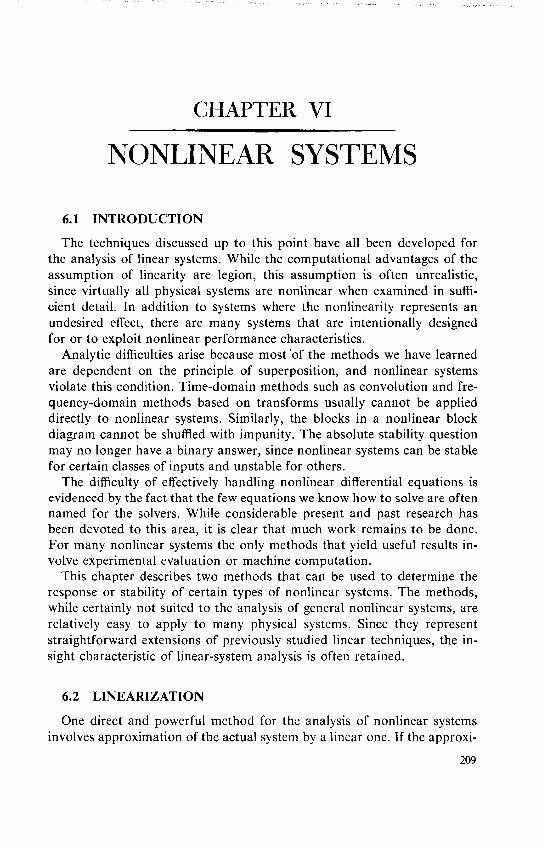
6.1 INTRODUCTION
The techniques discussed up to this point have all been developed for the analysis of linear systems. While the computational advantages of the assumption of linearity are legion, this assumption is often unrealistic, since virtually all physical systems are nonlinear when examined in sufficient detail. In addition to systems where the nonlinearity represents an undesired effect, there are many systems that are intentionally designed for or to exploit nonlinear performance characteristics.
Analytic difficulties arise because most'of the methods we have learned are dependent on the principle of superposition, and nonlinear systems violate this condition. Time-domain methods such as convolution and frequency-domain methods based on transforms usually cannot be applied directly to nonlinear systems. Similarly, the blocks in a nonlinear block diagram cannot be shuffled with impunity. The absolute stability question may no longer have a binary answer, since nonlinear systems can be stable for certain classes of inputs and unstable for others.
The difficulty of effectively handling nonlinear differential equations is evidenced by the fact that the few equations we know how to solve are often named for the solvers. While considerable present and past research has been devoted to this area, it is clear that much work remains to be done. For many nonlinear systems the only methods that yield useful results involve experimental evaluation or machine computation.
This chapter describes two methods that can be used to determine the response or stability of certain types of nonlinear systems. The methods, while certainly not suited to the analysis of general nonlinear systems, are relatively easy to apply to many physical systems. Since they represent straightforward extensions of previously studied linear techniques, the insight characteristic of linear-system analysis is often retained.
6.2 LINEARIZATION
One direct and powerful method for the analysis of nonlinear systems involves approximation of the actual system by a linear one. If the approxi
209
210 Nonlinear Systems
mating system is correctly chosen, it accurately predicts the behavior of the actual system over some restricted range of signal levels.
This technique of linearization based on a tangent approximation to a nonlinear relationship is familiar to electrical engineers, since it is used to model many electronic devices. For example, the bipolar transistor is a highly nonlinear element. In order to develop a linear-region model such as the hybrid-pi model to predict the circuit behavior of this device, the relationships between base-to-emitter voltage and collector and base current are linearized. Similarly, if the dynamic performance of the transistor is of interest, linearized capacitances that relate incremental changes in stored charge to incremental changes in terminal voltages are included in the model.
6.2.1 The Approximating Function
The tangent approximation is based on the use of a Taylor's series estimation of the function of interest. In general, it is assumed that the output variable of an element is a function of N input variables
vo = F(v 11, v12 , . . . , VIN) (6.1)
The output variable is expressed for small variation vi,, Vi 2 , ... , viN about input-variable operating points V11, Vr 2 , . . . , VIN by noting that
VO = Vo + v. = F(V1 1 , V 1 2, VIN)
N VO + I Vii
(=VIj Vn1,V 12,...,VIN
1 N g2 + E vikVil --. + (6.2)
aVka V11, V2!k,= I VI1 1 2,..VIN
(Recall that the variable and subscript notation used indicates that vo is a total variable, Vo is its operating-point value, and v0 its incremental component.)
The expansion of Eqn. 6.2 is valid at any operating point where the derivatives exist.
Since the various derivatives are assumed bounded, the function can be adequately approximated by the first-order terms over some restricted range of inputs. Thus
VO + vo - F(V1 1, V1 2, . . . , VIN) i (.3 j-i a VIj VI, V12, VIN
211 Linearization
Vi 2 1 -'I 3I1IaV2 PbVO
Vi N--3-1 W I N V I, , VI2 --.-VIN
N V
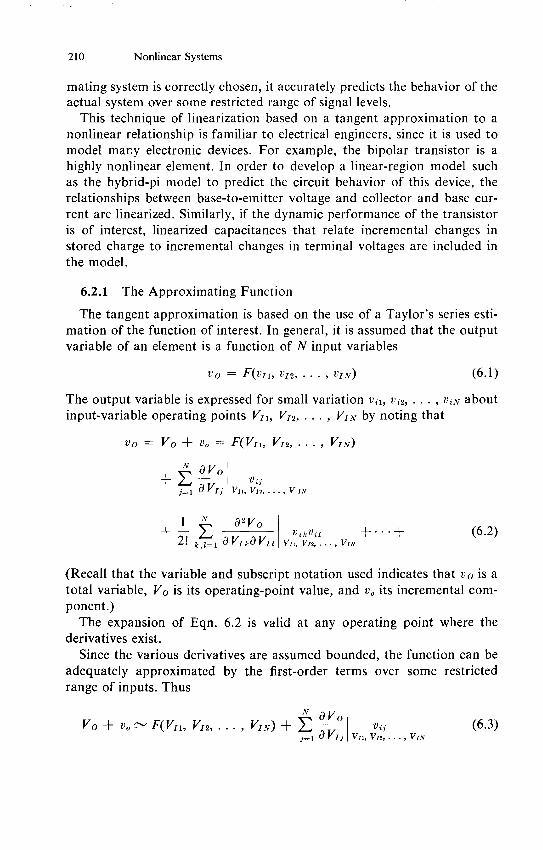
Figure 6.1 Linearized block diagram.
The constant terms in Eqn. 6.3 are substracted out, leaving
N~VO vij (6.4) j-i 0 V1 I V11, V12,- VIN
Equation 6.4 can be used to develop linear-system equations that relate incremental rather than total variables and that approximate the incremental behavior of the actual system over some restricted range of opera
tion. A block diagram of the relationships implied by Eqn. 6.4 is shown in
Fig. 6.1.
6.2.2 Analysis of an Analog Divider
Certain types of signal-processing operations require that the ratio of
two analog variables be determined, and this function can be performed
by a divider. Division is frequently accomplished by applying feedback around an analog multiplier, and several commercially available multi
pliers can be converted to dividers by making appropriate jumpered con
nections to the output amplifier included in these units. A possible divider
connection of this type is shown in Fig. 6.2a.
The multiplier scale factor shown in this figure is commonly used since
it provides a full-scale output of 10 volts for two 10-volt input signals. It

R
VA
R
VD
Multiplier
V vB VC D 10
VB
VCc
Va
T
a
N
+ 1-a(s)
+.
(a)
vv
10
VB
10O 1-0
Figure 6.2
V (b)
Analog divider. (a) Circuit. (b) Linearized block diagram.
212

213 Linearization
is assumed that the multiplying element itself has no dynamics and thus the speed of response of the system is determined by the operational amplifier.
The ideal relationship between input and output variables can easily be determined using the virtual-ground method. If the current at the inverting input of the amplifier is small and if the magnitude of the loop transmission is high enough so that the voltage at this terminal is negligible, the circuit
relationships are
VA+ VD 0 (6.5)
and
VD VBVC
=-(6*6)10
VBVO
10
Solving Eqns. 6.5 and 6.6 for vo in terms of VA and VB yields
o = OVA (6.7) VB
System dynamics are determined by linearizing the multiplying-element characteristics. Applying Eqn. 6.3 to the variables of Eqn. 6.6 shows that
VC 68VD+Vd B VBVc VCVb 10 10 10
The incremental portion of this equation is
VBVc VCVb vd - + (6.9)
10 10
This relationship combined with other circuit constraints (assuming the
operational amplifier has infinite input impedance and zero output im
pedance) is used to develop the incremental block diagram shown in Fig. 6.2b.
The incremental dependence of V on V,, assuming that VB is constant,
is V0(s) _ - a(s)/2 (6.10) Va(s) 1 + VBa(s)120
If the operational-amplifier transfer function is approximately single pole
so that
a(s) ao (6.11) rS + 1
214 Nonlinear Systems
and ao is very large, Eqn. 6.10 reduces to
V/0(s) -10/'VBV"S) - 0' (6.12)V0(s) (20r Vaao)s + I
Several features are evident from this transfer function. First, if VB is negative, the system is unstable. Second, the incremental step response of the system is first order, with a time constant of 2
0r VBao seconds. These features indicate two of the many ways that nonlinearities can affect the performance of a system. The stability of the circuit depends on an input-signal level. Furthermore, if VB is positive, the transient response of the circuit becomes faster with increasing VB, since the loop transmission depends on the value of this input.
6.2.3 A Magnetic-Suspension System
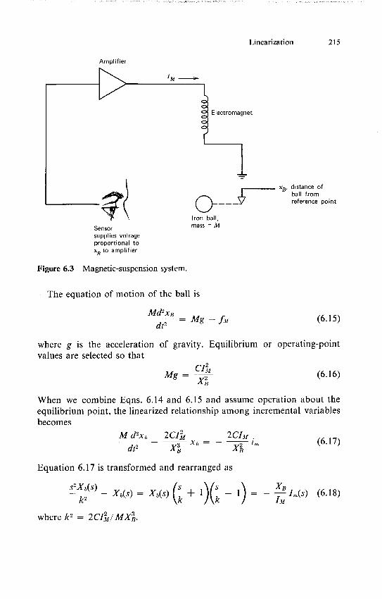
An electromechanical system that provides a second example of linearized analysis is illustrated in Fig. 6.3. The purpose of the system is to suspend an iron ball in the field of an electromagnet. Only vertical motion of the ball is considered.
In order to suspend the ball it is necessary to cancel the downward gravitational force on the ball with an upward force produced by the magnet. It is clear that stabilization with constant current is impossible, since while a value of XB for which there is no net force on the ball exists, a small deviation from this position changes the magnetic force in such a way as to accelerate the ball further from equilibrium. This effect can be cancelled by appropriately controlling the magnet current as a function of measured ball position.
For certain geometries and with appropriate choice of the reference position for XB, the magnetic force fM exerted on the ball in an upward direction is
f = Ci2 fl 2 (6.13)
XB
where C is a constant. Assuming incremental changes Xb and im about operating-point values
XB and IM, respectively,
CI2CIMfM=FMfm -- 2 2 m -CI3 Xb
B Bi
+ higher-order terms (6.14)
215 Linearization
Amplifier
Electromagnet
xB, distance of ball from reference point
Iron ball, mass = MSensor
supplies voltage proportional to xB to amplifier
Figure 6.3 Magnetic-suspension system.
The equation of motion of the ball is
Md'xB (6.15)
dt2 - fi= Mg
where g is the acceleration of gravity. Equilibrium or operating-point values are selected so that
Mg - (6.16) X'B
When we combine Eqns. 6.14 and 6.15 and assume operation about the equilibrium point, the linearized relationship among incremental variables becomes
M d2xb 2CI 2CI . (6.17)
dt2 - X3 x=- - XB .
Equation 6.17 is transformed and rearranged as
s2 Xb(s) s + s XB -- 1 1 - IM Im(s) (6.18)
2 - Xb(s) = Xb(s)
where k2 = 2C4m/ MXB.
216 Nonlinear Systems
1, (s)
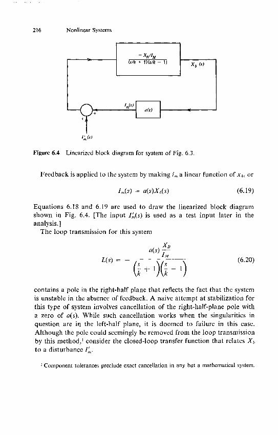
Figure 6.4 Linearized block diagram for system of Fig. 6.3.
Feedback is applied to the system by making im a linear function of Xb, or
Im(s) = a(s)Xb(s) (6.19)
Equations 6.18 and 6.19 are used to draw the linearized block diagram shown in Fig. 6.4. [The input If,(s) is used as a test input later in the analysis.]
The loop transmission for this system
a(s) XB
L(s) = - (6.20)
+1) - )
contains a pole in the right-half plane that reflects the fact that the system
is unstable in the absence of feedback. A naive attempt at stabilization for
this type of system involves cancellation of the right-half-plane pole with
a zero of a(s). While such cancellation works when the singularities in
question are in the left-half plane, it is doomed to failure in this case.
Although the pole could seemingly be removed from the loop transmission
by this method,' consider the closed-loop transfer function that relates Xb to a disturbance Ij.
I Component tolerances preclude exact cancellation in any but a mathematical system.

217 Describing Functions
If a(s) is selected as a'(s)(s/k - 1), this transfer function is
- XB Ji
Xb(s) (s/k + 1)(s/k - 1) (6.21)
I'(s) a'(s) XB IM I+s/k + I
Equation 6.21 contains a right-half-plane pole implying exponentially growing responses for Xb even though this growth is not observed as a change in i,.
A satisfactory method for compensating the system can be determined by considering the root-locus diagrams shown in Fig. 6.5. Figure 6.5a is the diagram for frequency-independent feedback with a(s) = ao. As ao is increased, the two poles come together and branch out along the imaginary axis. This diagram shows that it is possible to remove the closed-loop pole from the right-half plane if ao is appropriately chosen. However, the poles cannot be moved into the left-half plane, and thus the system exhibits undampened oscillatory responses. The system can be stabilized by including a lead transfer function in a(s). It is possible to move all closed-loop poles to the left-half plane for any lead-network parameters coupled with a sufficiently high value of ao. Figure 6.5b illustrates the root trajectories for one possible choice of lead-network singularities.
6.3 DESCRIBING FUNCTIONS
Describing functions provide a method for the analysis of nonlinear systems that is closely related to the linear-system techniques involving Bode or gain-phase plots. It is possible to use this type of analysis to determine if limit cycles (constant-amplitude periodic oscillations) are possible for a given system. It is also possible to use describing functions to predict the response of certain nonlinear systems to purely sinusoidal excitation, although this topic is not covered here.2 Unfortunately, since the frequency response and transient response of nonlinear systems are not directly related, the determination of transient response is not possible via describing functions.
6.3.1 The Derivation of the Describing Function
A describing function describes the behavior of a nonlinear element for purely sinusoidal excitation. Thus the input signal applied to the nonlinear
2 G. J. Thaler and M. P. Pastel, Analysis and Design of Nonlinear Feedback Control
Systems, McGraw-Hill, New York, 1962.

218 Nonlinear Systems
t s plane
s = -k I s = k a -
(a)
Singularities s planefrom lead
network
s=k a
(b)
Figure 6.5 Root-locus diagrams for magnetic-suspension system. (a) Uncompensated. (b) With lead compensation.
element to determine its describing function is
vr = E sin wt (6.22)
If the nonlinearity does not rectify the input (produce a d-c output) and does not introduce subharmonics, the output of the nonlinear element can be expanded in a Fourier series of the form
vo = A1(E, w) cos wt + B 1(E, co) sin wt + A 2(E, o) cos 2 wt
+ B2(E, o) sin 2wt + - + (6.23)

219 Describing Functions
The describing function for the nonlinear element is defined as
IVA2(E, ) + B2(E, t) A1(E, c)GD(E, ) 4 tan-B 1 (E, ) (6.24)
The describing-function characterization of a nonlinear element parallels the transfer-function characterization of a linear element. If the transfer function of a linear element is evaluated for s = jo, the magnitude of resulting function of a complex variable is the ratio of the amplitudes of the output and input signals when the element is excited with a sinusoid at a frequency co. Similarly, the angle of the function is the phase angle between the output and input signals under sinusoidal steady-state conditions. For linear elements these quantities must be independent of the amplitude of excitation.
The describing function indicates the relative amplitude and phase angle of thefundamentalcomponent of the output of a nonlinear element when the element is excited with a sinusoid. In contrast to the case with linear elements, these quantities can be dependent on the amplitude as well as the frequency of the excitation.
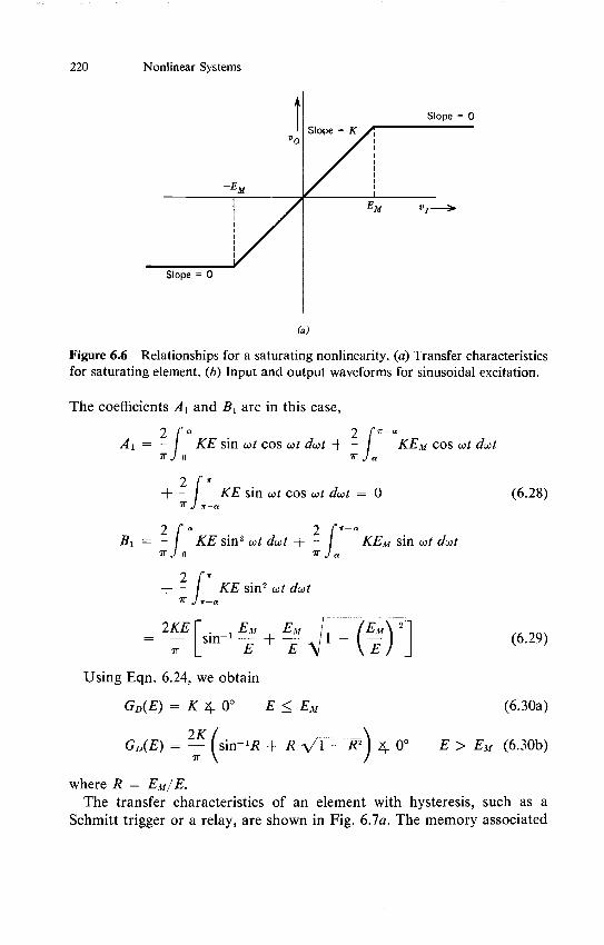
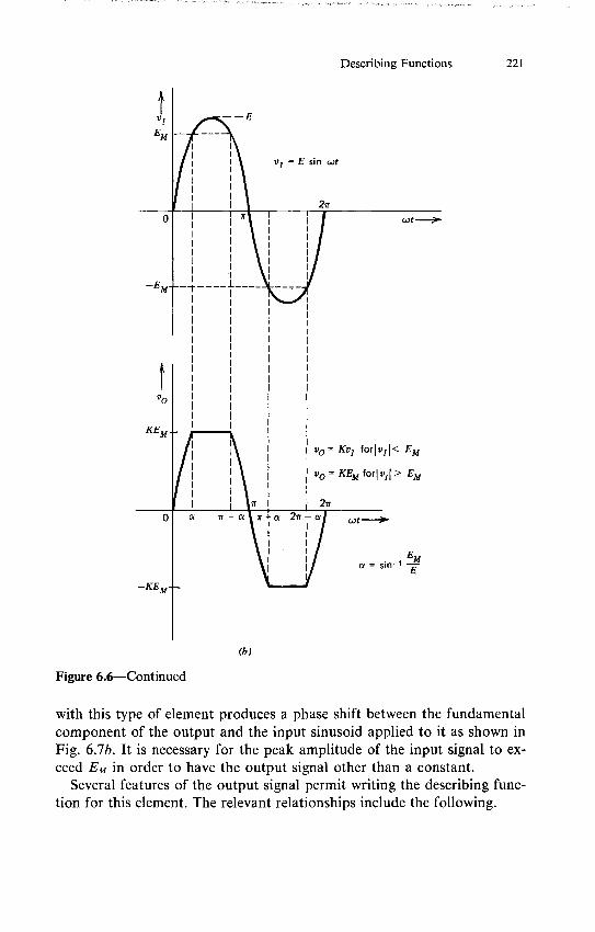
Two examples illustrate the derivation of the describing function for nonlinear elements. Figure 6.6 shows the transfer characteristics of a saturating nonlinearity together with input and output waveforms for sinusoidal excitation. Since the transfer characteristics for this element are not dependent on the dynamics of the input signal, it is clear that the describing function must be frequency independent.
If the input amplitude E is less than EM,
0 = Kyr (6.25)
In this case,
GD = K 4 0 E < E (6.26)
For E > E, the output signal over the interval 0< at< r is
vo = K 0 < wt < a or r - a < wt < r (6.27a)
vo = KEu1 a < wt < r - a (6.27b)
where
a = sin-1 E
220 Nonlinear Systems
Slope = 0 I
V 0
-EM
EM vi;0
(a)
Figure 6.6 Relationships for a saturating nonlinearity. (a) Transfer characteristics for saturating element. (b) Input and output waveforms for sinusoidal excitation.
The coefficients A1 and B 1 are in this case,
A1 - KE sin wt coswt dt + - KE. cos wt dt
+ J KE sin wt cos wt dwt = 0 (6.28)
2r ra2
B1 = fKE sins cot dcot + - KE sin cot dwt
2 i + - KE sin 2 wt dwt
2KEF~. 1 EM EM - sn- + E 1 - ( ) (6.29)
7r _ E E 7Using Eqn. 6.24, we obtain
GD(E) = K 4 0' E < EAI (6.30a)
2K n GD(E) = .~ (sin'IR + R \f -- K) 4 0 E > EM (6.30b)
where R = EM/E.
The transfer characteristics of an element with hysteresis, such as a Schmitt trigger or a relay, are shown in Fig. 6.7a. The memory associated
221 Describing Functions
0
EM
I I
I
I I I
I I
I
I I I
V1 = E sin wt
21r
-EM
I Iv I
=
i i| 2
KEM~
0
-KEM
a w-a lr+a
I I I I
2#
I I I I
a
Kv forlvi|< EM
KEM forlvI\I> EM
Wte
a = sin-1 E
(b)
Figure 6.6-Continued
with this type of element produces a phase shift between the fundamental component of the output and the input sinusoid applied to it as shown in Fig. 6.7b. It is necessary for the peak amplitude of the input signal to exceed Em in order to have the output signal other than a constant.
Several features of the output signal permit writing the describing function for this element. The relevant relationships include the following.

EN
t V
0
-EM EM VI 4
.- EN
(a)
EEM
v, = E sin wt
27r
a = sin-'
EN ~
0 wt >
v0
aI -EN I
(b)
Figure 6.7 Relationships for an element with hysteresis. (a) Transfer characteristics. (b) Input and output waveforms for sinusoidal excitation.
222
223 Describing Functions
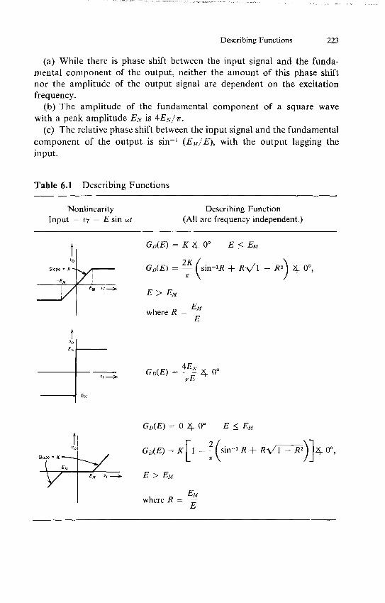
(a) While there is phase shift between the input signal and the fundamental component of the output, neither the amount of this phase shift nor the amplitude of the output signal are dependent on the excitation frequency.
(b) The amplitude of the fundamental component of a square wave with a peak amplitude EN is 4 EN7r.
(c) The relative phase shift between the input signal and the fundamental component of the output is sin- 1 (EM/E), with the output lagging the input.
Table 6.1 Describing Functions
Nonlinearity Describing Function Input = v, = E sin cor (All are frequency independent.)
GD(E) = K 4 00 E < EMI Slope= K GDE) (sin-R + RV1 - R 2) 400,
E > EM
where R Em E
V1 GD(E) = 4EN 4 0*
;b
EN
Gn(E) = 0 4 0' E EM
GD(E) = K [1 - 2sin-' R + RVR--R) 4 00,
E > EM
= Emwhere R E

224 Nonlinear Systems
Table 6.1-Continued
Nonlinearity Describing Function Input = v, = E sin wt (All are frequency independent.)
t GD(E) = 0 4 0' E < EmV0
EM GD(E) -4EN
-1 - R2 2 0* E > Em7rE EN
= Emwhere R E
E must exceed EM or a d-c term results.
4EN 1GD(E)= E2 -sin- R
7rE
= Emwhere R E
Combining these relationships shows that
GD(E) = 4EN -sin- 1 Em E > Em (6.31)irE E
GD(E) undefined otherwise
Table 6.1 lists the describing functions for several common nonlinearities. Since the transfer characteristics shown are all independent of the frequency of the input signal, the corresponding describing functions are dependent only on input-signal amplitude. While this restriction is not necessary to use describing-function techniques, the complexity associated with describing-function analysis of systems that include frequency-dependent nonlinearities often limits its usefulness.
The linearity of the Fourier series can be exploited to determine the describing function of certain nonlinearities from the known describing functions of other elements. Consider, for example, the soft-saturation characteristics shown in Fig. 6.8a. The input-output characteristics for this element can be duplicated by combining two tabulated elements as shown in

tVO Slope =
-EM
EM vi
= K 2
(a)
VI V 0
-EM E
Slope =K2
(b)
Figure 6.8 Soft saturation as a combination of two nonlinearities. (a) Transfer characteristics. (b) Decomposition into two nonlinearities.
225

226 Nonlinear Systems
Fig. 6.8b. Since the fundamental component of the output of the system of Fig. 6.8b is the sum of the fundamental components from the two nonlinearities
GD(E) =K 1 4 00 E < EM (6.32a)
GD(E) = 2K sin-IR + R V11--R2
+ K 2 - 2K2 sin-1R + R /-R2) 0
= LK2 + (K1 2) (sin-R + R - 0 (6.32b)
for E > EM, where R = sin-1 (E 1 /E).
6.3.2 Stability Analysis with the Aid of Describing Functions
Describing functions are most frequently used to determine if limit cycles (stable-amplitude periodic oscillations) are possible for a given system, and to determine the amplitudes of various signals when these oscillations are present.
Describing-function analysis is simplified if the system can be arranged in a form similar to that shown in Fig. 6.9. The inverting block is included to represent the inversion conventionally indicated at the summing point in a negative-feedback system. Since the intent of the analysis is to examine the possibility of steady-state oscillations, system input and output points are irrevelant. The important feature of the topology shown in Fig. 6.9 is
Nonlinear element
Figure 6.9 System arranged for describing-function analysis.
227 Describing Functions
that a single nonlinear element appears in a loop with a single linear element. The linear element shown can of course represent the reduction of a complex interconnection of linear elements in the original system to a single transfer function. The techniques described in Sections 2.4.2 and 2.4.3 are often useful for these reductions.
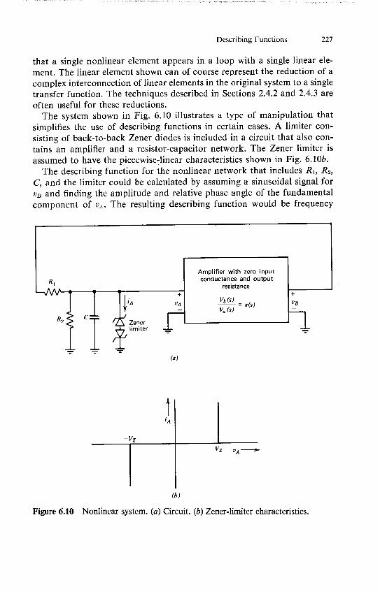
The system shown in Fig. 6.10 illustrates a type of manipulation that simplifies the use of describing functions in certain cases. A limiter consisting of back-to-back Zener diodes is included in a circuit that also contains an amplifier and a resistor-capacitor network. The Zener limiter is assumed to have the piecewise-linear characteristics shown in Fig. 6.10b.
The describing function for the nonlinear network that includes R 1, R 2, C, and the limiter could be calculated by assuming a sinusoidal signal for
and finding the amplitude and relative phase angle of the fundamental component of VA. The resulting describing function would be frequency VB
Amplifier with zero input
R, conductance and output resistance
A VA b(S) = a(s) VB
(a)
Vz A
(b)
Figure 6.10 Nonlinear system. (a) Circuit. (b) Zener-limiter characteristics.

VA
(a)
(b)
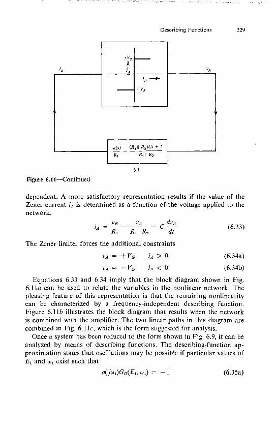
Figure 6.11 Modeling system of Fig. 6.10 as a single loop. (a) Block-diagram representation of nonlinear network. (b) Block diagram representation of complete system. (c) Reduced to form of Fig. 6.9.
228
229 Describing Functions
+Vz
a(s) (R1.11 R2)Cs + 1
R, R,\\1 R2
(c)
Figure 6.11-Continued
dependent. A more satisfactory representation results if the value of the Zener current iA is determined as a function of the voltage applied to the network.
i - VB VA -C dvA (6.33)R 1 R 1[0R 2 dt
The Zener limiter forces the additional constraints
VA = +-Vz iA > 0 (6.34a)
VA = -Vz iA < 0 (6.34b)
Equations 6.33 and 6.34 imply that the block diagram shown in Fig. 6.1la can be used to relate the variables in the nonlinear network. The pleasing feature of this representation is that the remaining nonlinearity can be characterized by a frequency-independent describing function. Figure 6.11b illustrates the block diagram that results when the network is combined with the amplifier. The two linear paths in this diagram are combined in Fig. 6.1 c, which is the form suggested for analysis.
Once a system has been reduced to the form shown in Fig. 6.9, it can be analyzed by means of describing functions. The describing-function approximation states that oscillations may be possible if particular values of Ei and coi exist such that
a(joi)GD(Ei,w i) = - 1 (6.35a)
230 Nonlinear Systems
or -l1
a(jwi) = (6.35b)GD(E1, wi)
The satisfaction of Eqn. 6.35 does not guarantee that the system in question will oscillate. It is possible that a system satisfying Eqn. 6.35 will be stable for a range of signal levels and must be triggered into oscillation by, for example, exceeding a particular signal level at the input to the nonlinear element. A second possibility is that the equality of Eqn. 6.35 does not describe a stable-amplitude oscillation. In this case, if it is assumed that the system is oscillating with parameter values given in Eqn. 6.35, a small amplitude perturbation is divergent and leads to either an increasing or a decreasing amplitude. As we shall see, the method can be used to resolve these questions. The describing-function analysis also predicts that if stable-amplitude oscillations exist, the frequency of the oscillations will be Wi and the amplitude of the fundamental component of the signal applied to the nonlinearity will be E1.
The above discussion shows how closely the describing-function stability analysis of nonlinear systems parallels the Nyquist or Bode-plot analysis of linear systems. In particular, oscillations are predicted for linear systems at frequencies where the loop transmission is -- 1, while describing-function analysis indicates possible oscillations for amplitude-frequency combinations that produce the nonlinear-system equivalent of unity loop transmission.
The basic approximation of describing-function analysis is now evident. It is assumed that under conditions of steady-state oscillation, the input to the nonlinear element consists of a single-frequency sinusoid. While this assumption is certainly not exactly satisfied because the nonlinear element generates harmonics that propagate around the loop, it is often a useful approximation for two reasons. First, many nonlinearities generate harmonics with amplitudes that are small compared to the fundamental. Second, since many linear elements in feedback systems are low-pass in nature, the harmonics in the signal returned to the nonlinear element are often attenuated to a greater degree than the fundamental by the linear elements. The second reason indicates a better approximation for higher-order low-pass systems.
The existence of the relationship indicated in Eqn. 6.35 is often determined graphically. The transfer function of the linear element is plotted in gain-phase form. The function - 1/GD(E, w) is also plotted on the same graph. If GD is frequency independent, - l/GD(E) is a single curve with E a parameter along the curve. The necessary condition for oscillation is satisfied if an intersection of the two curves exists. The frequency can be
231 Describing Functions
determined from the a(jo) curve, while amplitude of the fundamental component of the signal into the nonlinearity is determined from the - 1/GD(E) curve. If the nonlinearity is frequency dependent, a family of curves - 1/GD(E, Wi), -1/GD(E, W2), .. . , is plotted. The oscillation condition is satisfied if the -1/GD(E, cot) curve intersects the a(jw) curve at the point a(joi).
The satisfaction of Eqn. 6.35 is a necessary though not sufficient condition for a limit cycle to exist. It is also necessary to insure that the oscillation predicted by the intersection is stable in amplitude. In order to test for amplitude stability, it is assumed that the amplitude E increases slightly, and the point corresponding to the perturbed value of E is found on the - 1/GD(E, co)curve. If this point lies to the left of the a(jo) curve, the geometry implies that the system poles 3 lie in the left-half plane for an increased value of E, tending to restore the amplitude to its original value. Alternatively, if the perturbed point lies to the right of the a(jw) curve, a growing-amplitude oscillation results from the perturbation and a limit cycle with parameters predicted by the intersection is not possible. These relationships can be verified by applying the Nyquist stability test to the loop transmission, which includes the linear transfer function and the describing function of interest.
It should be noted that the stability of arbitrarily complex nonlinear systems that combine a multiplicity of nonlinear elements in a loop with linear elements can, at least in theory, be determined using describing functions. For example, numerous Nyquist plots corresponding to the nonlinear loop transmissions for a variety of signal amplitudes might be constructed to determine if the possibility for instability exists. Unfortunately, the effort required to complete this type of analysis is generally prohibitive.
6.3.3 Examples
Since describing-function analysis predicts the existence of stable-amplitude limit cycles, it is particularly useful for the investigation of oscillators, and for this reason the two examples in this section involve oscillator circuits.
The discussion of Section 4.2.2 showed that it is possible to produce sinusoidal oscillations by applying negative feedback around a phase-shift network with three identically located real-axis poles. If the magnitude of the low-frequency loop transmission is exactly 8, the system closed-loop
3The concept of a pole is strictly valid only for a linear system. Once we apply the describing-function approximation (which is a particular kind of linearization about an operating point defined by a signal amplitude), we take the same liberty with the definition of a pole as we do with systems that have been linearized by other methods.
232 Nonlinear Systems
f-+1 VB
Amplitude = E 1
oA -+1
VA -1
VB(S + 1W
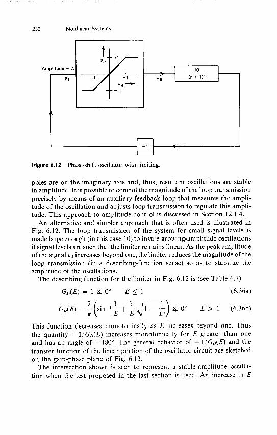
Figure 6.12 Phase-shift oscillator with limiting.
poles are on the imaginary axis and, thus, resultant oscillations are stable
in amplitude. It is possible to control the magnitude of the loop transmission
precisely by means of an auxiliary feedback loop that measures the ampli
tude of the oscillation and adjusts loop transmission to regulate this ampli
tude. This approach to amplitude control is discussed in Section 12.1.4.
An alternative and simpler approach that is often used is illustrated in Fig. 6.12. The loop transmission of the system for small signal levels is
made large enough (in this case 10) to insure growing-amplitude oscillations
if signal levels are such that the limiter remains linear. As the peak amplitude
of the signal VA increases beyond one, the limiter reduces the magnitude of the
loop transmission (in a describing-function sense) so as to stabilize the
amplitude of the oscillations. The describing function for the limiter in Fig. 6.12 is (see Table 6.1)
GD(E) = 1 4 00 E < 1 (6.36a)
GD(E) = 2(sin-1 - + - - -2) 400 E > 1 (6.36b) 7r E E E2
This function decreases monotonically as E increases beyond one. Thus
the quantity - 1/GD(E) increases monotonically for E greater than one
and has an angle of - 1800. The general behavior of - 1/GD(E) and the
transfer function of the linear portion of the oscillator circuit are sketched
on the gain-phase plane of Fig. 6.13. The intersection shown is seen to represent a stable-amplitude oscilla
tion when the test proposed in the last section is used. An increase in E
233 Describing Functions
10 W-0
1 a(jco) GD(E)
$ "|ncreasing E
increasing Io
E =1.45 w=vY
______1_1 E -270' -180' -90 '.
4 a(jw) and 4 -
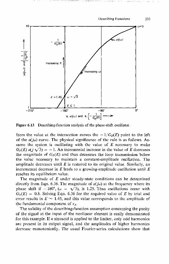
Figure 6.13 Describing-function analysis of the phase-shift oscillator.
from the value at the intersection moves the - 1/GD(E) point to the left of the a(jw) curve. The physical significance of the rule is as follows. Assume the system is oscillating with the value of E necessary to make GD(E) a(j V3) = - 1. An incremental increase in the value of E decreases the magnitude of GD(E) and thus decreases the loop transmission below the value necessary to maintain a constant-amplitude oscillation. The amplitude decreases until E is restored to its original value. Similarly, an incremental decrease in E leads to a growing-amplitude oscillation until E reaches its equilibrium value.
The magnitude of E under steady-state conditions can be determined directly from Eqn. 6.36. The magnitude of a(jo) at the frequency where its phase shift if - 1800, (w = V), is 1.25. Thus oscillations occur with GD(E) = 0.8. Solving Eqn. 6.36 for the required value of E by trial and error results in E ~_1.45, and this value corresponds to the amplitude of the fundamental component of VA.
The validity of the describing-function assumption concerning the purity of the signal at the input of the nonlinear element is easily demonstrated for this example. If a sinusoid is applied to the limiter, only odd harmonics are present in its output signal, and the amplitudes of higher harmonics decrease monotonically. The usual Fourier-series calculations show that

234 Nonlinear Systems
the ratio of the magnitude of the third harmonic to that of the fundamental at the output of the limiter is 0.14 for a 1.45-volt peak-amplitude sinusoid
as the limiter input. The linear elements attenuate the third harmonic of
a V radian-per-second sinusoid by a factor of 18 greater than the fundamental. Thus the ratio of third harmonic to fundamental is approximately 0.008 at the input to the nonlinear element. The amplitudes of higher harmonics are insignificant since their magnitudes at the limiter output are
smaller and since they are attenuated to a greater extent by the linear ele
ment. As a matter of practical interest, the attenuation provided by the
phase-shift network to harmonics is the reason that good design practice dictates the use of the signal out of the phase-shift network rather than that from the limiter as the oscillator output signal.
Figure 6.14a shows another oscillator configuration that is used as a
second example of describing-function analysis. This circuit, which com
bines a Schmitt trigger and an integrator, is a simplified representation of
that used in several commercially available function generators. It can be
shown by direct evaluation that the signal at the input to the nonlinear
element is a two-volt peak-to-peak triangle wave with a four-second period
and that the signal at the output of the nonlinear element is a two-volt
peak-to-peak square wave at the same frequency. Zero crossings of these
two signals are displaced by one second as shown in Fig. 6.14b. The ratio
of the third harmonic to the fundamental at the input to the nonlinear element is 1/9, a considerably higher value than in the previous example.
Table 6.1 shows that the describing function for this nonlinearity is
4 1 GD(E) = -sin-' E > 1 (6.37)
rE E
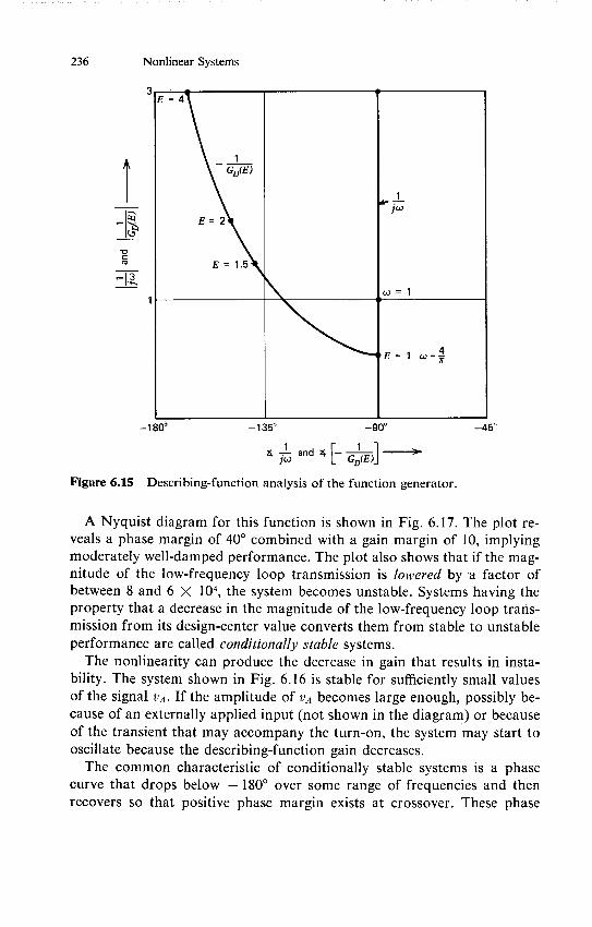
The quantity - 1 GD(E) and the transfer function for the linear element are
plotted in gain-phase form in Fig. 6.15. The intersection occurs for a value
of E that results in the maximum phase lag of 90' from the nonlinear ele
ment. The parameters predicted for the stable-amplitude limit cycle im
plied by this intersection are a peak-to-peak amplitude for vA of two volts
and a period of oscillation of approximately five seconds. The correspond
ence between these parameters and those of the exact solution is excellent
considering the actual nature of the signals involved.
6.3.4 Conditional Stability
The system shown in block-diagram form in Fig. 6.16 combines a satu
rating nonlinearity with linear elements. The negative of the loop trans

235 Describing Functions
vAA
Schmitt trigger provides hysteresis.
(a)
+1 V
A VA
tso (seconds)
-1 V
+1 V
VtVB II I I I I I 0 3 4 5 6 71 2 ts
(seconds)
-1 V I (b)
Figure 6.14 Function generator. (a) Configuration. (b) Waveforms.
mission for this system, assuming that the amplitude of the signal at VA is less than 10- volts so that the nonlinearity provides a gain of 10, is determined by breaking the loop at the inverting block, yielding
-L(s) = 105a(s) = 5 X 10⁵(0.02s + 1)2 (6.38)(s + 1)3(10- 3s + 1)2
236 Nonlinear Systems
I GD(E)1
E = 2
C E =1.5
11
E =1 4
-180* -135* -90* -45*
4 and 4
Figure 6.15 Describing-function analysis of the function generator.
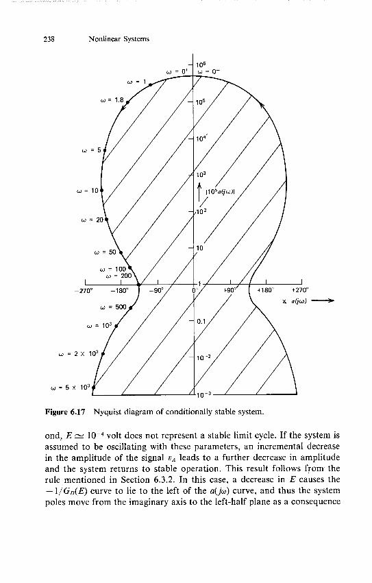
A Nyquist diagram for this function is shown in Fig. 6.17. The plot reveals a phase margin of 40* combined with a gain margin of 10, implying moderately well-damped performance. The plot also shows that if the magnitude of the low-frequency loop transmission is lowered by a factor of between 8 and 6 X 10⁴, the system becomes unstable. Systems having the property that a decrease in the magnitude of the low-frequency loop transmission from its design-center value converts them from stable to unstable performance are called conditionallystable systems.
The nonlinearity can produce the decrease in gain that results in instability. The system shown in Fig. 6.16 is stable for sufficiently small values of the signal VA. If the amplitude of VA becomes large enough, possibly because of an externally applied input (not shown in the diagram) or because of the transient that may accompany the turn-on, the system may start to oscillate because the describing-function gain decreases.
The common characteristic of conditionally stable systems is a phase curve that drops below - 1800 over some range of frequencies and then recovers so that positive phase margin exists at crossover. These phase
237 Describing Functions
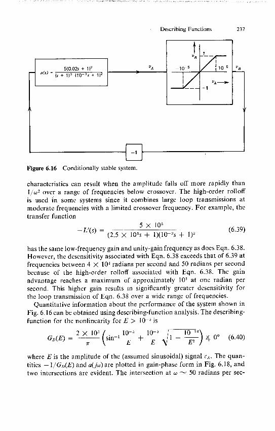
Figure 6.16 Conditionally stable system.
characteristics can result when the amplitude falls off more rapidly than 1/o 2 over a range of frequencies below crossover. The high-order rolloff is used in some systems since it combines large loop transmissions at moderate frequencies with a limited crossover frequency. For example, the transfer function
5 X 10⁵ -L'(s) 5X1 -(6.39)
(2.5 X 10³s + 1)(10- 3s + 1)2
has the same low-frequency gain and unity-gain frequency as does Eqn. 6.38. However, the desensitivity associated with Eqn. 6.38 exceeds that of 6.39 at frequencies between 4 X 10⁴ radians per second and 50 radians per second because of the high-order rolloff associated with Eqn. 6.38. The gain advantage reaches a maximum of approximately 10 at one radian per second. This higher gain results in significantly greater desensitivity for the loop transmission of Eqn. 6.38 over a wide range of frequencies.
Quantitative information about the performance of the system shown in Fig. 6.16 can be obtained using describing-function analysis. The describing-function for the nonlinearity for E > 10-5 is
2 X 10⁵ 10-5 10-5 10-1 GD(E)- (sin-i - + 1 -- E2) 400 (6.40)
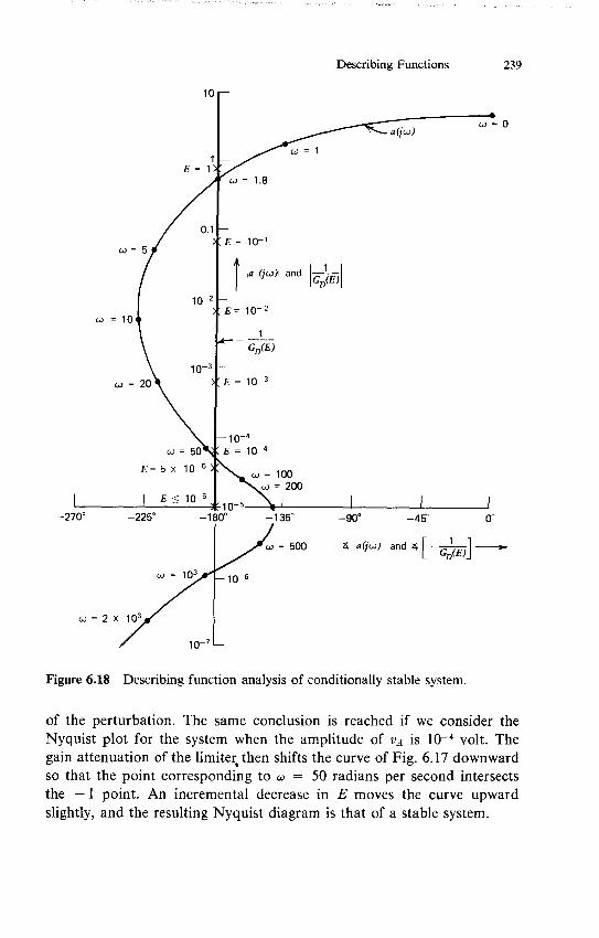
where E is the amplitude of the (assumed sinusoidal) signal VA. The quantities - 1/GD(E) and a(jo) are plotted in gain-phase form in Fig. 6.18, and two intersections are evident. The intersection at co 50 radians per sec
238 Nonlinear Systems
w = Z X IU- - 10-2
= 5 x 11 30
Figure 6.17 Nyquist diagram of conditionally stable system.
ond, E ~_ 10-4 volt does not represent a stable limit cycle. If the system is
assumed to be oscillating with these parameters, an incremental decrease in the amplitude of the signal VA leads to a further decrease in amplitude
and the system returns to stable operation. This result follows from the
rule mentioned in Section 6.3.2. In this case, a decrease in E causes the
- 1/GD(E) curve to lie to the left of the a(jw) curve, and thus the system
poles move from the imaginary axis to the left-half plane as a consequence
239 Describing Functions
10
a(jw)
E = 1 = 1.8
. = 5 10-1
Ila (jw) and GD(E)
10- 2 ( = 10
GD(E)
w = 20
10-4
o = 100 = 200
-270' -225' 135* -90* -45' 0
= 500 4 a(jw) and 4 [- 1
-6
=2 x 10³ /
Figure 6.18 Describing function analysis of conditionally stable system.
of the perturbation. The same conclusion is reached if we consider the Nyquist plot for the system when the amplitude of VA is 10-4 volt. The gain attenuation of the limiter then shifts the curve of Fig. 6.17 downward so that the point corresponding to co = 50 radians per second intersects the - 1 point. An incremental decrease in E moves the curve upward slightly, and the resulting Nyquist diagram is that of a stable system.
240 Nonlinear Systems
Similar reasoning shows that a small increase in amplitude at the lower intersection leads to further increases in amplitude. Following this type of perturbation, the system eventually achieves the stable-amplitude limit cycle implied by the upper intersection with w - 1.8 radians per second and E - 0.73 volt. (The reader should convince himself that the upper intersection satisfies the conditions for a stable-amplitude limit cycle.)
It should be noted that the concept of conditionally stable behavior aids in understanding the large-signal performance of systems for which the phase shift approaches but does not exceed 1800 well below crossover, and then recovers to a more reasonable value at crossover. While these systems can exhibit excellent performance for signal levels that constrain operation to the linear region, performance generally deteriorates dramatically when some element in the loop saturates. For example, the recovery of this type of system following a large-amplitude step may include a number of large-signal overshoots, even if the small-signal step response of the system is approximately first order.
Although a detailed analysis of such behavior is beyond the scope of this book, examples of the large-signal performance of systems that approach conditional stability are included in Chapter 13.
6.3.5 Nonlinear Compensation
As we might suspect, the techniques for compensating nonlinear systems using either linear or nonlinear compensating networks are not particularly well understood. The method of choice is frequently critically dependent on exact details of the linear and nonlinear elements included in the loop. In some cases, describing-function analysis is useful for indicating compensation approaches, since systems with greater separation between the a(jo) and - 1/GD(E) curves are generally relatively more stable. This section outlines one specific method for the compensation of nonlinear systems.
As mentioned earlier, fast-rolloff loop transmissions are used because of the large magnitudes they can yield at intermediate frequencies. Unfortunately, if the phase shift of this type of loop transmission falls below - 1800 at a frequency where its magnitude exceeds one, conditional stability can result. Nonlinear compensation can be used to eliminate the possibility of oscillations in certain systems with this type of loop transmission.
As one example, consider a system with a linear-region loop transmission
200 -L(s) = 20(6.41)
(s + 1)(10- 3s + 1)2
This loop transmission has a monotonically decreasing phase shift as a function of increasing frequency, and exhibits a phase margin of approxi
241 Describing Functions
mately 650. Consequently, unconditional stability is assured even when some element in the loop saturates.
In an attempt to improve the desensitivity of the system, series compensation consisting of gain and two lag transfer functions might be added to the loop transmission of Eqn. 6.41, leading to the modified loop transmission
200 2.5 X 10³(0.02s + 1)2 (6.42) (s -+ 1)(10- 3 s + )2_] (s + 1)2 j
This loop transmission is of course the one used to illustrate the possibility of conditional stability (Eqn. 6.38).
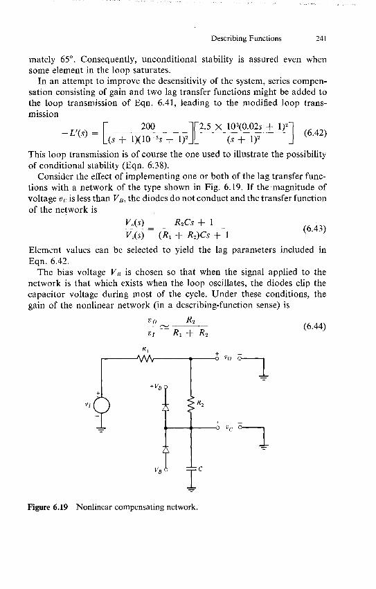
Consider the effect of implementing one or both of the lag transfer functions with a network of the type shown in Fig. 6.19. If the magnitude of voltage yc is less than VB, the diodes do not conduct and the transfer function of the network is
V6(s) R 2Cs + 1 Vi(s) (R 1 + R 2)Cs + 1
Element values can be selected to yield the lag parameters included in Eqn. 6.42.
The bias voltage VB is chosen so that when the signal applied to the network is that which exists when the loop oscillates, the diodes clip the capacitor voltage during most of the cycle. Under these conditions, the gain of the nonlinear network (in a describing-function sense) is
vo * R2 (6.44) or R1 + R2
R +
V0 C
+ VB
VI R2
++
Figure 6.19 Nonlinear compensating network.
242 Nonlinear Systems
Note that if both lag transfer functions are realized this way, the loop transmission can be made to automatically convert from that given by Eqn. 6.42 to that of Eqn. 6.41 under conditions of impending instability. This type of compensation can eliminate the possibility of conditionally stable performance in certain systems. The signal levels that cause saturation also remove the lag functions, and thus the possibility of instability can be eliminated.
PROBLEMS
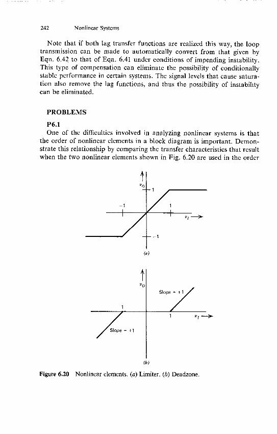
P6.1 One of the difficulties involved in analyzing nonlinear systems is that
the order of nonlinear elements in a block diagram is important. Demonstrate this relationship by comparing the transfer characteristics that result when the two nonlinear elements shown in Fig. 6.20 are used in the order
'o
-1 1
- -1
(a)
t V
0
Slope = +1
Slope = +1
(b)
Figure 6.20 Nonlinear elements. (a) Limiter. (b)Deadzone.

Problems 243
00E OE
Resolver pair
Figure 6.21 Positional servomechanism.
ab with the transfer characteristics that result when the order is changed to ba.
P6.2 Resolvers are essentially variable transformers that can be used as
mechanical-angle transducers. When two of these devices are used in a servomechanism, the voltage obtained from the pair is a sinusoidal function of the difference between the input and output angles of the system. A model for a servomechanism using resolvers is shown in Fig. 6.21. (a) The voltage applied to the amplifier-motor combination is zero for
Oo - 0r = nir, where n is any integer. Use linearized analysis to determine which of these equilibrium points are stable.
(b) The system is driven at a constant input velocity of 7 radians per second. What is the steady-state error between the output and input for this excitation?
R
VO C,_I
VI
VB VA
Figure 6.22 Square-rooting circuit.
244 Nonlinear Systems
(c) The input rate is charged from 7 to 7.1 radians per second in zero time. Find the corresponding output-angle transient.
P6.3 An analog divider was described in Section 6.2.2. Assume that the trans
fer function of the operational amplifier shown in Fig. 6.2 is
3 X 101 + 1)2(s + 1)(10-Is
Is the divider stable over the range of inputs - 10 < VA < + 10, 0 < VB <
+10? A square-rooting circuit using a technique similar to that of the divider
is shown in Fig. 6.22. What is the ideal input-output relationship for this circuit? Determine the range of input voltages for which the square-rooter is stable, assuming a(s) is as given above.
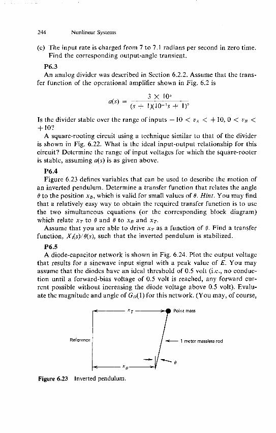
P6.4 Figure 6.23 defines variables that can be used to describe the motion of
an inverted pendulum. Determine a transfer function that relates the angle 0 to the position XB, which is valid for small values of 6. Hint. You may find that a relatively easy way to obtain the required transfer function is to use the two simultaneous equations (or the corresponding block diagram) which relate XT to 6 and 6 to XB and XT.
Assume that you are able to drive XT as a function of 6. Find a transfer function, X,(s)/6(s), such that the inverted pendulum is stabilized.
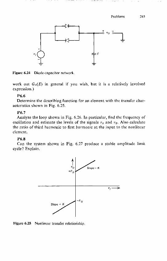
P6.5 A diode-capacitor network is shown in Fig. 6.24. Plot the output voltage
that results for a sinewave input signal with a peak value of E. You may assume that the diodes have an ideal threshold of 0.5 volt (i.e., no conduction until a forward-bias voltage of 0.5 volt is reached, any forward current possible without increasing the diode voltage above 0.5 volt). Evaluate the magnitude and angle of GD(1) for this network. (You may, ofcourse,
XT Point mass
Reference - 1 meter massless rod
0 MeXB-K
Figure 6.23 Inverted pendulum.
Problems 245
CVO O'3-1
YI
Figure 6.24 Diode-capacitor network.
work out GD(E) in general if you wish, but it is a relatively involved expression.)
P6.6 Determine the describing function for an element with the transfer char
acteristics shown in Fig. 6.25.
P6.7 Analyze the loop shown in Fig. 6.26. In particular, find the frequency of
oscillation and estimate the levels of the signals VA and vB. Also calculate the ratio of third harmonic to first harmonic at the input to the nonlinear element.
P6.8 Can the system shown in Fig. 6.27 produce a stable amplitude limit
cycle? Explain.
vlp = K
+EN
SEN Slope = K
Figure 6.25 Nonlinear transfer relationship.
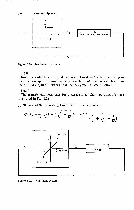
246 Nonlinear Systems
V
VA VB (s -10 VA d (S+ 1)(0.1 S+ 1)(0.01 S+1
Figure 6.26 Nonlinear oscillator.
P6.9 Find a transfer function that, when combined with a limiter, can pro
duce stable-amplitude limit cycles at two different frequencies. Design an operational-amplifier network that realizes your transfer function.
P6.10 The transfer characteristics for a three-state, relay-type controller are
illustrated in Fig. 6.28.
(a) Show that the describing function for this element is
GD(E) = 2 2 + 2 11 42 -tan-' rE 2 n (I+E 1-I
Slope = +2
vB
1 -
va VB_ -5
(rs + 1)3I 1 -' -
Slope = +2
Figure 6.27 Nonlinear system.
Problems 247
Vf 0
-1 V I >
1
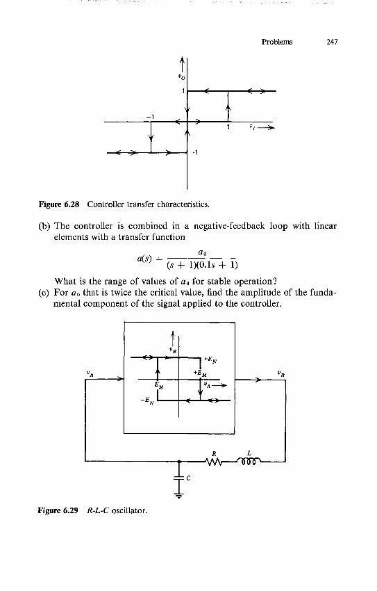
Figure 6.28 Controller transfer characteristics.
(b) The controller is combined in a negative-feedback loop with linear elements with a transfer function
a(s) = ao (s + 1)(0.Is + 1)
What is the range of values of ao for stable operation? (c) For ao that is twice the critical value, find the amplitude of the funda
mental component of the signal applied to the controller.
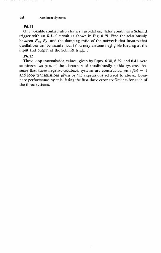
f VB
+EN
VBVA +EM
-EM VA
-EN
R L
C
Figure 6.29 R-L-C oscillator.
248 Nonlinear Systems
P6.11 One possible configuration for a sinusoidal oscillator combines a Schmitt
trigger with an R-L-C circuit as shown in Fig. 6.29. Find the relationship between Em, EN, and the damping ratio of the network that insures that oscillations can be maintained. (You may assume negligible loading at the input and output of the Schmitt trigger.)
P6.12 Three loop-transmission values, given by Eqns. 6.38, 6.39, and 6.41 were
considered as part of the discussion of conditionally stable systems. Assume that three negative-feedback systems are constructed with f(s) = 1 and loop transmissions given by the expressions referred to above. Compare performance by calculating the first three error coefficients for each of the three systems.

MIT OpenCourseWarehttp://ocw.mit.edu
RES.6-010 Electronic Feedback SystemsSpring 2013
For information about citing these materials or our Terms of Use, visit: http://ocw.mit.edu/terms.