October 1998

NASA/CR-1998-208721

Operational Data Reduction Procedure forDetermining Density and Vertical Structure ofthe Martian Upper Atmosphere From MarsGlobal Surveyor Accelerometer Measurements

George J. Cancro, Robert H. Tolson, and Gerald M. KeatingThe George Washington UniversityJoint Institute for Advancement of Flight SciencesLangley Research Center, Hampton, Virginia

The NASA STI Program Office ... in Profile

Since its founding, NASA has been dedicatedto the advancement of aeronautics and spacescience. The NASA Scientific and TechnicalInformation (STI) Program Office plays a keypart in helping NASA maintain thisimportant role.

The NASA STI Program Office is operated byLangley Research Center, the lead center forNASAÕs scientific and technical information.The NASA STI Program Office providesaccess to the NASA STI Database, thelargest collection of aeronautical and spacescience STI in the world. The Program Officeis also NASAÕs institutional mechanism fordisseminating the results of its research anddevelopment activities. These results arepublished by NASA in the NASA STI ReportSeries, which includes the following reporttypes: · TECHNICAL PUBLICATION. Reports of

completed research or a major significantphase of research that present the resultsof NASA programs and include extensivedata or theoretical analysis. Includescompilations of significant scientific andtechnical data and information deemedto be of continuing reference value. NASAcounter-part of peer reviewed formalprofessional papers, but having lessstringent limitations on manuscriptlength and extent of graphicpresentations.

· TECHNICAL MEMORANDUM.

Scientific and technical findings that arepreliminary or of specialized interest,e.g., quick release reports, workingpapers, and bibliographies that containminimal annotation. Does not containextensive analysis.

· CONTRACTOR REPORT. Scientific and

technical findings by NASA-sponsoredcontractors and grantees.

· CONFERENCE PUBLICATION.

Collected papers from scientific andtechnical conferences, symposia,seminars, or other meetings sponsored orco-sponsored by NASA.

· SPECIAL PUBLICATION. Scientific,

technical, or historical information fromNASA programs, projects, and missions,often concerned with subjects havingsubstantial public interest.

· TECHNICAL TRANSLATION. English-

language translations of foreign scientificand technical material pertinent toNASAÕs mission.

Specialized services that help round out theSTI Program OfficeÕs diverse offerings includecreating custom thesauri, building customizeddatabases, organizing and publishingresearch results ... even providing videos.

For more information about the NASA STIProgram Office, see the following:

· Access the NASA STI Program HomePage at http://www.sti.nasa.gov

· E-mail your question via the Internet to

help@sti.nasa.gov · Fax your question to the NASA Access

Help Desk at (301) 621-0134 · Phone the NASA Access Help Desk at

(301) 621-0390 · Write to:

NASA Access Help Desk NASA Center for AeroSpace Information 7121 Standard Drive Hanover, MD 21076-1320

National Aeronautics andSpace Administration

Langley Research Center Prepared for Langley Research CenterHampton, Virginia 23681-2199 under Cooperative Agreement NCC1-104

October 1998

NASA/CR-1998-208721

Operational Data Reduction Procedure forDetermining Density and Vertical Structure ofthe Martian Upper Atmosphere From MarsGlobal Surveyor Accelerometer Measurements

George J. Cancro, Robert H. Tolson, and Gerald M. KeatingThe George Washington UniversityJoint Institute for Advancement of Flight SciencesLangley Research Center, Hampton, Virginia

Available from the following:

NASA Center for AeroSpace Information (CASI) National Technical Information Service (NTIS)7121 Standard Drive 5285 Port Royal RoadHanover, MD 21076-1320 Springfield, VA 22161-2171(301) 621-0390 (703) 487-4650

i

Abstract

The success of aerobraking at Mars by the Mars Global Surveyor (MGS)

spacecraft was partly due to the analysis of MGS accelerometer data. Accelerometer data

was used to determine the effect of the atmosphere on each orbit, to characterize the

nature of the atmosphere, and to predict the atmosphere for future orbits. To properly

interpret the accelerometer data, a data reduction procedure was developed which utilizes

inputs from the spacecraft, the MGS Navigation Team, and pre-mission

aerothermodynamic studies to produce density estimations at various points and altitudes

on the planet. This data reduction procedure was based on the calculation of acceleration

due to aerodynamic forces from the accelerometer data by considering acceleration

components due to gravity gradient, solar pressure, angular motion of the instrument,

instrument bias, thruster activity, and a vibration component due to the motion of the

damaged solar array. Methods were developed to calculate all of the acceleration

components including a 4 degree of freedom dynamics model used to gain a greater

understanding of the damaged solar array. An iteration process was developed to

calculate density by calculating deflection of the damaged array and a variable force

coefficient. The total error inherent to the data reduction procedure was calculated as a

function of altitude and density considering contributions from ephemeris errors, errors in

force coefficient, and instrument errors due to bias and digitization. Comparing the results

from this procedure to the data of other MGS Teams has demonstrated that this procedure

can quickly and accurately describe the density and vertical structure of the Martian upper

atmosphere.

ii

iii

Table of Contents

Abstract...........................................................................................................................i

Table of Contents..........................................................................................................iii

List of Figures................................................................................................................v

List of Tables ...............................................................................................................vii

Nomenclature..............................................................................................................viii

1. Introduction...............................................................................................................1

2. MGS Aerobraking Scenario......................................................................................3

2.1 Accelerometer Instrument.......................................................................................3

2.2 MGS Aerobraking Configuration............................................................................3

2.3 Complexities of the MGS Aerobraking Mission......................................................4

2.4 Accelerometer Team Responsibilities......................................................................6

2.5 Description of Panel Malfunction............................................................................8

3. Analysis of Acceleration Data.................................................................................10

3.1 Development of the Acceleration Term.................................................................10

3.2 Development of the Spacecraft Velocity Term......................................................21

3.3 Development of the Ballistic Coefficient Term......................................................22

4. Operational Data Reduction Procedure.................................................................28

4.1 Operational Constraints........................................................................................28

4.2 Operational Accelerometer Instrument..................................................................29

4.3 Quantity of Accelerometer Data Necessary to Perform Operations........................31

4.4 Operational Data Reduction Process.....................................................................34

4.5 Special Products...................................................................................................40

4.6 Prediction Methods...............................................................................................43

5. Analysis of Process Errors.......................................................................................45

5.1 Ephemeris Errors..................................................................................................45

5.2 Errors in Determining Ballistic Coefficient............................................................46

5.3 Errors in Determining Bias....................................................................................47

iv

5.4 Errors due to Instrument Output...........................................................................48

5.5 Total Data Reduction Process Error .....................................................................49

6. Verification of Accelerometer Results.....................................................................51

6.1 Data Reduction Process Verification.....................................................................51

6.2 Prediction Scheme Verification.............................................................................54

7. The Effect of Panel Vibration on MGS and the Accelerometer Data Reduction

Process..........................................................................................................................57

7.1 Effectiveness of the 4 DOF Dynamics Model........................................................58

7.2 Verification of the Dynamics Model And Assumptions..........................................59

7.3 Sensitivity Studies on Panel Physical Parameters...................................................61

7.4 Averaging Techniques Used to Compensate for Vibrating Panel Effects................64

8. Conclusions..............................................................................................................65

References....................................................................................................................67

APPENDIX A: Description of Quick-Look Data Product .........................................69

APPENDIX B: 4 DOF Derivation for Eliminating SAM panel Motions from Z-

Accelerometer Data...........................................................................74

APPENDIX C: LaRC Aerothermodynamic Database for MGS Operations............80

APPENDIX D: Planetary Ephemeris and Physical Data...........................................89

APPENDIX E: MGS Physical Properties...................................................................90

APPENDIX F: Verification of 4 DOF Model Derivation ...........................................91

v

List of Figures

Figure 2-1: MGS aerobraking configuration...................................................................4

Figure 2-2: Diagram of basic MGS project team relationships........................................7

Figure 2-3: Spare yoke with suspected failure mode.......................................................9

Figure 3-1: Typical spacecraft angular rates (Orbit 162)...............................................16

Figure 3-2: Typical x, y and z angular accelerations (Orbit 162)...................................16

Figure 3-3: Typical thruster fire times (Orbit 16)..........................................................18

Figure 3-4: Acceleration data with large amplitude vibrations (Orbit 95)......................19

Figure 3-5: Diagram of 2-body 4 DOF model used to estimate moving panel

acceleration ..............................................................................................19

Figure 3-6: Ux and Uy coordinate definition................................................................23

Figure 3-7: Force coefficient in spacecraft z-direction, Cz, vs. density level for all

panel deflections .......................................................................................24

Figure 3-8: Cz tables for free molecular densities (0 degree SAM Deflection and 10

degree SAM Deflection) ...........................................................................25

Figure 3-9: Typical quaternions (Orbit 162).................................................................26

Figure 3-10: Typical Ux and Uy diagram (Orbit 162).....................................................27

Figure 4-1: Typical IMU temperatures and voltage to IMU heater (Orbit 162).............30

Figure 4-2: Results of Accelerometer Data Rate Simulation.........................................32

Figure 4-3: Results of accelerometer data rate simulation considering all possible

outcomes ..................................................................................................33

Figure 4-4: Data reduction process flow chart..............................................................34

Figure 4-5: Typical accelerometer instrument bias calculation......................................36

Figure 4-6: Development of density flow chart.............................................................37

Figure 4-7: Typical z-force coefficient and panel deflection from Orbit 162..................38

Figure 4-8: Comparison of the operational averaging techniques..................................39

Figure 4-9: Look-ahead model diagram........................................................................44

Figure 5-1: Accelerometer process error vs. model altitude and density.......................50

vi

Figure 6-1: Comparison of panel position calculated using accelerometer data and sun

sensor data.................................................................................................52

Figure 6-2: Orbital decay comparison of NAV and ACC using ρ HS product ..............53

Figure 6-3: Comparison of effectiveness of persistence, 5-orbit mean, longitudinal

wave, and look ahead prediction schemes over Orbits 100-200 ..................55

Figure 7-1: Acceleration profiles for Orbit 162 - raw data, reduced data using

4 DOF model, and reduced data using band-pass filtering method..............58

Figure 7-2: Acceleration profiles for Orbit 95 - raw data, reduced data using

4 DOF model, and reduced data using band-pass filtering method..............59

Figure 7-3: Sensitivity study on SAM moment of inertia about the spacecraft

x-axis at the SAM center of mass...............................................................62

Figure 7-4: Sensitivity study on SAM mass...................................................................62

Figure 7-5: Sensitivity study on SAM center of gravity position....................................63

Figure 7-6: Sensitivity study on crack-line position........................................................63

Figure 7-7: Comparision between 4 DOF dynamics model and 40 pt (left) and

6 pt running means (right) for Orbit 162.....................................................64

vii

List of Tables

Table 3-1: Aerodynamic Force Acceleration Simulation Results....................................11

Table 3-2: Gravity Gradient Acceleration Simulation Results........................................13

Table 3-3: Results of Range Error Study Between Exact Ephemeris and Ephemeris

Generated From Osculating Elements at Periapsis........................................22

Table 4-1: Telemetry Data Types And Rates For Operations.........................................29

Table 4-2: Results From Reliability of Accelerometer Data Simulation..........................33

Table 5-1: Total Altitude Error Results.........................................................................46

Table 5-2: Ephemeris Timing Error Results for 0.1 Seconds of Timing Error................46

Table 5-3: Bias Percent Error as a Function of Count Level..........................................48

Table 5-4: Quantization and Data Rate Error Results....................................................48

Table 5-5: Total Data Reduction Process Error.............................................................49

Table 6-1: Results of NAV Simulation Runs with Accelerometer Calculated

Effective Scale Height.................................................................................54

Table 7-1: Crack-Line Position and Resulting Physical Parameters

for Sensitivity Study....................................................................................61

viii

Nomenclature

αsun = right ascension of the sun in Mars equatorial coordinates, rad

αs/c = right ascension of the spacecraft in Mars equatorial coordinates, rad

α = angular acceleration of the spacecraft, rad/s2

A = spacecraft reference area, 17.03 m2

ACC = Accelerometer

ADL = Atmospheric Disturbance Level

a,e,i,w,Ω,τ = Keplerian orbital elements: semi-major axis, eccentricity, inclination,

argument of periapsis, longitude of ascending node, time of periapsis

az = acceleration due to aerodynamic forces in spacecraft z-axis, m/s2

azBP= band-pass filtered z-axis acceleration, m/s2

BUS = spacecraft main body

C1 , C2 = parameters of band-pass filter

Cx Cy Cz = force coefficients in the spacecraft x, y, z axes, respectively

CMx CMy CMz = moment coefficients about the spacecraft x, y, z axes, respectively

c = speed of light, 3*108 m/s

δsun = declination of the sun in Mars equatorial coordinates, rad

δs/c = declination of the spacecraft in Mars equatorial coordinates, rad

DCM = Direction Cosine Matrix

DOF = Degrees Of Freedom

∆R = areocentric distance to accelerometer instrument, km

∆r, ∆θ, ∆z = cylindrical components of ∆R

ETC = Ephemeris Timing Correction

Fs = solar constant, 590 W/m2 at Mars

f = true anomaly

fm = flattening of Mars

g = acceleration of gravity on Mars surface, 3.4755 m/s2

HGA = High Gain Antenna

ix

HS = scale height, km

h = angular momentum of an orbit, km2/s

IMU = Inertial Measurement Unit

L = longitude, deg

L = rotation rate of Mars, deg/day

LMA = Lockheed Martin Astronautics

LST = Local Solar Time, Martian hrs

µ = gravitational constant for Mars, 42828 km3/s2

m = spacecraft mass, kg

MGS = Mars Global Surveyor

NAV = Navigation

ω = angular velocity of the spacecraft, rad/s

ρ = density, kg/km3

ρ0 = base density, kg/km3

Q = free stream heat flux, W/cm2

q = dynamic pressure, N/m2

qr = reflectance factor for solar pressure

q1, q2, q3, q4 = spacecraft quaternions

R = areocentric distance to accelerometer instrument, km

Rcm = areocentric distance to spacecraft center of mass, km

R,θ,Ζ = cylindrical orbit coordinates: distance from planet, angular distance

along orbit path, distance perpindicular to orbit path

rcm = radial distance from Mars center to spacecraft center of mass, km

SAM = Solar Array Minus (on -Y spacecraft axis)

SAP = Solar Array Plus (on +Y spacecraft axis)

SZA = Solar Zenith Angle, deg

S/C = Spacecraft

θ = angular velocity in orbit plane, deg/s

θδ = deflection angle of the damaged solar array, deg

x

θi = Incidence angle of solar radiation, deg

θL = areocentric latitude, deg

θL’ = areodetic latitude, deg

T = spring torque, in-lbs

T0 = base temperature, K

T1 = temperature change with altitude, K/km

TCM = Trajectory Correction Maneuver

Ux,Uy = direction sines describing the orientation of the relative wind with

respect to the spacecraft x and y axes

v = orbital velocity of spacecraft, km/s

z = areodetic altitude, km

z0 = base altitude, km

1

1. Introduction

The Mars Global Surveyor (MGS) spacecraft is NASA’s first orbiter to return to

the red planet in 20 years. MGS represents the first project in the NASA Mars Surveyor

Program, a series of missions to Mars every 25 months over a period of 10 years. The

goals of the Mars Surveyor Program are to analyze the physical and atmospheric

properties of the planet and gain a greater understanding of how Mars formed [1]. The

MGS mission begins this analysis by achieving the following science goals:

(1) Successfully characterize the gravity field and surface properties of the planet,

(2) Establish the nature of the magnetic field, and

(3) Monitor the global structure of the atmosphere [2].

To accomplish these goals while maintaining a low budget, a technique called

“aerobraking” was planned to position the MGS spacecraft close enough to the planet for

onboard science instruments to properly collect data. Aerobraking is the process of using

atmospheric drag to remove kinetic energy from an orbit. The MGS spacecraft used

repeated encounters with the atmosphere (aerobraking passes) to gradually change a long

period-high eccentricity orbit to a short period-low eccentricity orbit. By relying on

multiple aerobraking passes instead of propulsive maneuvers to modify the orbit, less fuel

was needed during the MGS mission and, therefore, the design weight of the spacecraft

was reduced.

Aerobraking had to be monitored during each pass through the atmosphere to

ensure the safety of the spacecraft and the effectiveness of the technique. To monitor

aerobraking, Keating et al. [Keating, G.M., Tolson, R.H., Bougher S.W., Blanchard R.C.,

“MGS Accelerometer Proposal for JPL Operations, Dec 1995. Available from author]

proposed the use of on-board accelerometer data to produce density estimations as a

function of altitude for each pass and density predictions for future passes. In accord with

this proposal, a data reduction procedure was created. This paper presents the data

reduction procedure and demonstrates the effectiveness of this procedure in calculating

2

and predicting densities for 149 aerobraking orbits completed by MGS. These 149 orbits

occurred during the first 201 orbits at Mars, called the 1st phase of aerobraking.

First, this paper discusses the MGS aerobraking scenario including descriptions of

the accelerometers, the MGS spacecraft and the malfunction of one of the solar arrays on

the spacecraft. Next, the relationship between atmospheric density and acceleration due to

aerodynamic forces is examined. Methods were developed to determine each of the

components of this relationship. One such method is a dynamics model designed to

compensate for the effects of the damaged solar array on the measured acceleration.

These methods are combined with an iterative process to form the data reduction

procedure which determines density from accelerometer data. The errors inherent to the

data reduction procedure are calculated by considering ephemeris errors, force coefficient

errors, and instrument errors. The data reduction procedure is verified using panel

deflection data determined by the MGS Spacecraft Team and orbital period reduction data

generated by the MGS Navigation Team.

Finally, the methods developed in this report are used to give a greater insight into

the solar array malfunction. The dynamics model mentioned briefly above, successfully

compensates for 90% of vibration signal associated with the solar array malfunction.

Sensitivity studies were performed using the dynamics model to determine the source of

the remaining 10%.

3

2. MGS Aerobraking Scenario

This section will describe the key elements of the MGS aerobraking scenario

including the accelerometer instrument, the aerobraking configuration, the complexities of

aerobraking at Mars, and the role of the team monitoring the aerobraking process using

on-board accelerometer data.

During deployment, one of the two solar arrays on the MGS spacecraft

malfunctioned. This section also gives a brief description of this malfunction and how the

malfunction effects the analysis of accelerometer data.

2.1 Accelerometer Instrument

The MGS accelerometers are instruments that measure the change in velocity of

the spacecraft over a time interval by measuring the fluctuations of voltage to an

electromagnetic assembly. The assembly is essentially a magnetic proof mass suspended

on a thin flexure in an electromagnetically charged ring. When the spacecraft accelerates,

the position of the proof mass inside the ring is maintained by varying the voltage. After

the instrument is calibrated in a known g-field, the acceleration of the spacecraft can be

calculated by recording the change in voltage to the ring.

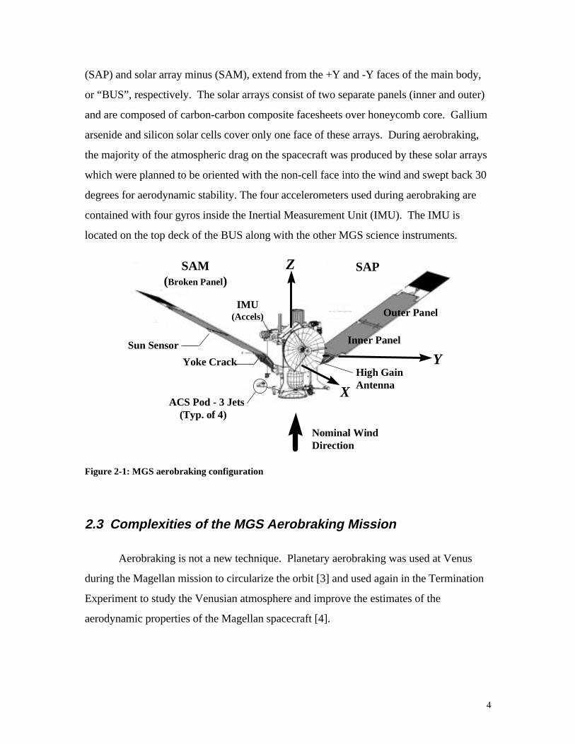
2.2 MGS Aerobraking Configuration

Several minutes before beginning the aerobraking pass through the Martian

atmosphere, the MGS spacecraft was placed in the aerobraking configuration. The

aerobraking configuration, shown in Figure 2-1, consists of the spacecraft oriented with

the main engine nozzle (spacecraft -z axis) pointed in the direction of spacecraft motion or

the “velocity vector” and the High Gain Antenna (spacecraft x axis) pointed toward the

planet,“nadir”, or away from the planet,”zenith”. The two solar arrays, solar array plus

4

(SAP) and solar array minus (SAM), extend from the +Y and -Y faces of the main body,

or “BUS”, respectively. The solar arrays consist of two separate panels (inner and outer)

and are composed of carbon-carbon composite facesheets over honeycomb core. Gallium

arsenide and silicon solar cells cover only one face of these arrays. During aerobraking,

the majority of the atmospheric drag on the spacecraft was produced by these solar arrays

which were planned to be oriented with the non-cell face into the wind and swept back 30

degrees for aerodynamic stability. The four accelerometers used during aerobraking are

contained with four gyros inside the Inertial Measurement Unit (IMU). The IMU is

located on the top deck of the BUS along with the other MGS science instruments.

IMU(Accels)

ACS Pod - 3 Jets (Typ. of 4)

SAM(Broken Panel)

Inner Panel

Outer Panel

Sun Sensor

Z

Y

X

Nominal Wind Direction

Yoke Crack

SAP

High Gain Antenna

Figure 2-1: MGS aerobraking configuration

2.3 Complexities of the MGS Aerobraking Mission

Aerobraking is not a new technique. Planetary aerobraking was used at Venus

during the Magellan mission to circularize the orbit [3] and used again in the Termination

Experiment to study the Venusian atmosphere and improve the estimates of the

aerodynamic properties of the Magellan spacecraft [4].

5

Planetary aerobraking at Mars represented a new and unique challenge for the

following four reasons.

1) Success of the MGS science mission depended on aerobraking.

For a successful science mission at Mars, aerobraking must enable the MGS

spacecraft to safely reach the low-altitude, sun-synchronous, circular mapping orbit

required by the science instruments. In contrast, the Magellan primary science mission

had been completed before aerobraking began at Venus.

2) The Martian upper atmosphere characteristics were relatively unknown.

Three probes have entered the Martian neutral upper atmosphere: Viking 1,

Viking 2, and Mars Pathfinder. The data collected by these entry probes only

represents several data points at aerobraking altitudes. Aerobraking at Mars was

dependent on the limited data from previous probes and any new data collected by

MGS. In comparison, a complete model of the Venusian atmosphere had already been

developed before Magellan began aerobraking [5].

3) The MGS spacecraft performed aerobraking in aerodynamic regimes notexperienced by any other orbiter at any planet.

For aerodynamic analysis, the atmosphere is divided into regimes defined by

the Knudsen number. Knudsen number is the mean free path of the atmospheric

molecules divided by the characteristic length of the spacecraft. The free molecular

regime is defined by Knudsen numbers greater than one. The transitional flow regime

is defined by Knudsen numbers between 1.0 and 0.01. At Venus, Magellan reached

the edges of the transition regime (Knudsen number approximately 3.0), whereas, the

MGS spacecraft was designed to perform aerobraking well into the rarefied transition

regime (Knudsen numbers ranging from 0.7 to 0.07) [6]. Extensive computational

studies had to be performed to calculate the aerodynamic reactions of the spacecraft in

this environment [7].

6

4) The density of the Martian atmosphere can increase rapidly due to dust storms

The MGS spacecraft arrived at Mars during southern hemisphere spring, near the

time when dust storms are most likely to form on the planet [8]. These storms raise the

temperature of the lower atmosphere, thereby, expanding the upper atmosphere. If the

MGS spacecraft unknowingly encountered such a expansion, the atmosphere could

overheat the solar arrays on the spacecraft.

2.4 Accelerometer Team Responsibilities

To compensate for the complexities above, the Accelerometer (ACC) Team was

formed from senior personnel and graduate students of the George Washington University

at NASA Langley. Using inputs from the MGS spacecraft and the MGS Navigation

(NAV) Team, the ACC Team was assigned to support the aerobraking process by:

1) Producing atmospheric structure information on each aerobraking pass,2) Supporting the NAV Team by providing density and density scale height

information, and3) Providing predictions of density on future aerobraking passes.

By producing atmospheric structure information for each pass, the ACC Team provided

critical results concerning the upper atmosphere to the Atmospheric Advisory Group

(AAG), which was responsible for monitoring the entire atmosphere on Mars. The ACC

Team also supported the NAV Team, responsible for orbit determination, by providing

density at periapsis and a scale height used to determine the orbit during the aerobraking

pass. Scale height is the altitude increase over which the density decreases by a factor of

e. Finally, by providing predictions of density on future aerobraking passes, the ACC

Team assisted the MGS project to plan future passes and ensure the safety of the

spacecraft.

To accomplish these tasks, a procedure was developed for determining several

atmospheric properties including density, scale height, pressure, temperature, dynamic

7

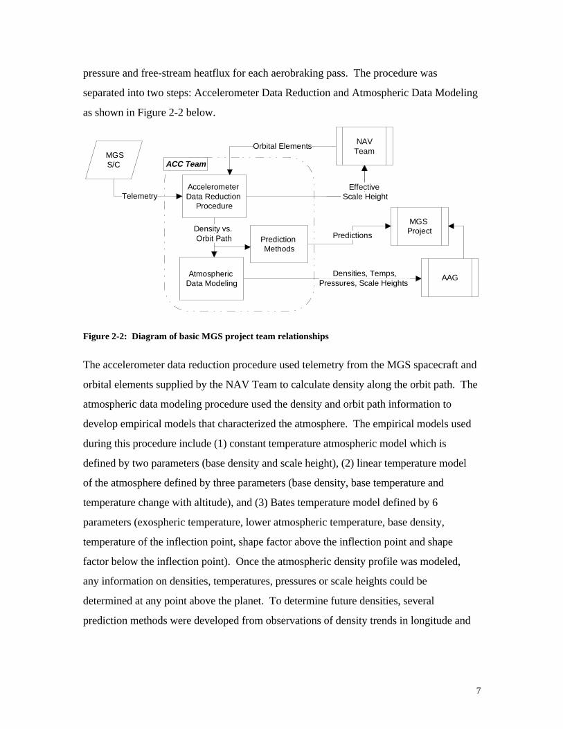
pressure and free-stream heatflux for each aerobraking pass. The procedure was

separated into two steps: Accelerometer Data Reduction and Atmospheric Data Modeling

as shown in Figure 2-2 below.

MGS S/C

NAV Team

Atmospheric Data Modeling

Telemetry

Orbital Elements

Effective Scale Height

Density vs. Orbit Path

AAG

MGS Project

ACC Team

Densities, Temps, Pressures, Scale Heights

PredictionsPrediction Methods

Accelerometer Data Reduction

Procedure

Figure 2-2: Diagram of basic MGS project team relationships

The accelerometer data reduction procedure used telemetry from the MGS spacecraft and

orbital elements supplied by the NAV Team to calculate density along the orbit path. The

atmospheric data modeling procedure used the density and orbit path information to

develop empirical models that characterized the atmosphere. The empirical models used

during this procedure include (1) constant temperature atmospheric model which is

defined by two parameters (base density and scale height), (2) linear temperature model

of the atmosphere defined by three parameters (base density, base temperature and

temperature change with altitude), and (3) Bates temperature model defined by 6

parameters (exospheric temperature, lower atmospheric temperature, base density,

temperature of the inflection point, shape factor above the inflection point and shape

factor below the inflection point). Once the atmospheric density profile was modeled,

any information on densities, temperatures, pressures or scale heights could be

determined at any point above the planet. To determine future densities, several

prediction methods were developed from observations of density trends in longitude and

8

latitude. This process culminated in a “quick-look” report distributed to all MGS project

teams. A typical quick-look report is described in Appendix A.

This paper describes in detail the methods used in the accelerometer data reduction

procedure as well as several prediction methods. The methods used in the atmospheric

data modeling procedure are not presented in this paper but are available in the paper by

Wilkerson [Wilkerson, B., “Upper Atmospheric Modeling for Mars Global Surveyor

Aerobraking Using Least Squared Processes,” Graduate Research Paper for George

Washington University, 1998. Available from author].

2.5 Description of Panel Malfunction

On November 6, 1996, MGS spacecraft telemetry indicated that the solar array on

the spacecraft -Y axis (SAM) failed to deploy into the fully extended position. To remedy

the failed deployment, the spacecraft was oriented such that aerodynamic forces would

extend the SAM during aerobraking passes at Mars. Early aerobraking passes showed the

SAM position moving closer to full extension. However, on pass 15 the MGS spacecraft

unexpectedly entered a high density region of the Martian atmosphere forcing the panel to

deflect past full extension by approximately 17 degrees based on sun sensor

measurements.

Following several aerobraking orbits at higher altitudes, aerobraking was stopped

altogether and an extensive testing program was initiated to determine the cause of the

over-extension and to evaluate the risk of continued aerobraking. After 25 days, it was

decided that the most likely scenario was that a crack had developed in the facesheet of

the SAM yoke. This crack, thought to be due to the initial deployment malfunction, was

apparently located on the compression facesheet where the thickness of the facesheet was

reduced. This theory was developed using spacecraft data and ground test data from a

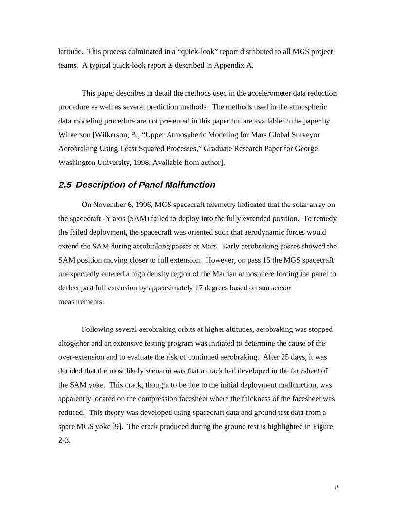
spare MGS yoke [9]. The crack produced during the ground test is highlighted in Figure

2-3.

9

YOKE CRACK LINE

Figure 2-3: Spare yoke with suspected failure mode

Assuming the integrity of the cracked yoke would not degrade under smaller forces,

aerobraking resumed at altitudes with lower dynamic pressures.

The analysis of accelerometer data had to consider the malfunction of the SAM

panel. The SAM panel, under the force of the atmosphere, deflected several degrees

during each aerobraking pass. The panel was also vibrating during each pass. Methods

were developed to compensate for both the deflection and the vibration.

10

3. Analysis of Acceleration Data

The aerodynamic force relationship forms the main equation for determining

density using data from an onboard accelerometer. For MGS, the z-accelerometer was

the primary data source used to measure the acceleration due to aerodynamic forces. The

equation that describes the density as a function of the acceleration due to aerodynamic

forces in the z-direction is

ρ =2

2

m a

v C AZ

Z (3-1)

In this equation, ρ is the atmospheric density, aZ is the acceleration of the spacecraft in the

spacecraft z-direction due to aerodynamic forces, v is the velocity of the spacecraft with

respect to the atmosphere, and m/CZA is the spacecraft ballistic coefficient. The ballistic

coefficient consists of the force coefficient in the spacecraft z-direction, the spacecraft

mass, and the spacecraft reference area. Methods developed to determine the

acceleration, the spacecraft velocity and the ballistic coefficient are discussed in the

sections below.

3.1 Development of the Acceleration Term

To determine the acceleration due to aerodynamic forces, all non-aerodynamic

effects must be removed from the acceleration measured by on-board accelerometers. The

measured acceleration signal can be written as

a a a a a a a ameasured aero gravgrad solar bias angular thruster vibration= + + + + + + (3-2)

The terms on the right hand side of Equation 3-2 represent the acceleration due to

aerodynamic forces, the gravity gradient acceleration, the acceleration due to solar

pressure, the instrument bias, the acceleration due to angular motion of the spacecraft, the

11

acceleration produced during thruster activity, and the acceleration due to vibration of the

damaged solar array. Each of these terms are described in more detail in Sections 3.1.1

through 3.1.7.

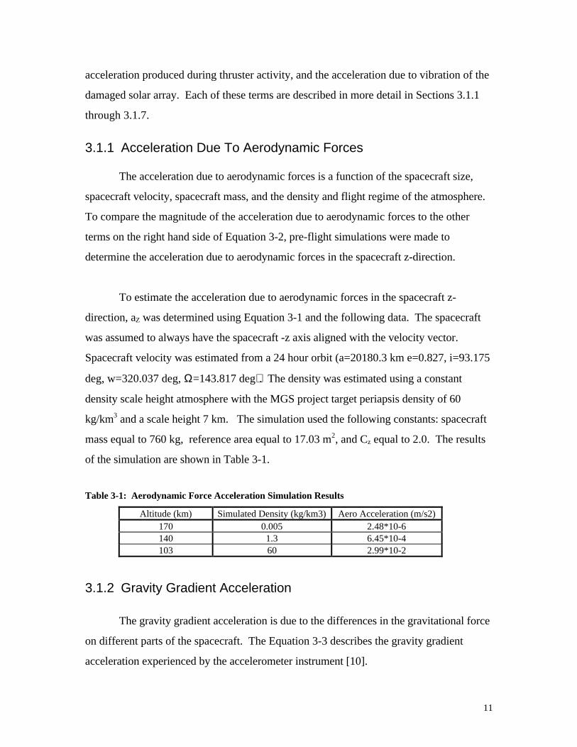
3.1.1 Acceleration Due To Aerodynamic Forces

The acceleration due to aerodynamic forces is a function of the spacecraft size,

spacecraft velocity, spacecraft mass, and the density and flight regime of the atmosphere.

To compare the magnitude of the acceleration due to aerodynamic forces to the other

terms on the right hand side of Equation 3-2, pre-flight simulations were made to

determine the acceleration due to aerodynamic forces in the spacecraft z-direction.

To estimate the acceleration due to aerodynamic forces in the spacecraft z-

direction, aZ was determined using Equation 3-1 and the following data. The spacecraft

was assumed to always have the spacecraft -z axis aligned with the velocity vector.

Spacecraft velocity was estimated from a 24 hour orbit (a=20180.3 km e=0.827, i=93.175

deg, w=320.037 deg, Ω=143.817 deg). The density was estimated using a constant

density scale height atmosphere with the MGS project target periapsis density of 60

kg/km3 and a scale height 7 km. The simulation used the following constants: spacecraft

mass equal to 760 kg, reference area equal to 17.03 m2, and Cz equal to 2.0. The results

of the simulation are shown in Table 3-1.

Table 3-1: Aerodynamic Force Acceleration Simulation Results

Altitude (km) Simulated Density (kg/km3) Aero Acceleration (m/s2)170 0.005 2.48*10-6140 1.3 6.45*10-4103 60 2.99*10-2

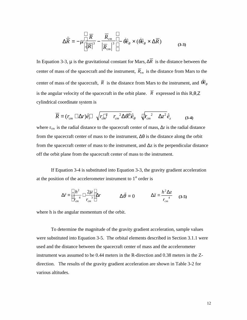
3.1.2 Gravity Gradient Acceleration

The gravity gradient acceleration is due to the differences in the gravitational force

on different parts of the spacecraft. The Equation 3-3 describes the gravity gradient

acceleration experienced by the accelerometer instrument [10].

12

∆ ∆ ( )RR

R

R

Re e R

cm

cm

= − −

− × ×µ θ θθ θ3 3 (3-3)

In Equation 3-3, µ is the gravitational constant for Mars,∆R is the distance between the

center of mass of the spacecraft and the instrument, Rcm is the distance from Mars to the

center of mass of the spacecraft, R is the distance from Mars to the instrument, and θ θe

is the angular velocity of the spacecraft in the orbit plane. R expressed in this R,θ,Ζ

cylindrical coordinate system is

R r r e r r e r z ecm r cm cm cm z= + + + + +( ) ∆ ∆ ∆2 2 2 2 2θ θ (3-4)

where rcm is the radial distance to the spacecraft center of mass, ∆r is the radial distance

from the spacecraft center of mass to the instrument, ∆θ is the distance along the orbit

from the spacecraft center of mass to the instrument, and ∆z is the perpendicular distance

off the orbit plane from the spacecraft center of mass to the instrument.

If Equation 3-4 is substituted into Equation 3-3, the gravity gradient acceleration

at the position of the accelerometer instrument to 1st order is

∆ ∆rh

r rr

cm cm

= +

2

4 3

2µ ∆ θ = 0 ∆

∆z

h z

rcm

=2

4 (3-5)

where h is the angular momentum of the orbit.

To determine the magnitude of the gravity gradient acceleration, sample values

were substituted into Equation 3-5. The orbital elements described in Section 3.1.1 were

used and the distance between the spacecraft center of mass and the accelerometer

instrument was assumed to be 0.44 meters in the R-direction and 0.38 meters in the Z-

direction. The results of the gravity gradient acceleration are shown in Table 3-2 for

various altitudes.

13

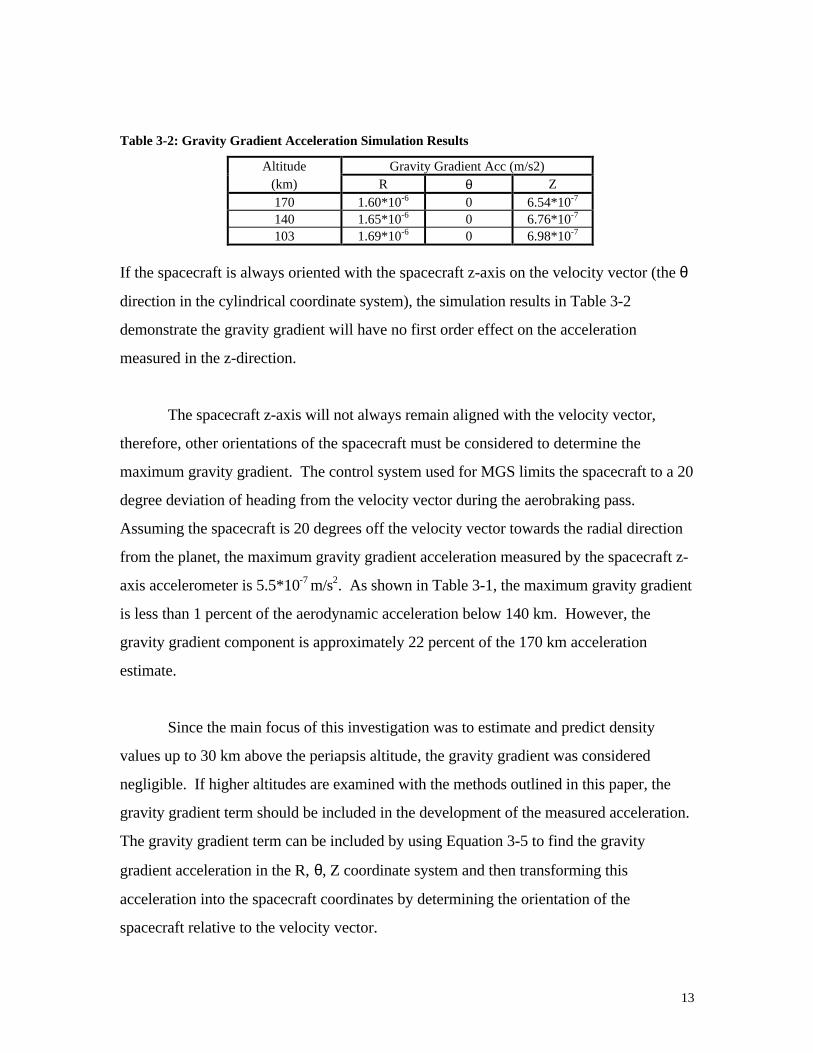
Table 3-2: Gravity Gradient Acceleration Simulation Results

Altitude Gravity Gradient Acc (m/s2)(km) R θ Z170 1.60*10-6 0 6.54*10-7

140 1.65*10-6 0 6.76*10-7

103 1.69*10-6 0 6.98*10-7

If the spacecraft is always oriented with the spacecraft z-axis on the velocity vector (the θ

direction in the cylindrical coordinate system), the simulation results in Table 3-2

demonstrate the gravity gradient will have no first order effect on the acceleration

measured in the z-direction.

The spacecraft z-axis will not always remain aligned with the velocity vector,

therefore, other orientations of the spacecraft must be considered to determine the

maximum gravity gradient. The control system used for MGS limits the spacecraft to a 20

degree deviation of heading from the velocity vector during the aerobraking pass.

Assuming the spacecraft is 20 degrees off the velocity vector towards the radial direction

from the planet, the maximum gravity gradient acceleration measured by the spacecraft z-

axis accelerometer is 5.5*10-7 m/s2. As shown in Table 3-1, the maximum gravity gradient

is less than 1 percent of the aerodynamic acceleration below 140 km. However, the

gravity gradient component is approximately 22 percent of the 170 km acceleration

estimate.

Since the main focus of this investigation was to estimate and predict density

values up to 30 km above the periapsis altitude, the gravity gradient was considered

negligible. If higher altitudes are examined with the methods outlined in this paper, the

gravity gradient term should be included in the development of the measured acceleration.

The gravity gradient term can be included by using Equation 3-5 to find the gravity

gradient acceleration in the R, θ, Z coordinate system and then transforming this

acceleration into the spacecraft coordinates by determining the orientation of the

spacecraft relative to the velocity vector.

14

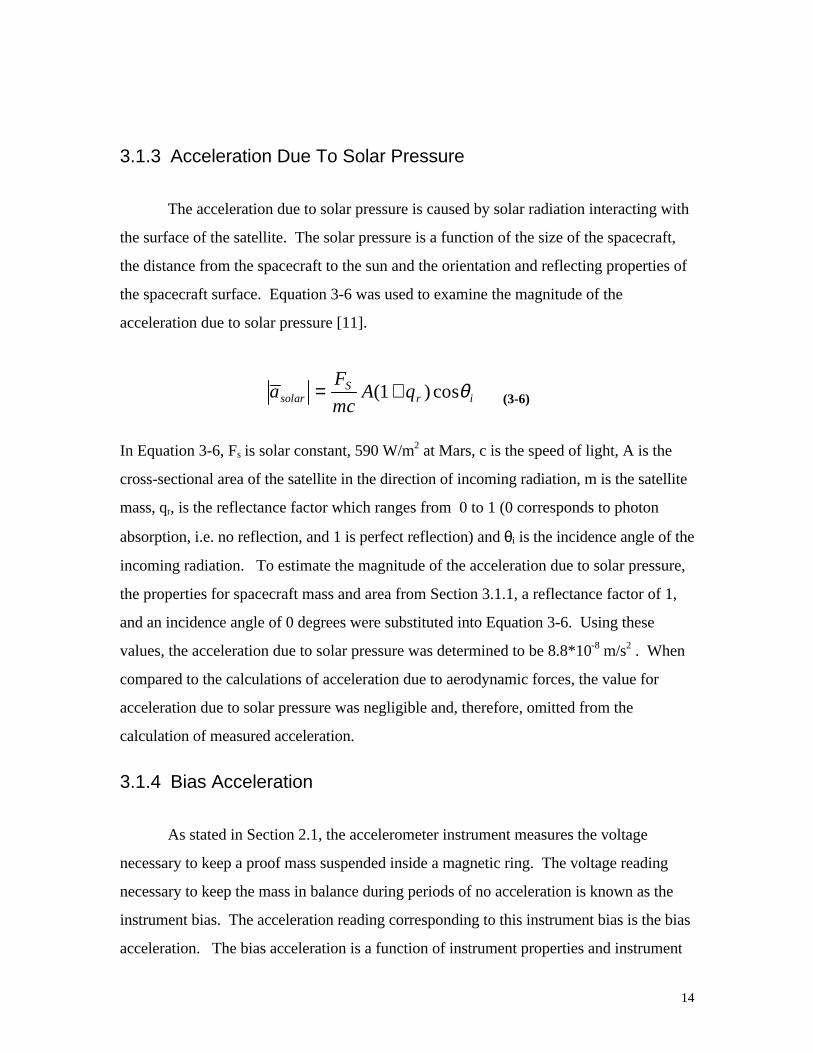
3.1.3 Acceleration Due To Solar Pressure

The acceleration due to solar pressure is caused by solar radiation interacting with

the surface of the satellite. The solar pressure is a function of the size of the spacecraft,

the distance from the spacecraft to the sun and the orientation and reflecting properties of

the spacecraft surface. Equation 3-6 was used to examine the magnitude of the

acceleration due to solar pressure [11].

aF

mcA qsolar

Sr i= +( ) cos1 θ (3-6)

In Equation 3-6, Fs is solar constant, 590 W/m2 at Mars, c is the speed of light, A is the

cross-sectional area of the satellite in the direction of incoming radiation, m is the satellite

mass, qr, is the reflectance factor which ranges from 0 to 1 (0 corresponds to photon

absorption, i.e. no reflection, and 1 is perfect reflection) and θi is the incidence angle of the

incoming radiation. To estimate the magnitude of the acceleration due to solar pressure,

the properties for spacecraft mass and area from Section 3.1.1, a reflectance factor of 1,

and an incidence angle of 0 degrees were substituted into Equation 3-6. Using these

values, the acceleration due to solar pressure was determined to be 8.8*10-8 m/s2 . When

compared to the calculations of acceleration due to aerodynamic forces, the value for

acceleration due to solar pressure was negligible and, therefore, omitted from the

calculation of measured acceleration.

3.1.4 Bias Acceleration

As stated in Section 2.1, the accelerometer instrument measures the voltage

necessary to keep a proof mass suspended inside a magnetic ring. The voltage reading

necessary to keep the mass in balance during periods of no acceleration is known as the

instrument bias. The acceleration reading corresponding to this instrument bias is the bias

acceleration. The bias acceleration is a function of instrument properties and instrument

15

temperature. To determine the acceleration bias, the instrument must be continually

checked and the surrounding temperature continuously monitored such that drift, i.e.

change in the bias value as a function of time, can be determined.

For the MGS mission, bias was determined by monitoring the accelerometer

instrument during periods before and after entering the atmosphere. The bias acceleration

was then estimated over the entire pass by averaging the data from the pre- and post-

atmospheric entry periods. The pre- and post-atmospheric periods were defined by

instrument on and off times and an altitude limit of the atmosphere. For the MGS mission,

the altitude limit was set by examining the acceleration profile and selecting an altitude

well above the first indications of accelerations due to the atmosphere, typically 200 km.

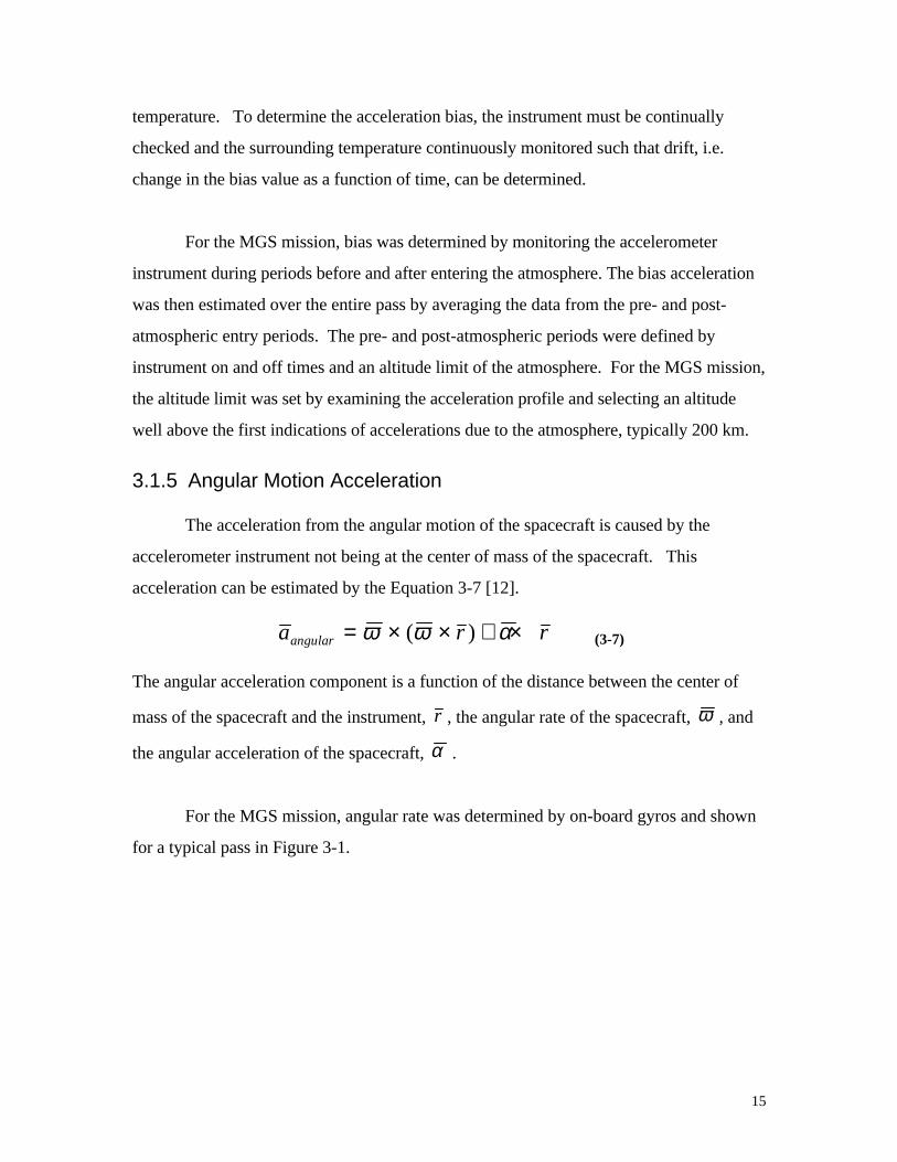
3.1.5 Angular Motion Acceleration

The acceleration from the angular motion of the spacecraft is caused by the

accelerometer instrument not being at the center of mass of the spacecraft. This

acceleration can be estimated by the Equation 3-7 [12].

a r rangular = × × + ×ω ω α( ) (3-7)

The angular acceleration component is a function of the distance between the center of

mass of the spacecraft and the instrument, r , the angular rate of the spacecraft, ω , and

the angular acceleration of the spacecraft, α .

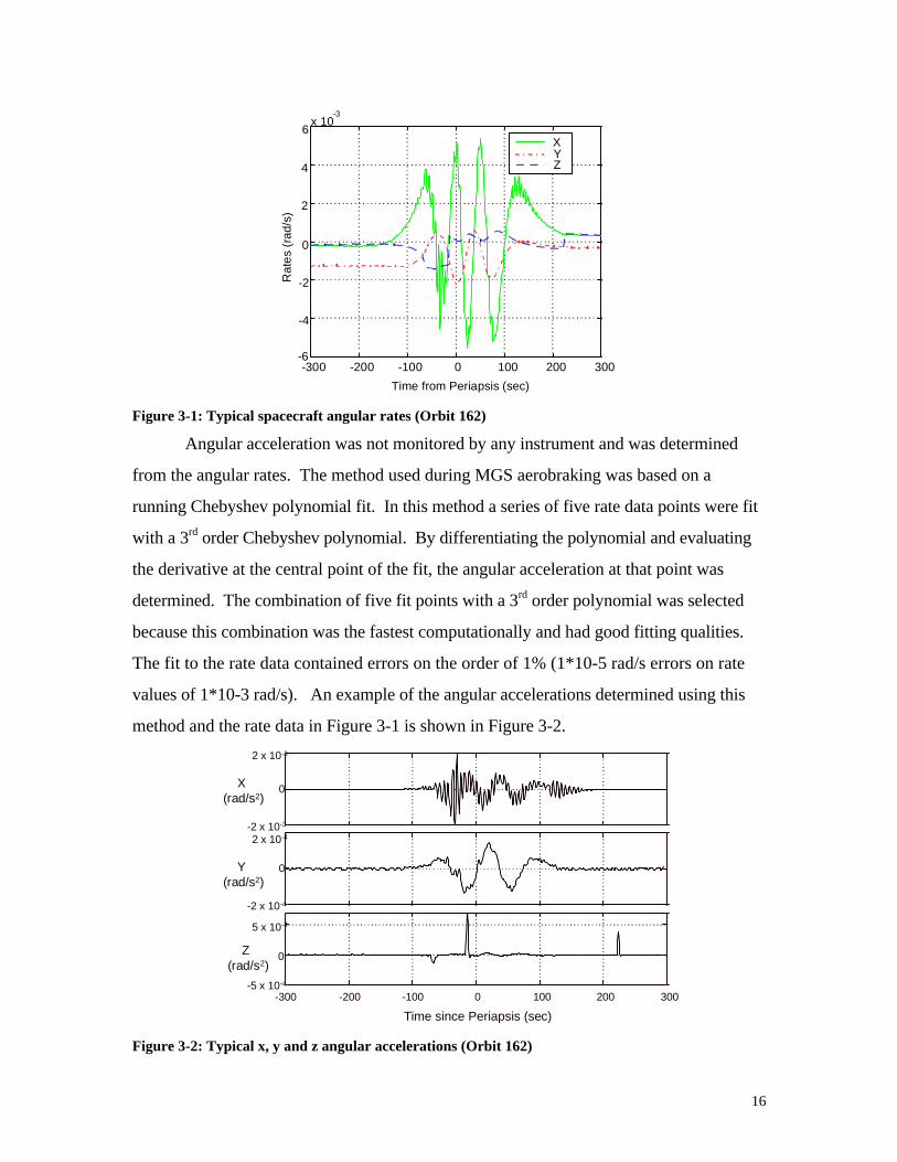
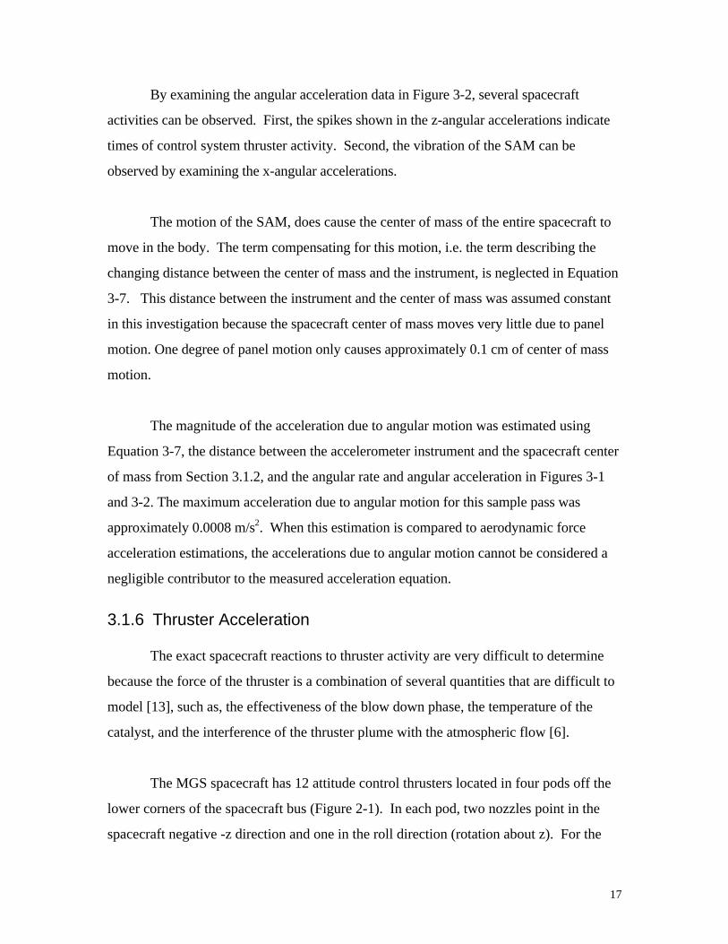
For the MGS mission, angular rate was determined by on-board gyros and shown

for a typical pass in Figure 3-1.

16

-300 -200 -100 0 100 200 300-6

-4

-2

0

2

4

6x 10

-3

Time from Periapsis (sec)

Rat

es

(rad

/s)

XYZ

Figure 3-1: Typical spacecraft angular rates (Orbit 162)

Angular acceleration was not monitored by any instrument and was determined

from the angular rates. The method used during MGS aerobraking was based on a

running Chebyshev polynomial fit. In this method a series of five rate data points were fit

with a 3rd order Chebyshev polynomial. By differentiating the polynomial and evaluating

the derivative at the central point of the fit, the angular acceleration at that point was

determined. The combination of five fit points with a 3rd order polynomial was selected

because this combination was the fastest computationally and had good fitting qualities.

The fit to the rate data contained errors on the order of 1% (1*10-5 rad/s errors on rate

values of 1*10-3 rad/s). An example of the angular accelerations determined using this

method and the rate data in Figure 3-1 is shown in Figure 3-2.

0

-300 -200 -100 0 100 200 300

0

Time since Periapsis (sec)

0

2 x 10-3

-2 x 10-3

2 x 10-4

-2 x 10-4

Z (rad/s2)

Y (rad/s2)

X (rad/s2)

5 x 10-4

-5 x 10-4

Figure 3-2: Typical x, y and z angular accelerations (Orbit 162)

17

By examining the angular acceleration data in Figure 3-2, several spacecraft

activities can be observed. First, the spikes shown in the z-angular accelerations indicate

times of control system thruster activity. Second, the vibration of the SAM can be

observed by examining the x-angular accelerations.

The motion of the SAM, does cause the center of mass of the entire spacecraft to

move in the body. The term compensating for this motion, i.e. the term describing the

changing distance between the center of mass and the instrument, is neglected in Equation

3-7. This distance between the instrument and the center of mass was assumed constant

in this investigation because the spacecraft center of mass moves very little due to panel

motion. One degree of panel motion only causes approximately 0.1 cm of center of mass

motion.

The magnitude of the acceleration due to angular motion was estimated using

Equation 3-7, the distance between the accelerometer instrument and the spacecraft center

of mass from Section 3.1.2, and the angular rate and angular acceleration in Figures 3-1

and 3-2. The maximum acceleration due to angular motion for this sample pass was

approximately 0.0008 m/s2. When this estimation is compared to aerodynamic force

acceleration estimations, the accelerations due to angular motion cannot be considered a

negligible contributor to the measured acceleration equation.

3.1.6 Thruster Acceleration

The exact spacecraft reactions to thruster activity are very difficult to determine

because the force of the thruster is a combination of several quantities that are difficult to

model [13], such as, the effectiveness of the blow down phase, the temperature of the

catalyst, and the interference of the thruster plume with the atmospheric flow [6].

The MGS spacecraft has 12 attitude control thrusters located in four pods off the

lower corners of the spacecraft bus (Figure 2-1). In each pod, two nozzles point in the

spacecraft negative -z direction and one in the roll direction (rotation about z). For the

18

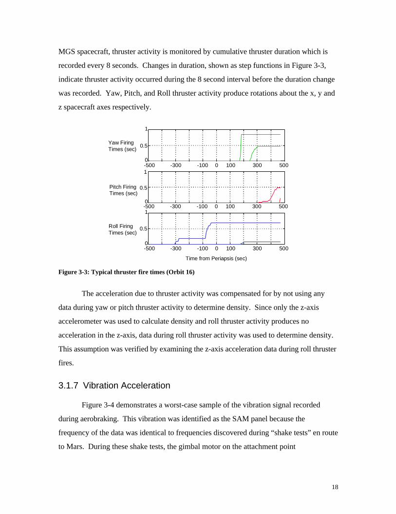
MGS spacecraft, thruster activity is monitored by cumulative thruster duration which is

recorded every 8 seconds. Changes in duration, shown as step functions in Figure 3-3,

indicate thruster activity occurred during the 8 second interval before the duration change

was recorded. Yaw, Pitch, and Roll thruster activity produce rotations about the x, y and

z spacecraft axes respectively.

-500 -300 -100 0 100 300 5000

0.5

1

0

0.5

1

0

1

Roll FiringTimes (sec)

Pitch FiringTimes (sec)

Yaw FiringTimes (sec)

Time from Periapsis (sec)

0.5

-500 -300 -100 0 100 300 500

-500 -300 -100 0 100 300 500

Figure 3-3: Typical thruster fire times (Orbit 16)

The acceleration due to thruster activity was compensated for by not using any

data during yaw or pitch thruster activity to determine density. Since only the z-axis

accelerometer was used to calculate density and roll thruster activity produces no

acceleration in the z-axis, data during roll thruster activity was used to determine density.

This assumption was verified by examining the z-axis acceleration data during roll thruster

fires.

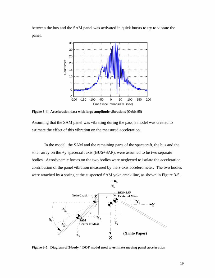
3.1.7 Vibration Acceleration

Figure 3-4 demonstrates a worst-case sample of the vibration signal recorded

during aerobraking. This vibration was identified as the SAM panel because the

frequency of the data was identical to frequencies discovered during “shake tests” en route

to Mars. During these shake tests, the gimbal motor on the attachment point

19

between the bus and the SAM panel was activated in quick bursts to try to vibrate the

panel.

Cou

nts/

sec

-200 -150 -100 -50 0 50 100 150 200

Time Since Periapsis 95 (sec)

-5

0

5

10

15

20

25

30

35

Figure 3-4: Acceleration data with large amplitude vibrations (Orbit 95)

Assuming that the SAM panel was vibrating during the pass, a model was created to

estimate the effect of this vibration on the measured acceleration.

In the model, the SAM and the remaining parts of the spacecraft, the bus and the

solar array on the +y spacecraft axis (BUS+SAP), were assumed to be two separate

bodies. Aerodynamic forces on the two bodies were neglected to isolate the acceleration

contribution of the panel vibration measured by the z-axis accelerometer. The two bodies

were attached by a spring at the suspected SAM yoke crack line, as shown in Figure 3-5.

Y

Z

Z1

Z2

Y1

Y2

θ0

θδ

θ1

Yoke CrackBUS+SAP Center of Mass

SAM Center of Mass

ab

θ2

(X into Paper)

L

Figure 3-5: Diagram of 2-body 4 DOF model used to estimate moving panel acceleration

20

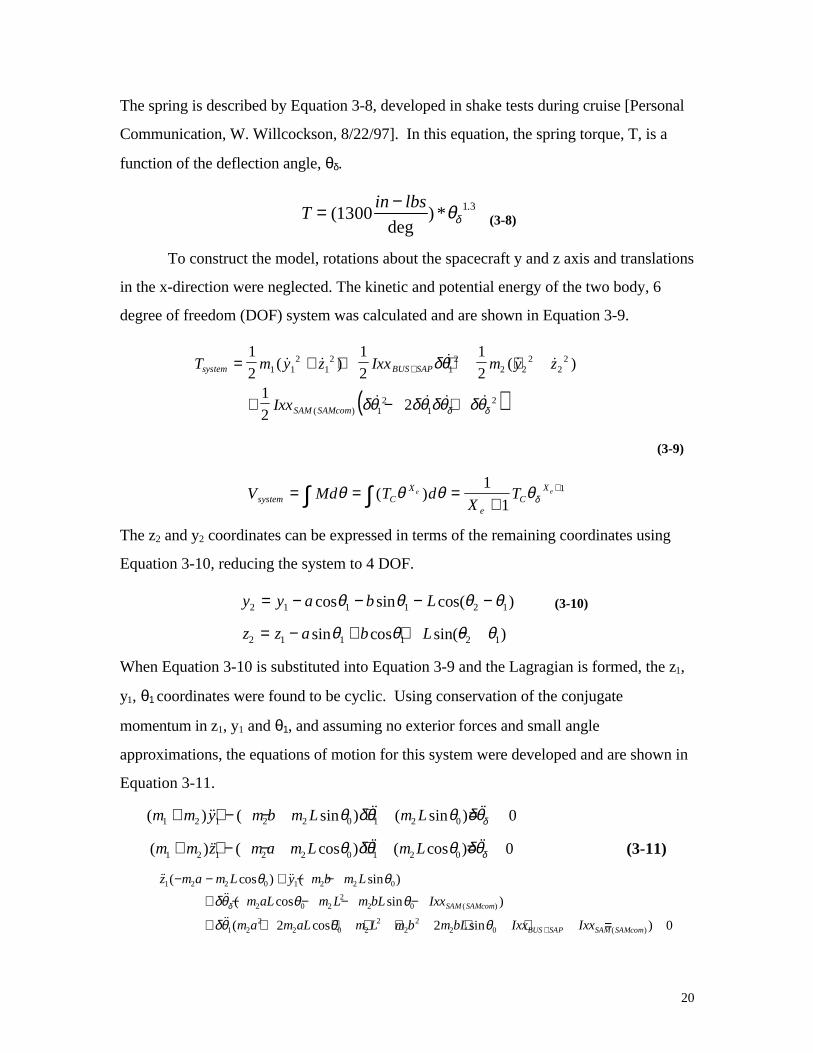
The spring is described by Equation 3-8, developed in shake tests during cruise [Personal

Communication, W. Willcockson, 8/22/97]. In this equation, the spring torque, T, is a

function of the deflection angle, θδ.

Tin lbs= −

(deg

) * .1300 1 3θδ (3-8)

To construct the model, rotations about the spacecraft y and z axis and translations

in the x-direction were neglected. The kinetic and potential energy of the two body, 6

degree of freedom (DOF) system was calculated and are shown in Equation 3-9.

( )T m y z Ixx m y z

Ixx

system BUS SAP

SAM SAMcom

= + + + +

+ − +

+

1

2

1

2

1

21

22

1 12

12

12

2 22

22

12

12

( ) ( )

( )

δθ

δθ δθ δθ δθδ δ

(3-9)

V Md T dX

Tsystem CX

eC

Xe e= = =+∫ ∫ +θ θ θ θδ( )

1

11

The z2 and y2 coordinates can be expressed in terms of the remaining coordinates using

Equation 3-10, reducing the system to 4 DOF.

y y a b L2 1 1 1 2 1= − − − −cos sin cos( )θ θ θ θ (3-10)

z z a b L2 1 1 1 2 1= − + + −sin cos sin( )θ θ θ θ

When Equation 3-10 is substituted into Equation 3-9 and the Lagragian is formed, the z1,

y1, θ1 coordinates were found to be cyclic. Using conservation of the conjugate

momentum in z1, y1 and θ1, and assuming no exterior forces and small angle

approximations, the equations of motion for this system were developed and are shown in

Equation 3-11.

( ) ( sin ) ( sin ) m m y m b m L m L1 2 1 2 2 0 1 2 0 0+ + − − + =θ δθ θ δθδ

( ) ( cos ) ( cos ) m m z m a m L m L1 2 1 2 2 0 1 2 0 0+ + − − + =θ δθ θ δθδ (3-11)

( cos ) ( sin ) ( cos sin )

( cos sin )

( )

( )

z m a m L y m b m L

m aL m L m bL Ixx

m a m aL m L m b m bL Ixx Ixx

SAM SAMcom

BUS SAP SAM SAMcom

1 2 2 0 1 2 2 0

2 0 22

2 0

1 22

2 0 22

22

2 02 2 0

− − + − −

+ − − − −

+ + + + + + + =+

θ θ

δθ θ θ

δθ θ θδ

21

In this problemθ1 is the angular acceleration in the spacecraft x-direction, which was

determined from onboard gyro data as shown in Section 3.1.5. Equation 3-11 is solved for

z1 , the acceleration of the BUS+SAP center of mass due to the motion of the SAM panel. A

complete derivation of the system is shown in Appendix B.

An important note is that by assuming the BUS+SAP and SAM are separate

masses, the gyros located on the BUS are only monitoring the BUS+SAP body.

Therefore, to identify the acceleration from spacecraft angular motion described in Section

3.1.5, the center of mass of the BUS+SAP body must be used instead of the entire

spacecraft center of mass to determine the distance, r, in the angular motion equation,

Equation 3-7. This distance, r, is assumed constant because the BUS+SAP body is

considered rigid.

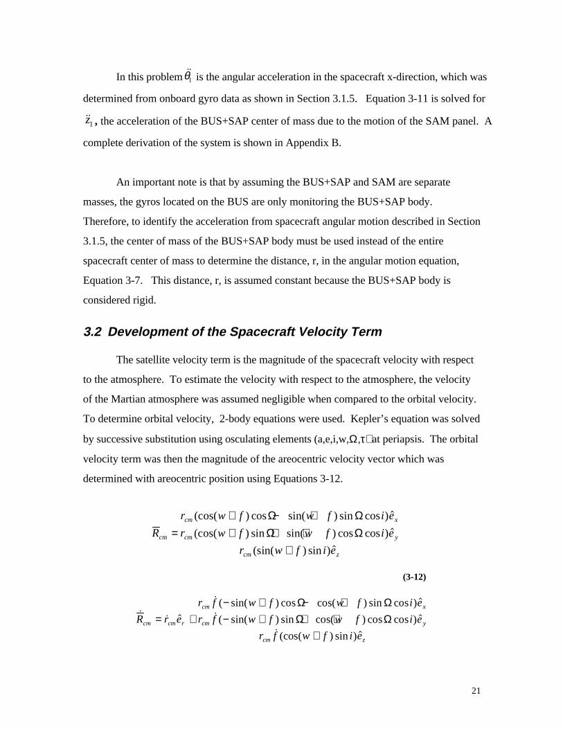
3.2 Development of the Spacecraft Velocity Term

The satellite velocity term is the magnitude of the spacecraft velocity with respect

to the atmosphere. To estimate the velocity with respect to the atmosphere, the velocity

of the Martian atmosphere was assumed negligible when compared to the orbital velocity.

To determine orbital velocity, 2-body equations were used. Kepler’s equation was solved

by successive substitution using osculating elements (a,e,i,w,Ω,τ) at periapsis. The orbital

velocity term was then the magnitude of the areocentric velocity vector which was

determined with areocentric position using Equations 3-12.

R

r w f w f i e

r w f w f i e

r w f i ecm

cm x

cm y

cm z

=+ − ++ + +

+

(cos( ) cos sin( ) sin cos )

(cos( ) sin sin( ) cos cos )

(sin( ) sin )

Ω ΩΩ Ω

(3-12)

( sin( ) cos cos( ) sin cos ) ( sin( ) sin cos( ) cos cos )

(cos( ) sin )

R r e

r f w f w f i e

r f w f w f i e

r f w f i ecm cm r

cm x

cm y

cm z

= +− + − +− + + +

+

Ω ΩΩ Ω

22

In Equation 3-12, rcm is the radial position, w is the argument of periapsis, f is the true

anomaly, Ω is the longitude of the ascending node, and i is the inclination.

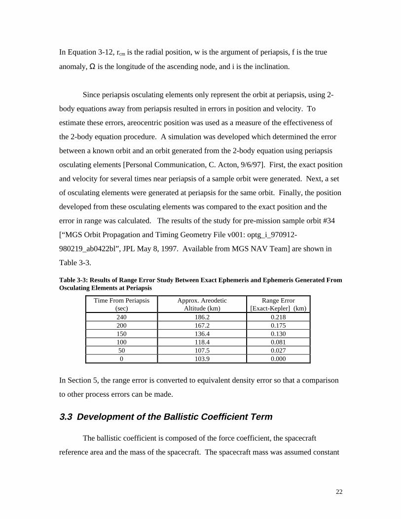
Since periapsis osculating elements only represent the orbit at periapsis, using 2-

body equations away from periapsis resulted in errors in position and velocity. To

estimate these errors, areocentric position was used as a measure of the effectiveness of

the 2-body equation procedure. A simulation was developed which determined the error

between a known orbit and an orbit generated from the 2-body equation using periapsis

osculating elements [Personal Communication, C. Acton, 9/6/97]. First, the exact position

and velocity for several times near periapsis of a sample orbit were generated. Next, a set

of osculating elements were generated at periapsis for the same orbit. Finally, the position

developed from these osculating elements was compared to the exact position and the

error in range was calculated. The results of the study for pre-mission sample orbit #34

[“MGS Orbit Propagation and Timing Geometry File v001: optg_i_970912-

980219_ab0422bl”, JPL May 8, 1997. Available from MGS NAV Team] are shown in

Table 3-3.

Table 3-3: Results of Range Error Study Between Exact Ephemeris and Ephemeris Generated FromOsculating Elements at Periapsis

Time From Periapsis(sec)

Approx. AreodeticAltitude (km)

Range Error[Exact-Kepler] (km)

240 186.2 0.218200 167.2 0.175150 136.4 0.130100 118.4 0.08150 107.5 0.0270 103.9 0.000

In Section 5, the range error is converted to equivalent density error so that a comparison

to other process errors can be made.

3.3 Development of the Ballistic Coefficient Term

The ballistic coefficient is composed of the force coefficient, the spacecraft

reference area and the mass of the spacecraft. The spacecraft mass was assumed constant

23

during an aerobraking pass because fuel usage by control system thrusters was small

(<< 1kg) compared to the total spacecraft mass (approx. 760 kg). The spacecraft

reference area was calculated as the cross-sectional area seen by the flow when the

spacecraft is in the aerobraking configuration with the spacecraft -z axis aligned with the

velocity vector. The force coefficient was determined by developing an aerodynamic

database of force coefficients and interpolating the value of the coefficient by knowing the

spacecraft orientation, and by estimating the panel deflection angle and the density of the

atmosphere. The following sections describe the development of the aerodynamic

database and the use of the database to determine force coefficients.

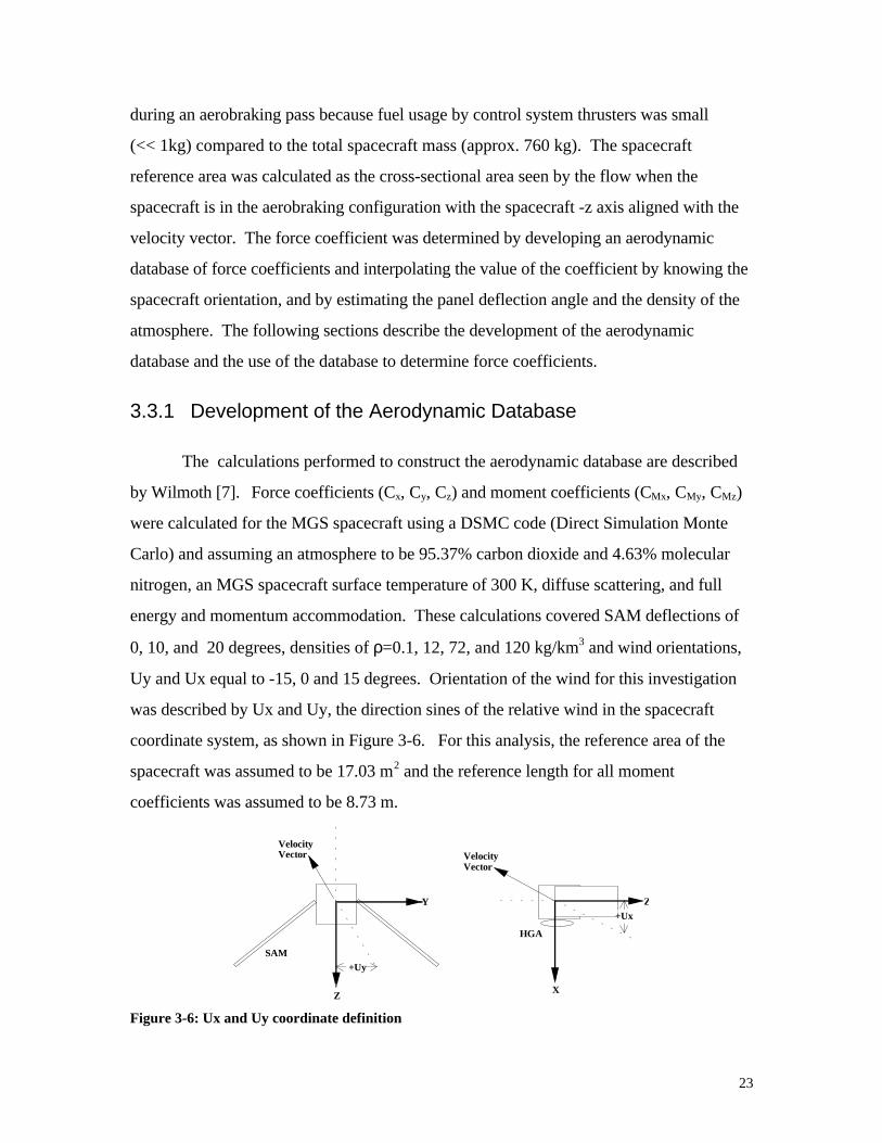
3.3.1 Development of the Aerodynamic Database

The calculations performed to construct the aerodynamic database are described

by Wilmoth [7]. Force coefficients (Cx, Cy, Cz) and moment coefficients (CMx, CMy, CMz)

were calculated for the MGS spacecraft using a DSMC code (Direct Simulation Monte

Carlo) and assuming an atmosphere to be 95.37% carbon dioxide and 4.63% molecular

nitrogen, an MGS spacecraft surface temperature of 300 K, diffuse scattering, and full

energy and momentum accommodation. These calculations covered SAM deflections of

0, 10, and 20 degrees, densities of ρ=0.1, 12, 72, and 120 kg/km3 and wind orientations,

Uy and Ux equal to -15, 0 and 15 degrees. Orientation of the wind for this investigation

was described by Ux and Uy, the direction sines of the relative wind in the spacecraft

coordinate system, as shown in Figure 3-6. For this analysis, the reference area of the

spacecraft was assumed to be 17.03 m2 and the reference length for all moment

coefficients was assumed to be 8.73 m.

Z

Y

+Uy

Z

X

+Ux

VelocityVector Velocity

Vector

SAM

HGA

Figure 3-6: Ux and Uy coordinate definition

24

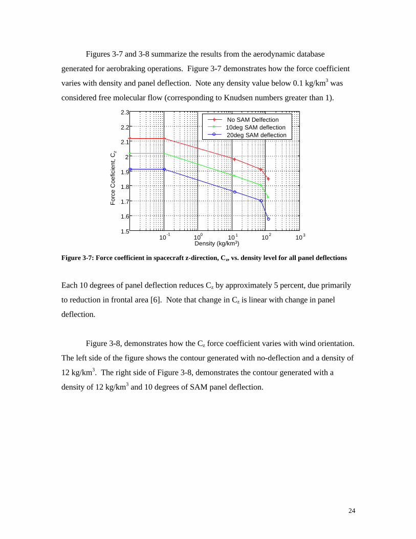
Figures 3-7 and 3-8 summarize the results from the aerodynamic database

generated for aerobraking operations. Figure 3-7 demonstrates how the force coefficient

varies with density and panel deflection. Note any density value below 0.1 kg/km3 was

considered free molecular flow (corresponding to Knudsen numbers greater than 1).

10-1

100

10 1 102

10 31.5

1.6

1.7

1.8

1.9

2

2.1

2.2

2.3

Density (kg/km3)

For

ce C

oefic

ient

, Cz

No SAM Delfection 10deg SAM deflection20deg SAM deflection

Figure 3-7: Force coefficient in spacecraft z-direction, Cz, vs. density level for all panel deflections

Each 10 degrees of panel deflection reduces Cz by approximately 5 percent, due primarily

to reduction in frontal area [6]. Note that change in Cz is linear with change in panel

deflection.

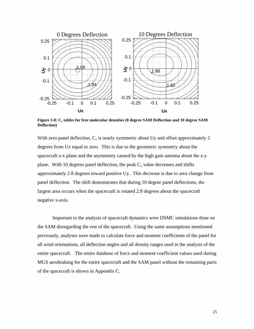
Figure 3-8, demonstrates how the Cz force coefficient varies with wind orientation.

The left side of the figure shows the contour generated with no-deflection and a density of

12 kg/km3. The right side of Figure 3-8, demonstrates the contour generated with a

density of 12 kg/km3 and 10 degrees of SAM panel deflection.

25

-0.25

Uy

-0.1

0

0.1

0.25

1.94

1.98

Ux

-0.25 -0.1 0 0.1 0.25

1.82

1.86

Ux

Uy

-0.25

-0.1

0

0.1

0.25

-0.25 -0.1 0 0.1 0.25

0 Degrees Deflection 10 Degrees Deflection

Figure 3-8: Cz tables for free molecular densities (0 degree SAM Deflection and 10 degree SAMDeflection)

With zero panel deflection, Cz is nearly symmetric about Uy and offset approximately 2

degrees from Ux equal to zero. This is due to the geometric symmetry about the

spacecraft z-x plane and the asymmetry caused by the high gain antenna about the z-y

plane. With 10 degrees panel deflection, the peak Cz value decreases and shifts

approximately 2.8 degrees toward positive Uy. This decrease is due to area change from

panel deflection. The shift demonstrates that during 10 degree panel deflections, the

largest area occurs when the spacecraft is rotated 2.8 degrees about the spacecraft

negative x-axis.

Important to the analysis of spacecraft dynamics were DSMC simulations done on

the SAM disregarding the rest of the spacecraft. Using the same assumptions mentioned

previously, analyses were made to calculate force and moment coefficients of the panel for

all wind orientations, all deflection angles and all density ranges used in the analysis of the

entire spacecraft. The entire database of force and moment coefficient values used during

MGS aerobraking for the entire spacecraft and the SAM panel without the remaining parts

of the spacecraft is shown in Appendix C.

26

3.3.2 Determining Force Coefficients

Force coefficients were determined by interpolation of the aerodynamic database.

Inputs to this interpolation were the orientation of the relative wind, density, and panel

position. Density and panel position were determined by the iterative scheme discussed in

Section 4.4.3. The orientation of the incoming wind was determined by combining the

orbital velocity and the atmospheric winds in the spacecraft centered system.

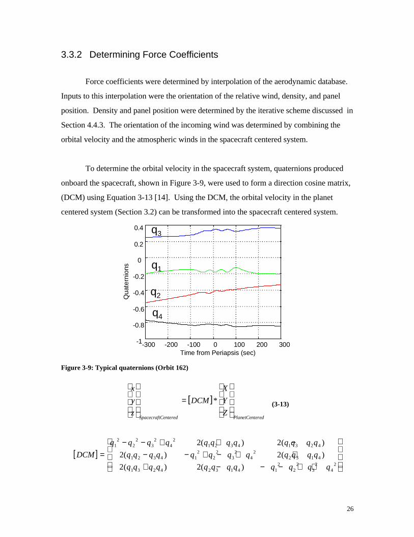
To determine the orbital velocity in the spacecraft system, quaternions produced

onboard the spacecraft, shown in Figure 3-9, were used to form a direction cosine matrix,

(DCM) using Equation 3-13 [14]. Using the DCM, the orbital velocity in the planet

centered system (Section 3.2) can be transformed into the spacecraft centered system.

-300 -200 -100 0 100 200 300-1

-0.8

-0.6

-0.4

-0.2

0

0.2

0.4

Time from Periapsis (sec)

Qua

tern

ions q1

q2

q3

q4

Figure 3-9: Typical quaternions (Orbit 162)

[ ]x

y

z

DCM

X

Y

ZSpacecraftCentered PlanetCentered

=

* (3-13)

[ ]DCM

q q q q q q q q q q q q

q q q q q q q q q q q q

q q q q q q q q q q q q

=− − + + −

− − + − + ++ − − − + +

12

22

32

42

1 2 3 4 1 3 2 4

1 2 3 4 12

22

32

42

2 3 1 4

1 3 2 4 2 3 1 4 12

22

32

42

2 2

2 2

2 2

( ) ( )

( ) ( )

( ) ( )

27

The atmospheric wind is modeled as the wind due to rigid rotation of the

atmosphere. The velocity of the atmospheric wind was calculated using Equation 3-14,

the rotation rate of the planet, L , and the spacecraft distance from the planet, Rcm .

v L RWIND cm= × (3-14)

This wind was then transformed with the same DCM created above into the spacecraft

centered system.

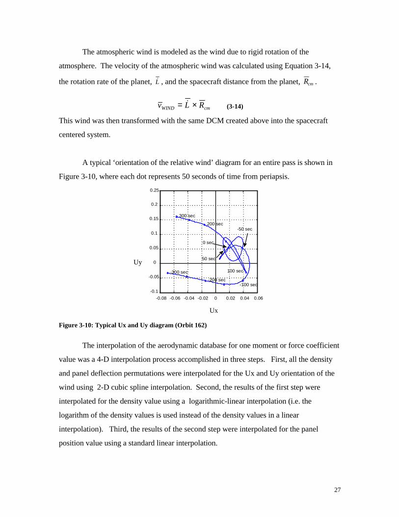
A typical ‘orientation of the relative wind’ diagram for an entire pass is shown in

Figure 3-10, where each dot represents 50 seconds of time from periapsis.

-0.08 -0.06 -0.04 -0.02 0 0.02 0.04 0.06

-0.1

-0.05

0

0.05

0.1

0.15

0.2

0.25

-200 sec

0 sec

100 sec

50 sec

300 sec

200 sec

-300 sec

-50 sec

-100 sec

Ux

Uy

Figure 3-10: Typical Ux and Uy diagram (Orbit 162)

The interpolation of the aerodynamic database for one moment or force coefficient

value was a 4-D interpolation process accomplished in three steps. First, all the density

and panel deflection permutations were interpolated for the Ux and Uy orientation of the

wind using 2-D cubic spline interpolation. Second, the results of the first step were

interpolated for the density value using a logarithmic-linear interpolation (i.e. the

logarithm of the density values is used instead of the density values in a linear

interpolation). Third, the results of the second step were interpolated for the panel

position value using a standard linear interpolation.

28

4. Operational Data Reduction Procedure

Section 4 will discuss the procedures and studies performed to create the

operational data reduction procedure used to determine densities from accelerometer data

during the 1st phase of aerobraking at Mars. First the operational scenario including

mission constraints and the operational accelerometer instrument is discussed. The

amount of accelerometer data necessary to perform the operational responsibilities is

determined. Next, the data reduction procedure is described using Section 3 methods

modified for the MGS operational scenario. Finally, several extra products of the data

reduction procedure as well as prediction methods are discussed.

4.1 Operational Constraints

To be effective during aerobraking operations, methods used to calculate density

have to be computed quickly and accurately over a range of altitudes. According to MGS

project constraints, all accelerometer data analysis must be completed within 2 hours of

receiving data. Since most of this time should be devoted to the analysis of density trends,

the procedure to calculate density for the entire orbit should be completed in one quarter

of the allowable time or 30 minutes. To fully understand the atmosphere, the calculation

of density must be accurate over a large range of altitudes. The methods were designed to

be accurate over an altitude range of 30 km above periapsis. This altitude range was

chosen to allow density to be calculated over approximately 4 scale heights.

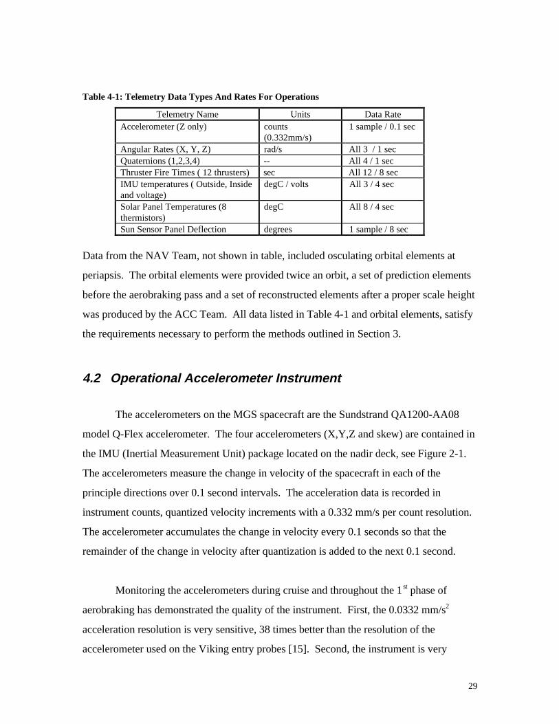
The data provided to perform the accelerometer data reduction process included

all values shown in Table 4-1. These data types were provided every aerobraking pass by

telemetry. Note accelerometer data rate for the first 15 aerobraking orbits was 10 samples

every 8 seconds. This data rate was increased to 1 sample every 0.1 seconds when

aerobraking resumed after the investigation of the panel over-extension.

29

Table 4-1: Telemetry Data Types And Rates For Operations

Telemetry Name Units Data RateAccelerometer (Z only) counts

(0.332mm/s) 1 sample / 0.1 sec

Angular Rates (X, Y, Z) rad/s All 3 / 1 secQuaternions (1,2,3,4) -- All 4 / 1 secThruster Fire Times ( 12 thrusters) sec All 12 / 8 secIMU temperatures ( Outside, Insideand voltage)

degC / volts All 3 / 4 sec

Solar Panel Temperatures (8thermistors)

degC All 8 / 4 sec

Sun Sensor Panel Deflection degrees 1 sample / 8 sec

Data from the NAV Team, not shown in table, included osculating orbital elements at

periapsis. The orbital elements were provided twice an orbit, a set of prediction elements

before the aerobraking pass and a set of reconstructed elements after a proper scale height

was produced by the ACC Team. All data listed in Table 4-1 and orbital elements, satisfy

the requirements necessary to perform the methods outlined in Section 3.

4.2 Operational Accelerometer Instrument

The accelerometers on the MGS spacecraft are the Sundstrand QA1200-AA08

model Q-Flex accelerometer. The four accelerometers (X,Y,Z and skew) are contained in

the IMU (Inertial Measurement Unit) package located on the nadir deck, see Figure 2-1.

The accelerometers measure the change in velocity of the spacecraft in each of the

principle directions over 0.1 second intervals. The acceleration data is recorded in

instrument counts, quantized velocity increments with a 0.332 mm/s per count resolution.

The accelerometer accumulates the change in velocity every 0.1 seconds so that the

remainder of the change in velocity after quantization is added to the next 0.1 second.

Monitoring the accelerometers during cruise and throughout the 1st phase of

aerobraking has demonstrated the quality of the instrument. First, the 0.0332 mm/s2

acceleration resolution is very sensitive, 38 times better than the resolution of the

accelerometer used on the Viking entry probes [15]. Second, the instrument is very

30

stable. During the travel to Mars, two separate measurements taken before trajectory

correction maneuvers (TCM), 8 months apart, resulted in a bias change of only 2%

(TCM-1 bias=5.62 +/- 0.12 counts/0.1 sec, TCM-2 bias=5.70 +/- 0.05 counts/0.1 sec).

During aerobraking, the bias remained at 5.66 +/- 0.005 counts/0.1 sec, varying only 0.1

percent over the entire 201 passes (192 days) of the 1st phase of aerobraking. This bias

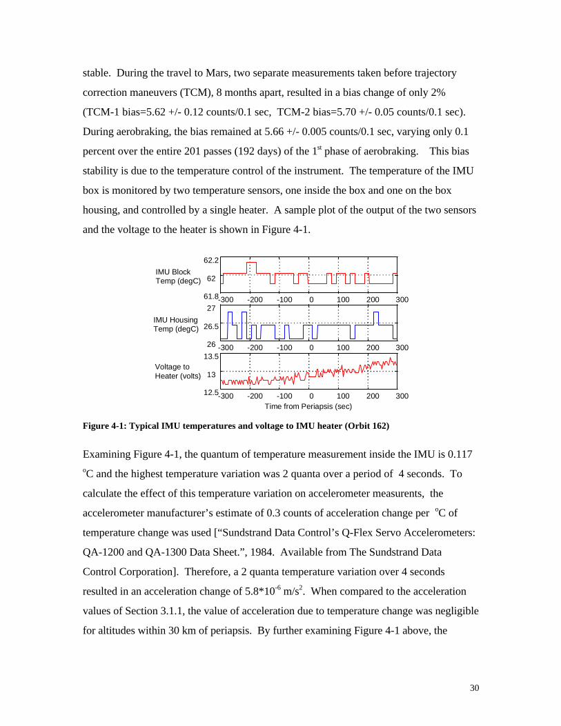
stability is due to the temperature control of the instrument. The temperature of the IMU

box is monitored by two temperature sensors, one inside the box and one on the box

housing, and controlled by a single heater. A sample plot of the output of the two sensors

and the voltage to the heater is shown in Figure 4-1.

-300 -200 -100 0 100 200 30061.8

62

62.2

IMU BlockTemp (degC)

-300 -200 -100 0 100 200 30026

26.5

27

IMU HousingTemp (degC)

-300 -200 -100 0 100 200 30012.5

13

13.5

Time from Periapsis (sec)

Voltage toHeater (volts)

Figure 4-1: Typical IMU temperatures and voltage to IMU heater (Orbit 162)

Examining Figure 4-1, the quantum of temperature measurement inside the IMU is 0.117oC and the highest temperature variation was 2 quanta over a period of 4 seconds. To

calculate the effect of this temperature variation on accelerometer measurents, the

accelerometer manufacturer’s estimate of 0.3 counts of acceleration change per oC of

temperature change was used [“Sundstrand Data Control’s Q-Flex Servo Accelerometers:

QA-1200 and QA-1300 Data Sheet.”, 1984. Available from The Sundstrand Data

Control Corporation]. Therefore, a 2 quanta temperature variation over 4 seconds

resulted in an acceleration change of 5.8*10-6 m/s2. When compared to the acceleration

values of Section 3.1.1, the value of acceleration due to temperature change was negligible

for altitudes within 30 km of periapsis. By further examining Figure 4-1 above, the

31

temperature did not exhibit any increase or decrease that would indicate atmospheric

heating was affecting the accelerometers inside the IMU.

4.3 Quantity of Accelerometer Data Necessary to PerformOperations

To determine the quantity of accelerometer data necessary to complete all

operational responsibilities, a simulation was developed to test the amount of

accelerometer data needed to reproduce a known atmospheric trend. The simulation

examined several different amounts of accelerometer data by first creating a atmosphere

with a known density trend, and then simulating the spacecraft with an accelerometer

instrument moving though that atmosphere. If the quantity of data being examined was

sufficient, the results from the model should reproduce the known atmosphere.

To set up the simulation the following parameters and assumptions were used. To

model the spacecraft motion, a 24 hour orbit (a=20180.3 e=0.827, i=93.175 deg,

w=320.037 deg, Ω=143.817 deg) was used. To model the accelerometer instrument,

Equation 3-1 was solved for the acceleration, aZ, and then this acceleration was quantized

and accumulated as described in Section 4.2. The coefficient of drag, spacecraft mass and

spacecraft cross-sectional area were all assumed to be constant (CD=2, mass=760 kg,

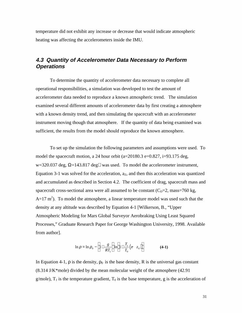
A=17 m2). To model the atmosphere, a linear temperature model was used such that the

density at any altitude was described by Equation 4-1 [Wilkerson, B., “Upper

Atmospheric Modeling for Mars Global Surveyor Aerobraking Using Least Squared

Processes,” Graduate Research Paper for George Washington University, 1998. Available

from author].

( )ln ln lnρ ρ= − +

+ −

0

1

1

001 1

g

RT

T

Tz z (4-1)

In Equation 4-1, ρ is the density, ρ0 is the base density, R is the universal gas constant

(8.314 J/K*mole) divided by the mean molecular weight of the atmosphere (42.91

g/mole), T1 is the temperature gradient, T0 is the base temperature, g is the acceleration of

32

gravity on Mars (3.4755 m/s2), z is the altitude, and z0 is the base altitude. For this

simulation, the following values were assumed: ρ0=60 kg/km3 , T1 = 2.862 K/km,

T0=131.2 K, zo=103 km.

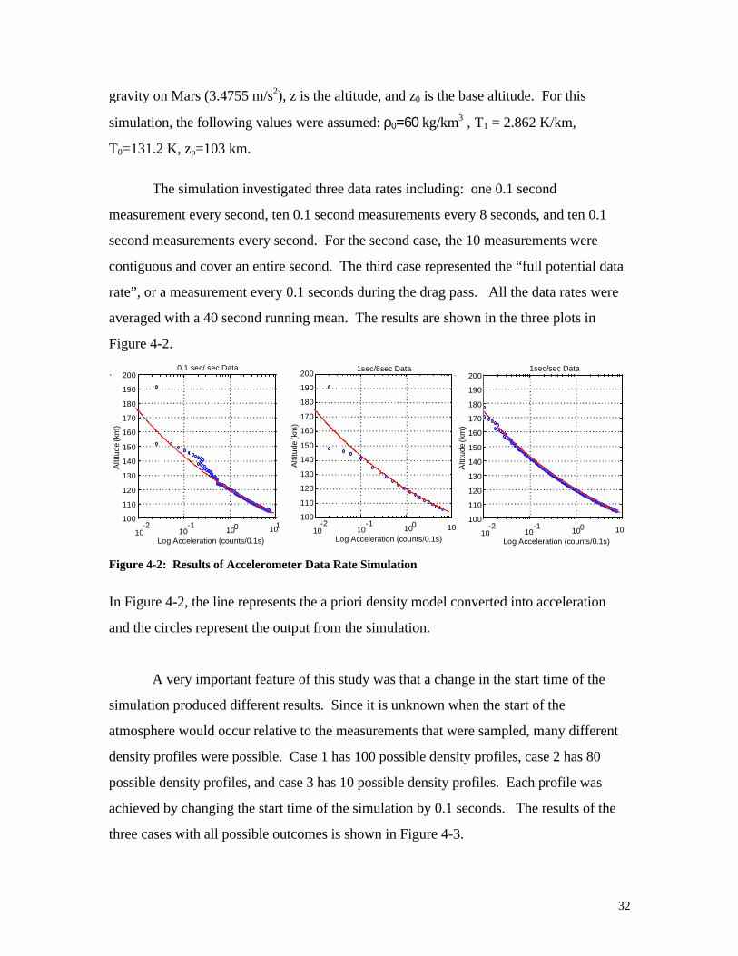
The simulation investigated three data rates including: one 0.1 second

measurement every second, ten 0.1 second measurements every 8 seconds, and ten 0.1

second measurements every second. For the second case, the 10 measurements were

contiguous and cover an entire second. The third case represented the “full potential data

rate”, or a measurement every 0.1 seconds during the drag pass. All the data rates were

averaged with a 40 second running mean. The results are shown in the three plots in

Figure 4-2.

10-2

10-1

100 101

Alti

tude

(km

)

Log Acceleration (counts/0.1s)

0.1 sec/ sec Data

100

110

120

130

140

150

160

170

180

190

2001sec/8sec Data 1sec/sec Data

10-2

10-1

100 10

Alti

tude

(km

)

Log Acceleration (counts/0.1s)

100

110

120

130

140

150

160

170

180

190

200

10-2

10-1

100 10

Alti

tude

(km

)

Log Acceleration (counts/0.1s)

100

110

120

130

140

150

160

170

180

190

200

Figure 4-2: Results of Accelerometer Data Rate Simulation

In Figure 4-2, the line represents the a priori density model converted into acceleration

and the circles represent the output from the simulation.

A very important feature of this study was that a change in the start time of the

simulation produced different results. Since it is unknown when the start of the

atmosphere would occur relative to the measurements that were sampled, many different

density profiles were possible. Case 1 has 100 possible density profiles, case 2 has 80

possible density profiles, and case 3 has 10 possible density profiles. Each profile was

achieved by changing the start time of the simulation by 0.1 seconds. The results of the

three cases with all possible outcomes is shown in Figure 4-3.

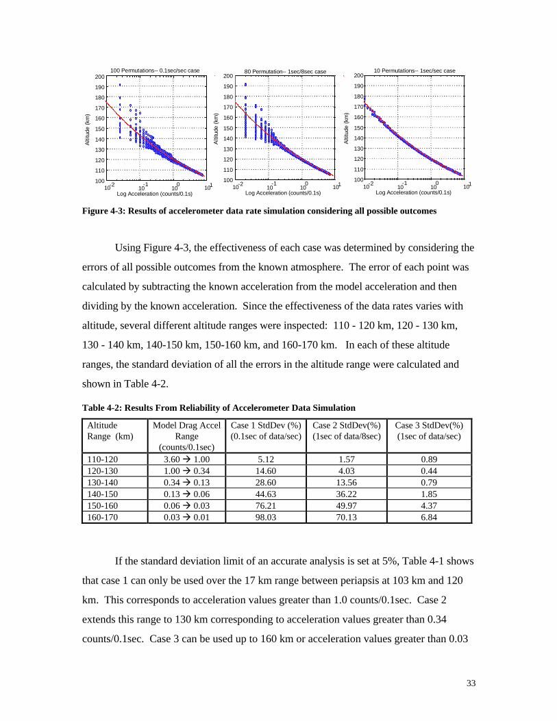
33

100 Permutations-- 0.1sec/sec case 80 Permutation-- 1sec/8sec case

Alti

tude

(km

)

10-2 10-1

100

101

Log Acceleration (counts/0.1s)

100

110

120

130

140

150

160

170

180

190

200

Alti

tude

(km

)

10-210

-110

0101

Log Acceleration (counts/0.1s)

100

110

120

130

140

150

160

170

180

190

20010 Permutations-- 1sec/sec case

Alti

tude

(km

)

10-2 10-1

100

101

Log Acceleration (counts/0.1s)

100

110

120

130

140

150

160

170

180

190

200

Figure 4-3: Results of accelerometer data rate simulation considering all possible outcomes

Using Figure 4-3, the effectiveness of each case was determined by considering the

errors of all possible outcomes from the known atmosphere. The error of each point was

calculated by subtracting the known acceleration from the model acceleration and then

dividing by the known acceleration. Since the effectiveness of the data rates varies with

altitude, several different altitude ranges were inspected: 110 - 120 km, 120 - 130 km,

130 - 140 km, 140-150 km, 150-160 km, and 160-170 km. In each of these altitude

ranges, the standard deviation of all the errors in the altitude range were calculated and

shown in Table 4-2.

Table 4-2: Results From Reliability of Accelerometer Data Simulation

AltitudeRange (km)

Model Drag AccelRange

(counts/0.1sec)

Case 1 StdDev (%)(0.1sec of data/sec)

Case 2 StdDev(%)(1sec of data/8sec)

Case 3 StdDev(%)(1sec of data/sec)

110-120 3.60 Æ 1.00 5.12 1.57 0.89120-130 1.00 Æ 0.34 14.60 4.03 0.44130-140 0.34 Æ 0.13 28.60 13.56 0.79140-150 0.13 Æ 0.06 44.63 36.22 1.85150-160 0.06 Æ 0.03 76.21 49.97 4.37160-170 0.03 Æ 0.01 98.03 70.13 6.84

If the standard deviation limit of an accurate analysis is set at 5%, Table 4-1 shows

that case 1 can only be used over the 17 km range between periapsis at 103 km and 120

km. This corresponds to acceleration values greater than 1.0 counts/0.1sec. Case 2

extends this range to 130 km corresponding to acceleration values greater than 0.34

counts/0.1sec. Case 3 can be used up to 160 km or acceleration values greater than 0.03

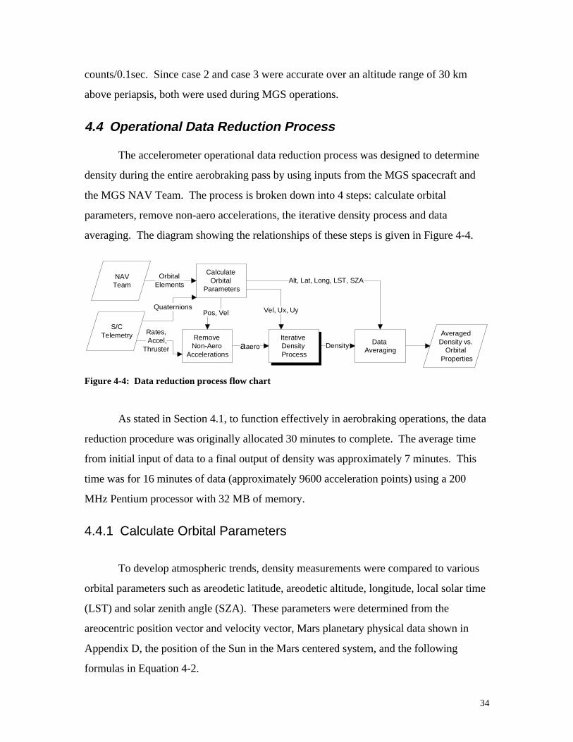
34

counts/0.1sec. Since case 2 and case 3 were accurate over an altitude range of 30 km

above periapsis, both were used during MGS operations.

4.4 Operational Data Reduction Process

The accelerometer operational data reduction process was designed to determine

density during the entire aerobraking pass by using inputs from the MGS spacecraft and

the MGS NAV Team. The process is broken down into 4 steps: calculate orbital

parameters, remove non-aero accelerations, the iterative density process and data

averaging. The diagram showing the relationships of these steps is given in Figure 4-4.

Calculate Orbital

Parameters

Remove Non-Aero

Accelerations

Iterative Density Process

Data Averaging

NAV Team

Averaged Density vs.

Orbital Properties

S/C Telemetry

Alt, Lat, Long, LST, SZA

Vel, Ux, UyPos, Vel

Orbital Elements

Quaternions

Rates, Accel,

Thruster aaero Density

Figure 4-4: Data reduction process flow chart

As stated in Section 4.1, to function effectively in aerobraking operations, the data

reduction procedure was originally allocated 30 minutes to complete. The average time

from initial input of data to a final output of density was approximately 7 minutes. This

time was for 16 minutes of data (approximately 9600 acceleration points) using a 200

MHz Pentium processor with 32 MB of memory.

4.4.1 Calculate Orbital Parameters

To develop atmospheric trends, density measurements were compared to various

orbital parameters such as areodetic latitude, areodetic altitude, longitude, local solar time

(LST) and solar zenith angle (SZA). These parameters were determined from the

areocentric position vector and velocity vector, Mars planetary physical data shown in

Appendix D, the position of the Sun in the Mars centered system, and the following

formulas in Equation 4-2.

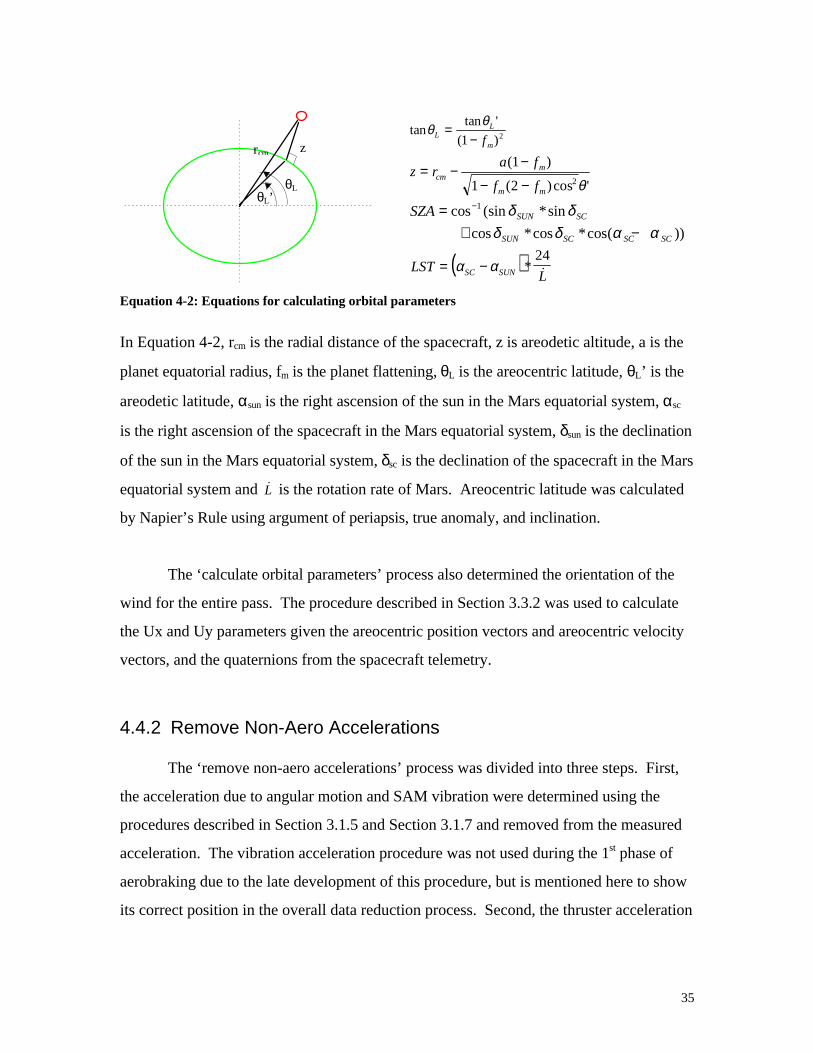
35

tantan '

( )θ

θL

L

mf=

−1 2

z ra f

f fcm

m

m m

= −−

− −

( )

( )cos '

1

1 2 2θ

SZA SUN SC

SUN SC SC SC

=+ −

−cos (sin *sin

cos *cos *cos( ))

1 δ δδ δ α α

( )LSTLSC SUN= −α α *

24

Equation 4-2: Equations for calculating orbital parameters

In Equation 4-2, rcm is the radial distance of the spacecraft, z is areodetic altitude, a is the

planet equatorial radius, fm is the planet flattening, θL is the areocentric latitude, θL’ is the

areodetic latitude, αsun is the right ascension of the sun in the Mars equatorial system, αsc

is the right ascension of the spacecraft in the Mars equatorial system, δsun is the declination

of the sun in the Mars equatorial system, δsc is the declination of the spacecraft in the Mars

equatorial system and L is the rotation rate of Mars. Areocentric latitude was calculated

by Napier’s Rule using argument of periapsis, true anomaly, and inclination.

The ‘calculate orbital parameters’ process also determined the orientation of the

wind for the entire pass. The procedure described in Section 3.3.2 was used to calculate

the Ux and Uy parameters given the areocentric position vectors and areocentric velocity

vectors, and the quaternions from the spacecraft telemetry.

4.4.2 Remove Non-Aero Accelerations

The ‘remove non-aero accelerations’ process was divided into three steps. First,

the acceleration due to angular motion and SAM vibration were determined using the

procedures described in Section 3.1.5 and Section 3.1.7 and removed from the measured

acceleration. The vibration acceleration procedure was not used during the 1st phase of

aerobraking due to the late development of this procedure, but is mentioned here to show

its correct position in the overall data reduction process. Second, the thruster acceleration

θL’θL

zrcm

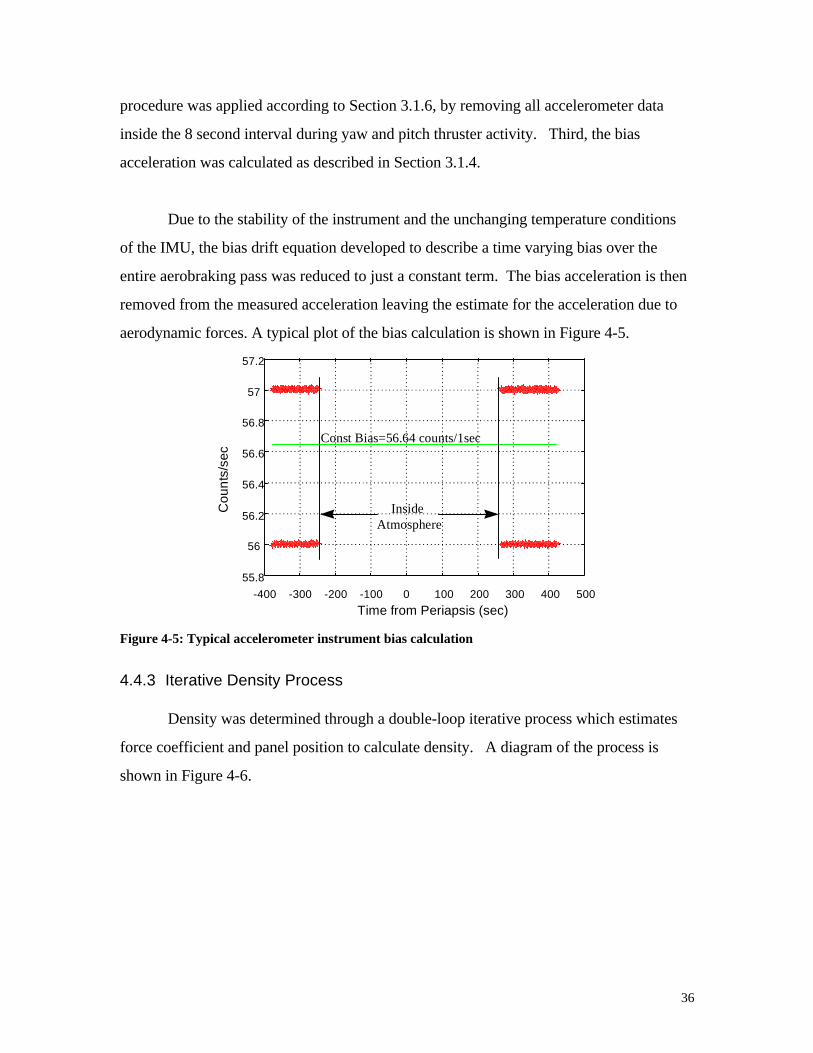
36

procedure was applied according to Section 3.1.6, by removing all accelerometer data

inside the 8 second interval during yaw and pitch thruster activity. Third, the bias

acceleration was calculated as described in Section 3.1.4.

Due to the stability of the instrument and the unchanging temperature conditions

of the IMU, the bias drift equation developed to describe a time varying bias over the

entire aerobraking pass was reduced to just a constant term. The bias acceleration is then

removed from the measured acceleration leaving the estimate for the acceleration due to

aerodynamic forces. A typical plot of the bias calculation is shown in Figure 4-5.

55.8

56

56.2

56.4

56.6

56.8

57

57.2

-400 -300 -200 -100 0 100 200 300 400 500

Time from Periapsis (sec)

Cou

nts

/sec

Inside Atmosphere

Const Bias=56.64 counts/1sec

Figure 4-5: Typical accelerometer instrument bias calculation

4.4.3 Iterative Density Process

Density was determined through a double-loop iterative process which estimates

force coefficient and panel position to calculate density. A diagram of the process is

shown in Figure 4-6.

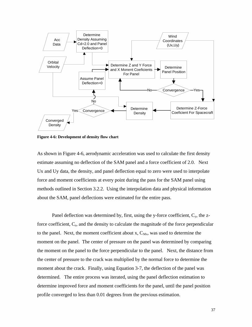
37

Acc Data

Determine Density Assuming Cd=2.0 and Panel

Deflection=0

Determine Z and Y Force and X Monent Coeficients

For Panel Assume Panel Deflection=0

Determine Panel Position

Determine Z-Force Coeficient For Spacecraft

Convergence

Determine Density

Convergence

Converged Density

No

Yes

No

Wind Coordinates

(Ux,Uy)

Yes

Orbital Velocity

Figure 4-6: Development of density flow chart

As shown in Figure 4-6, aerodynamic acceleration was used to calculate the first density

estimate assuming no deflection of the SAM panel and a force coefficient of 2.0. Next

Ux and Uy data, the density, and panel deflection equal to zero were used to interpolate

force and moment coefficients at every point during the pass for the SAM panel using

methods outlined in Section 3.2.2. Using the interpolation data and physical information

about the SAM, panel deflections were estimated for the entire pass.

Panel deflection was determined by, first, using the y-force coefficient, Cy, the z-

force coefficient, Cz, and the density to calculate the magnitude of the force perpendicular

to the panel. Next, the moment coefficient about x, CMx, was used to determine the

moment on the panel. The center of pressure on the panel was determined by comparing

the moment on the panel to the force perpendicular to the panel. Next, the distance from

the center of pressure to the crack was multiplied by the normal force to determine the

moment about the crack. Finally, using Equation 3-7, the deflection of the panel was

determined. The entire process was iterated, using the panel deflection estimation to

determine improved force and moment coefficients for the panel, until the panel position

profile converged to less than 0.01 degrees from the previous estimation.

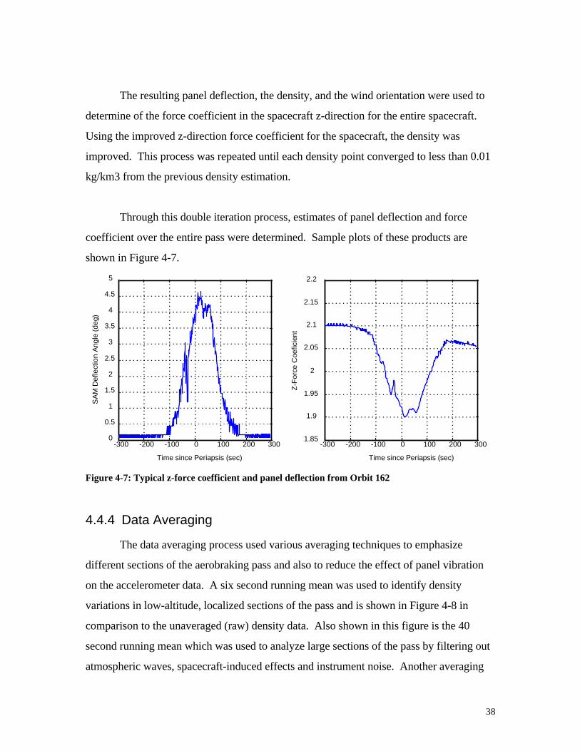
38

The resulting panel deflection, the density, and the wind orientation were used to

determine of the force coefficient in the spacecraft z-direction for the entire spacecraft.

Using the improved z-direction force coefficient for the spacecraft, the density was

improved. This process was repeated until each density point converged to less than 0.01

kg/km3 from the previous density estimation.

Through this double iteration process, estimates of panel deflection and force

coefficient over the entire pass were determined. Sample plots of these products are

shown in Figure 4-7.

-300 -200 -100 0 100 200 3001.85

1.9

1.95

2

2.05

2.1

2.15

2.2

Time since Periapsis (sec)

Z-F

orce

Coe

ficie

nt

-300 -200 -100 0 100 200 3000

0.5

1

1.5

2

2.5

3

3.5

4

4.5

5

SA

M D

efle

ctio

n A

ngle

(de

g)

Time since Periapsis (sec)

Figure 4-7: Typical z-force coefficient and panel deflection from Orbit 162

4.4.4 Data Averaging

The data averaging process used various averaging techniques to emphasize

different sections of the aerobraking pass and also to reduce the effect of panel vibration

on the accelerometer data. A six second running mean was used to identify density

variations in low-altitude, localized sections of the pass and is shown in Figure 4-8 in

comparison to the unaveraged (raw) density data. Also shown in this figure is the 40

second running mean which was used to analyze large sections of the pass by filtering out

atmospheric waves, spacecraft-induced effects and instrument noise. Another averaging

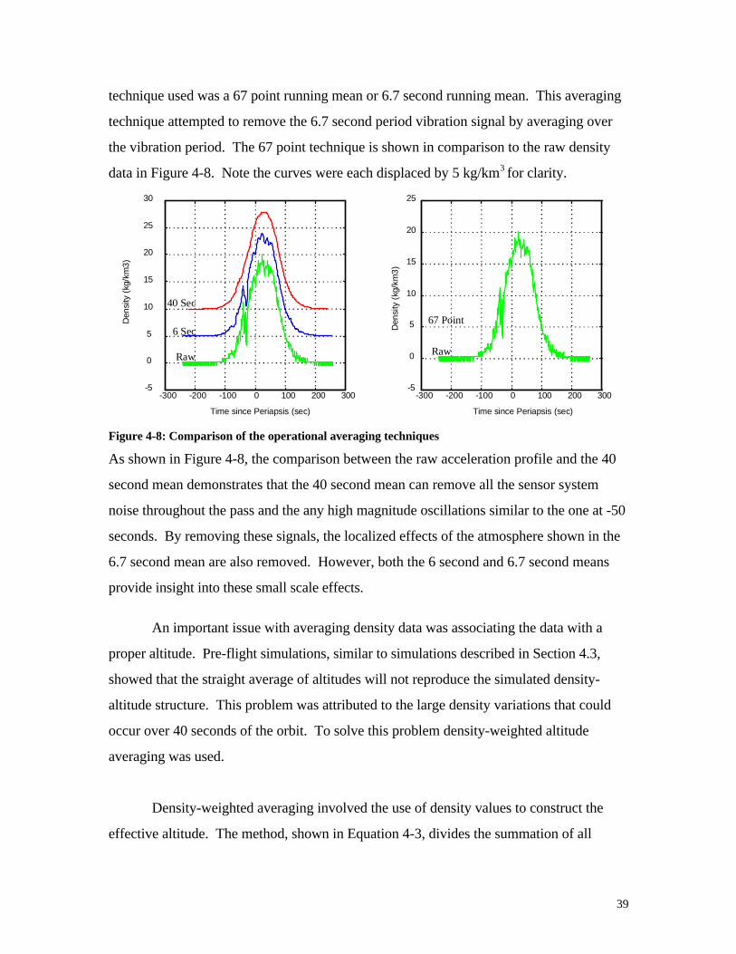
39

technique used was a 67 point running mean or 6.7 second running mean. This averaging

technique attempted to remove the 6.7 second period vibration signal by averaging over

the vibration period. The 67 point technique is shown in comparison to the raw density

data in Figure 4-8. Note the curves were each displaced by 5 kg/km3 for clarity.

-300 -200 -100 0 100 200 300-5

0

5

10

15

20

25

30

Time since Periapsis (sec)

-300 -200 -100 0 100 200 300-5

0

5

10

15

20

25

Time since Periapsis (sec)

Den

sity

(kg

/km

3)

Den

sity

(kg

/km

3)

6 Sec

40 Sec

Raw Raw

67 Point

Figure 4-8: Comparison of the operational averaging techniques

As shown in Figure 4-8, the comparison between the raw acceleration profile and the 40

second mean demonstrates that the 40 second mean can remove all the sensor system

noise throughout the pass and the any high magnitude oscillations similar to the one at -50

seconds. By removing these signals, the localized effects of the atmosphere shown in the

6.7 second mean are also removed. However, both the 6 second and 6.7 second means

provide insight into these small scale effects.

An important issue with averaging density data was associating the data with a

proper altitude. Pre-flight simulations, similar to simulations described in Section 4.3,

showed that the straight average of altitudes will not reproduce the simulated density-

altitude structure. This problem was attributed to the large density variations that could

occur over 40 seconds of the orbit. To solve this problem density-weighted altitude

averaging was used.

Density-weighted averaging involved the use of density values to construct the

effective altitude. The method, shown in Equation 4-3, divides the summation of all

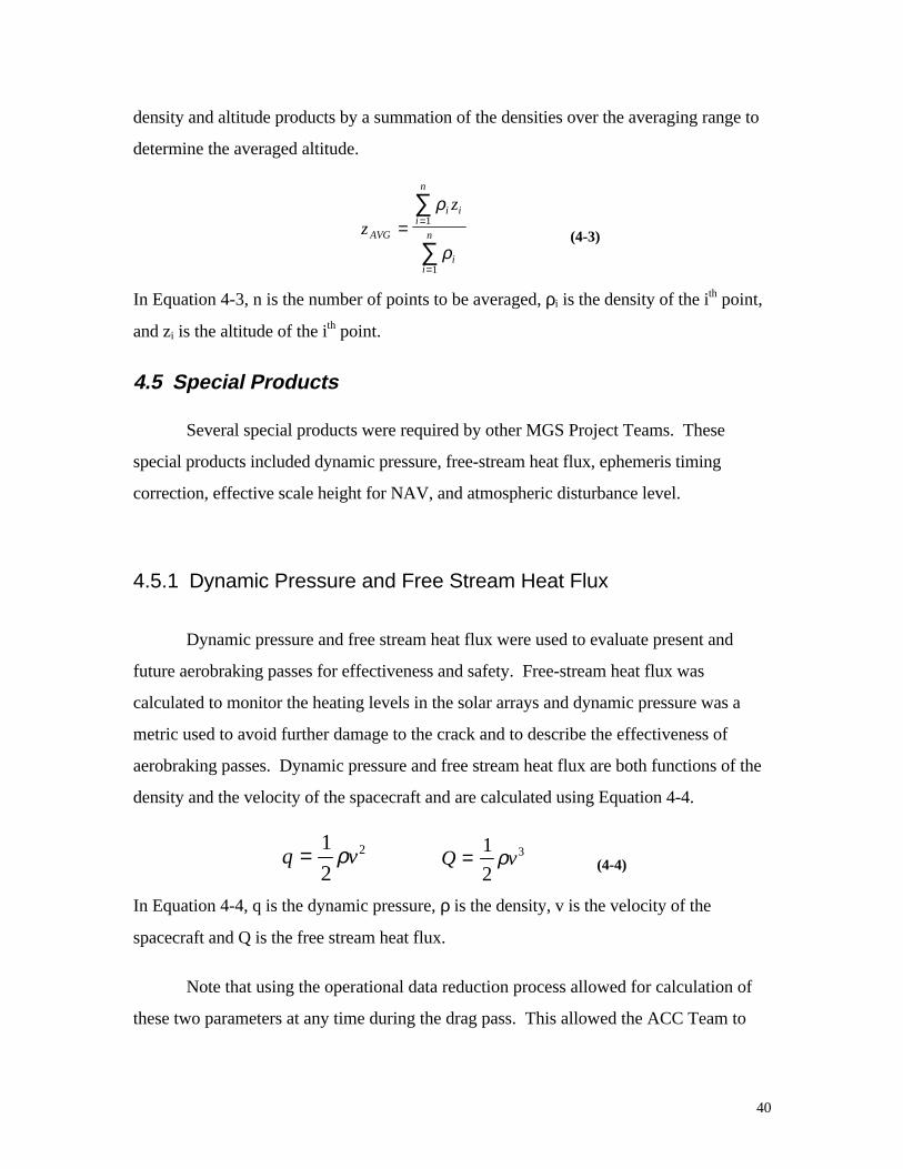
40

density and altitude products by a summation of the densities over the averaging range to

determine the averaged altitude.

z

z

AVG

i ii

n

ii

n= =

=

∑

∑

ρ

ρ

1

1

(4-3)

In Equation 4-3, n is the number of points to be averaged, ρi is the density of the ith point,

and zi is the altitude of the ith point.

4.5 Special Products

Several special products were required by other MGS Project Teams. These

special products included dynamic pressure, free-stream heat flux, ephemeris timing

correction, effective scale height for NAV, and atmospheric disturbance level.

4.5.1 Dynamic Pressure and Free Stream Heat Flux

Dynamic pressure and free stream heat flux were used to evaluate present and

future aerobraking passes for effectiveness and safety. Free-stream heat flux was

calculated to monitor the heating levels in the solar arrays and dynamic pressure was a

metric used to avoid further damage to the crack and to describe the effectiveness of

aerobraking passes. Dynamic pressure and free stream heat flux are both functions of the

density and the velocity of the spacecraft and are calculated using Equation 4-4.

q v= 1

22ρ Q v= 1

23ρ (4-4)

In Equation 4-4, q is the dynamic pressure, ρ is the density, v is the velocity of the

spacecraft and Q is the free stream heat flux.

Note that using the operational data reduction process allowed for calculation of

these two parameters at any time during the drag pass. This allowed the ACC Team to

41

calculate the maximum heat flux and dynamic pressure during each pass and also calculate

the time of these maximum points in relation to the periapsis of the orbit

4.5.2 Ephemeris Timing Correction

Since the NAV Team would only commit to periapsis timing errors less than 225

seconds [Personal Communication, P. Esposito, 6/96], a method for refining the peripasis

time to within 10 seconds was created. The product, called ephemeris timing correction

(ETC), was the time in seconds from the NAV estimated periapsis time to the time of

actual periapsis assuming a symmetrical atmosphere. A symmetrical atmosphere has no

latitudinal or longitudinal variation, i.e. densities encountered before periapsis are equal to

densities calculated after periapsis. To determine the ETC, the time corresponding to the

accelerometer measurements was shifted until all variation between pre- and post-periapsis

densities were minimized. The amount of time shift which minimizes this variation was the

ETC.

When tested on models with symmetric atmospheres, the ETC process could

detect errors in periapsis time on the order of 1 second. This process was not used during

aerobraking because NAV team timing errors were consistently less than 3 seconds and

average timing errors calculated with ETC were 10 seconds. This lack of accuracy in the

ETC product shows the very non-symmetric nature of the Martian atmosphere.

4.5.3 Effective Scale Height for NAV

As part of the orbit determination process, the NAV team estimated the density at

periapsis using a constant density scale height model of the atmosphere. Since the NAV

team could not determine scale height, a process was generated to use accelerometer data

to estimate a scale height that best describes the entire pass. This scale height was known

as ‘Effective Scale Height for NAV’.

The following procedure was used to calculate ‘Effective Scale Height for NAV’.

First, the density calculated at periapsis by the accelerometer was assumed to be the

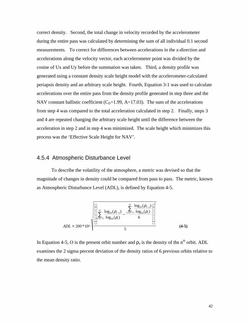
42

correct density. Second, the total change in velocity recorded by the accelerometer

during the entire pass was calculated by determining the sum of all individual 0.1 second

measurements. To correct for differences between accelerations in the z-direction and

accelerations along the velocity vector, each accelerometer point was divided by the

cosine of Ux and Uy before the summation was taken. Third, a density profile was

generated using a constant density scale height model with the accelerometer-calculated

periapsis density and an arbitrary scale height. Fourth, Equation 3-1 was used to calculate

accelerations over the entire pass from the density profile generated in step three and the

NAV constant ballistic coefficient (CD=1.99, A=17.03). The sum of the accelerations

from step 4 was compared to the total acceleration calculated in step 2. Finally, steps 3

and 4 are repeated changing the arbitrary scale height until the difference between the

acceleration in step 2 and in step 4 was minimized. The scale height which minimizes this

process was the ‘Effective Scale Height for NAV’.

4.5.4 Atmospheric Disturbance Level

To describe the volatility of the atmosphere, a metric was devised so that the

magnitude of changes in density could be compared from pass to pass. The metric, known

as Atmospheric Disturbance Level (ADL), is defined by Equation 4-5.

ADL

i

ii O

Oi

ii O

O

=

−

−

= −

−

= −∑∑

200 10

6

5

10 1

105

10 1

105

2

* ^

log ( )

log ( )

log ( )

log ( )ρρ

ρρ

(4-5)

In Equation 4-5, O is the present orbit number and ρn is the density of the nth orbit. ADL

examines the 2 sigma percent deviation of the density ratios of 6 previous orbits relative to

the mean density ratio.

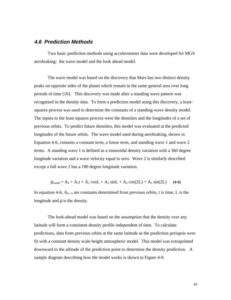
43

4.6 Prediction Methods

Two basic prediction methods using accelerometer data were developed for MGS

aerobraking: the wave model and the look ahead model.

The wave model was based on the discovery that Mars has two distinct density

peaks on opposite sides of the planet which remain in the same general area over long

periods of time [16]. This discovery was made after a standing wave pattern was

recognized in the density data. To form a prediction model using this discovery, a least-

squares process was used to determine the constants of a standing-wave density model.

The inputs to the least squares process were the densities and the longitudes of a set of

previous orbits. To predict future densities, this model was evaluated at the predicted

longitudes of the future orbits. The wave model used during aerobraking, shown in

Equation 4-6, contains a constant term, a linear term, and standing wave 1 and wave 2

terms. A standing wave 1 is defined as a sinusoidal density variation with a 360 degree

longitude variation and a wave velocity equal to zero. Wave 2 is similarly described

except a full wave 2 has a 180 degree longitude variation.

ρmodel = A0 + A1t + A2 cosL + A3 sinL + A4 cos(2L) + A5 sin(2L) (4-6)

In equation 4-6, A0->5 are constants determined from previous orbits, t is time, L is the

longitude and ρ is the density.

The look-ahead model was based on the assumption that the density over any

latitude will form a consistent density profile independent of time. To calculate

predictions, data from previous orbits at the same latitude as the prediction periapsis were

fit with a constant density scale height atmospheric model. This model was extrapolated

downward to the altitude of the prediction point to determine the density prediction. A

sample diagram describing how the model works is shown in Figure 4-9.

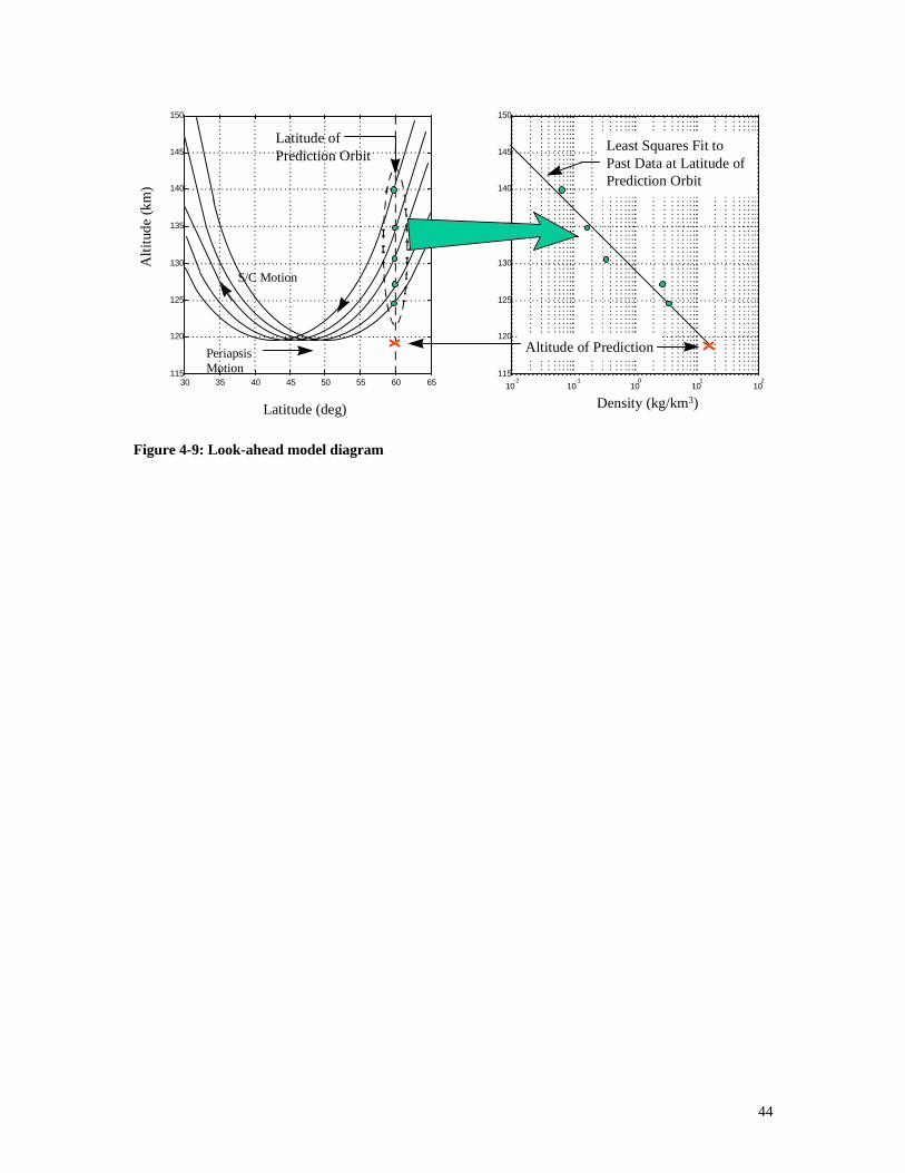
44

30 35 40 45 50 55 60 65115

120

125

130

135

140

145

150

10-2

10-1

100

101

102

115

120

125

130

135

140

145

150

Latitude (deg)

Alti

tud

e (k

m)

Density (kg/km3)

S/C Motion

Periapsis Motion

Latitude of Prediction Orbit

Altitude of Prediction

Least Squares Fit to Past Data at Latitude of Prediction Orbit

Figure 4-9: Look-ahead model diagram

45

5. Analysis of Process Errors

Section 5 analyzes the error induced into the calculations of density by the

operational methods described in Section 4. The total induced error can be determined by

the root-mean square of all the possible errors inherent to these methods. These error

sources include:

1. Ephemeris errors2. Errors in determining ballistic coefficient3. Errors in determining bias4. Digitization errors due to the accelerometer instrument

5.1 Ephemeris Errors

Ephemeris errors include errors from the use of periapsis osculating elements away

from periapsis, and timing and altitude errors from orbital elements generated by the NAV

Team. Errors from the use of osculating elements are described in Section 3.2. Timing

error is the amount of time that elapses from the actual periapsis point to the one predicted

by the NAV Team, assuming the orbit is correct. Altitude error is the error in altitude

assuming the timing of periapsis is correct. From discussions with the NAV Team

[Personal Communication, P. Esposito, 6/96], the ephemeris errors in a reconstructed

orbit were estimated at 0.1 km in altitude and 0.1 second in time.

Total altitude error is the combination of the range errors in Section 3.2 and NAV

altitude errors. The equivalent density error was determined by solving the equation of a

standard exponential atmosphere (ρ= ρΟ exp[∆H/HS] ) for density ratio, ρ/ρο, assuming a

scale height, HS, of 7 km and a ∆H of the corresponding total altitude error. The results

of the total altitude error for several altitude ranges are shown in Table 5-1.

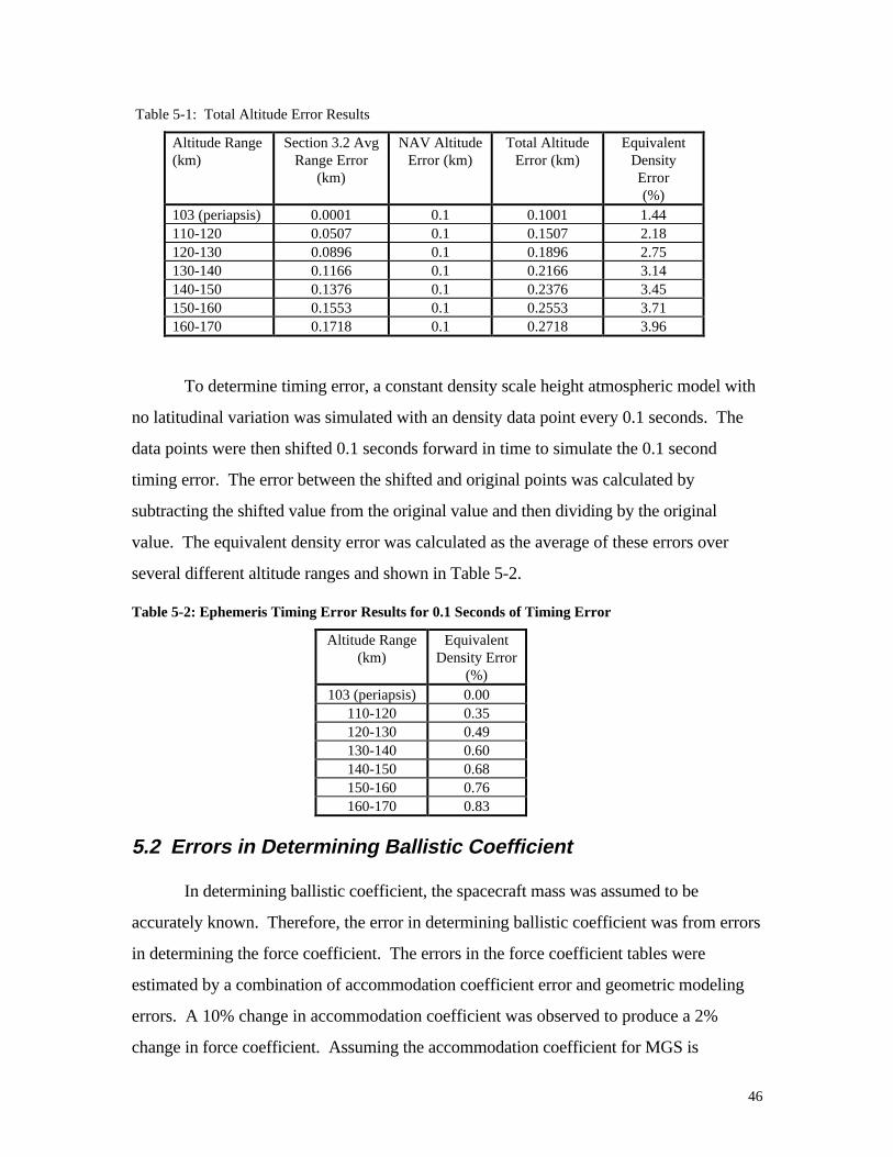
46

Table 5-1: Total Altitude Error Results

Altitude Range(km)

Section 3.2 AvgRange Error

(km)

NAV AltitudeError (km)

Total AltitudeError (km)

EquivalentDensityError(%)

103 (periapsis) 0.0001 0.1 0.1001 1.44110-120 0.0507 0.1 0.1507 2.18120-130 0.0896 0.1 0.1896 2.75130-140 0.1166 0.1 0.2166 3.14140-150 0.1376 0.1 0.2376 3.45150-160 0.1553 0.1 0.2553 3.71160-170 0.1718 0.1 0.2718 3.96

To determine timing error, a constant density scale height atmospheric model with

no latitudinal variation was simulated with an density data point every 0.1 seconds. The

data points were then shifted 0.1 seconds forward in time to simulate the 0.1 second

timing error. The error between the shifted and original points was calculated by

subtracting the shifted value from the original value and then dividing by the original

value. The equivalent density error was calculated as the average of these errors over

several different altitude ranges and shown in Table 5-2.

Table 5-2: Ephemeris Timing Error Results for 0.1 Seconds of Timing Error

Altitude Range(km)

EquivalentDensity Error

(%)103 (periapsis) 0.00

110-120 0.35120-130 0.49130-140 0.60140-150 0.68150-160 0.76160-170 0.83

5.2 Errors in Determining Ballistic Coefficient

In determining ballistic coefficient, the spacecraft mass was assumed to be

accurately known. Therefore, the error in determining ballistic coefficient was from errors

in determining the force coefficient. The errors in the force coefficient tables were

estimated by a combination of accommodation coefficient error and geometric modeling

errors. A 10% change in accommodation coefficient was observed to produce a 2%

change in force coefficient. Assuming the accommodation coefficient for MGS is

47

between 0.95 and 1.0 results in a 1% error in force coefficient. Error in force coefficient

due to geometric model imperfections was estimated at 2% [Personal Communication, R.

Wilmoth, 9/14/98]. Therefore, the error inherent to the calculation of force coefficient

tables is the root-mean square of the accomodation coefficient and model imperfections

errors or 2.24%. To determine total error in force coefficient, the inputs to the

interpolation of the force coefficient tables, wind orientation and panel deflection, were

also considered.

To calculate the wind orientation error, a 1 degree error in wind orientation was

assumed. The greatest variation in the interpolation tables shows Cz changes from 2.12

for the free molecular table with Ux=Uy=0 to 1.98 for the free molecular table with

Uy=10 degrees. This constitutes a 0.0134 Cz change per degree of orientation error which

can be used to state that a 1 degree orientation error will cause a 0.65 % error in density

estimation.

For determining error in calculation of panel deflection, the panel position

calculated using methods from Section 4.4.3 and the panel deflection calculated from sun

sensor data were compared. The greatest difference between the two independent

calculations inside the atmosphere is approximately 1 degree. Using a similar method to

the one used above, the greatest variation in the interpolation tables occurs from 2.12 for

the free molecular table, with no panel deflection to 2.0194 for the free molecular table

with 10 degrees panel deflection. This constitutes a 0.01006 Cz change per degree of panel

deflection error which was used to state that a 1 degree deflection error will cause a 0.47

% error in density estimation.

5.3 Errors in Determining Bias

The average standard error in determining the bias was 0.005 counts/0.1 seconds.

By simulating a sample pass using a linear temperature profile described in Section 4.2, the

counts every 0.1 second can be determined at various altitude levels. By assuming a

0.005 counts/0.1 second error on each acceleration value, an error can be identified as a

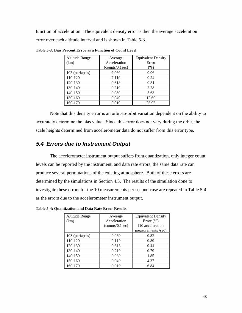
48

function of acceleration. The equivalent density error is then the average acceleration

error over each altitude interval and is shown in Table 5-3.

Table 5-3: Bias Percent Error as a Function of Count Level

Altitude Range(km)

AverageAcceleration

(counts/0.1sec)

Equivalent DensityError(%)

103 (periapsis) 9.060 0.06110-120 2.119 0.24120-130 0.618 0.81130-140 0.219 2.28140-150 0.089 5.63150-160 0.040 12.60160-170 0.019 25.95

Note that this density error is an orbit-to-orbit variation dependent on the ability to

accurately determine the bias value. Since this error does not vary during the orbit, the

scale heights determined from accelerometer data do not suffer from this error type.

5.4 Errors due to Instrument Output

The accelerometer instrument output suffers from quantization, only integer count

levels can be reported by the instrument, and data rate errors, the same data rate can

produce several permutations of the existing atmosphere. Both of these errors are

determined by the simulations in Section 4.3. The results of the simulation done to

investigate these errors for the 10 measurements per second case are repeated in Table 5-4

as the errors due to the accelerometer instrument output.

Table 5-4: Quantization and Data Rate Error Results

Altitude Range(km)

AverageAcceleration

(counts/0.1sec)

Equivalent DensityError (%)

(10 accelerationmeasurements /sec)

103 (periapsis) 9.060 0.82110-120 2.119 0.89120-130 0.618 0.44130-140 0.219 0.79140-150 0.089 1.85150-160 0.040 4.37160-170 0.019 6.84

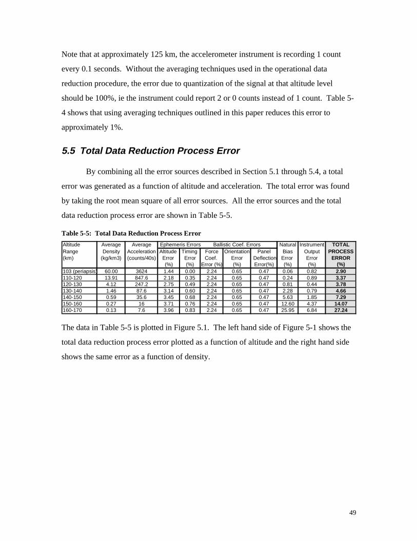
49

Note that at approximately 125 km, the accelerometer instrument is recording 1 count

every 0.1 seconds. Without the averaging techniques used in the operational data

reduction procedure, the error due to quantization of the signal at that altitude level

should be 100%, ie the instrument could report 2 or 0 counts instead of 1 count. Table 5-

4 shows that using averaging techniques outlined in this paper reduces this error to

approximately 1%.

5.5 Total Data Reduction Process Error

By combining all the error sources described in Section 5.1 through 5.4, a total

error was generated as a function of altitude and acceleration. The total error was found

by taking the root mean square of all error sources. All the error sources and the total

data reduction process error are shown in Table 5-5.

Table 5-5: Total Data Reduction Process Error

Altitude Average Average Ephemeris Errors Ballistic Coef. Errors Natural Instrument TOTALRange Density Acceleration Altitude Timing Force Orientation Panel Bias Output PROCESS(km) (kg/km3) (counts/40s) Error Error Coef. Error Deflection Error Error ERROR

(%) (%) Error (%) (%) Error(%) (%) (%) (%)103 (periapsis) 60.00 3624 1.44 0.00 2.24 0.65 0.47 0.06 0.82 2.90110-120 13.91 847.6 2.18 0.35 2.24 0.65 0.47 0.24 0.89 3.37120-130 4.12 247.2 2.75 0.49 2.24 0.65 0.47 0.81 0.44 3.78130-140 1.46 87.6 3.14 0.60 2.24 0.65 0.47 2.28 0.79 4.66140-150 0.59 35.6 3.45 0.68 2.24 0.65 0.47 5.63 1.85 7.29150-160 0.27 16 3.71 0.76 2.24 0.65 0.47 12.60 4.37 14.07160-170 0.13 7.6 3.96 0.83 2.24 0.65 0.47 25.95 6.84 27.24

The data in Table 5-5 is plotted in Figure 5.1. The left hand side of Figure 5-1 shows the

total data reduction process error plotted as a function of altitude and the right hand side

shows the same error as a function of density.

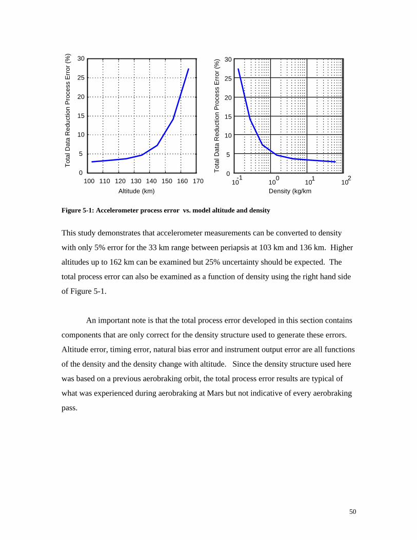
50

100 110 120 130 140 150 160 1700

5

10

15

20

25

30

Altitude (km)

Tot

al D

ata

Red

uct

ion

Pro

cess

Err

or (

%)

10-1

100

101

102

0

5

10

15

20

25

30

Density (kg/km

Tot

al D

ata

Red

uct

ion

Pro

cess

Err

or (

%)

Figure 5-1: Accelerometer process error vs. model altitude and density

This study demonstrates that accelerometer measurements can be converted to density

with only 5% error for the 33 km range between periapsis at 103 km and 136 km. Higher

altitudes up to 162 km can be examined but 25% uncertainty should be expected. The

total process error can also be examined as a function of density using the right hand side

of Figure 5-1.

An important note is that the total process error developed in this section contains

components that are only correct for the density structure used to generate these errors.

Altitude error, timing error, natural bias error and instrument output error are all functions

of the density and the density change with altitude. Since the density structure used here

was based on a previous aerobraking orbit, the total process error results are typical of

what was experienced during aerobraking at Mars but not indicative of every aerobraking

pass.

51

6. Verification of Accelerometer Results

Section 6 presents the studies done to verify the accelerometer data reduction

procedure outlined in Section 4. Studies were also performed to verify the effectiveness

of prediction schemes described in Section 4.6.

6.1 Data Reduction Process Verification

To verify the accelerometer data reduction process, two data products were

examined. The first product, SAM panel deflection, was estimated during the density

iteration scheme. The Spacecraft (S/C) Team also calculated panel deflection by using

spacecraft attitude data and data from sun sensors on the SAM. The second product,

change in orbital period, was estimated by the ACC Team and the NAV Team.

6.1.1 Panel Deflection Comparison: ACC vs. Sun Sensor

For all orbits in which SAM deflection angle was calculated using the sun sensor,

the accelerometer calculated panel deflection was always within 1.5 degrees of the sun

sensor data. Four passes are shown as examples of this accuracy. Passes 50, 100, 125

and 162 are shown in Figure 6-1.

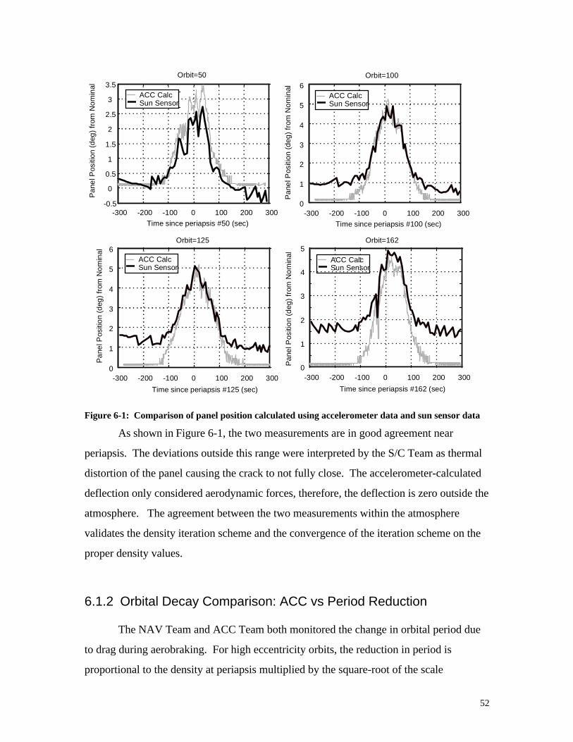
52

-300 -200 -100 0 100 200 300-0.5

0

0.5

1

1.5

2

2.5

3

3.5Orbit=50

Time since periapsis #50 (sec)

Pan

el P

ositi

on (

deg)

from

Nom

inal

ACC Calc Sun Sensor

-300 -200 -100 0 100 200 3000

1

2

3

4

5

6Orbit=100

Time since periapsis #100 (sec)

Pan

el P

ositi

on (

deg)

from

Nom

inal

ACC Calc Sun Sensor

-300 -200 -100 0 100 200 3000

1

2

3

4

5

6Orbit=125

Time since periapsis #125 (sec)

Pan

el P

ositi

on (

deg)

from

Nom

inal

ACC Calc Sun Sensor

ACC Calc Sun Sensor

-300 -200 -100 0 100 200 3000

1

2

3

4

5Orbit=162

Time since periapsis #162 (sec)

Pan

el P

ositi

on (

deg)

from

Nom

inal

Figure 6-1: Comparison of panel position calculated using accelerometer data and sun sensor data

As shown in Figure 6-1, the two measurements are in good agreement near

periapsis. The deviations outside this range were interpreted by the S/C Team as thermal

distortion of the panel causing the crack to not fully close. The accelerometer-calculated

deflection only considered aerodynamic forces, therefore, the deflection is zero outside the

atmosphere. The agreement between the two measurements within the atmosphere

validates the density iteration scheme and the convergence of the iteration scheme on the

proper density values.

6.1.2 Orbital Decay Comparison: ACC vs Period Reduction

The NAV Team and ACC Team both monitored the change in orbital period due

to drag during aerobraking. For high eccentricity orbits, the reduction in period is

proportional to the density at periapsis multiplied by the square-root of the scale

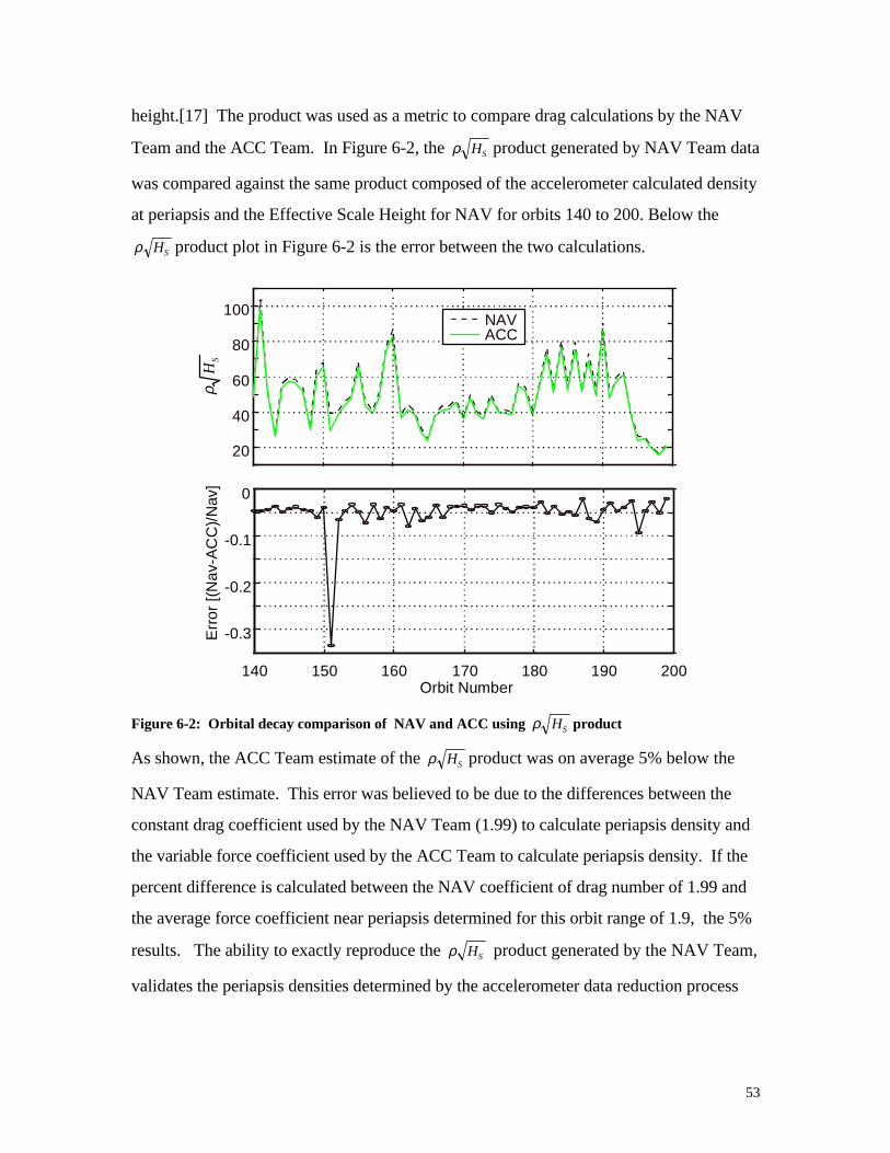
53

height.[17] The product was used as a metric to compare drag calculations by the NAV

Team and the ACC Team. In Figure 6-2, the ρ HS product generated by NAV Team data

was compared against the same product composed of the accelerometer calculated density

at periapsis and the Effective Scale Height for NAV for orbits 140 to 200. Below the

ρ HS product plot in Figure 6-2 is the error between the two calculations.

140 150 160 170 180 190 200

-0.3

-0.2

-0.1

0

Err

or [(

Nav

-AC

C)/

Nav

]

Orbit Number

20

40

60

80

100

ACCNAV

ρH

S

Figure 6-2: Orbital decay comparison of NAV and ACC using ρ HS product

As shown, the ACC Team estimate of the ρ HS product was on average 5% below the

NAV Team estimate. This error was believed to be due to the differences between the

constant drag coefficient used by the NAV Team (1.99) to calculate periapsis density and

the variable force coefficient used by the ACC Team to calculate periapsis density. If the

percent difference is calculated between the NAV coefficient of drag number of 1.99 and

the average force coefficient near periapsis determined for this orbit range of 1.9, the 5%

results. The ability to exactly reproduce the ρ HS product generated by the NAV Team,

validates the periapsis densities determined by the accelerometer data reduction process

54

and the method for isolating acceleration due to aerodynamic forces from the measured

acceleration over the entire pass.

The ‘Effective Scale Height for NAV’ product was also validated using the

ρ HS product. Two simulation runs of aerobraking passes were made, first with the NAV

Team scale height and then with the ACC Team effective scale heights. The results of

these tests are shown in Table 6-1 [Personal Communication, P.Esposito, 12/11/97].

Table 6-1: Results of NAV Simulation Runs with Accelerometer Calculated Effective Scale Height

PassNumber

NAV ScaleHeight

NAV DensityUsing NAV Hs

ACC EffectiveScale Height

NAV DensityUsing ACC Hs

ACCCalculated

Density59 7.0 8.83 11.5 6.92 7.2360 7.0 12.90 6.21 13.55 14.60

Comparing the NAV density calculated using the NAV scale height to the ACC density

values resulted in a 22% error for pass 59 and a 12% error for pass 60. If the NAV

density is re-calculated using the ACC effective scale height, the error between NAV

density and accelerometer density was reduced to 4% for pass 59 and 7% for pass 60.

This demonstrates not only the dependence of the NAV Team on proper scale height

information but how much improvement can be made on orbit determination when a more

precise calculation of scale height can be made.

6.2 Prediction Scheme Verification

To verify the prediction methods, densities of previous passes were predicted and

compared to the actual density calculated for that orbit. Prior to aerobraking the MGS

project estimated the variability inherent to the Martian atmosphere at a two sigma value

of 70%. Therefore, an accurate prediction method is one that could consistently predict

upcoming densities below this variability value.

Several prediction schemes were used during aerobraking. These schemes

included: Persistence, which used scale height and density of the previous pass to predict

one orbit ahead; 5-Orbit Mean, which used 5 previous densities, scaled to the

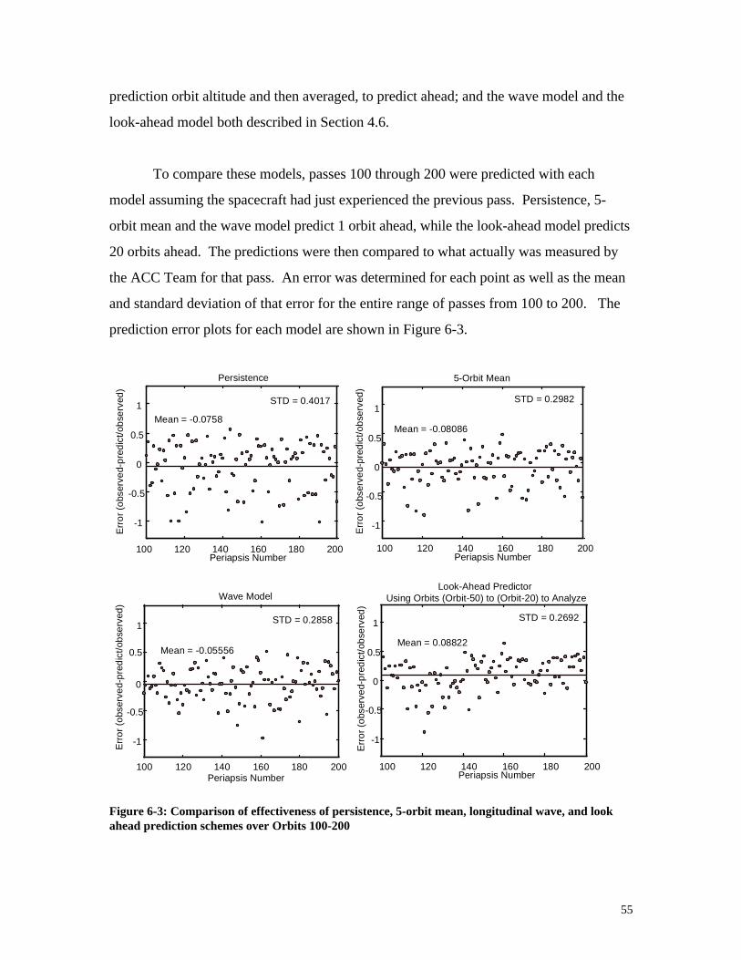
55

prediction orbit altitude and then averaged, to predict ahead; and the wave model and the

look-ahead model both described in Section 4.6.

To compare these models, passes 100 through 200 were predicted with each

model assuming the spacecraft had just experienced the previous pass. Persistence, 5-

orbit mean and the wave model predict 1 orbit ahead, while the look-ahead model predicts

20 orbits ahead. The predictions were then compared to what actually was measured by

the ACC Team for that pass. An error was determined for each point as well as the mean

and standard deviation of that error for the entire range of passes from 100 to 200. The

prediction error plots for each model are shown in Figure 6-3.

-1

-0.5

0

0.5

1

100 120 140 160 180 200Periapsis Number

Err

or (

obse

rved

-pre

dict

/obs

erve

d)

Persistence

Mean = -0.0758

STD = 0.4017

-1

-0.5

0

0.5

1

100 120 140 160 180 200Periapsis Number

Err

or (

obse

rved

-pre

dict

/obs

erve

d)

5-Orbit Mean

Mean = -0.08086

STD = 0.2982

100 120 140 160 180 200

-1

-0.5

0

0.5

1

Periapsis Number

Err

or (

obse

rved

-pre

dict

/obs

erve

d)

Wave Model

Mean = -0.05556

STD = 0.2858

Err

or (

obse

rved

-pre

dict

/obs

erve

d)

100 120 140 160 180 200

-1

-0.5

0

0.5

1

Periapsis Number

Look-Ahead Predictor Using Orbits (Orbit-50) to (Orbit-20) to Analyze

Mean = 0.08822

STD = 0.2692

Figure 6-3: Comparison of effectiveness of persistence, 5-orbit mean, longitudinal wave, and lookahead prediction schemes over Orbits 100-200

56

Each model predicted the mean within 9% of the actual, however, the standard

deviations of each model vary from 40% for the persistence model to 27% for the look-

ahead model. The wave model, used for predictions during aerobraking, has a standard

deviation of 29%, or a 2 sigma variability of 58%. This value was below the 2 sigma

atmospheric variability parameter of 70% and, therefore, the predictions made by the ACC

Team during the first phase of aerobraking were within the constraints originally set by the

MGS project.

An important note, by examining the persistence model, the actual atmospheric

variability of the atmosphere over this range of orbits can be determined. The two sigma

atmospheric variability is approximately 80%. This value is slightly higher than the pre-

aerobraking project estimate of 70%.

For predicting one orbit ahead the wave model produces the lowest standard

deviation of all the methods and also produces the most accurate results (wave model had

the lowest mean error of all prediction methods). The results from the look-ahead model

demonstrate that accurate long range predictions, up to 20 orbits into the future, are

possible. Therefore, a new direction for predictions with accelerometer data could be the

combination of the wave model and the look-ahead model into an accurate short range

and long range predictor.

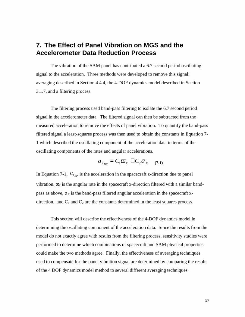
57

7. The Effect of Panel Vibration on MGS and theAccelerometer Data Reduction Process

The vibration of the SAM panel has contributed a 6.7 second period oscillating

signal to the acceleration. Three methods were developed to remove this signal:

averaging described in Section 4.4.4, the 4-DOF dynamics model described in Section

3.1.7, and a filtering process.

The filtering process used band-pass filtering to isolate the 6.7 second period

signal in the accelerometer data. The filtered signal can then be subtracted from the

measured acceleration to remove the effects of panel vibration. To quantify the band-pass

filtered signal a least-squares process was then used to obtain the constants in Equation 7-

1 which described the oscillating component of the acceleration data in terms of the

oscillating components of the rates and angular accelerations.

a C CZ X XBP= +1 2ω α (7-1)

In Equation 7-1, azBP is the acceleration in the spacecraft z-direction due to panel

vibration, ωX is the angular rate in the spacecraft x-direction filtered with a similar band-

pass as above, αX is the band-pass filtered angular acceleration in the spacecraft x-

direction, and C1 and C2 are the constants determined in the least squares process.

This section will describe the effectiveness of the 4-DOF dynamics model in

determining the oscillating component of the acceleration data. Since the results from the

model do not exactly agree with results from the filtering process, sensitivity studies were

performed to determine which combinations of spacecraft and SAM physical properties

could make the two methods agree. Finally, the effectiveness of averaging techniques

used to compensate for the panel vibration signal are determined by comparing the results

of the 4 DOF dynamics model method to several different averaging techniques.

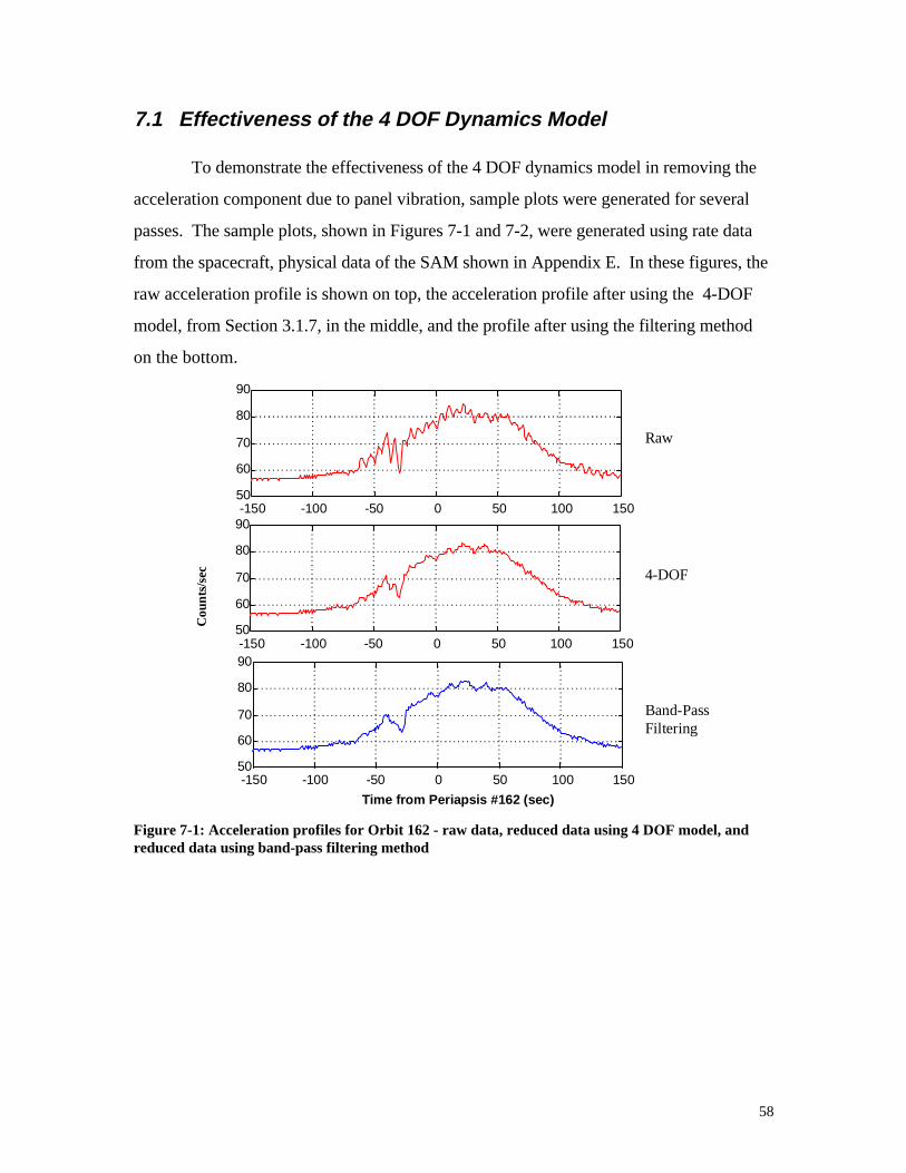
58

7.1 Effectiveness of the 4 DOF Dynamics Model

To demonstrate the effectiveness of the 4 DOF dynamics model in removing the

acceleration component due to panel vibration, sample plots were generated for several

passes. The sample plots, shown in Figures 7-1 and 7-2, were generated using rate data

from the spacecraft, physical data of the SAM shown in Appendix E. In these figures, the

raw acceleration profile is shown on top, the acceleration profile after using the 4-DOF

model, from Section 3.1.7, in the middle, and the profile after using the filtering method

on the bottom.

-150 -100 -50 0 50 100 15050

60

70

80

90

-150 -100 -50 0 50 100 15050

60

70

80

90-150 -100 -50 0 50 100 15050

60

70

80

90

Time from Periapsis #162 (sec)

Cou

nts/

sec

Raw

4-DOF

Band-PassFiltering

Figure 7-1: Acceleration profiles for Orbit 162 - raw data, reduced data using 4 DOF model, andreduced data using band-pass filtering method

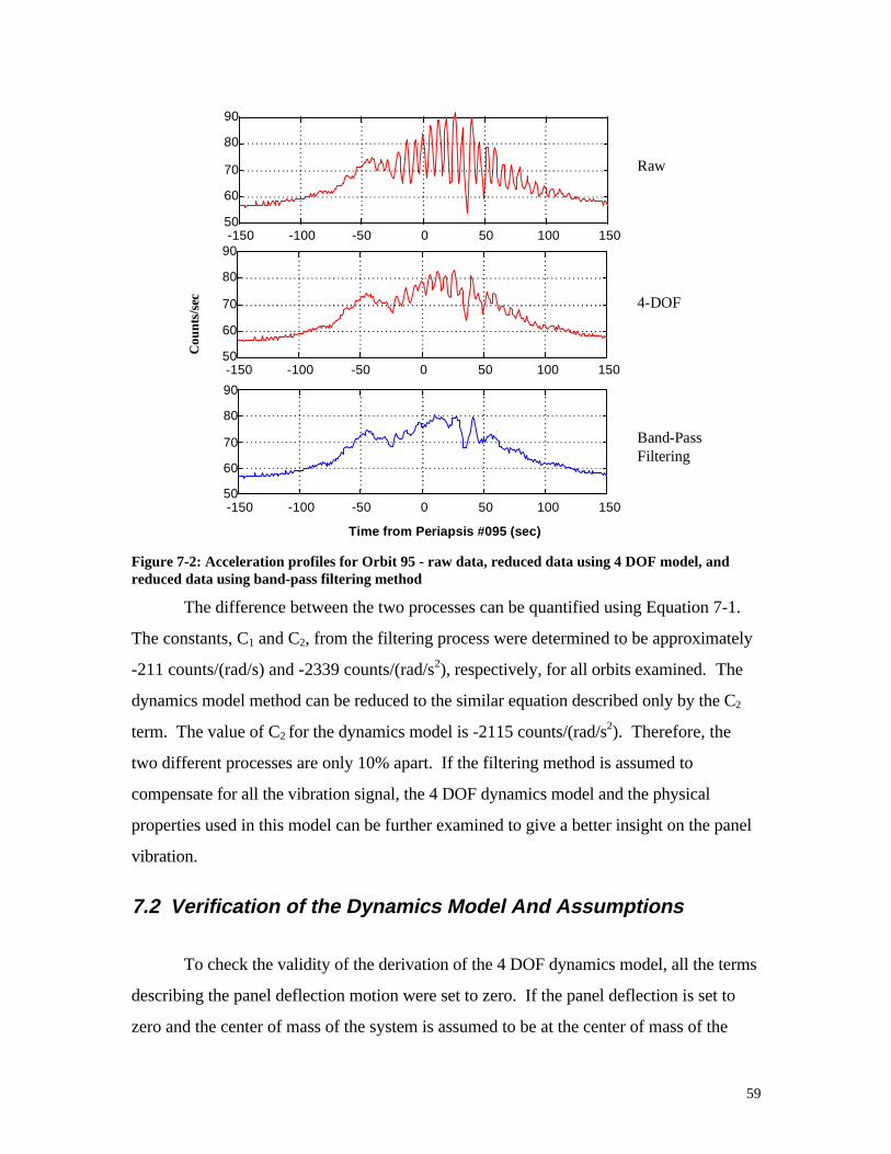
59

-150 -100 -50 0 50 100 15050

60

70

80

90

-150 -100 -50 0 50 100 15050

60

70

80

90

-150 -100 -50 0 50 100 15050

60

70

80

90

Time from Periapsis #095 (sec)

Cou

nts/

sec

Raw

4-DOF

Band-PassFiltering

Figure 7-2: Acceleration profiles for Orbit 95 - raw data, reduced data using 4 DOF model, andreduced data using band-pass filtering method

The difference between the two processes can be quantified using Equation 7-1.

The constants, C1 and C2, from the filtering process were determined to be approximately

-211 counts/(rad/s) and -2339 counts/(rad/s2), respectively, for all orbits examined. The

dynamics model method can be reduced to the similar equation described only by the C2

term. The value of C2 for the dynamics model is -2115 counts/(rad/s2). Therefore, the

two different processes are only 10% apart. If the filtering method is assumed to

compensate for all the vibration signal, the 4 DOF dynamics model and the physical

properties used in this model can be further examined to give a better insight on the panel

vibration.

7.2 Verification of the Dynamics Model And Assumptions

To check the validity of the derivation of the 4 DOF dynamics model, all the terms

describing the panel deflection motion were set to zero. If the panel deflection is set to

zero and the center of mass of the system is assumed to be at the center of mass of the

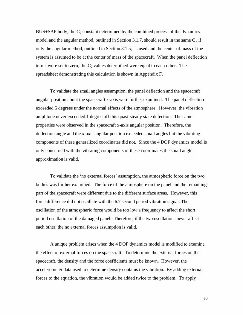
60

BUS+SAP body, the C2 constant determined by the combined process of the dynamics

model and the angular method, outlined in Section 3.1.7, should result in the same C2 if

only the angular method, outlined in Section 3.1.5, is used and the center of mass of the

system is assumed to be at the center of mass of the spacecraft. When the panel deflection

terms were set to zero, the C2 values determined were equal to each other. The

spreadsheet demonstrating this calculation is shown in Appendix F.

To validate the small angles assumption, the panel deflection and the spacecraft

angular position about the spacecraft x-axis were further examined. The panel deflection

exceeded 5 degrees under the normal effects of the atmosphere. However, the vibration

amplitude never exceeded 1 degree off this quasi-steady state defection. The same

properties were observed in the spacecraft x-axis angular position. Therefore, the

deflection angle and the x-axis angular position exceeded small angles but the vibrating

components of these generalized coordinates did not. Since the 4 DOF dynamics model is

only concerned with the vibrating components of these coordinates the small angle

approximation is valid.

To validate the ‘no external forces’ assumption, the atmospheric force on the two

bodies was further examined. The force of the atmosphere on the panel and the remaining

part of the spacecraft were different due to the different surface areas. However, this

force difference did not oscillate with the 6.7 second period vibration signal. The

oscillation of the atmospheric force would be too low a frequency to affect the short

period oscillation of the damaged panel. Therefore, if the two oscillations never affect

each other, the no external forces assumption is valid.

A unique problem arises when the 4 DOF dynamics model is modified to examine

the effect of external forces on the spacecraft. To determine the external forces on the

spacecraft, the density and the force coefficients must be known. However, the

accelerometer data used to determine density contains the vibration. By adding external

forces to the equation, the vibration would be added twice to the problem. To apply

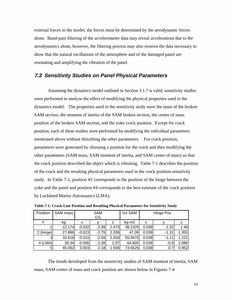
61

external forces to the model, the forces must be determined by the aerodynamic forces

alone. Band-pass filtering of the accelerometer data may reveal accelerations due to the

aerodynamics alone, however, the filtering process may also remove the data necessary to

show that the natural oscillations of the atmosphere and of the damaged panel are

resonating and amplifying the vibration of the panel.

7.3 Sensitivity Studies on Panel Physical Parameters

Assuming the dynamics model outlined in Section 3.1.7 is valid, sensitivity studies

were performed to analyze the effect of modifying the physical properties used in the

dynamics model. The properties used in the sensitivity study were the mass of the broken

SAM section, the moment of inertia of the SAM broken section, the center of mass

position of the broken SAM section, and the yoke crack position. Except for crack

position, each of these studies were performed by modifying the individual parameters

mentioned above without disturbing the other parameters. For crack position,

parameters were generated by choosing a position for the crack and then modifying the

other parameters (SAM mass, SAM moment of inertia, and SAM center of mass) so that

the crack position described the object which is vibrating. Table 7-1 describes the position

of the crack and the resulting physical parameters used in the crack position sensitivity

study. In Table 7-1, position #2 corresponds to the position of the hinge between the

yoke and the panel and position #4 corresponds to the best estimate of the crack position

by Lockheed Martin Astronautics (LMA).

Table 7-1: Crack-Line Position and Resulting Physical Parameters for Sensitivity Study

Position SAM mass SAMCG

Ixx SAM Hinge Pos

# kg x y z kg-m2 x y z1 22.174 -0.032 -2.99 2.473 38.2325 0.038 -1.52 1.49

2 (hinge) 27.896 -0.023 -2.79 2.339 47.09 0.038 -1.31 1.3553 33.618 -0.015 -2.59 2.204 55.9475 0.038 -1.11 1.221

4 (LMA) 39.34 -0.006 -2.39 2.07 64.805 0.038 -0.9 1.0865 45.062 0.003 -2.18 1.936 73.6625 0.038 -0.7 0.952

The trends developed from the sensitivity studies of SAM moment of inertia, SAM

mass, SAM center of mass and crack position are shown below in Figures 7-4

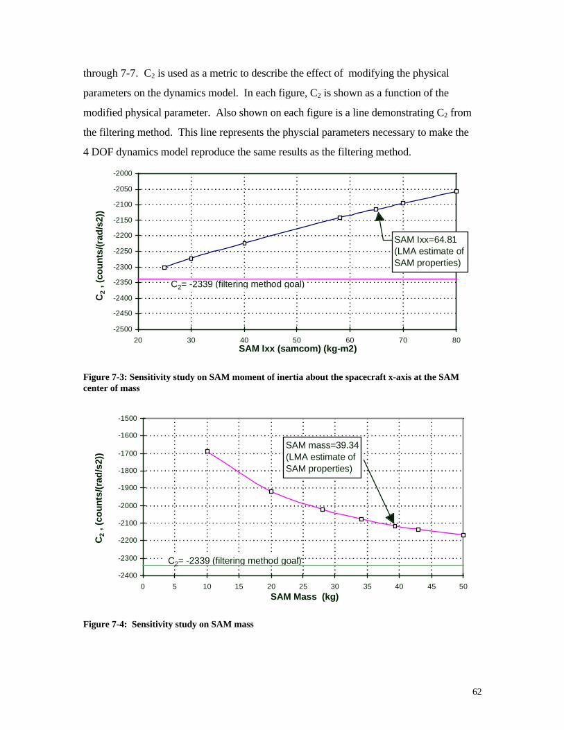
62

through 7-7. C2 is used as a metric to describe the effect of modifying the physical

parameters on the dynamics model. In each figure, C2 is shown as a function of the

modified physical parameter. Also shown on each figure is a line demonstrating C2 from

the filtering method. This line represents the physcial parameters necessary to make the

4 DOF dynamics model reproduce the same results as the filtering method.

-2500

-2450

-2400

-2350

-2300

-2250

-2200

-2150

-2100

-2050

-2000

20 30 40 50 60 70 80SAM Ixx (samcom) (kg-m2)

C2

, (co

unts

/(rad

/s2)

)

C2= -2339 (filtering method goal)

SAM Ixx=64.81 (LMA estimate of SAM properties)

Figure 7-3: Sensitivity study on SAM moment of inertia about the spacecraft x-axis at the SAMcenter of mass

-2400

-2300

-2200

-2100

-2000

-1900

-1800

-1700

-1600

-1500

0 5 10 15 20 25 30 35 40 45 50

SAM Mass (kg)

SAM mass=39.34(LMA estimate ofSAM properties)

C2

, (co

unts

/(rad

/s2)

)

C2= -2339 (filtering method goal)

Figure 7-4: Sensitivity study on SAM mass

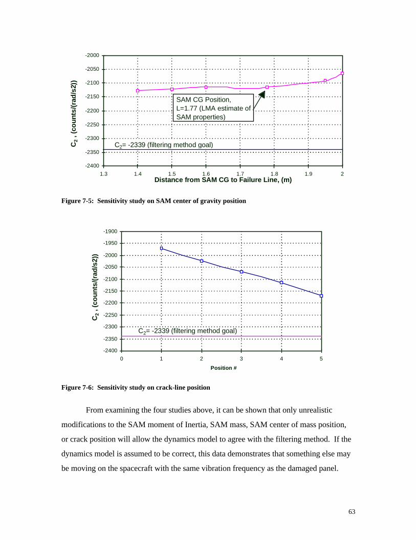
63

-2400

-2350

-2300

-2250

-2200

-2150

-2100

-2050

-2000

1.3 1.4 1.5 1.6 1.7 1.8 1.9 2Distance from SAM CG to Failure Line, (m)

SAM CG Position, L=1.77 (LMA estimate of SAM properties)

C2

, (co

unts

/(rad

/s2)

)

C2= -2339 (filtering method goal)

Figure 7-5: Sensitivity study on SAM center of gravity position

C2

, (co

unts

/(rad

/s2)

)

C2= -2339 (filtering method goal)

-2400

-2350

-2300

-2250

-2200

-2150

-2100

-2050

-2000

-1950

-1900

0 1 2 3 4 5

Position #

Figure 7-6: Sensitivity study on crack-line position

From examining the four studies above, it can be shown that only unrealistic

modifications to the SAM moment of Inertia, SAM mass, SAM center of mass position,

or crack position will allow the dynamics model to agree with the filtering method. If the

dynamics model is assumed to be correct, this data demonstrates that something else may

be moving on the spacecraft with the same vibration frequency as the damaged panel.

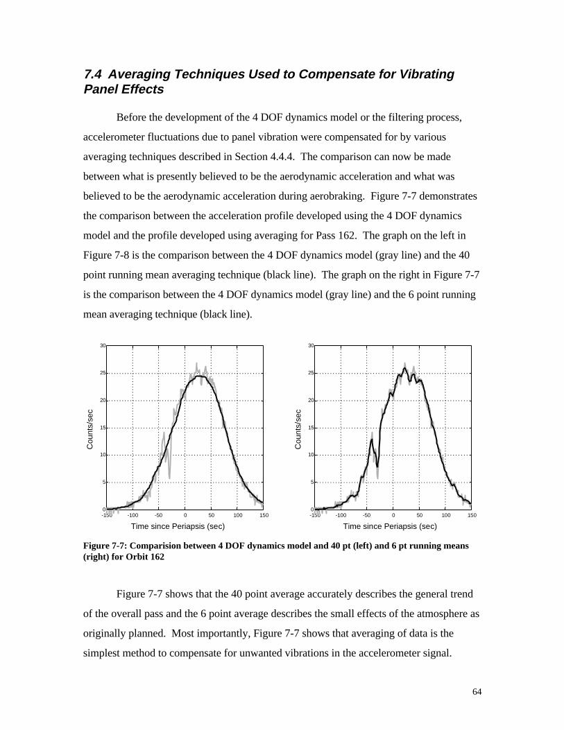
64

7.4 Averaging Techniques Used to Compensate for VibratingPanel Effects

Before the development of the 4 DOF dynamics model or the filtering process,

accelerometer fluctuations due to panel vibration were compensated for by various

averaging techniques described in Section 4.4.4. The comparison can now be made

between what is presently believed to be the aerodynamic acceleration and what was

believed to be the aerodynamic acceleration during aerobraking. Figure 7-7 demonstrates

the comparison between the acceleration profile developed using the 4 DOF dynamics

model and the profile developed using averaging for Pass 162. The graph on the left in

Figure 7-8 is the comparison between the 4 DOF dynamics model (gray line) and the 40

point running mean averaging technique (black line). The graph on the right in Figure 7-7

is the comparison between the 4 DOF dynamics model (gray line) and the 6 point running

mean averaging technique (black line).

-150 -100 -50 0 50 100 1500

5

10

15

20

25

30

Time since Periapsis (sec)

Cou

nts/

sec

-150 -100 -50 0 50 100 1500

5

10

15

20

25

30

Cou

nts/

sec

Time since Periapsis (sec)

Figure 7-7: Comparision between 4 DOF dynamics model and 40 pt (left) and 6 pt running means(right) for Orbit 162

Figure 7-7 shows that the 40 point average accurately describes the general trend

of the overall pass and the 6 point average describes the small effects of the atmosphere as

originally planned. Most importantly, Figure 7-7 shows that averaging of data is the

simplest method to compensate for unwanted vibrations in the accelerometer signal.

65

8. Conclusions

Aerobraking is a low-cost technique which was employed during the MGS mission

and will be used on many upcoming missions. To effectively aerobrake, the density which

the spacecraft encounters on every aerobraking pass must be known. No accurate density

models had been created for the Martian atmosphere at the time of MGS, therefore, the

MGS project was dependent on densities estimated by operational methods to plan the

altitudes at which aerobraking would occur. Aerobraking at Mars was made even more

complex and risky by the malfunction of one of the two solar arrays during initial

deployment.

The MGS Accelerometer Team, formed at George Washington University, used an

operational data reduction procedure to estimate densities given acceleration data from an

on-board accelerometer instrument. This paper has described the operational data

reduction procedure and has also described two methods used to predict the densities of

upcoming orbits. These density estimations and predictions formed the basis for the

planning of aerobraking altitudes during the first 201 orbits of MGS aerobraking. In

addition, the operational data reduction procedure has provided the density data necessary

for 1) the discovery of two longitudinal density bulges on opposite sides of Mars and 2)

the first record of the effects of a dust storm on the density of the Martian neutral upper

atmosphere.

The operational data reduction procedure was developed around an iterative

process which determines density by calculating the deflection of the damaged solar array

and a variable force coefficient which accounts for aerodynamic flight regime, spacecraft

orientation and solar array deflection. This procedure has been demonstrated to determine

densities up to 33 km above periapsis in 7 minutes (approximately 1/20th of 2 hour time

period allotted for MGS operational density analysis). The possible errors over this

altitude range were determined to be less than 5% by considering the total density

66

error from ephemeris errors, errors in force coefficient and instrument errors. The

accuracy of this procedure has also been verified by comparing the solar array deflection

and orbital period reduction calculated by this procedure to independent calculations

performed by other MGS Teams including the Navigation and Spacecraft Teams.

The damaged solar array deflected and vibrated each pass through the atmosphere,

producing an oscillating signal in the accelerometer data. To analyze and remove this

signal, three methods were developed: averaging, band-pass filtering and a 4 degree of

freedom dynamics model. By using the averaging method, the analysis of accelerometer

data was not affected by this vibration. By comparing the remaining two methods

developed to analyze the vibration signal, a greater understanding of the dynamics of the

panel and the spacecraft was established. The 4 degree of freedom model successfully

compensated for 90% of vibration signal determined by the filtering process. Sensitivity

studies, performed to determine the source of the outstanding 10%, revealed that the

remaining signal may be due to external forces not represented in the model or another

component on the spacecraft moving at the same vibration frequency such as fuel sloshing.

67

References

[1]- “Mars Global Surveyor Fact Sheet”, Jet Propulsion Laboratory Publication, JPL 410-44-2, Dec 1994.

[2]- Dallas, S. Sam, “Mars Global Surveyor Mission.” Presented at the 1997 IEEEAerospace Conference, Snowmass at Aspen, CO, 1997. Vol. 4, pp173-189.

[3]- Lyons, D.T., “Aerobraking Magellan: Plan Versus Reality,” AAS-94-118, 1994.

[4]- Tolson, R.H., et al., “Magellan Windmill and Termination Experiments,” SpaceflightDynamics, CNES June 1995 Conference, Toulouse, France.

[5]- Keating, G.M. et al., “Models of Venus Neutral Upper Atmosphere: Structure andComposition,” Adv. Space Res. Vol. 5, No. 11, 1985 pp 117-171.

[5]- Shane, R.W. and Tolson, R.H., “Aerothermodynamics of the Mars Global SurveyorSpacecraft,” NASA/ CR-1998-206941, March 1998.

[7]- Wilmoth, R.G. et al., “Rarefied Aerothermodymanic Predictions for Mars GlobalSurveyor,” To be published in the Journal of Spacecraft and Rockets.

[8]- Kahn, R. et. al., Mars, H.H. Kieffer, B.M. Jakosky, C.W. Synder, M.S. Matthews,Eds., Univ. of Arizona Press, Tucson, 1992. Pp 1017-1053. Martin, L.J. and Zurek,R.W., Journal of Geophysical Research, 97, 3221, 1993.

[9]- Lyons, D. T. et al., “Mars Global Surveyor: Aerobraking Mission Overview.” To bepublished in the Journal of Spacecraft and Rockets.

[10]- Diamond, P.S. and Tolson, R.H., “A Feasibility Study of a MicrogravityEnhancement System for Space Station Freedom.” AAS Paper 93-626, August1993.

[11]- Larson, W. J. and Wertz, J.R., Space Mission Analysis and Design, Microcosm Inc,CA, 1992.

[12]- Meirovitch, L., Methods of Analytical Dynamics, McGraw-Hill Inc., 1970.

[13]- Cestero, F.J. and Tolson, R.H., “Magellan Aerodynamic Characteristics During theTermination Experiment Including Thruster Plume-Free Stream Interaction.”NASA/CR-1998-206940, March 1998.

[14]- Henderson, D. M., “Euler Angles, Quaternions, and Transformation Matricies –Working Relationships,” NASA TM-74839, JSC-12960, July 1977.

68

[15]- Blanchard, R.C. and Walberg, G.D.. “Determination of the Hypersonic-Continuum/Rarefied-Flow Drag Coefficient of the Viking Lander Capsule 1 Aeroshellfrom Flight Data.” NASA Technical Paper 1793, Dec 1980.

[16]- Keating G.M., Cancro G. J., et al., “The Structure of the Upper Atmopshere ofMars: In-Situ Accelerometer Measurements from Mars Global Surveyor,” Science,Vol. 279, March 13, 1998, pp 1672-1676.

[17]- King-Hele, D., “Satellite Orbits in an Atmosphere: Theory and Applications,”Blackie and Sons, Ltd, 1987.

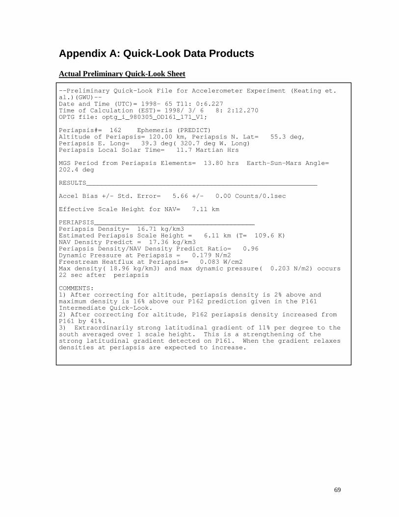
69

Appendix A: Quick-Look Data Products

Actual Preliminary Quick-Look Sheet

--Preliminary Quick-Look File for Accelerometer Experiment (Keating et.al.)(GWU)--Date and Time (UTC)= 1998- 65 T11: 0:6.227Time of Calculation (EST)= 1998/ 3/ 6 8: 2:12.270OPTG file: optg_i_980305_OD161_171_V1;

Periapsis#= 162 Ephemeris (PREDICT)Altitude of Periapsis= 120.00 km, Periapsis N. Lat= 55.3 deg,Periapsis E. Long= 39.3 deg( 320.7 deg W. Long)Periapsis Local Solar Time= 11.7 Martian Hrs

MGS Period from Periapsis Elements= 13.80 hrs Earth-Sun-Mars Angle=202.4 deg

RESULTS___________________________________________________________

Accel Bias +/- Std. Error= 5.66 +/- 0.00 Counts/0.1sec

Effective Scale Height for NAV= 7.11 km

PERIAPSIS_________________________________________Periapsis Density= 16.71 kg/km3Estimated Periapsis Scale Height = 6.11 km (T= 109.6 K)NAV Density Predict = 17.36 kg/km3Periapsis Density/NAV Density Predict Ratio= 0.96Dynamic Pressure at Periapsis = 0.179 N/m2Freestream Heatflux at Periapsis= 0.083 W/cm2Max density( 18.96 kg/km3) and max dynamic pressure( 0.203 N/m2) occurs22 sec after periapsis

COMMENTS:1) After correcting for altitude, periapsis density is 2% above andmaximum density is 16% above our P162 prediction given in the P161Intermediate Quick-Look.2) After correcting for altitude, P162 periapsis density increased fromP161 by 41%.3) Extraordinarily strong latitudinal gradient of 11% per degree to thesouth averaged over 1 scale height. This is a strengthening of thestrong latitudinal gradient detected on P161. When the gradient relaxesdensities at periapsis are expected to increase.

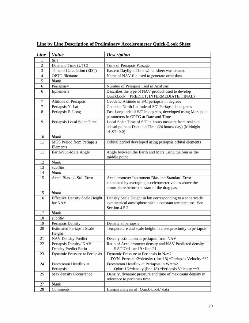
70

Line by Line Description of Preliminary Accelerometer Quick-Look Sheet

Line Value Description1 title2 Date and Time (UTC) Time of Periapsis Passage3 Time of Calculation (EDT) Eastern Daylight Time which sheet was created4 OPTG filename Name of NAV file used to generate orbit data5 blank6 Periapsis# Number of Periapsis used in Analysis6 Ephemeris Describes the type of NAV product used to develop

QuickLook: (PREDICT, INTERMEDIATE, FINAL)7 Altitude of Periapsis Geodetic Altitude of S/C periapsis in degrees7 Periapsis N. Lat Geodetic North Latitude of S/C Periapsis in degrees8 Periapsis E. Long East Longitude of S/C in degrees, developed using Mars pole

parameters in OPTG at Date and Time9 Periapsis Local Solar Time Local Solar Time of S/C in hours measure from real sun

subsol point at Date and Time (24 hours/ day) (Midnight ->LST=0.0)

10 blank11 MGS Period from Periapsis

ElementsOrbital period developed using periapsis orbital elements

11 Earth-Sun-Mars Angle Angle between the Earth and Mars using the Sun as themiddle point

12 blank13 subtitle14 blank15 Accel Bias +/- Std. Error Accelerometer Instrument Bias and Standard Error

calculated by averaging accelerometer values above theatmosphere before the start of the drag pass

15 blank16 Effective Density Scale Height

for NAVDensity Scale Height in km corresponding to a sphericallysymmetrical atmosphere with a constant temperature. SeeSection 4.5.2

17 blank18 subtitle19 Periapsis Density Density at periapsis20 Estimated Periapsis Scale

HeightTemperature and scale height in close proximity to periapsis

21 NAV Density Predict Density estimation at periapsis from NAV22 Periapsis Density/ NAV

Density Predict RatioRatio of Accelerometer density and NAV Predicted density RATIO=Line 19 / line 21

23 Dynamic Pressure at Periapsis Dynamic Pressure at Periapsis in N/m2 DYN. Press.=1/2*density (line 18) *Periapsis Velocity.**2

24 Freestream Heatflux atPeriapsis

Freestream Heatflux at Periapsis in W/cm2 Qdot=1/2*density (line 18) *Periapsis Velcoity.**3

25 Max density Occurrence Density, dynamic pressure and time of maximum density inreference to periapsis time

27 blank28 Comments Human analysis of ‘Quick-Look’ data

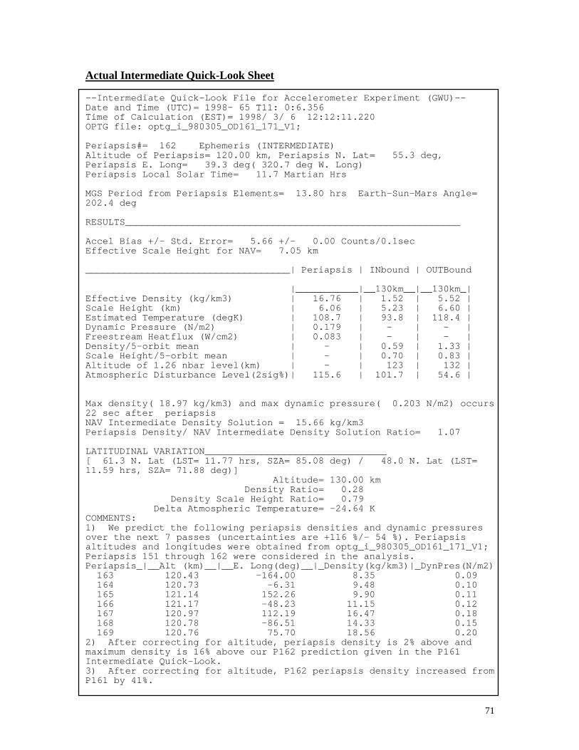
71

Actual Intermediate Quick-Look Sheet

--Intermediate Quick-Look File for Accelerometer Experiment (GWU)--Date and Time (UTC)= 1998- 65 T11: 0:6.356Time of Calculation (EST)= 1998/ 3/ 6 12:12:11.220OPTG file: optg_i_980305_OD161_171_V1;

Periapsis#= 162 Ephemeris (INTERMEDIATE)Altitude of Periapsis= 120.00 km, Periapsis N. Lat= 55.3 deg,Periapsis E. Long= 39.3 deg( 320.7 deg W. Long)Periapsis Local Solar Time= 11.7 Martian Hrs

MGS Period from Periapsis Elements= 13.80 hrs Earth-Sun-Mars Angle=202.4 deg

RESULTS___________________________________________________________

Accel Bias +/- Std. Error= 5.66 +/- 0.00 Counts/0.1secEffective Scale Height for NAV= 7.05 km

____________________________________| Periapsis | INbound | OUTBound

|___________|__130km__|__130km_|Effective Density (kg/km3) | 16.76 | 1.52 | 5.52 |Scale Height (km) | 6.06 | 5.23 | 6.60 |Estimated Temperature (degK) | 108.7 | 93.8 | 118.4 |Dynamic Pressure (N/m2) | 0.179 | - | - |Freestream Heatflux (W/cm2) | 0.083 | - | - |Density/5-orbit mean | - | 0.59 | 1.33 |Scale Height/5-orbit mean | - | 0.70 | 0.83 |Altitude of 1.26 nbar level(km) | - | 123 | 132 |Atmospheric Disturbance Level(2sig%)| 115.6 | 101.7 | 54.6 |

Max density( 18.97 kg/km3) and max dynamic pressure( 0.203 N/m2) occurs22 sec after periapsisNAV Intermediate Density Solution = 15.66 kg/km3Periapsis Density/ NAV Intermediate Density Solution Ratio= 1.07

LATITUDINAL VARIATION________________________________[ 61.3 N. Lat (LST= 11.77 hrs, SZA= 85.08 deg) / 48.0 N. Lat (LST=11.59 hrs, SZA= 71.88 deg)]

Altitude= 130.00 km Density Ratio= 0.28 Density Scale Height Ratio= 0.79 Delta Atmospheric Temperature= -24.64 K

COMMENTS:1) We predict the following periapsis densities and dynamic pressuresover the next 7 passes (uncertainties are +116 %/- 54 %). Periapsisaltitudes and longitudes were obtained from optg_i_980305_OD161_171_V1;Periapsis 151 through 162 were considered in the analysis.Periapsis_|__Alt (km)__|__E. Long(deg)__|_Density(kg/km3)|_DynPres(N/m2) 163 120.43 -164.00 8.35 0.09 164 120.73 -6.31 9.48 0.10 165 121.14 152.26 9.90 0.11 166 121.17 -48.23 11.15 0.12 167 120.97 112.19 16.47 0.18 168 120.78 -86.51 14.33 0.15 169 120.76 75.70 18.56 0.202) After correcting for altitude, periapsis density is 2% above andmaximum density is 16% above our P162 prediction given in the P161Intermediate Quick-Look.3) After correcting for altitude, P162 periapsis density increased fromP161 by 41%.

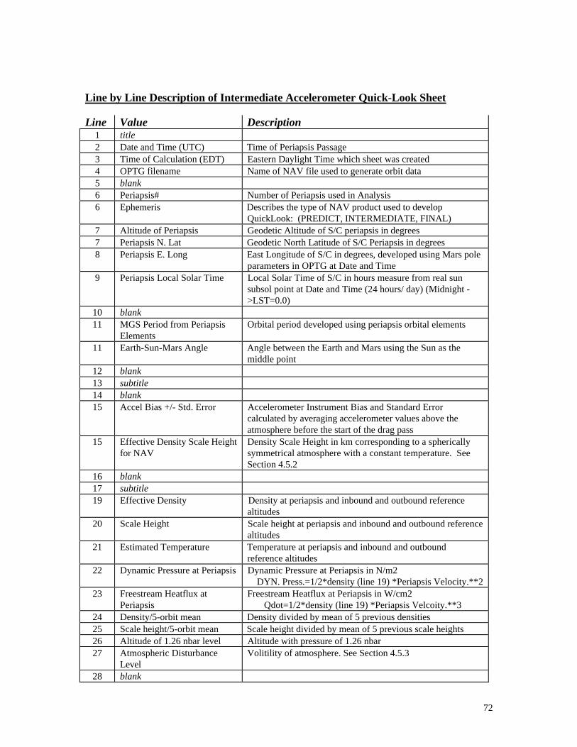
72

Line by Line Description of Intermediate Accelerometer Quick-Look Sheet

Line Value Description1 title2 Date and Time (UTC) Time of Periapsis Passage3 Time of Calculation (EDT) Eastern Daylight Time which sheet was created4 OPTG filename Name of NAV file used to generate orbit data5 blank6 Periapsis# Number of Periapsis used in Analysis6 Ephemeris Describes the type of NAV product used to develop

QuickLook: (PREDICT, INTERMEDIATE, FINAL)7 Altitude of Periapsis Geodetic Altitude of S/C periapsis in degrees7 Periapsis N. Lat Geodetic North Latitude of S/C Periapsis in degrees8 Periapsis E. Long East Longitude of S/C in degrees, developed using Mars pole

parameters in OPTG at Date and Time9 Periapsis Local Solar Time Local Solar Time of S/C in hours measure from real sun

subsol point at Date and Time (24 hours/ day) (Midnight ->LST=0.0)

10 blank11 MGS Period from Periapsis

ElementsOrbital period developed using periapsis orbital elements

11 Earth-Sun-Mars Angle Angle between the Earth and Mars using the Sun as themiddle point

12 blank13 subtitle14 blank15 Accel Bias +/- Std. Error Accelerometer Instrument Bias and Standard Error

calculated by averaging accelerometer values above theatmosphere before the start of the drag pass

15 Effective Density Scale Heightfor NAV

Density Scale Height in km corresponding to a sphericallysymmetrical atmosphere with a constant temperature. SeeSection 4.5.2

16 blank17 subtitle19 Effective Density Density at periapsis and inbound and outbound reference

altitudes20 Scale Height Scale height at periapsis and inbound and outbound reference

altitudes21 Estimated Temperature Temperature at periapsis and inbound and outbound

reference altitudes22 Dynamic Pressure at Periapsis Dynamic Pressure at Periapsis in N/m2

DYN. Press.=1/2*density (line 19) *Periapsis Velocity.**223 Freestream Heatflux at

PeriapsisFreestream Heatflux at Periapsis in W/cm2 Qdot=1/2*density (line 19) *Periapsis Velcoity.**3

24 Density/5-orbit mean Density divided by mean of 5 previous densities25 Scale height/5-orbit mean Scale height divided by mean of 5 previous scale heights26 Altitude of 1.26 nbar level Altitude with pressure of 1.26 nbar27 Atmospheric Disturbance

LevelVolitility of atmosphere. See Section 4.5.3

28 blank

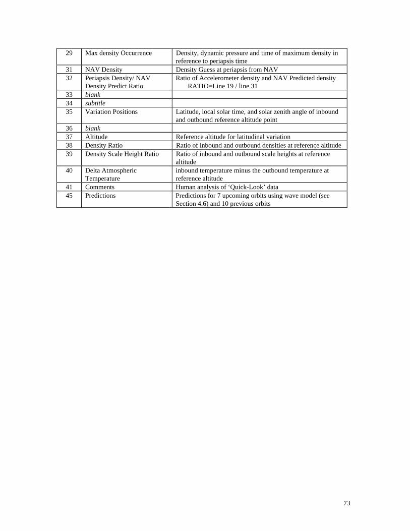
73

29 Max density Occurrence Density, dynamic pressure and time of maximum density inreference to periapsis time

31 NAV Density Density Guess at periapsis from NAV32 Periapsis Density/ NAV

Density Predict RatioRatio of Accelerometer density and NAV Predicted density RATIO=Line 19 / line 31

33 blank34 subtitle35 Variation Positions Latitude, local solar time, and solar zenith angle of inbound

and outbound reference altitude point36 blank37 Altitude Reference altitude for latitudinal variation38 Density Ratio Ratio of inbound and outbound densities at reference altitude39 Density Scale Height Ratio Ratio of inbound and outbound scale heights at reference

altitude40 Delta Atmospheric

Temperatureinbound temperature minus the outbound temperature atreference altitude

41 Comments Human analysis of ‘Quick-Look’ data45 Predictions Predictions for 7 upcoming orbits using wave model (see

Section 4.6) and 10 previous orbits

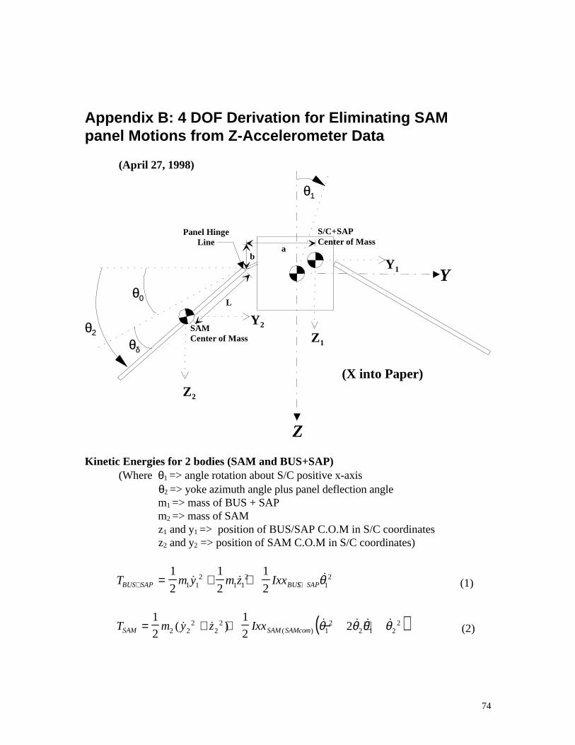
74

Appendix B: 4 DOF Derivation for Eliminating SAMpanel Motions from Z-Accelerometer Data

(April 27, 1998)

Y

Z

Z1

Z2

Y1

Y2

θ0

θδ

θ1

Panel Hinge Line

S/C+SAP Center of Mass

SAM Center of Mass

ab

θ2

(X into Paper)

L

Kinetic Energies for 2 bodies (SAM and BUS+SAP)(Where θ1 => angle rotation about S/C positive x-axis

θ2 => yoke azimuth angle plus panel deflection angle m1 => mass of BUS + SAP m2 => mass of SAM z1 and y1 => position of BUS/SAP C.O.M in S/C coordinates z2 and y2 => position of SAM C.O.M in S/C coordinates)

T m y m z IxxBUS SAP BUS SAP+ += + +1

2

1

2

1

21 12

1 12

12

θ (1)

( )T m y z IxxSAM SAM SAMcom= + + − +1

2

1

222 2

22

21

22 1 2

2( ) ( ) θ θ θ θ (2)

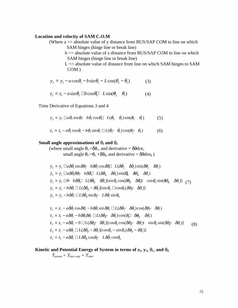
75

Location and velocity of SAM C.O.M(Where a => absolute value of y distance from BUS/SAP COM to line on which

SAM hinges (hinge line or break line)b => absolute value of z distance from BUS/SAP COM to line on which SAM hinges (hinge line or break line)L => absolute value of distance from line on which SAM hinges to SAM COM )

y y a b L2 1 1 1 2 1= − − − −cos sin cos( )θ θ θ θ (3)

z z a b L2 1 1 1 2 1= − + + −sin cos sin( )θ θ θ θ (4)

Time Derivative of Equations 3 and 4

sin cos ( )sin( )y y a b L2 1 1 1 1 1 2 1 2 1= + − + − −θ θ θ θ θ θ θ θ (5)

cos sin ( )cos( )z z a b L2 1 1 1 1 1 2 1 2 1= − − + − −θ θ θ θ θ θ θ θ (6)

Small angle approximations of θ1 and θ2

(where small angle θ1 =δθ1, and derivative = δθdot1small angle θ2 =θo +δθδ, and derivative = δθdotδ )

sin cos ( )sin( )

( )sin( )

( )[sin cos( ) cos sin( )]

y y a b L

y y a b L

y y b L

y y b

2 1 1 1 1 1 2 1 2 1

2 1 1 1 1 1 0 1

2 1 1 1 0 1 0 1

2 1 1

0

≈ + − + − −

≈ + − + − + −

≈ + − + − − + −

≈ − +

δθ δθ δθ δθ δθ δθ δθ δθ

δθ δθ δθ δθ δθ θ δθ δθ

δθ δθ δθ θ δθ δθ θ δθ δθ

δθ

δ δ

δ δ δ

L

y y b L L

( )[sin cos ( )]

sin sin

δθ δθ θ θ δθ δθ

δθ δθ θ δθ θδ δ

δ

− + −

= − + −1 0 0 1

2 1 1 0 1 0

(7)

cos sin ( )cos( )

( )cos( )

( )[cos cos( ) sin sin( )]

z z a b L

z z a b L

z z a L

z z a

2 1 1 1 1 1 2 1 2 1

2 1 1 1 1 1 0 1

2 1 1 1 0 1 0 1

2 1 1

0

= − − + − −

= − − + − + −

= − − + − − − −

= − +

δθ δθ δθ δθ δθ δθ δθ δθ

δθ δθ δθ δθ δθ θ δθ δθ

δθ δθ δθ θ δθ δθ θ δθ δθ

δθ

δ δ

δ δ δ

L

z z a L L

( )[cos sin ( )]

cos cos

δθ δθ θ θ δθ δθ

δθ δθ θ δθ θδ δ

δ

− − −

= − + −1 0 0 1

2 1 1 0 1 0

(8)

Kinetic and Potential Energy of System in terms of z1, y1, θ1, and θδ

Τsystem = Tbus+sap + Tsam

76

( )T m y z Ixx m y z

Ixx

system BUS SAP

SAM SAMcom

= + + + +

+ − +

+

1

2

1

2

1

21

22

1 12

12

12

2 22

22

12

12

( ) ( )

( )

δθ

δθ δθ δθ δθδ δ

(9)

V Md T dX

Tsystem CX

eC

Xe e= = =+∫ ∫ +θ θ θ θδ( )

1

11 (10)

L=T-V,

After forming the lagrangian, the z1, y1, θ1 coordinates are found to be cyclic and thekinetic energy is a homogenous polynomial of degree 2, therefore the momentum inz1, y1, θ1 is time independent (derivative equals zero)

d

dt

L

y

∂∂1

0

=

d

dt

L

z

∂∂1

0

=

d

dt

L∂∂θ1

0

= (11)

For corresponding momentum in y1 :

∂∂

∂∂

L

ym y m y

y

y

11 1 2 2

2

1

= + where sin siny y b L L2 1 1 0 1 0= − + −δθ δθ θ δθ θδ

and ∂∂

y

y2

1

1=

therefore ( )∂∂

δθ δθ θ δθ θδ

L

ym y m y b L L

sin sin

11 1 2 1 1 0 1 0= + − + −

( )d

dt

L

zm y m y b L L

∂∂ δθ δθ θ δθ θδ

sin sin

11 1 2 1 1 0 1 0 0

= + − + − = (12)

For corresponding momentum in z1 :

∂∂

∂∂

L

zm z m z

z

z

11 1 2 2

2

1

= + where cos cosz z a L L2 1 1 0 1 0= − + −δθ δθ θ δθ θδ

and ∂∂

z

z2

1

1=

therefore ( )∂∂

δθ δθ θ δθ θδ

L

zm z m z a L L

cos cos

11 1 2 1 1 0 1 0= + − + −

( )d

dt

L

zm z m z a L L

∂∂

δθ δθ θ δθ θδ

cos cos1

1 1 2 1 1 0 1 0 0

= + − + − = (13)

77

For corresponding momentum in θ1 :

( )∂∂ δθ

∂∂ δθ

∂∂ δθ

δθ δθ δθδ

Lm z

zm y

yIxx IxxBUS SAP SAM SAMcom

( )1

2 22

12 2

2

11 1= + + + −+

where∂∂δθ

θ

sin

yb L2

10= − − and

∂∂δθ

θ

cos

za L2

10= − −

therefore ∂∂ δθ

δθ δθ θ δθ θ θ

δθ δθ θ δθ θ θ

δθ δθ δθ

δ

δ

δ

Lm z a L L a L

m y b L L b L

Ixx IxxBUS SAP SAM SAMcom

( cos cos )( cos )

( sin sin )( sin ) ( )( )

12 1 1 0 1 0 0

2 1 1 0 1 0 0

1 1

= − + − − −

+ − + − − −

+ + −+

∂∂ δθ

θ δθ θ θ

δθ θ θ θ

δθ θ θ δθ θ θ

δθ

δ

δ

Lz m a m L m a m aL m L

m aL m L y m b m L

m b m bL m L m bL m L

Ixx

( cos ) ( cos cos )

( cos cos ) ( sin ) ( sin sin ) ( sin sin ) (

11 2 2 0 1 2

22 0 2

2 20

2 0 22 2

0 1 2 2 0

1 22

2 0 22 2

0 2 0 22 2

0

1

2

2

= − − + + +

+ − − + − − +

+ + + + − −

+ BUS SAP SAM SAMcom SAM SAMcomIxx Ixx+ + −( ) ( )) ( )δθδ

∂∂ δθ

θ θ

δθ θ θ

δθ θ θδ

Lz ma m L y mb m L

maL m L mbL Ixx

ma maL m L mb mbL Ixx Ixx

SAM SAMcom

BUS SAP SAM SAMcom

( cos ) ( sin )

( cos sin )

( cos sin )

( )

( )

11 2 2 0 1 2 2 0

2 0 22

2 0

1 22

2 0 22

22

2 02 2

= − − + − −

+ − − − −

+ + + + + + ++

d

dt

Lz ma mL y mb mL

maL mL mbL Ixx

ma maL mL mb mbL Ixx Ixx

SAM SAMcom

BUS SAP SAM SAMcom

∂∂ δθ

θ θ

δθ θ θ

δθ θ θδ

( cos ) ( sin )

( cos sin )

( cos sin )

( )

( )

11 2 2 0 1 2 2 0

2 0 22

2 0

1 22

2 0 22

22

2 02 2 0

= − − + − −

+ − − − −

+ + + + + + + =+

Using the momentum equations, 3 equations are produced with 4 unknowns (y1 z1

θ1 and θδ) . However, θ1 in this problem is known as the S/C x-angular position,which is delivered as x-angular rate data once every sec during the drag pass.This reduces this problem to 3 equations and 3 unknowns that can be solved fordz1/dt every sec which is the change in velocity each second measured by the z-accelerometer due to the motion of the SAM panel if there are no outside forceson the panel and if small angles apply. This data can be removed from the

78

acceleration signal further reducing the false signals read by the instruments dueto S/C motion.

3 Equations used shown below:

( ) ( sin ) ( sin ) m m y m b m L m L1 2 1 2 2 0 1 2 0 0+ + − − + =θ δθ θ δθδ (15)

( ) ( cos ) ( cos ) m m z m a m L m L1 2 1 2 2 0 1 2 0 0+ + − − + =θ δθ θ δθδ (16)

( cos ) ( sin ) ( cos sin )

( cos sin )

( )

( )

z m a m L y m b m L

m aL m L m bL Ixx

m a m aL m L m b m bL Ixx Ixx

SAM SAMcom

BUS SAP SAM SAMcom

1 2 2 0 1 2 2 0

2 0 22

2 0

1 22

2 0 22

22

2 02 2 0

− − + − −

+ − − − −

+ + + + + + + =+

θ θ

δθ θ θ

δθ θ θδ

(17)

These are solved by setting the following constants:a11= m1+m2 a21= 0a12= 0 a22= m1+m2

a13= -m2b-m2Lsinθ0 a23= -m2a-m2Lcosθ0

a14= m2Lsinθ0 a24= m2Lcosθ0

a31= -m2b-m2Lsinθ0

a32= -m2a-m2Lcosθ0

a33= m2a2+2m2aLcosθ0 +m2L

2+m2b2+2m2bLsinθ0+IxxBUS+SAP+IxxSAM(SAMcom)

a34= -m2aLcosθ0 −m2L2-m2bLsinθ0−IxxSAM(SAMcom)

a a a a

a a a a

a a a a

y

za a a

a a a

a a a

y

z

a

a

a

11 12 13 14

21 22 23 24

31 32 33 34

0 0 0 0

0

0

0

0

11 12 14

21 22 24

31 32 34

13

23

33

1

1

1

1

1

=

=−−−

δθδθ δθ

δδ

=

−

−−

=

−

δθ

δθδθ

δθδ δ

1

1

1 1

1

1

1 014

110 22 24

31 32 34

13

1123

33

1 014

11

0 124

2231 32 34

a

aa a

a a a

y

z

a

aa

a

a

aa

aa a a

y

z

a13

1123

2233

1 014

11

0 124

22

0 32 34 3114

11

13

1123

22

33 3113

11

1 014

11

0 124

22

0 0

1

1

1 1

aa

aa

a

aa

a

a a aa

a

y

z

a

aa

a

a aa

a

a

aa

a

−

−

−

=

−

−

− +

δθ

δθδθ

δ

C aa

a

y

z

a

aa

a

C aa

a1

1

1

2

1

3224

22

13

1123

22

3223

22−

=

−

−

+

δθδθ

δ

79

where C1=a34-a31*(a14/a11) and C2= -a33+a31*(a13/a11)C3=C1-a32*(a24/a22) and C4= C2+a32*(a23/a22)

1 014

11

0 124

220 0

13

1123

22

1 014

11

0 124

220 0 1

13

1123

3

1

1

4

1

1

1

a

aa

aC

y

z

a

aa

aC

a

aa

a

y

z

a

aa

=

−

−

=

−

−

δθδθ

δθδ δ

aC

C

a

ay

z

a

aa

a

a

a

C

CC

C

y

z

22

1 014

110 1 0

0 0 1

13

1123

22

24

22

1 0 0

0 1 0

0 0 1

4

3

1

1

14

3

4

3

1

1

1

=

−

−−

δθ

δθδθ

δθδ δ

=

−−

−−

a

a

a

a

C

Ca

a

a

a

C

CC

C

13

11

14

1123

22

24

22

4

3

4

3

4

3

1δθ

80

Appendix C: LaRC Aerothermodynamic Database forMGS Operations

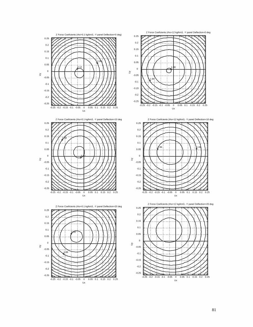
81

-0.25 -0.2 -0.15 -0.1 -0.05 0 0.05 0.1 0.15 0.2 0.25

-0.25

-0.2

-0.15

-0.1

-0.05

0

0.05

0.1

0.15

0.2

0.25

1.94

1.98

Z Force Coeficients (rho=12 kg/km3, -Y panel Deflection=0 deg

Ux

Uy

-0.25 -0.2 -0.15 -0.1 -0.05 0 0.05 0.1 0.15 0.2 0.25

-0.25

-0.2

-0.15

-0.1

-0.05

0

0.05

0.1

0.15

0.2

0.25

1.821.86

Z Force Coeficients (rho=12 kg/km3, -Y panel Deflection=10 deg

Ux

Uy

-0.25 -0.2 -0.15 -0.1 -0.05 0 0.05 0.1 0.15 0.2 0.25

-0.25

-0.2

-0.15

-0.1

-0.05

0

0.05

0.1

0.15

0.2

0.25

Z Force Coeficients (rho=12 kg/km3, -Y panel Deflection=20 deg

Ux

Uy

-0.25 -0.2 -0.15 -0.1 -0.05 0 0.05 0.1 0.15 0.2 0.25

-0.25

-0.2

-0.15

-0.1

-0.05

0

0.05

0.1

0.15

0.2

0.25

2.08

2.12

Z Force Coeficients (rho=0.1 kg/km3, -Y panel Deflection=0 deg)

Ux

Uy

-0.25 -0.2 -0.15 -0.1 -0.05 0 0.05 0.1 0.15 0.2 0.25

1.98

2.02

Z Force Coeficients (rho=0.1 kg/km3, -Y panel Deflection=10 deg

Ux

-0.25

-0.2

-0.15

-0.1

-0.05

0

0.05

0.1

0.15

0.2

0.25

Uy

-0.25 -0.2 -0.15 -0.1 -0.05 0 0.05 0.1 0.15 0.2 0.25

-0.25

-0.2

-0.15

-0.1

-0.05

0

0.05

0.1

0.15

0.2

0.25

1.88

1.92

Z Force Coeficients (rho=0.1 kg/km3, -Y panel Deflection=20 deg

Ux

Uy

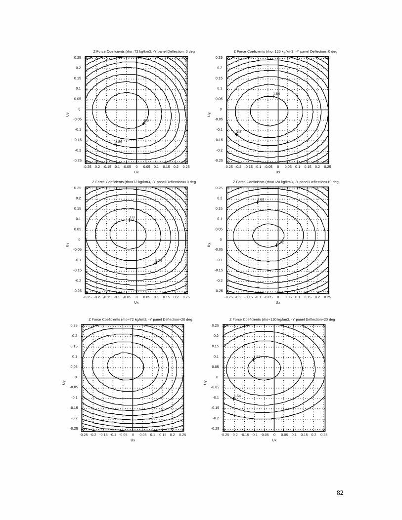
82

-0.25 -0.2 -0.15 -0.1 -0.05 0 0.05 0.1 0.15 0.2 0.25

-0.25

-0.2

-0.15

-0.1

-0.05

0

0.05

0.1

0.15

0.2

0.25

1.86

1.9

Z Force Coeficients (rho=72 kg/km3, -Y panel Deflection=0 deg

Ux

Uy

-0.25 -0.2 -0.15 -0.1 -0.05 0 0.05 0.1 0.15 0.2 0.25

-0.25

-0.2

-0.15

-0.1

-0.05

0

0.05

0.1

0.15

0.2

0.25

1.76

1.8

Z Force Coeficients (rho=72 kg/km3, -Y panel Deflection=10 deg

Ux

Uy

-0.25 -0.2 -0.15 -0.1 -0.05 0 0.05 0.1 0.15 0.2 0.25

-0.25

-0.2

-0.15

-0.1

-0.05

0

0.05

0.1

0.15

0.2

0.25

Z Force Coeficients (rho=72 kg/km3, -Y panel Deflection=20 deg

Ux

Uy

-0.25 -0.2 -0.15 -0.1 -0.05 0 0.05 0.1 0.15 0.2 0.25

-0.25

-0.2

-0.15

-0.1

-0.05

0

0.05

0.1

0.15

0.2

0.25

1.8

1.84

Z Force Coeficients (rho=120 kg/km3, -Y panel Deflection=0 deg

Ux

Uy

-0.25 -0.2 -0.15 -0.1 -0.05 0 0.05 0.1 0.15 0.2 0.25

-0.25

-0.2

-0.15

-0.1

-0.05

0

0.05

0.1

0.15

0.2

0.25

1.68

1.72

Z Force Coeficients (rho=120 kg/km3, -Y panel Deflection=10 deg

Ux

Uy

-0.25 -0.2 -0.15 -0.1 -0.05 0 0.05 0.1 0.15 0.2 0.25

-0.25

-0.2

-0.15

-0.1

-0.05

0

0.05

0.1

0.15

0.2

0.25

1.54

1.58

Z Force Coeficients (rho=120 kg/km3, -Y panel Deflection=20 deg

Ux

Uy

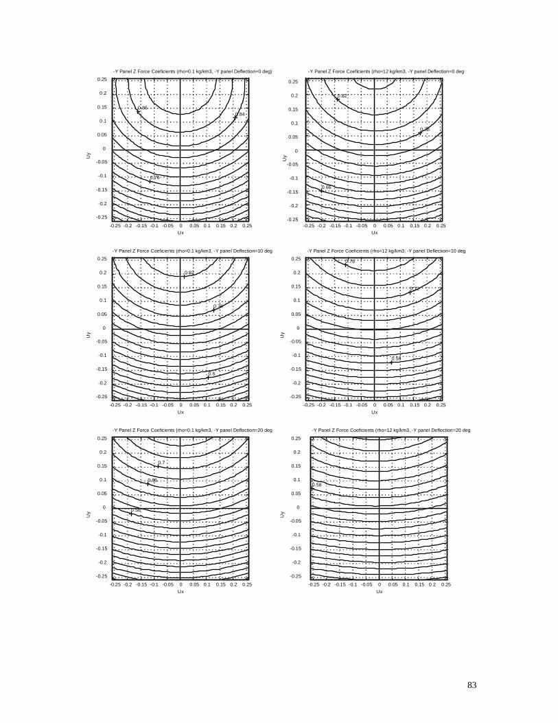
83

-0.25 -0.2 -0.15 -0.1 -0.05 0 0.05 0.1 0.15 0.2 0.25-0.25

-0.2

-0.15

-0.1

-0.05

0

0.05

0.1

0.15

0.2

0.25

0.66

0.78

0.82

-Y Panel Z Force Coeficients (rho=12 kg/km3, -Y panel Deflection=0 deg

Ux

Uy

-0.25 -0.2 -0.15 -0.1 -0.05 0 0.05 0.1 0.15 0.2 0.25

-0.25

-0.2

-0.15

-0.1

-0.05

0

0.05

0.1

0.15

0.2

0.25

0.58

0.72

0.76

-Y Panel Z Force Coeficients (rho=12 kg/km3, -Y panel Deflection=10 deg

Ux

Uy

-0.25 -0.2 -0.15 -0.1 -0.05 0 0.05 0.1 0.15 0.2 0.25

-0.25

-0.2

-0.15

-0.1

-0.05

0

0.05

0.1

0.15

0.2

0.25

0.58

-Y Panel Z Force Coeficients (rho=12 kg/km3, -Y panel Deflection=20 deg

Ux

Uy

-0.25 -0.2 -0.15 -0.1 -0.05 0 0.05 0.1 0.15 0.2 0.25

-0.25

-0.2

-0.15

-0.1

-0.05

0

0.05

0.1

0.15

0.2

0.25

0.76

0.840.86

-Y Panel Z Force Coeficients (rho=0.1 kg/km3, -Y panel Deflection=0 deg)

Ux

Uy

-0.25 -0.2 -0.15 -0.1 -0.05 0 0.05 0.1 0.15 0.2 0.25

-0.25

-0.2

-0.15

-0.1

-0.05

0

0.05

0.1

0.15

0.2

0.25

0.6

0.76

0.82

-Y Panel Z Force Coeficients (rho=0.1 kg/km3, -Y panel Deflection=10 deg

Ux

Uy

-0.25 -0.2 -0.15 -0.1 -0.05 0 0.05 0.1 0.15 0.2 0.25

-0.25

-0.2

-0.15

-0.1

-0.05

0

0.05

0.1

0.15

0.2

0.25

0.58

0.66

0.7

-Y Panel Z Force Coeficients (rho=0.1 kg/km3, -Y panel Deflection=20 deg

Ux

Uy

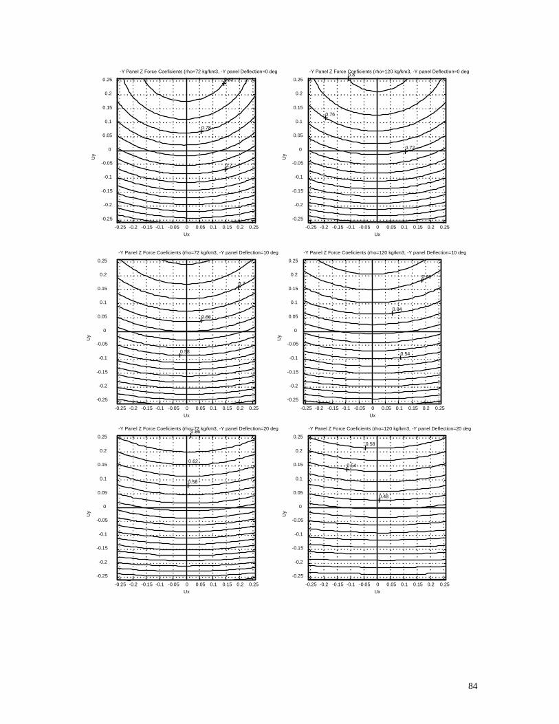
84

-0.25 -0.2 -0.15 -0.1 -0.05 0 0.05 0.1 0.15 0.2 0.25

-0.25

-0.2

-0.15

-0.1

-0.05

0

0.05

0.1

0.15

0.2

0.25

0.7

0.78

0.82

-Y Panel Z Force Coeficients (rho=72 kg/km3, -Y panel Deflection=0 deg

Ux

Uy

-0.25 -0.2 -0.15 -0.1 -0.05 0 0.05 0.1 0.15 0.2 0.25

-0.25

-0.2

-0.15

-0.1

-0.05

0

0.05

0.1

0.15

0.2

0.25

0.58

0.66

0.7

-Y Panel Z Force Coeficients (rho=72 kg/km3, -Y panel Deflection=10 deg

Ux

Uy

-0.25 -0.2 -0.15 -0.1 -0.05 0 0.05 0.1 0.15 0.2 0.25

-0.25

-0.2

-0.15

-0.1

-0.05

0

0.05

0.1

0.15

0.2

0.25

0.58

0.66-Y Panel Z Force Coeficients (rho=72 kg/km3, -Y panel Deflection=20 deg

Ux

Uy

0.62

-0.25 -0.2 -0.15 -0.1 -0.05 0 0.05 0.1 0.15 0.2 0.25

-0.25

-0.2

-0.15

-0.1

-0.05

0

0.05

0.1

0.15

0.2

0.25

0.72

0.76

0.8-Y Panel Z Force Coeficients (rho=120 kg/km3, -Y panel Deflection=0 deg

Ux

Uy

-0.25 -0.2 -0.15 -0.1 -0.05 0 0.05 0.1 0.15 0.2 0.25

-0.25

-0.2

-0.15

-0.1

-0.05

0

0.05

0.1

0.15

0.2

0.25

0.54

0.64

0.68

-Y Panel Z Force Coeficients (rho=120 kg/km3, -Y panel Deflection=10 deg

Ux

Uy

-0.25 -0.2 -0.15 -0.1 -0.05 0 0.05 0.1 0.15 0.2 0.25

-0.25

-0.2

-0.15

-0.1

-0.05

0

0.05

0.1

0.15

0.2

0.25

0.48

0.54

0.58

-Y Panel Z Force Coeficients (rho=120 kg/km3, -Y panel Deflection=20 deg

Ux

Uy

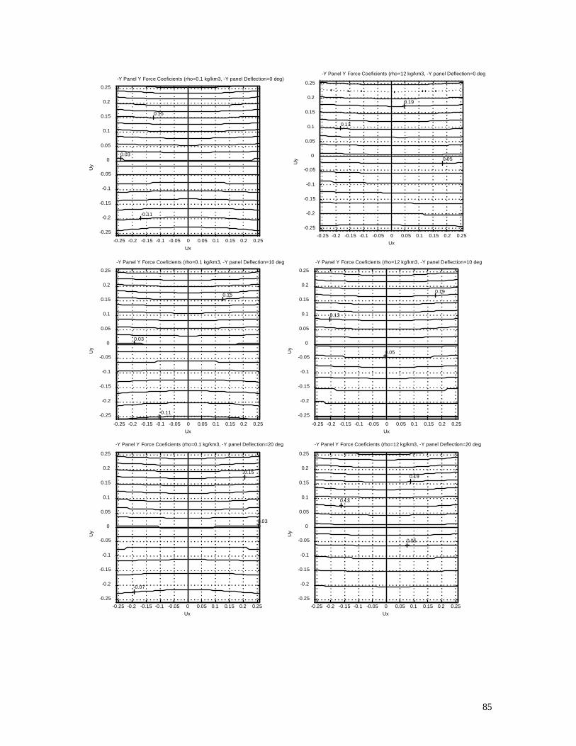
85

-0.25 -0.2 -0.15 -0.1 -0.05 0 0.05 0.1 0.15 0.2 0.25

-0.25

-0.2

-0.15

-0.1

-0.05

0

0.05

0.1

0.15

0.2

0.25

0.05

0.13

0.19

-Y Panel Y Force Coeficients (rho=12 kg/km3, -Y panel Deflection=0 deg

Ux

Uy

-0.25 -0.2 -0.15 -0.1 -0.05 0 0.05 0.1 0.15 0.2 0.25

-0.25

-0.2

-0.15

-0.1

-0.05

0

0.05

0.1

0.15

0.2

0.25

0.05

0.13

0.19

-Y Panel Y Force Coeficients (rho=12 kg/km3, -Y panel Deflection=10 deg

Ux

Uy

-0.25 -0.2 -0.15 -0.1 -0.05 0 0.05 0.1 0.15 0.2 0.25

-0.25

-0.2

-0.15

-0.1

-0.05

0

0.05

0.1

0.15

0.2

0.25

0.05

0.13

0.19

-Y Panel Y Force Coeficients (rho=12 kg/km3, -Y panel Deflection=20 deg

Ux

Uy

-0.25 -0.2 -0.15 -0.1 -0.05 0 0.05 0.1 0.15 0.2 0.25

-0.25

-0.2

-0.15

-0.1

-0.05

0

0.05

0.1

0.15

0.2

0.25

-0.11

0.03

0.15

-Y Panel Y Force Coeficients (rho=0.1 kg/km3, -Y panel Deflection=0 deg)

Ux

Uy

-0.25 -0.2 -0.15 -0.1 -0.05 0 0.05 0.1 0.15 0.2 0.25

-0.25

-0.2

-0.15

-0.1

-0.05

0

0.05

0.1

0.15

0.2

0.25

-0.11

0.03

0.15

-Y Panel Y Force Coeficients (rho=0.1 kg/km3, -Y panel Deflection=10 deg

Ux

Uy

-0.25 -0.2 -0.15 -0.1 -0.05 0 0.05 0.1 0.15 0.2 0.25

-0.25

-0.2

-0.15

-0.1

-0.05

0

0.05

0.1

0.15

0.2

0.25

-0.07

0.03

0.15

-Y Panel Y Force Coeficients (rho=0.1 kg/km3, -Y panel Deflection=20 deg

Ux

Uy

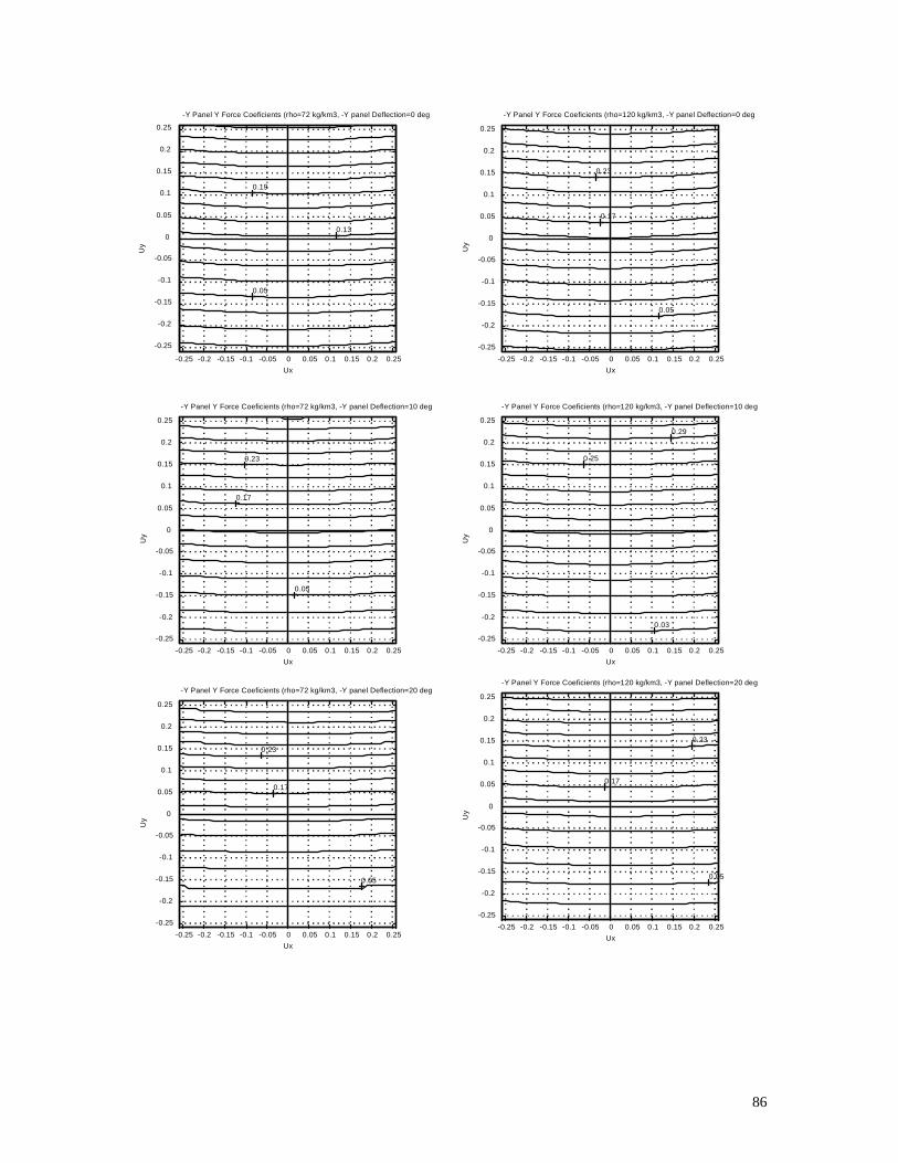
86

-0.25 -0.2 -0.15 -0.1 -0.05 0 0.05 0.1 0.15 0.2 0.25

-0.25

-0.2

-0.15

-0.1

-0.05

0

0.05

0.1

0.15

0.2

0.25

0.05

0.13

0.19

-Y Panel Y Force Coeficients (rho=72 kg/km3, -Y panel Deflection=0 deg

Ux

Uy

-0.25 -0.2 -0.15 -0.1 -0.05 0 0.05 0.1 0.15 0.2 0.25

-0.25

-0.2

-0.15

-0.1

-0.05

0

0.05

0.1

0.15

0.2

0.25

0.05

0.17

0.23

-Y Panel Y Force Coeficients (rho=72 kg/km3, -Y panel Deflection=10 deg

Ux

Uy

-0.25 -0.2 -0.15 -0.1 -0.05 0 0.05 0.1 0.15 0.2 0.25

-0.25

-0.2

-0.15

-0.1

-0.05

0

0.05

0.1

0.15

0.2

0.25

0.05

0.17

0.23

-Y Panel Y Force Coeficients (rho=72 kg/km3, -Y panel Deflection=20 deg

Ux

Uy

-0.25 -0.2 -0.15 -0.1 -0.05 0 0.05 0.1 0.15 0.2 0.25

-0.25

-0.2

-0.15

-0.1

-0.05

0

0.05

0.1

0.15

0.2

0.25

0.05

0.17

0.23

-Y Panel Y Force Coeficients (rho=120 kg/km3, -Y panel Deflection=0 deg

Ux

Uy

-0.25 -0.2 -0.15 -0.1 -0.05 0 0.05 0.1 0.15 0.2 0.25

-0.25

-0.2

-0.15

-0.1

-0.05

0

0.05

0.1

0.15

0.2

0.25

0.03

0.25

0.29

-Y Panel Y Force Coeficients (rho=120 kg/km3, -Y panel Deflection=10 deg

Ux

Uy

-0.25 -0.2 -0.15 -0.1 -0.05 0 0.05 0.1 0.15 0.2 0.25

-0.25

-0.2

-0.15

-0.1

-0.05

0

0.05

0.1

0.15

0.2

0.25

0.05

0.17

0.23

-Y Panel Y Force Coeficients (rho=120 kg/km3, -Y panel Deflection=20 deg

Ux

Uy

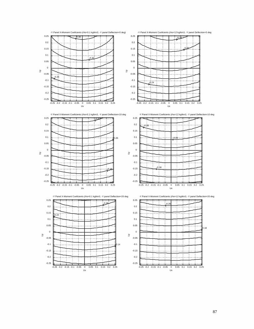
87

-0.25 -0.2 -0.15 -0.1 -0.05 0 0.05 0.1 0.15 0.2 0.25

-0.25

-0.2

-0.15

-0.1

-0.05

0

0.05

0.1

0.15

0.2

0.25

-0.24

-0.32

-0.34

-Y Panel X-Moment Coeficients (rho=12 kg/km3, -Y panel Deflection=0 deg

Ux

Uy

-0.25 -0.2 -0.15 -0.1 -0.05 0 0.05 0.1 0.15 0.2 0.25

-0.25

-0.2

-0.15

-0.1

-0.05

0

0.05

0.1

0.15

0.2

0.25

-0.18

-0.26

-0.28

-Y Panel X-Moment Coeficients (rho=12 kg/km3, -Y panel Deflection=10 deg

Ux

Uy

-0.25 -0.2 -0.15 -0.1 -0.05 0 0.05 0.1 0.15 0.2 0.25

-0.25

-0.2

-0.15

-0.1

-0.05

0

0.05

0.1

0.15

0.2

0.25

-0.18

-0.26

-Y Panel X-Moment Coeficients (rho=12 kg/km3, -Y panel Deflection=20 deg

Ux

Uy

-0.25 -0.2 -0.15 -0.1 -0.05 0 0.05 0.1 0.15 0.2 0.25

-0.25

-0.2

-0.15

-0.1

-0.05

0

0.05

0.1

0.15

0.2

0.25

-0.26

-0.32

-0.36

-Y Panel X-Moment Coeficients (rho=0.1 kg/km3, -Y panel Deflection=0 deg)

Ux

Uy

-0.25 -0.2 -0.15 -0.1 -0.05 0 0.05 0.1 0.15 0.2 0.25

-0.25

-0.2

-0.15

-0.1

-0.05

0

0.05

0.1

0.15

0.2

0.25

-0.18

-0.26

-0.32

-Y Panel X-Moment Coeficients (rho=0.1 kg/km3, -Y panel Deflection=10 deg

Ux

Uy

-0.25 -0.2 -0.15 -0.1 -0.05 0 0.05 0.1 0.15 0.2 0.25

-0.25

-0.2

-0.15

-0.1

-0.05

0

0.05

0.1

0.15

0.2

0.25

-0.14

-0.22

-0.26

-Y Panel X-Moment Coeficients (rho=0.1 kg/km3, -Y panel Deflection=20 deg

Ux

Uy

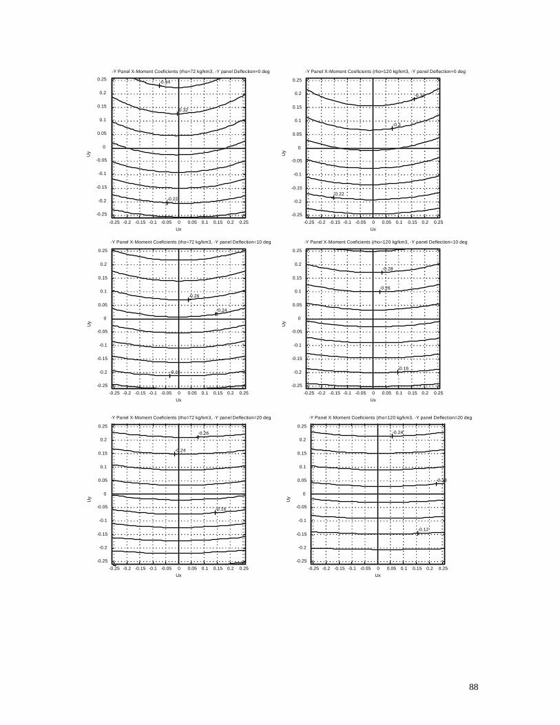
88

-0.25 -0.2 -0.15 -0.1 -0.05 0 0.05 0.1 0.15 0.2 0.25

-0.25

-0.2

-0.15

-0.1

-0.05

0

0.05

0.1

0.15

0.2

0.25

-0.22

-0.32

-0.34

-Y Panel X-Moment Coeficients (rho=72 kg/km3, -Y panel Deflection=0 deg

Ux

Uy

-0.25 -0.2 -0.15 -0.1 -0.05 0 0.05 0.1 0.15 0.2 0.25

-0.25

-0.2

-0.15

-0.1

-0.05

0

0.05

0.1

0.15

0.2

0.25

-0.16

-0.24

-0.26

-Y Panel X-Moment Coeficients (rho=72 kg/km3, -Y panel Deflection=10 deg

Ux

Uy

-0.25 -0.2 -0.15 -0.1 -0.05 0 0.05 0.1 0.15 0.2 0.25

-0.25

-0.2

-0.15

-0.1

-0.05

0

0.05

0.1

0.15

0.2

0.25

-0.16

-0.24

-0.26

-Y Panel X-Moment Coeficients (rho=72 kg/km3, -Y panel Deflection=20 deg

Ux

Uy

-0.25 -0.2 -0.15 -0.1 -0.05 0 0.05 0.1 0.15 0.2 0.25

-0.25

-0.2

-0.15

-0.1

-0.05

0

0.05

0.1

0.15

0.2

0.25

-0.22

-0.3

-0.32

-Y Panel X-Moment Coeficients (rho=120 kg/km3, -Y panel Deflection=0 deg

Ux

Uy

-0.25 -0.2 -0.15 -0.1 -0.05 0 0.05 0.1 0.15 0.2 0.25

-0.25

-0.2

-0.15

-0.1

-0.05

0

0.05

0.1

0.15

0.2

0.25

-0.16

-0.26

-0.28

-Y Panel X-Moment Coeficients (rho=120 kg/km3, -Y panel Deflection=10 deg

Ux

Uy

-0.25 -0.2 -0.15 -0.1 -0.05 0 0.05 0.1 0.15 0.2 0.25

-0.25

-0.2

-0.15

-0.1

-0.05

0

0.05

0.1

0.15

0.2

0.25

-0.12

-0.18

-0.24

-Y Panel X-Moment Coeficients (rho=120 kg/km3, -Y panel Deflection=20 deg

Ux

Uy

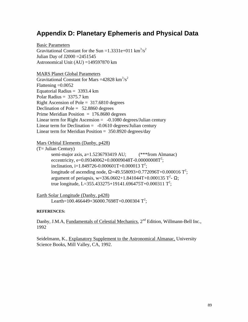
89

Appendix D: Planetary Ephemeris and Physical Data

Basic ParametersGravitational Constant for the Sun =1.3331e+011 km3/s2

Julian Day of J2000 =2451545Astronomical Unit (AU) =149597870 km

MARS Planet Global ParametersGravitational Constant for Mars =42828 km3/s2

Flattening =0.0052Equatorial Radius = 3393.4 kmPolar Radius = 3375.7 kmRight Ascension of Pole = 317.6810 degreesDeclination of Pole = 52.8860 degreesPrime Meridian Position = 176.8680 degreesLinear term for Right Ascension = -0.1080 degrees/Julian centuryLinear term for Declination = -0.0610 degrees/Julian centuryLinear term for Meridian Position = 350.8920 degrees/day

Mars Orbital Elements (Danby, p428)(T= Julian Century)

semi-major axis, a=1.5236793419 AU; (***from Almanac)eccentricity, e=0.09340062+0.00009048T-0.00000008T2;inclination, i=1.849726-0.000601T+0.000013 T2;longitude of ascending node, Ω=49.558093+0.772096T+0.000016 T2;argument of periapsis, w=336.0602+1.841044T+0.000135 T2- Ω;true longitude, L=355.433275+19141.696475T+0.000311 T2;

Earth Solar Longitude (Danby, p428)Learth=100.466449+36000.7698T+0.000304 T2;

REFERENCES:

Danby, J.M.A, Fundamentals of Celestial Mechanics, 2nd Edition, Willmann-Bell Inc.,1992

Seidelmann, K., Explanatory Supplement to the Astronomical Almanac, UniversityScience Books, Mill Valley, CA, 1992.

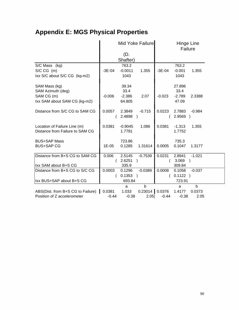
90

Appendix E: MGS Physical Properties

Mid Yoke Failure Hinge LineFailure

(D.Shafter)

S/C Mass (kg) 763.2 763.2S/C CG (m) -3E-04 -0.0011 1.355 -3E-04 -0.001 1.355Ixx S/C about S/C CG (kg-m2) 1043 1043

SAM Mass (kg) 39.34 27.896SAM Azimuth (deg) 33.4 33.4SAM CG (m) -0.006 -2.386 2.07 -0.023 -2.789 2.3388Ixx SAM about SAM CG (kg-m2) 64.805 47.09

Distance from S/C CG to SAM CG 0.0057 2.3849 -0.715 0.0223 2.7883 -0.984( 2.4898 ) ( 2.9569 )

Location of Failure Line (m) 0.0381 -0.9045 1.086 0.0381 -1.313 1.355Distance from Failure to SAM CG 1.7791 1.7752

BUS+SAP Mass 723.86 735.3BUS+SAP CG 1E-05 0.1285 1.31614 0.0005 0.1047 1.3177

Distance from B+S CG to SAM CG 0.006 2.5145 -0.7539 0.0231 2.8941 -1.021( 2.6251 ) ( 3.069 )

Ixx SAM about B+S CG 335.9 309.84Distance from B+S CG to S/C CG 0.0003 0.1296 -0.0389 0.0008 0.1058 -0.037

( 0.1353 ) ( 0.1122 )Ixx BUS+SAP about B+S CG 693.84 723.91

a b a bABS(Dist. from B+S CG to Failure) 0.0381 1.033 0.23014 0.0376 1.4177 0.0373Position of Z accelerometer -0.44 -0.38 2.05 -0.44 -0.38 2.05

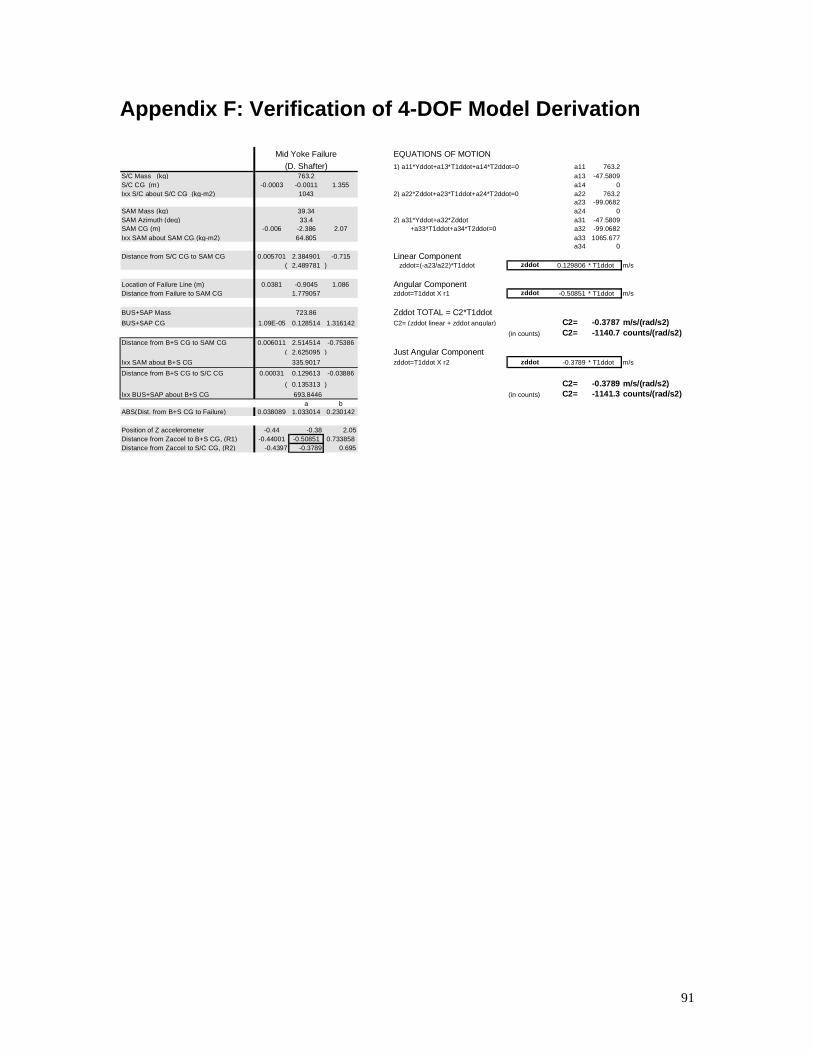
91

Appendix F: Verification of 4-DOF Model Derivation

Mid Yoke Failure EQUATIONS OF MOTION

(D. Shafter) 1) a11*Yddot+a13*T1ddot+a14*T2ddot=0 a11 763.2S/C Mass (kg) 763.2 a13 -47.5809S/C CG (m) -0.0003 -0.0011 1.355 a14 0Ixx S/C about S/C CG (kg-m2) 1043 2) a22*Zddot+a23*T1ddot+a24*T2ddot=0 a22 763.2

a23 -99.0682SAM Mass (kg) 39.34 a24 0SAM Azimuth (deg) 33.4 2) a31*Yddot+a32*Zddot a31 -47.5809SAM CG (m) -0.006 -2.386 2.07 +a33*T1ddot+a34*T2ddot=0 a32 -99.0682Ixx SAM about SAM CG (kg-m2) 64.805 a33 1065.677

a34 0

Distance from S/C CG to SAM CG 0.005701 2.384901 -0.715 Linear Component( 2.489781 ) zddot=(-a23/a22)*T1ddot zddot 0.129806 * T1ddot m/s

Location of Failure Line (m) 0.0381 -0.9045 1.086 Angular ComponentDistance from Failure to SAM CG 1.779057 zddot=T1ddot X r1 zddot -0.50851 * T1ddot m/s

BUS+SAP Mass 723.86 Zddot TOTAL = C2*T1ddotBUS+SAP CG 1.09E-05 0.128514 1.316142 C2= (zddot linear + zddot angular) C2= -0.3787 m/s/(rad/s2)

(in counts) C2= -1140.7 counts/(rad/s2)Distance from B+S CG to SAM CG 0.006011 2.514514 -0.75386

( 2.625095 ) Just Angular ComponentIxx SAM about B+S CG 335.9017 zddot=T1ddot X r2 zddot -0.3789 * T1ddot m/s

Distance from B+S CG to S/C CG 0.00031 0.129613 -0.03886

( 0.135313 ) C2= -0.3789 m/s/(rad/s2)Ixx BUS+SAP about B+S CG 693.8446 (in counts) C2= -1141.3 counts/(rad/s2)

a bABS(Dist. from B+S CG to Failure) 0.038089 1.033014 0.230142

Position of Z accelerometer -0.44 -0.38 2.05Distance from Zaccel to B+S CG, (R1) -0.44001 -0.50851 0.733858Distance from Zaccel to S/C CG, (R2) -0.4397 -0.3789 0.695

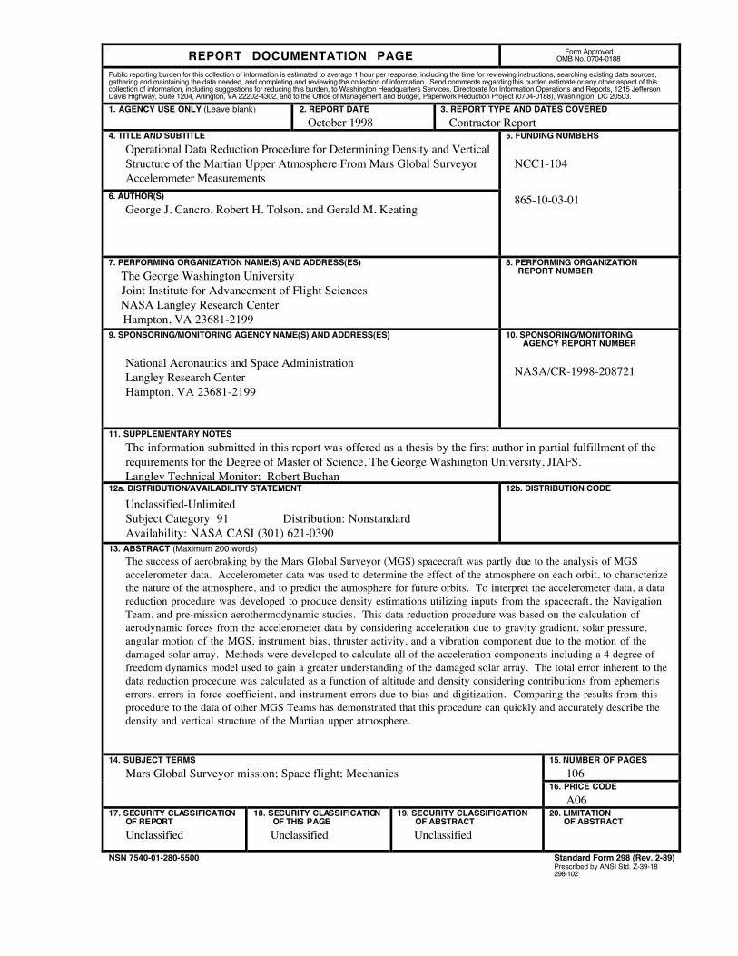
REPORT DOCUMENTATION PAGE Form ApprovedOMB No. 0704-0188

Public reporting burden for this collection of information is estimated to average 1 hour per response, including the time for reviewing instructions, searching existing data sources,gathering and maintaining the data needed, and completing and reviewing the collection of information. Send comments regarding this burden estimate or any other aspect of thiscollection of information, including suggestions for reducing this burden, to Washington Headquarters Services, Directorate for Information Operations and Reports, 1215 JeffersonDavis Highway, Suite 1204, Arlington, VA 22202-4302, and to the Office of Management and Budget, Paperwork Reduction Project (0704-0188), Washington, DC 20503.

1. AGENCY USE ONLY (Leave blank) 2. REPORT DATE

October 19983. REPORT TYPE AND DATES COVERED

Contractor Report4. TITLE AND SUBTITLE

Operational Data Reduction Procedure for Determining Density and VerticalStructure of the Martian Upper Atmosphere From Mars Global SurveyorAccelerometer Measurements

5. FUNDING NUMBERS

NCC1-104

6. AUTHOR(S)

George J. Cancro, Robert H. Tolson, and Gerald M. Keating865-10-03-01

7. PERFORMING ORGANIZATION NAME(S) AND ADDRESS(ES)

The George Washington University Joint Institute for Advancement of Flight Sciences NASA Langley Research Center Hampton, VA 23681-2199

8. PERFORMING ORGANIZATIONREPORT NUMBER

9. SPONSORING/MONITORING AGENCY NAME(S) AND ADDRESS(ES)

National Aeronautics and Space AdministrationLangley Research CenterHampton, VA 23681-2199

10. SPONSORING/MONITORINGAGENCY REPORT NUMBER

NASA/CR-1998-208721

11. SUPPLEMENTARY NOTES

The information submitted in this report was offered as a thesis by the first author in partial fulfillment of therequirements for the Degree of Master of Science, The George Washington University, JIAFS.Langley Technical Monitor: Robert Buchan

12a. DISTRIBUTION/AVAILABILITY STATEMENT

Unclassified-UnlimitedSubject Category 91 Distribution: NonstandardAvailability: NASA CASI (301) 621-0390

12b. DISTRIBUTION CODE

13. ABSTRACT (Maximum 200 words)

The success of aerobraking by the Mars Global Surveyor (MGS) spacecraft was partly due to the analysis of MGSaccelerometer data. Accelerometer data was used to determine the effect of the atmosphere on each orbit, to characterizethe nature of the atmosphere, and to predict the atmosphere for future orbits. To interpret the accelerometer data, a datareduction procedure was developed to produce density estimations utilizing inputs from the spacecraft, the NavigationTeam, and pre-mission aerothermodynamic studies. This data reduction procedure was based on the calculation ofaerodynamic forces from the accelerometer data by considering acceleration due to gravity gradient, solar pressure,angular motion of the MGS, instrument bias, thruster activity, and a vibration component due to the motion of thedamaged solar array. Methods were developed to calculate all of the acceleration components including a 4 degree offreedom dynamics model used to gain a greater understanding of the damaged solar array. The total error inherent to thedata reduction procedure was calculated as a function of altitude and density considering contributions from ephemeriserrors, errors in force coefficient, and instrument errors due to bias and digitization. Comparing the results from thisprocedure to the data of other MGS Teams has demonstrated that this procedure can quickly and accurately describe thedensity and vertical structure of the Martian upper atmosphere.

14. SUBJECT TERMS

Mars Global Surveyor mission; Space flight; Mechanics15. NUMBER OF PAGES

106

16. PRICE CODE

A0617. SECURITY CLASSIFICATION

OF REPORT

Unclassified

18. SECURITY CLASSIFICATIONOF THIS PAGE

Unclassified

19. SECURITY CLASSIFICATION OF ABSTRACT

Unclassified

20. LIMITATION OF ABSTRACT

NSN 7540-01-280-5500 Standard Form 298 (Rev. 2-89)Prescribed by ANSI Std. Z-39-18298-102