Operational Modal Analysis: Development of a structural ... · structural identification tool for accelerometric data of a flexible wing ... Patran/Nastran ... the first four mode

Institut Supérieur de l’Aéronautique et de l’Espace

Operational Modal Analysis: Development of a

structural identification tool for accelerometric

data of a flexible wing

Final Degree Project

February 2012

David Ramos López de Eguílaz (ISAE Supaero / University of the Basque Country)

Under supervision of Prof. Dr Joseph Morlier (ISAE/DMSM)

First of all I would like to thank my family, especially to

Laudelino, Felisa, Mireia and Nico for all their support during

this experience, as well as to Ana and my friends. In addition,

thanks to Joseph Morlier, for making this internship possible

and orienting my work, along with all the members of the

Structural Mechanics and Materials Department of SUPAERO,

which have always been willing to help me.

Index

1. Introduction ................................................................................................................................................. 1

2. Main objectives ............................................................................................................................................ 2

3. Theory .......................................................................................................................................................... 3

3.1. Modal Analysis .................................................................................................................................... 3

a. Experimental Modal Analysis (EMA) ........................................................................................... 4

b. Numerical Modal Analysis (NMA) ............................................................................................... 6

c. Operational Modal Analysis (OMA) ............................................................................................ 7

3.2. Operational Modal Analysis Methods ................................................................................................. 9

a. Combined Ambient System ........................................................................................................ 9

b. Other methods ........................................................................................................................... 10

3.3. Excitements ........................................................................................................................................ 11

4. Development .............................................................................................................................................. 15

4.1. Identify natural frequencies ............................................................................................................... 15

a. Continuous turbulence .............................................................................................................. 15

b. Discrete turbulence ................................................................................................................... 21

4.2. Change in natural frequencies due to damage and temperature changes ........................................ 23

a. Models ....................................................................................................................................... 23

b. Material ..................................................................................................................................... 25

c. Natural frequencies under temperature changes ..................................................................... 26

i. Plate ................................................................................................................................. 26

ii. Wing ................................................................................................................................. 27

d. Damage modeling in FEM .......................................................................................................... 28

i. Methods for modeling cracks .......................................................................................... 28

ii. Modeling damage in the plate ......................................................................................... 30

iii. Modeling damage in the wing ......................................................................................... 37

e. Natural frequencies shift due to damage .................................................................................. 38

i. Plate ................................................................................................................................. 38

ii. Wing ................................................................................................................................. 43

4.3. Combined influence of Temperature, damage location and damage length in natural

frequencies ......................................................................................................................................... 45

a. Plate ........................................................................................................................................... 45

b. Wing ........................................................................................................................................... 48

4.4. Transient Analyses under damage and temperature changes ........................................................... 50

4.5. Transient analyses under complex turbulence scenario .................................................................... 53

a. Excitement creation ................................................................................................................... 53

b. Responses .................................................................................................................................. 56

4.6. Transient Responses Database ........................................................................................................... 57

a. Analysis automation .................................................................................................................. 58

b. Analyses accomplishment .......................................................................................................... 61

5. Results and comments ................................................................................................................................ 63

6. References .................................................................................................................................................. 65

7. Annex 1: Databases table............................................................................................................................ 66

8. Annex 2: Software ....................................................................................................................................... 69

8.1. Patran/Nastran ................................................................................................................................... 69

8.2. Matlab ................................................................................................................................................ 70

8.3. Excel ................................................................................................................................................... 70

9. Annex 3: PCL code ...................................................................................................................................... 72

1

1. Introduction

Structural Health Monitoring (SHM) is a combination of words that has emerged around the late

1980s. However, it possibly dates back much earlier than that. Indeed, it may date back to the origins

of structural engineering.

Engineering structures are designed to be safe. The difficulty one trading in this regard is the desire

to construct something for a specific purpose out of a material of which one can never know enough

in terms of the material's properties as well as the environment the structure is going to operate in.

Regarding the latter, every gained knowledge about it is welcome; however, the needs are not

known at they must be covered by a safety factor which must be guessed. The less it is known about

the operational conditions of a structure and the performance of materials and structures, the higher

the safety factor will have to be. This is the risk and dilemma structural engineering is in.

Engineering structures are designed to withstand loads. These loads can be mechanical loads of a

static and/or dynamic nature. Loads can, however, also be of an environmental nature such as

temperature, humidity or chemical, and again the structure can be exposed to these loads in either a

static or even very short term and thus dynamic condition such as a thermo shock. Knowledge of

loads applied to a structure has to come from experience. This experience has been either gathered

on similar structures in the past or from assumptions. The safest way to design a structure is to

design it against an ultimate design limit load, which is the maximum load ever experienced with

such a structure added by a safety margin. Designing a structure against this load, however, makes

the structure heavy. Often, the maximum load of a structure may just occur once in the structure's

life, if ever at all. In that case one may start to question the extreme safety built in, specifically if the

maximum load applied would not result in any observable damage.

Loads applied to a structure are the reason for structural deterioration and hence resulting damage.

This damage may be generated at a microscopic level and may gradually progress until it becomes

observable and critical. Trading with this observability and criticality is the art of damage tolerant

design, which has allowed structures to become lighter weight. The way the damage accumulates is

of a fairly random nature; this requires careful means and procedure of inspection at well-defined

intervals.

The booming development of sensing technology in terms of sensors decreasing in size and cost, and

the combination with microprocessors with increasing power and enhanced materials design and

manufacturing in terms of functional materials or even electronic textiles have opened avenues in

merging structural design and maintenance with those advanced sensing, signal processing, and

materials manufacturing technologies. Taking advantage of this lateral integration is what SHM is

about. The central question in this field is therefore whether is possible to, without compromising

safety, make the structures better available, lighter, more cost efficient and more reliable by making

sensors (and maybe also actuators) to become an integral part of the structure. The answer could

somehow result in SHM, and a definition for SHM could possibly be the following.

SHM is the integration of sensing and possibly also actuation devices to allow the loading and

damaging conditions of a structure to be recorded, analyzed, localized, and predicted in a way that

nondestructive testing (NDT) becomes an integral part of the structure and material.

2

2. Main objectives

This work begins a series of projects researching about Structural Health Monitoring. This field tries

to identify the state of a structure while it is working, that is, when it is being excited by unknown

ambient excitations. As the first work in the field, this project aims to test the feasibility of different

approaches and to set the path for the following projects in the field.

On one hand, the first goal of the project is to build a finite elements model of the real structure, in

order to simulate damage (cracks) on it and run analyses under different situations of damage and

ambient conditions. The effect of both must be analyzed and compared and, in order to achieve such

an objective, the modal parameters of the structure will be used.

On the other hand, the second part of the project will consist of using the transient responses of the

structure under unknown excitations to monitor the health state of the structure. The approach to

pursue this objective is to create a platform which is able to simulate turbulence, in order to be used

as excitations for the simulated structure. Having the structure and the excitations, the transient

responses under different conditions of turbulence, damage and ambient conditions may be

obtained. Following a plan of experiments with the excitations, damage and ambient conditions as

variables allows creating a database of transient responses for different points of the structure, in

different directions, under different conditions of excitements, damage and ambient conditions. Such

a database would allow carrying out an output-only identification. This kind of identification has the

feature of being carried out without knowing the inputs that cause the outputs that are measured.

Due to that, the way to perform the identification is to measure real transient responses in the wing

by some accelerometers and the, compare this data with the database, so as to see which conditions

correspond to such a responses.

3

3. Theory

3.1. Modal Analysis: Modal analysis is a process that tries to analyze the dynamic response of a system. To do it, this

process defines the system by some properties, which are the natural frequencies, the mode shapes

and the damping ratio. As it is shown in the Figure 1, there are two main ways to do such an analysis,

which are the Experimental Modal Analysis (EMA) and the Numerical Modal Analysis (NMA). In a

design process both kind of analysis are usually complementary. Derived from the EMA, the

Operational Modal Analysis can also play an important role in the field of modal analysis.

Figure 1: Modal Analysis' Diagram

4

a. Experimental Modal Analysis:

Experimental Modal Analysis[1] is the oldest modal analysis, and it involves testing the system

experimentally. That means that the system is analyzed in a laboratory, where all the variables are

controlled. Therefore, in EMA both the inputs and the outputs are perfectly known. The main parts

of an EMA system are the excitation mechanisms, the transducers (accelerometers at the points to

be measured and load cells in the excitation point), an analog-digital converter and a PC to view the

data and analyze it. Apart from obtaining systems parameters, other applications of the experimental

analysis are listed below:

1. Predictive maintenance: In this case the objective is to detect possible failures in the

elements in order to substitute them before they fail. The vibration is measured to detect

increments in vibration, which could represent future problems.

2. Results checking: It is also useful to check whether the simplifications made in the

mathematical models are correct or not.

3. Vibrations control and isolation: The aim is to control how vibrations are transferred from

some elements to others.

4. Parameter obtaining: In this case it is used to determinate the mechanical parameters of the

system (mass, stiffness and damping, which is probably the most difficult to estimate).

5. Load recording: When it becomes important to know loads record.

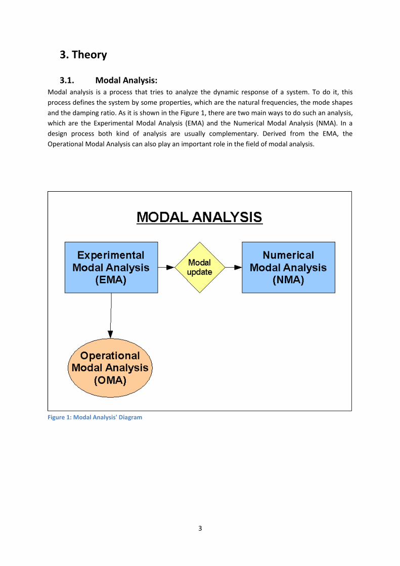
Regarding the system identification it is easy to observe that if the frequency of the excitement

varies, the output measured varies as well. If it is represented in an Response-Frequency diagram,

which is called Frequency Response Function (FRF), it is easy to see that at certain points the

amplitude grows considerably (Figure 2), whereas the input remains constant and only the frequency

in which is applied varies.

Figure 2: Frequency Response Function

If the data measured are referred to time instead of frequency, the FRF can be easily obtained using

a Fast Fourier Transform algorithm. Those points in which the amplitude grows (ω₁, ω₂ and ω₃)

represent the natural frequencies of the system, and the system must not be exited at those

frequencies during its life. Each of those points has a mode shape associated, which represents the

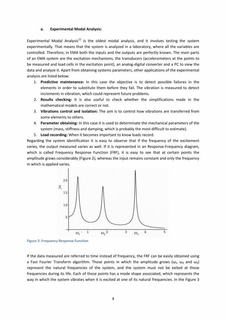
way in which the system vibrates when it is excited at one of its natural frequencies. In the Figure 3

5

the first four mode shapes of a cantilever beam are represented, showing first and second one in

detail.

Figure 3: Cantilever Vibration Modes

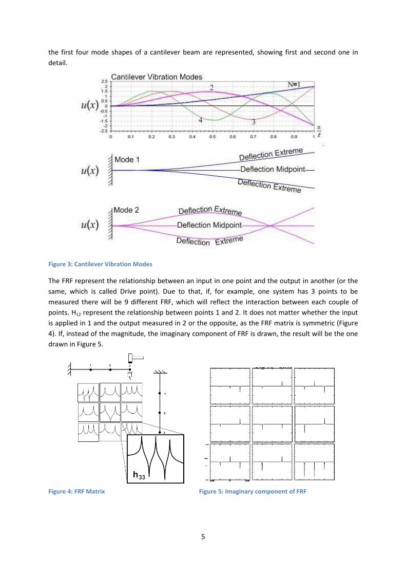
The FRF represent the relationship between an input in one point and the output in another (or the

same, which is called Drive point). Due to that, if, for example, one system has 3 points to be

measured there will be 9 different FRF, which will reflect the interaction between each couple of

points. H12 represent the relationship between points 1 and 2. It does not matter whether the input

is applied in 1 and the output measured in 2 or the opposite, as the FRF matrix is symmetric (Figure

4). If, instead of the magnitude, the imaginary component of FRF is drawn, the result will be the one

drawn in Figure 5.

Figure 4: FRF Matrix Figure 5: Imaginary component of FRF

6

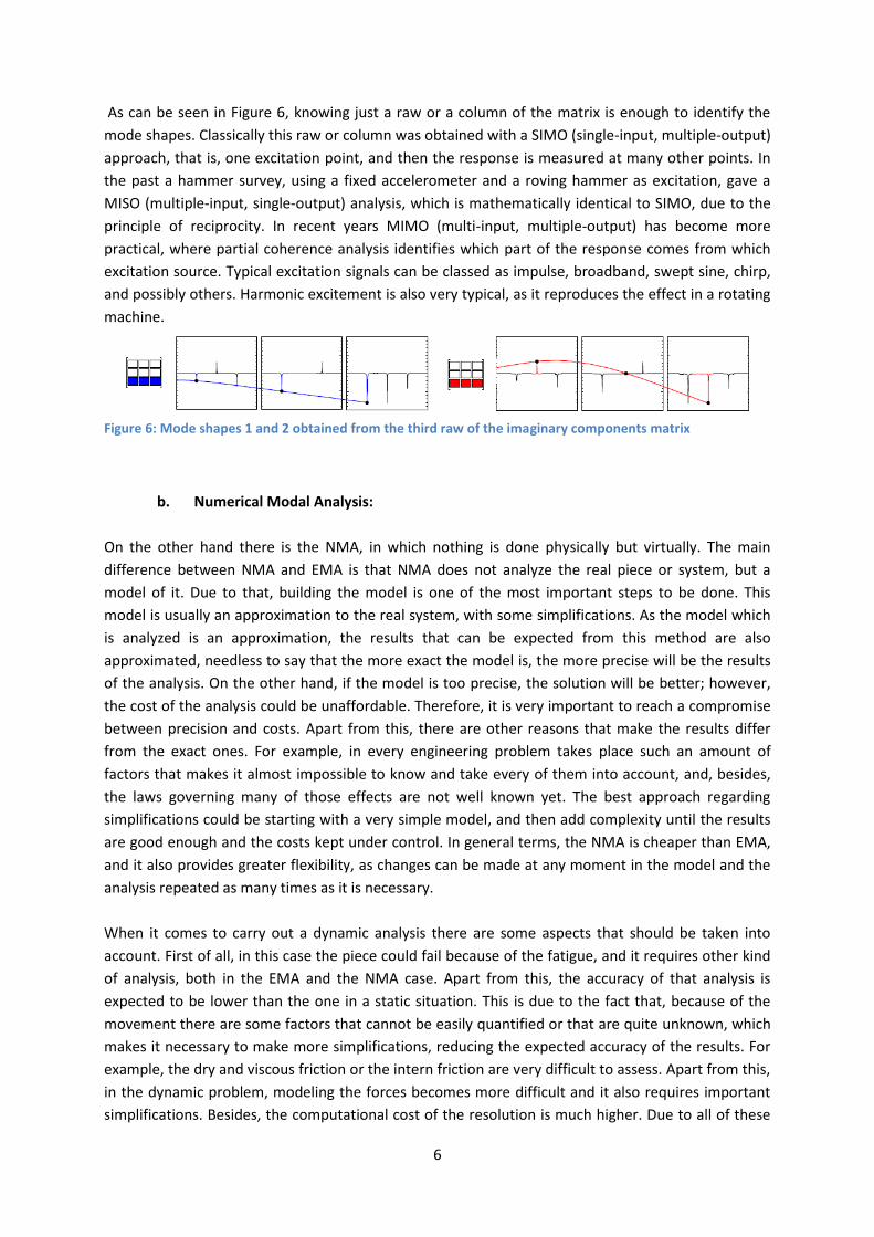
As can be seen in Figure 6, knowing just a raw or a column of the matrix is enough to identify the

mode shapes. Classically this raw or column was obtained with a SIMO (single-input, multiple-output)

approach, that is, one excitation point, and then the response is measured at many other points. In

the past a hammer survey, using a fixed accelerometer and a roving hammer as excitation, gave a

MISO (multiple-input, single-output) analysis, which is mathematically identical to SIMO, due to the

principle of reciprocity. In recent years MIMO (multi-input, multiple-output) has become more

practical, where partial coherence analysis identifies which part of the response comes from which

excitation source. Typical excitation signals can be classed as impulse, broadband, swept sine, chirp,

and possibly others. Harmonic excitement is also very typical, as it reproduces the effect in a rotating

machine.

Figure 6: Mode shapes 1 and 2 obtained from the third raw of the imaginary components matrix

b. Numerical Modal Analysis:

On the other hand there is the NMA, in which nothing is done physically but virtually. The main

difference between NMA and EMA is that NMA does not analyze the real piece or system, but a

model of it. Due to that, building the model is one of the most important steps to be done. This

model is usually an approximation to the real system, with some simplifications. As the model which

is analyzed is an approximation, the results that can be expected from this method are also

approximated, needless to say that the more exact the model is, the more precise will be the results

of the analysis. On the other hand, if the model is too precise, the solution will be better; however,

the cost of the analysis could be unaffordable. Therefore, it is very important to reach a compromise

between precision and costs. Apart from this, there are other reasons that make the results differ

from the exact ones. For example, in every engineering problem takes place such an amount of

factors that makes it almost impossible to know and take every of them into account, and, besides,

the laws governing many of those effects are not well known yet. The best approach regarding

simplifications could be starting with a very simple model, and then add complexity until the results

are good enough and the costs kept under control. In general terms, the NMA is cheaper than EMA,

and it also provides greater flexibility, as changes can be made at any moment in the model and the

analysis repeated as many times as it is necessary.

When it comes to carry out a dynamic analysis there are some aspects that should be taken into

account. First of all, in this case the piece could fail because of the fatigue, and it requires other kind

of analysis, both in the EMA and the NMA case. Apart from this, the accuracy of that analysis is

expected to be lower than the one in a static situation. This is due to the fact that, because of the

movement there are some factors that cannot be easily quantified or that are quite unknown, which

makes it necessary to make more simplifications, reducing the expected accuracy of the results. For

example, the dry and viscous friction or the intern friction are very difficult to assess. Apart from this,

in the dynamic problem, modeling the forces becomes more difficult and it also requires important

simplifications. Besides, the computational cost of the resolution is much higher. Due to all of these

7

simplifications the results obtained by a NMA in a dynamic analysis should be taken as approximated

and should be compared with the experimental analysis ones, in order to check the accuracy of the

NMA for that system. Here is where Modal Update comes. Modal Update consists of comparing the

experimental results with the numerical ones, in order to adjust the numerical parameters so as to

achieve a better accuracy in the numerical analyses.

c. Operational Modal Analysis:

The operational modal analysis is the newest of the three modal analysis techniques mentioned. The

main difference between this method and the previous ones is that it estimates the modal

parameters of a system when the input exciting the system is unknown.

This new approach it is necessary because there are many applications in which the operating

conditions vary greatly from the theoretical conditions employed in the modal test that could be

carried out in a laboratory, for example, in cars or aircrafts[1]. The fact that the conditions may be

different from those of the test may result in a lack of accuracy as far as vibration modes are

concerned. Due to that, it became necessary to develop a method which could analyze a system

while it is under operation conditions, which means that the input is unknown.

Other reason is that, traditionally, when it comes to analyze the state of a system (a bridge, a wing...)

this analysis was based on measures taken by people who led to subjective conclusions. OMA,

however, is a way to obtain objective measurements -with some restrictions-. Other clear example of

how important is to develop a method to analyze systems that are already working are the big

structures as bridges and buildings. Those kinds of structures are too complex to be modeled

accurately and exciting the real structure can be difficult and even dangerous. Apart from this, those

structures are always under ambient conditions, that are very difficult to measure and it is almost

impossible to completely suppress them during the test. As those excitations are unknown, an

output-only method is necessary to analyze them.

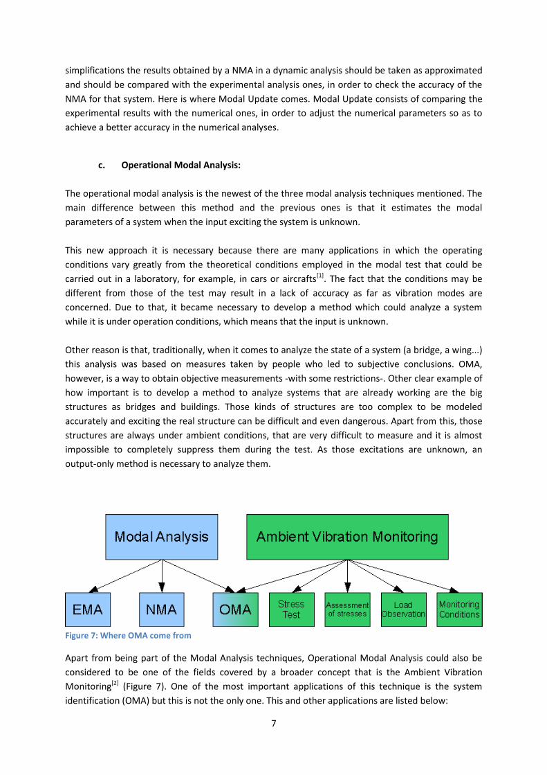
Figure 7: Where OMA come from

Apart from being part of the Modal Analysis techniques, Operational Modal Analysis could also be

considered to be one of the fields covered by a broader concept that is the Ambient Vibration

Monitoring[2] (Figure 7). One of the most important applications of this technique is the system

identification (OMA) but this is not the only one. This and other applications are listed below:

8

1. System identification: This application is the aforementioned OMA, which, instead of carrying

out stress tests to the systems and see whether the models fit the reality, consists of measuring

the ambient vibration. Those measures are recorded, evaluated and interpreted. Some examples

of the excitations that can be considered to be ambient could be micro-seismic phenomena,

wind, waves, etc. Apart from identifying the different parameters of the system, this method also

allows to estimate the remaining time service of the system, or to detect any damage on it. The

parameters that are often used to identify a system are the followings:

1.1. Eigenfrequencies and mode shapes: Eigenfrequencies describe the vibration behavior in the

linear static field. A mode shape belongs to every eigenfrequency. The actual oscillation of a

real structure is composed of the respective shares of the individual mode shapes.

1.2. Damping: Every system presents damping, and it is dependent on the frequencies,

representing an important feature in system identification. In fact it is an indicator of the

degree of exploitation of the structure, as the damping ratio rises considerably at the end of

the elastic field. In addition, dampings have an influence on the eigenfrequencies

themselves.

1.3. Deformations and displacements: Not only measuring deformations under defined loads but

also information of the structure deformations during measurement period.

1.4. Vibration intensity: It is a very good indicator for the stress of a structure by dynamic loads.

High intensities of a structure or individual members are very susceptible with regard to

fatigue-relevant damage mechanisms.

1.5. Trend cards: They represent a signal in the frequency-time domain by means of area

mapping. By coloring them the energy content of the vibration and therefore the respective

intensity can be determined, distinguishing the individual frequency peaks.

2. Stress test: Knowledge of the current stress condition of a structure and its individual load-

bearing elements is often particularly interesting. Examination is required, on the one hand, to

determine the existing current load-bearing safety level and to be able to introduce possibly

necessary immediate measures. On the other hand, it is an essential basis for the forecast of

future maintenance expenditures. An important assessment criterion to be mentioned in this

connection is the evaluation and interpretation of the vibration intensity of the respective

structure. This process can determine:

2.1. Static stresses

2.2. Dynamic stresses

2.3. Vibration elements

2.4. Stress of individual structural members.

3. Assessment of stresses: It must be carried out with regard to the actual condition and must

consider the predicted future development of the structural condition. The Ambient Vibration

Monitoring offers the possibility to carry out the assessment on the basis of objective

parameters. If these measuring results are combined with calculation models very good

predictions can be made by applying probabilistic approaches.

4. Load observation (Determination of external influences): The objective of the determination of

external influences (also called load observation) is the complete registering of traffic loads (in

the case of a bridge) or other influences acting on the structure. In this connection the induced

loads are not registered by means of a special balance but the dynamic reaction (response) of the

structure. This requires knowledge of the dynamic system behavior of the structure as acquired

by model calculations and/or experimentally (measurement).

9

5. Monitoring of the condition of structures: During health monitoring of structures global and

local structural properties are assessed on the basis of continuously recorded measured

variables. It is therefore possible to predict further development of the structural condition

sufficiently accurately. An additional aim is to provide simple and quick identification and

recording of changes in the load-bearing behavior.

3.2. Operational Modal Analysis Methods

a. Combined Ambient System

This measurement technique is similar to the “Operating Deflection Shapes” type procedure[19],

where one or more accelerometers are used as reference(s), and a series of roving accelerometers

are used for the responses at all the Degrees of Freedom (DOF’s), or all DOF’s are just measured

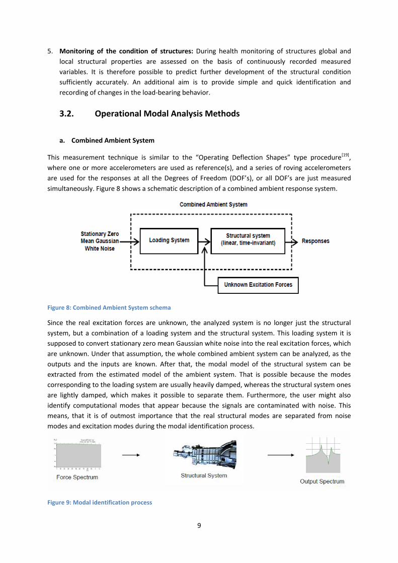
simultaneously. Figure 8 shows a schematic description of a combined ambient response system.

Figure 8: Combined Ambient System schema

Since the real excitation forces are unknown, the analyzed system is no longer just the structural

system, but a combination of a loading system and the structural system. This loading system it is

supposed to convert stationary zero mean Gaussian white noise into the real excitation forces, which

are unknown. Under that assumption, the whole combined ambient system can be analyzed, as the

outputs and the inputs are known. After that, the modal model of the structural system can be

extracted from the estimated model of the ambient system. That is possible because the modes

corresponding to the loading system are usually heavily damped, whereas the structural system ones

are lightly damped, which makes it possible to separate them. Furthermore, the user might also

identify computational modes that appear because the signals are contaminated with noise. This

means, that it is of outmost importance that the real structural modes are separated from noise

modes and excitation modes during the modal identification process.

Figure 9: Modal identification process

10

If the system is excited by white noise, the output spectrum contains full information of the structure

as all modes are excited equally. That happens because the power spectral density function Gxx of a

white noise excitation is constant (see Figure 9) and, taking into account that Gyy=|H(f)|²Gxx(f), all the

peaks in the output spectrum Gyy correspond to modes of the system. This is seldom the real case. In

general, the excitation has a spectral distribution, and the modes are weighted by it. Both the

“peaks” originating from the excitation signal and the structural modes are observed as “modes” in

the response. Apart from this, computational and measurement noise may as well appear as modes

in the output. Finally, the output spectra also present other non-physical modes, which are provoked

by harmonics in the system, very common in mechanical systems, as they are created by rotating

movements.

b. Other methods

Apart from this approach, there are many other methods developed in order to carry out Modal

Analysis[19]; however, the aim of this project is to research about other approaches of identifying the

state of a structure. Due to that, none of those methods will be used, and explaining them in detail is

beyond the scope of the project. For this reason the most important of them will be just presented in

the following schema:

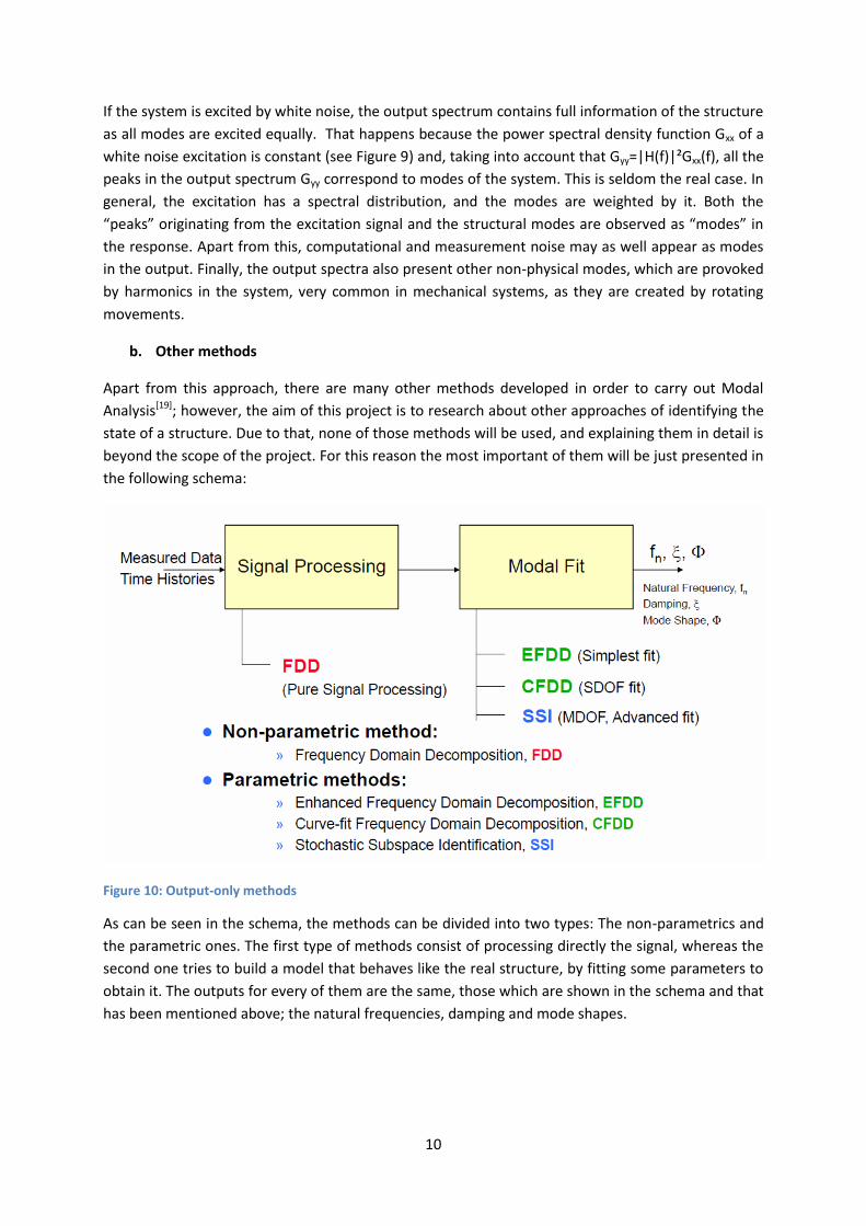
Figure 10: Output-only methods

As can be seen in the schema, the methods can be divided into two types: The non-parametrics and

the parametric ones. The first type of methods consist of processing directly the signal, whereas the

second one tries to build a model that behaves like the real structure, by fitting some parameters to

obtain it. The outputs for every of them are the same, those which are shown in the schema and that

has been mentioned above; the natural frequencies, damping and mode shapes.

11

3.3. Excitements

When it comes to represent the real behavior of a structural system, it is very important to build a

good model of the system, and, for carrying out certain kind of analyses, an input is needed,

therefore making necessary to define the signals to apply. In the field of Ambient Monitoring, some

excitations are very common, whereas other ones are more specific for certain kinds of structures.

One of the potential fields of the ambient vibration monitoring techniques is to check the health

state of bridges. For this case, for example, the excitations considered are different for those

considered when analyzing an aircraft or a building. First of all, noise must be considered. Not the

noise coming from cars, for example, but noise in the signal. It creates random fluctuations of small

amplitude in the signal. This effect can come from different sources which are not well known and do

not affect greatly to the system, for example, the constant breaking of the water against the bridge.

Other example could be the wind. When the wind changes its direction or its magnitude, the

incidence surface changes and obviously the generated forces change, however, when the wind

remains constant in direction and magnitude, the generated force is not exactly steady, and it

fluctuates randomly from the theoretical state. This is only one example of how the noise can be

generated. In a general case, the noise will be assumed to be of constant magnitude in every

frequency, what is called “white noise”. Apart from being a realistic assumption, considering noise as

white noise has the advantage of getting a constant spectrum in the input. It means that, being the

spectrum of the response the product of the input by the system features, every peak or shape found

in the response will correspond to the system, allowing making identification. This kind of excitation

becomes important when the sensors are good enough, as less accurate sensors are not able to

reproduce this kind of signal in a good way. In the case of a plane the white noise represents the part

of the flight in which continuous turbulence -no abnormal situation- takes place. Strong turbulence

cases or bird strikes will be represented by other kind of excitements, leaving white noise just for the

normal flight.

Other important type of excitation in the bridges is the one generated by people walking or cars

crossing the bridge. This kind of forces can be modeled quite well as harmonic excitations of different

frequencies. For pedestrians, this frequency tends to be lower than 4Hz.

In the case of an aircraft, the forces that have to be modeled for an analysis are slightly different. It is

a well-known but unfortunate feature of air travel that aircraft regularly encounter atmospheric

turbulence (or ‘rough air’) of varying degrees of severity. Turbulence may be considered as

movement of the air through which the aircraft passes. Any component of the velocity of the air (so-

called ‘gust velocity’) that is normal to the flight path will change the effective incidence of the

aerodynamic surfaces, so causing sudden changes in the lift forces and hence a dynamic response of

the aircraft involving flexible deformation; gust inputs are also considered along the flight path. The

response will involve both the rigid body and flexible modes.

Turbulence, although a complicated phenomenon, is normally considered for design purposes in one

of two idealized categories[12], namely:

(a) discrete gusts, where the gust velocity varies in a deterministic manner, often in the form of

a ‘1- cosine’ shape (i.e. there is an idealized discrete ‘event’ that the aircraft encounters), and

(b) continuous turbulence, where the gust velocity is assumed to vary in a random manner.

12

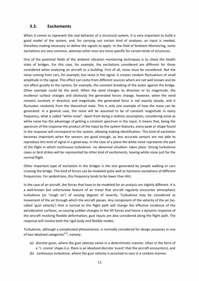
The difference between the two types of turbulence may be seen in Figure 11. The discrete gust

response is solved in the time domain whereas the continuous turbulence response is usually

determined in the frequency domain via a power spectral density method. Gusts and turbulence may

be vertical, lateral or at any orientation to the flight path, but vertical and lateral cases are normally

treated separately. Thus, for a symmetric aircraft, a vertical gust will give rise to heave (or

plunge)/pitch motions whereas a lateral gust will cause sideslip/yaw/roll motions; all these motions

will be coupled for an asymmetric aircraft.

Figure 11: Discrete and continuous Gusts represented

The continuous Gust is very easy to be modeled, because, as has been said before, it can be

represented as white noise. However, discrete gusts are not so easy to model and some simplified

models can help to do so:

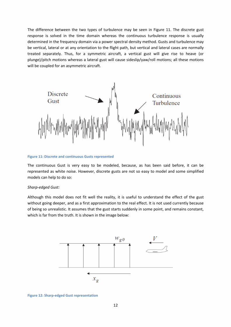
Sharp-edged Gust:

Although this model does not fit well the reality, it is useful to understand the effect of the gust

without going deeper, and as a first approximation to the real effect. It is not used currently because

of being so unrealistic. It assumes that the gust starts suddenly in some point, and remains constant,

which is far from the truth. It is shown in the image below:

Figure 12: Sharp-edged Gust representation

13

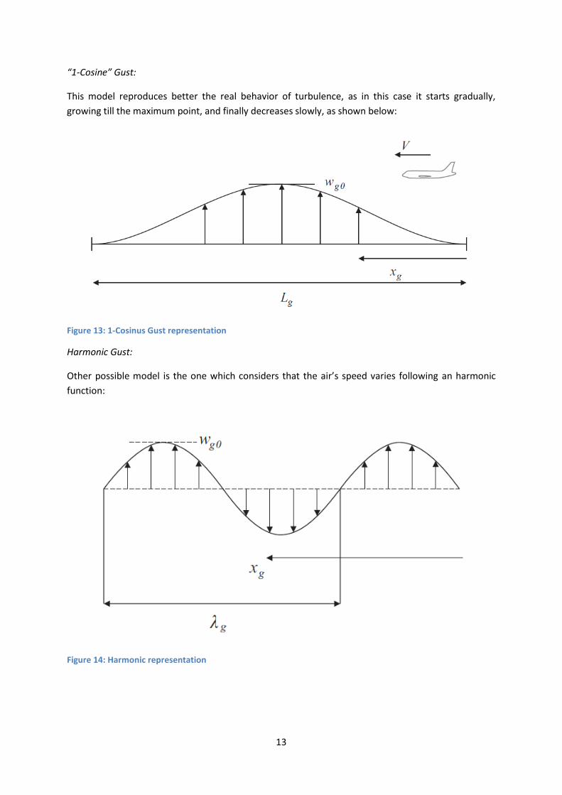
“1-Cosine” Gust:

This model reproduces better the real behavior of turbulence, as in this case it starts gradually,

growing till the maximum point, and finally decreases slowly, as shown below:

Figure 13: 1-Cosinus Gust representation

Harmonic Gust:

Other possible model is the one which considers that the air’s speed varies following an harmonic

function:

Figure 14: Harmonic representation

14

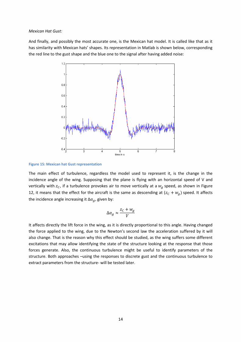
Mexican Hat Gust:

And finally, and possibly the most accurate one, is the Mexican hat model. It is called like that as it

has similarity with Mexican hats’ shapes. Its representation in Matlab is shown below, corresponding

the red line to the gust shape and the blue one to the signal after having added noise:

Figure 15: Mexican hat Gust representation

The main effect of turbulence, regardless the model used to represent it, is the change in the

incidence angle of the wing. Supposing that the plane is flying with an horizontal speed of V and

vertically with , if a turbulence provokes air to move vertically at a speed, as shown in Figure

12, it means that the effect for the aircraft is the same as descending at ( speed. It affects

the incidence angle increasing it Δ , given by:

It affects directly the lift force in the wing, as it is directly proportional to this angle. Having changed

the force applied to the wing, due to the Newton’s second law the acceleration suffered by it will

also change. That is the reason why this effect should be studied, as the wing suffers some different

excitations that may allow identifying the state of the structure looking at the response that those

forces generate. Also, the continuous turbulence might be useful to identify parameters of the

structure. Both approaches –using the responses to discrete gust and the continuous turbulence to

extract parameters from the structure- will be tested later.

15

4. Development

4.1. Identify natural frequencies

As has been introduced in the theory, there are two different kinds of gusts: The discrete gust and

the continuous one. In this chapter the usefulness of both in identifying modal parameters will be

tested. The model used for those cases will be the simplest one, which is a cantilever plate, having

more or less the size of a wing, but with a thickness of few millimeters. That is because the aim of

this part is not to obtain accurate results, but only to check whether those situations of continuous

and discrete turbulences are useful or not to determine modal parameters. The parameters that will

be obtained will be the natural frequencies, as they allow identifying damage or temperature

changes in the structure.

a. Under continuous turbulence

When a plane is flying, it is not always under discrete turbulences or birds strikes. This part of the

flight could be called continuous turbulence or ambient conditions. Although discrete turbulences or

bird strikes are very useful to obtain a rich transient response and carry out an Operational Modal

Analysis, the vibrations measured just under ambient conditions could also be useful to identify some

modal parameters. Guessing that those ambient excitations have the shape of white noise -which is

just a hypothesis- it becomes easy to identify the natural frequencies excited, as the peaks in the

frequency content of the spectrum will correspond to them, being flat the spectrum of a white noise

signal.

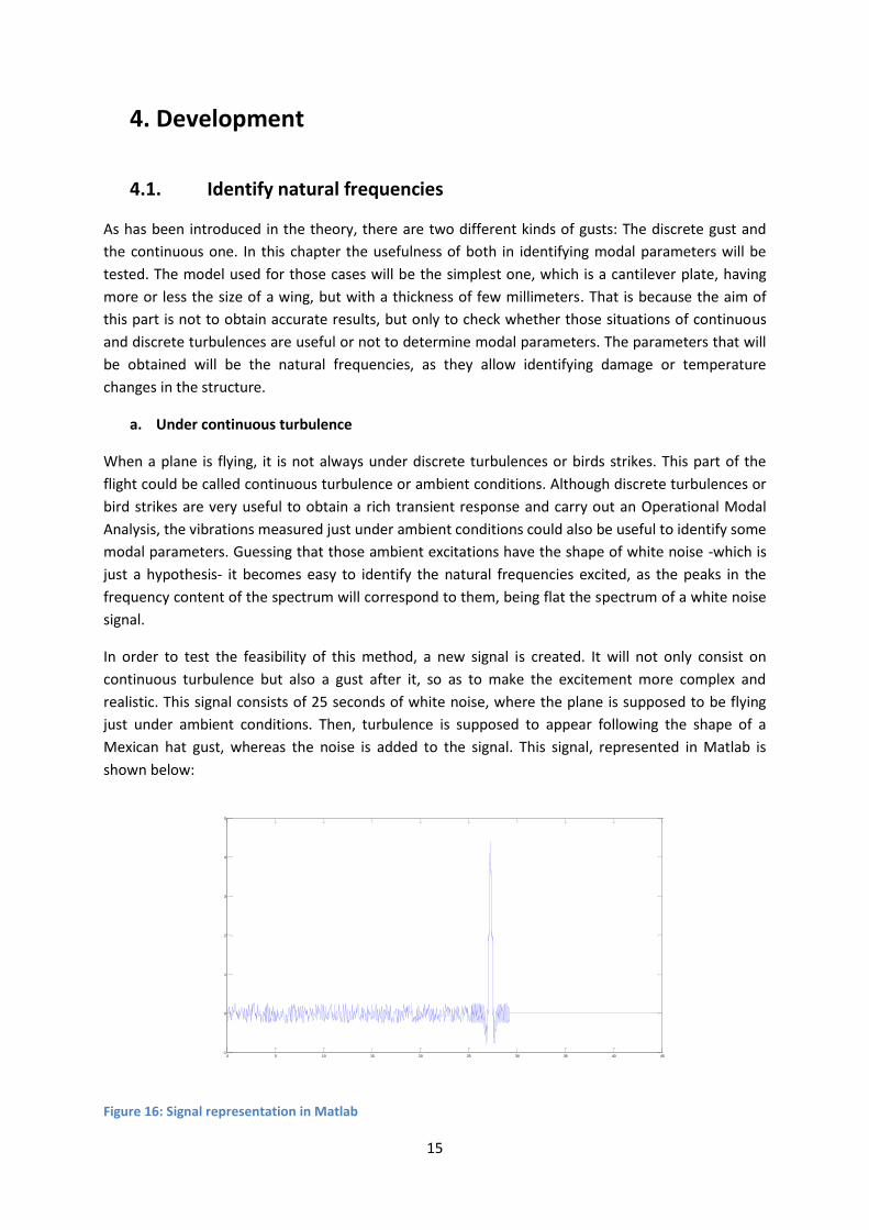
In order to test the feasibility of this method, a new signal is created. It will not only consist on

continuous turbulence but also a gust after it, so as to make the excitement more complex and

realistic. This signal consists of 25 seconds of white noise, where the plane is supposed to be flying

just under ambient conditions. Then, turbulence is supposed to appear following the shape of a

Mexican hat gust, whereas the noise is added to the signal. This signal, represented in Matlab is

shown below:

Figure 16: Signal representation in Matlab

0 5 10 15 20 25 30 35 40 45-1

0

1

2

3

4

5

16

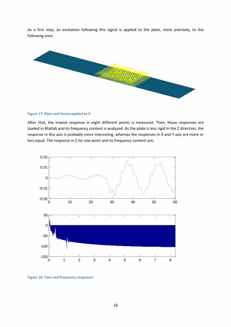
As a first step, an excitation following this signal is applied to the plate, more precisely, to the

following area:

Figure 17: Plate and forces applied to it

After that, the triaxial response in eight different points is measured. Then, those responses are

loaded in Matlab and its frequency content is analyzed. As the plate is less rigid in the Z direction, the

response in this axis is probably more interesting, whereas the responses in X and Y axis are more or

less equal. The response in Z for one point and its frequency content are:

Figure 18: Time and frequency responses

0 10 20 30 40 50 60-0.02

-0.01

0

0.01

0.02

0 1 2 3 4 5 6 7 8-150

-100

-50

0

50

17

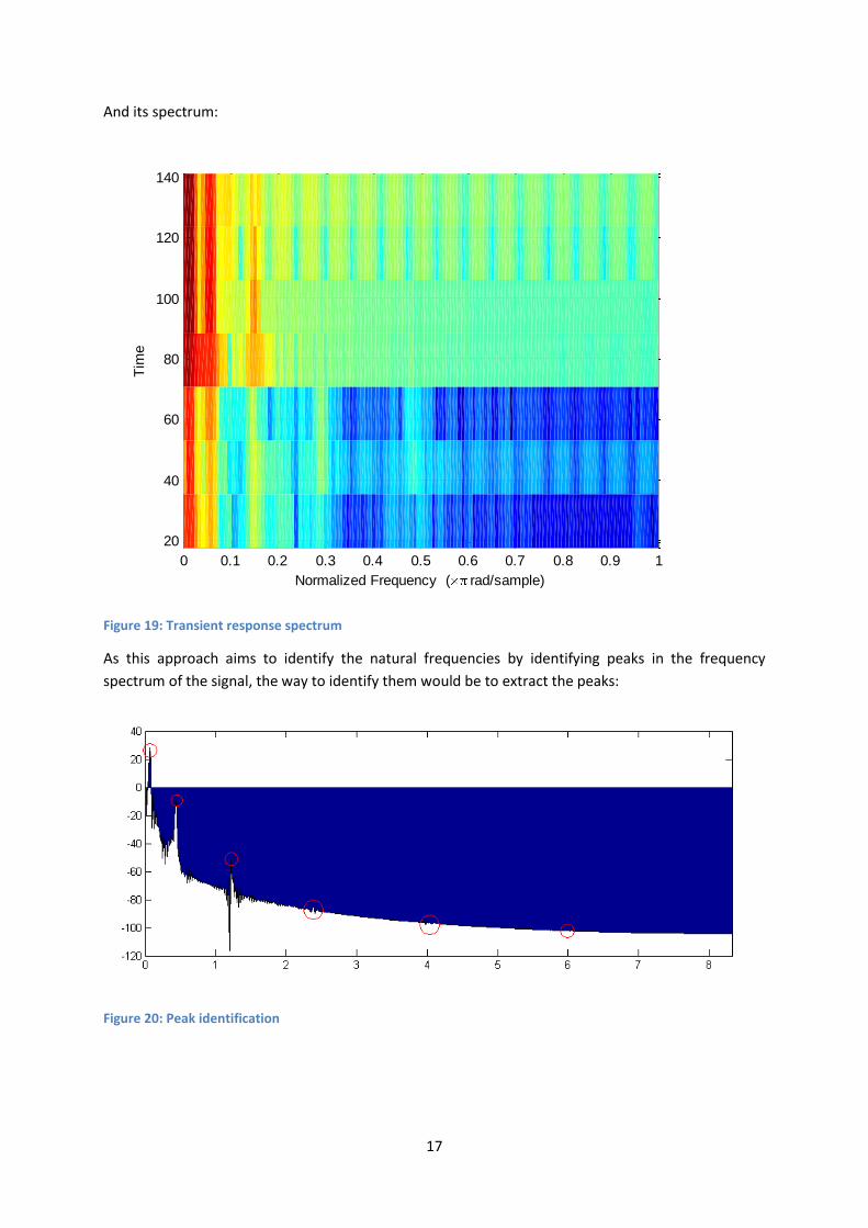
And its spectrum:

Figure 19: Transient response spectrum

As this approach aims to identify the natural frequencies by identifying peaks in the frequency

spectrum of the signal, the way to identify them would be to extract the peaks:

Figure 20: Peak identification

0 0.1 0.2 0.3 0.4 0.5 0.6 0.7 0.8 0.9 1

20

40

60

80

100

120

140

Normalized Frequency ( rad/sample)

Tim

e

18

At first sight, the three first peaks are obvious, and they are located approximately in 0.1, 0.4 and 2.4

Hz. By zooming on the image, it can be seen that the first peak is around 0.07, the second one around

0.44 and the third one at 1.23. The fourth peak is not as clear as the previous ones, however, it is still

easy to be identified, as a clear perturbation can be seen in the line. It is located at 2.4 Hz

approximately. Besides, the same behavior can be observed around 4 Hz. Finally, although is it more

difficult to be appreciated, there is also a little change in the behavior around 6 Hz. This case is

clearer when zooming the plot; however, there is no clear peak to identify, but a series of points that

are not exactly in the line.

In order to test whether the approach of identifying natural frequencies by checking the response

generated by ambient excitations works or not, the model has been analyzed also in Nastran, to

obtain the natural frequencies. The frequencies obtained are:

Mode Frequency

1 7.01E-02

2 4.39E-01

3 8.24E-01

4 1.23E+00

5 2.42E+00

6 2.51E+00

7 4.01E+00

8 4.29E+00

9 6.01E+00

10 6.23E+00

Table 1: Natural frequencies

Those results confirm that the followed approach has been correct, as the frequencies which were

obtained by identifying peaks correspond to the real ones. The first peak corresponds to the first

natural frequency, the second one to the second mode, the third to the fourth mode, the fourth to

the fifth mode, the fifth to the seventh mode and the sixth to the ninth one. It leads to the

conclusion that the modes which are represented by peaks are very easily identifiable and accurate;

however, not all the modes are represented by peaks. That is because, due to the area and the

direction in which the force has been applied, only the bending modes have been excited. By

representing the shape of each mode, every natural frequency can be associated to either a bending

mode or a torsional one:

19

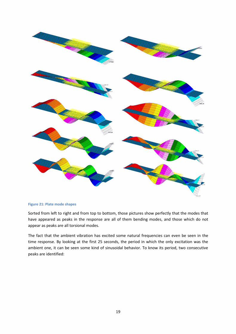
Figure 21: Plate mode shapes

Sorted from left to right and from top to bottom, those pictures show perfectly that the modes that

have appeared as peaks in the response are all of them bending modes, and those which do not

appear as peaks are all torsional modes.

The fact that the ambient vibration has excited some natural frequencies can even be seen in the

time response. By looking at the first 25 seconds, the period in which the only excitation was the

ambient one, it can be seen some kind of sinusoidal behavior. To know its period, two consecutive

peaks are identified:

20

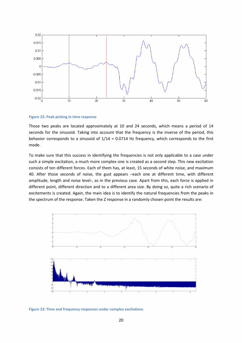
Figure 22: Peak picking in time response

Those two peaks are located approximately at 10 and 24 seconds, which means a period of 14

seconds for the sinusoid. Taking into account that the frequency is the inverse of the period, this

behavior corresponds to a sinusoid of 1/14 = 0.0714 Hz frequency, which corresponds to the first

mode.

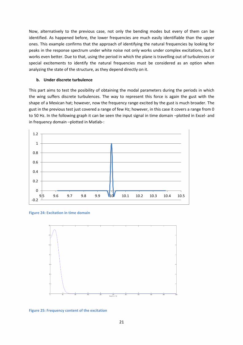
To make sure that this success in identifying the frequencies is not only applicable to a case under

such a simple excitation, a much more complex one is created as a second step. This new excitation

consists of ten different forces. Each of them has, at least, 15 seconds of white noise, and maximum

40. After those seconds of noise, the gust appears –each one at different time, with different

amplitude, length and noise level-, as in the previous case. Apart from this, each force is applied in

different point, different direction and to a different area size. By doing so, quite a rich scenario of

excitements is created. Again, the main idea is to identify the natural frequencies from the peaks in

the spectrum of the response. Taken the Z response in a randomly chosen point the results are:

Figure 23: Time and frequency responses under complex excitations

0 10 20 30 40 50 60-3

-2

-1

0

1

2

3

4

0 1 2 3 4 5 6 7 8-60

-40

-20

0

20

40

60

80

100

120

140

21

Now, alternatively to the previous case, not only the bending modes but every of them can be

identified. As happened before, the lower frequencies are much easily identifiable than the upper

ones. This example confirms that the approach of identifying the natural frequencies by looking for

peaks in the response spectrum under white noise not only works under complex excitations, but it

works even better. Due to that, using the period in which the plane is travelling out of turbulences or

special excitements to identify the natural frequencies must be considered as an option when

analyzing the state of the structure, as they depend directly on it.

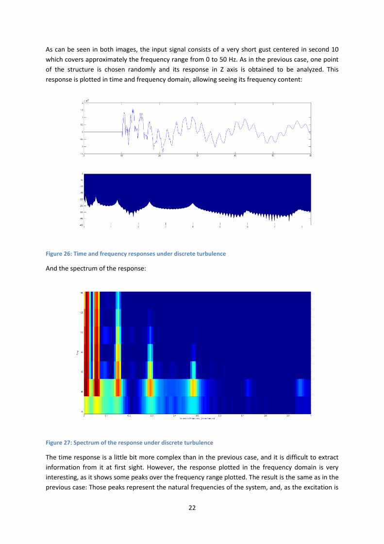
b. Under discrete turbulence

This part aims to test the posibility of obtaining the modal parameters during the periods in which

the wing suffers discrete turbulences. The way to represent this force is again the gust with the

shape of a Mexican hat; however, now the frequency range excited by the gust is much broader. The

gust in the previous test just covered a range of few Hz; however, in this case it covers a range from 0

to 50 Hz. In the following graph it can be seen the input signal in time domain –plotted in Excel- and

in frequency domain –plotted in Matlab-:

Figure 24: Excitation in time domain

Figure 25: Frequency content of the excitation

-0.2

0

0.2

0.4

0.6

0.8

1

1.2

9.5 9.6 9.7 9.8 9.9 10 10.1 10.2 10.3 10.4 10.5

22

As can be seen in both images, the input signal consists of a very short gust centered in second 10

which covers approximately the frequency range from 0 to 50 Hz. As in the previous case, one point

of the structure is chosen randomly and its response in Z axis is obtained to be analyzed. This

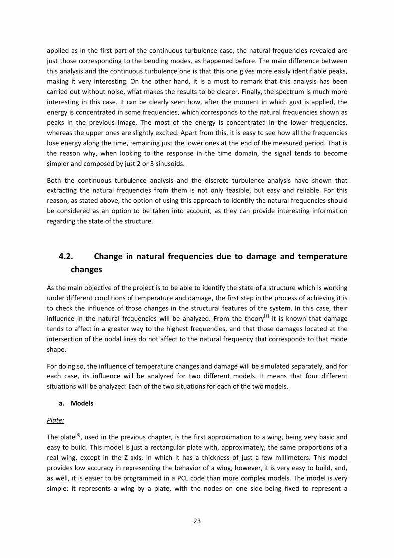
response is plotted in time and frequency domain, allowing seeing its frequency content:

Figure 26: Time and frequency responses under discrete turbulence

And the spectrum of the response:

Figure 27: Spectrum of the response under discrete turbulence

The time response is a little bit more complex than in the previous case, and it is difficult to extract

information from it at first sight. However, the response plotted in the frequency domain is very

interesting, as it shows some peaks over the frequency range plotted. The result is the same as in the

previous case: Those peaks represent the natural frequencies of the system, and, as the excitation is

23

applied as in the first part of the continuous turbulence case, the natural frequencies revealed are

just those corresponding to the bending modes, as happened before. The main difference between

this analysis and the continuous turbulence one is that this one gives more easily identifiable peaks,

making it very interesting. On the other hand, it is a must to remark that this analysis has been

carried out without noise, what makes the results to be clearer. Finally, the spectrum is much more

interesting in this case. It can be clearly seen how, after the moment in which gust is applied, the

energy is concentrated in some frequencies, which corresponds to the natural frequencies shown as

peaks in the previous image. The most of the energy is concentrated in the lower frequencies,

whereas the upper ones are slightly excited. Apart from this, it is easy to see how all the frequencies

lose energy along the time, remaining just the lower ones at the end of the measured period. That is

the reason why, when looking to the response in the time domain, the signal tends to become

simpler and composed by just 2 or 3 sinusoids.

Both the continuous turbulence analysis and the discrete turbulence analysis have shown that

extracting the natural frequencies from them is not only feasible, but easy and reliable. For this

reason, as stated above, the option of using this approach to identify the natural frequencies should

be considered as an option to be taken into account, as they can provide interesting information

regarding the state of the structure.

4.2. Change in natural frequencies due to damage and temperature

changes

As the main objective of the project is to be able to identify the state of a structure which is working

under different conditions of temperature and damage, the first step in the process of achieving it is

to check the influence of those changes in the structural features of the system. In this case, their

influence in the natural frequencies will be analyzed. From the theory[1] it is known that damage

tends to affect in a greater way to the highest frequencies, and that those damages located at the

intersection of the nodal lines do not affect to the natural frequency that corresponds to that mode

shape.

For doing so, the influence of temperature changes and damage will be simulated separately, and for

each case, its influence will be analyzed for two different models. It means that four different

situations will be analyzed: Each of the two situations for each of the two models.

a. Models

Plate:

The plate[3], used in the previous chapter, is the first approximation to a wing, being very basic and

easy to build. This model is just a rectangular plate with, approximately, the same proportions of a

real wing, except in the Z axis, in which it has a thickness of just a few millimeters. This model

provides low accuracy in representing the behavior of a wing, however, it is very easy to build, and,

as well, it is easier to be programmed in a PCL code than more complex models. The model is very

simple: it represents a wing by a plate, with the nodes on one side being fixed to represent a

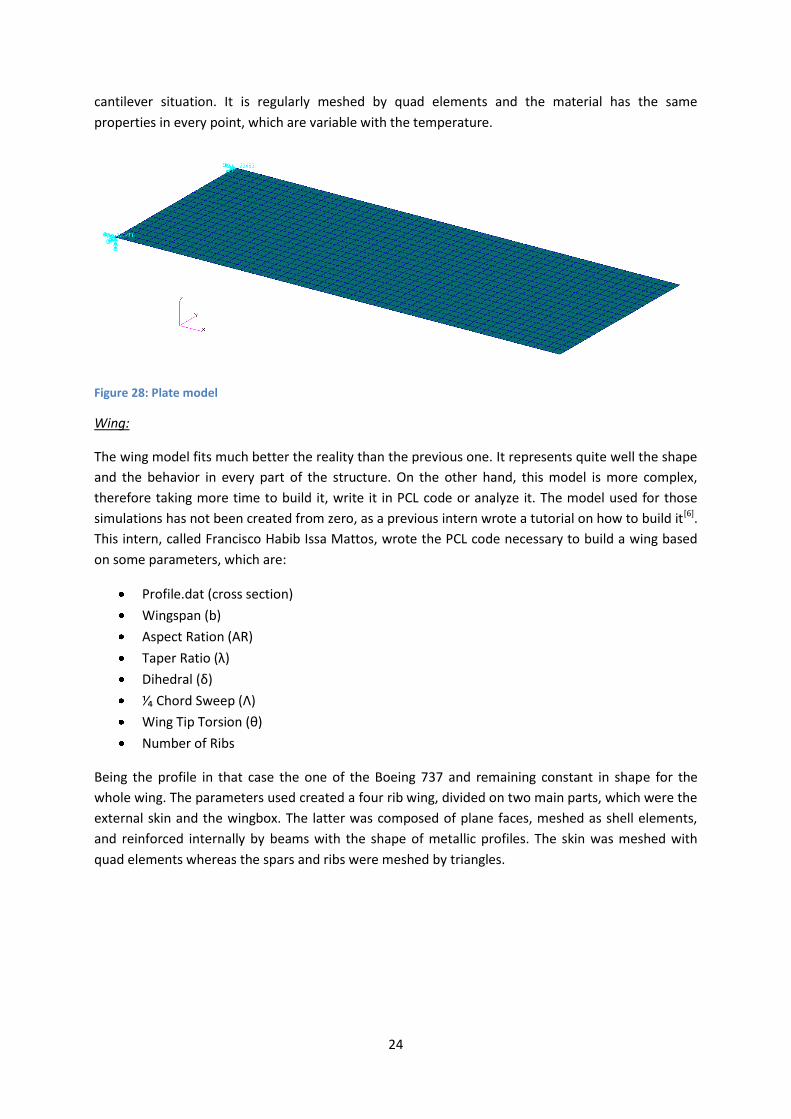
24

cantilever situation. It is regularly meshed by quad elements and the material has the same

properties in every point, which are variable with the temperature.

Figure 28: Plate model

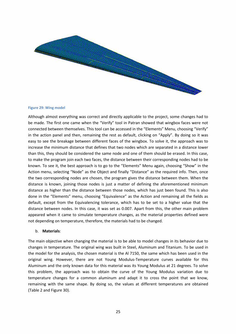
Wing:

The wing model fits much better the reality than the previous one. It represents quite well the shape

and the behavior in every part of the structure. On the other hand, this model is more complex,

therefore taking more time to build it, write it in PCL code or analyze it. The model used for those

simulations has not been created from zero, as a previous intern wrote a tutorial on how to build it[6].

This intern, called Francisco Habib Issa Mattos, wrote the PCL code necessary to build a wing based

on some parameters, which are:

Profile.dat (cross section)

Wingspan (b)

Aspect Ration (AR)

Taper Ratio (λ)

Dihedral (δ)

⅟₄ Chord Sweep (Λ)

Wing Tip Torsion (θ)

Number of Ribs

Being the profile in that case the one of the Boeing 737 and remaining constant in shape for the

whole wing. The parameters used created a four rib wing, divided on two main parts, which were the

external skin and the wingbox. The latter was composed of plane faces, meshed as shell elements,

and reinforced internally by beams with the shape of metallic profiles. The skin was meshed with

quad elements whereas the spars and ribs were meshed by triangles.

25

Figure 29: Wing model

Although almost everything was correct and directly applicable to the project, some changes had to

be made. The first one came when the “Verify” tool in Patran showed that wingbox faces were not

connected between themselves. This tool can be accessed in the “Elements” Menu, choosing “Verify”

in the action panel and then, remaining the rest as default, clicking on “Apply”. By doing so it was

easy to see the breakage between different faces of the wingbox. To solve it, the approach was to

increase the minimum distance that defines that two nodes which are separated in a distance lower

than this, they should be considered the same node and one of them should be erased. In this case,

to make the program join each two faces, the distance between their corresponding nodes had to be

known. To see it, the best approach is to go to the “Elements” Menu again, choosing “Show” in the

Action menu, selecting “Node” as the Object and finally “Distance” as the required info. Then, once

the two corresponding nodes are chosen, the program gives the distance between them. When the

distance is known, joining those nodes is just a matter of defining the aforementioned minimum

distance as higher than the distance between those nodes, which has just been found. This is also

done in the “Elements” menu, choosing “Equivalence” as the Action and remaining all the fields as

default, except from the Equivalencing tolerance, which has to be set to a higher value that the

distance between nodes. In this case, it was set as 0.007. Apart from this, the other main problem

appeared when it came to simulate temperature changes, as the material properties defined were

not depending on temperature, therefore, the materials had to be changed.

b. Materials:

The main objective when changing the material is to be able to model changes in its behavior due to

changes in temperature. The original wing was built in Steel, Aluminum and Titanium. To be used in

the model for the analysis, the chosen material is the Al 7150, the same which has been used in the

original wing. However, there are not Young Modulus-Temperature curves available for this

Aluminum and the only known data for this material was its Young Modulus at 21 degrees. To solve

this problem, the approach was to obtain the curve of the Young Modulus variation due to

temperature changes for a common aluminum and adapt it to cross the point that we know,

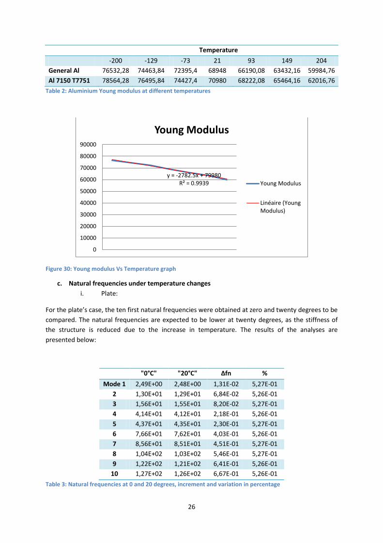
remaining with the same shape. By doing so, the values at different temperatures are obtained

(Table 2 and Figure 30).

26

Temperature

-200 -129 -73 21 93 149 204

General Al 76532,28 74463,84 72395,4 68948 66190,08 63432,16 59984,76

Al 7150 T7751 78564,28 76495,84 74427,4 70980 68222,08 65464,16 62016,76

Table 2: Aluminium Young modulus at different temperatures

Figure 30: Young modulus Vs Temperature graph

c. Natural frequencies under temperature changes

i. Plate:

For the plate’s case, the ten first natural frequencies were obtained at zero and twenty degrees to be

compared. The natural frequencies are expected to be lower at twenty degrees, as the stiffness of

the structure is reduced due to the increase in temperature. The results of the analyses are

presented below:

"0°C" "20°C" Δfn %

Mode 1 2,49E+00 2,48E+00 1,31E-02 5,27E-01

2 1,30E+01 1,29E+01 6,84E-02 5,26E-01

3 1,56E+01 1,55E+01 8,20E-02 5,27E-01

4 4,14E+01 4,12E+01 2,18E-01 5,26E-01

5 4,37E+01 4,35E+01 2,30E-01 5,27E-01

6 7,66E+01 7,62E+01 4,03E-01 5,26E-01

7 8,56E+01 8,51E+01 4,51E-01 5,27E-01

8 1,04E+02 1,03E+02 5,46E-01 5,27E-01

9 1,22E+02 1,21E+02 6,41E-01 5,26E-01

10 1,27E+02 1,26E+02 6,67E-01 5,26E-01

Table 3: Natural frequencies at 0 and 20 degrees, increment and variation in percentage

y = -2782.5x + 79980 R² = 0.9939

0

10000

20000

30000

40000

50000

60000

70000

80000

90000

Young Modulus

Young Modulus

Linéaire (YoungModulus)

27

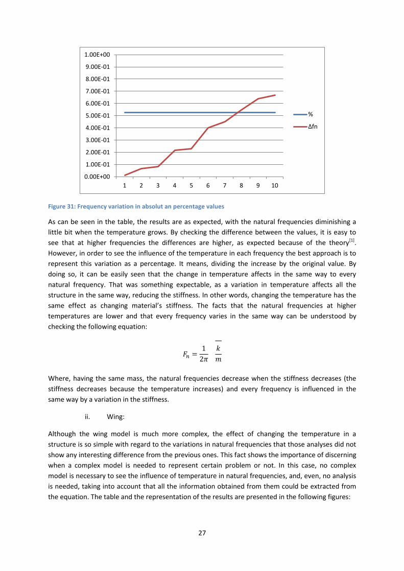
Figure 31: Frequency variation in absolut an percentage values

As can be seen in the table, the results are as expected, with the natural frequencies diminishing a

little bit when the temperature grows. By checking the difference between the values, it is easy to

see that at higher frequencies the differences are higher, as expected because of the theory[1].

However, in order to see the influence of the temperature in each frequency the best approach is to

represent this variation as a percentage. It means, dividing the increase by the original value. By

doing so, it can be easily seen that the change in temperature affects in the same way to every

natural frequency. That was something expectable, as a variation in temperature affects all the

structure in the same way, reducing the stiffness. In other words, changing the temperature has the

same effect as changing material’s stiffness. The facts that the natural frequencies at higher

temperatures are lower and that every frequency varies in the same way can be understood by

checking the following equation:

Where, having the same mass, the natural frequencies decrease when the stiffness decreases (the

stiffness decreases because the temperature increases) and every frequency is influenced in the

same way by a variation in the stiffness.

ii. Wing:

Although the wing model is much more complex, the effect of changing the temperature in a

structure is so simple with regard to the variations in natural frequencies that those analyses did not

show any interesting difference from the previous ones. This fact shows the importance of discerning

when a complex model is needed to represent certain problem or not. In this case, no complex

model is necessary to see the influence of temperature in natural frequencies, and, even, no analysis

is needed, taking into account that all the information obtained from them could be extracted from

the equation. The table and the representation of the results are presented in the following figures:

0.00E+00

1.00E-01

2.00E-01

3.00E-01

4.00E-01

5.00E-01

6.00E-01

7.00E-01

8.00E-01

9.00E-01

1.00E+00

1 2 3 4 5 6 7 8 9 10

%

Δfn

28

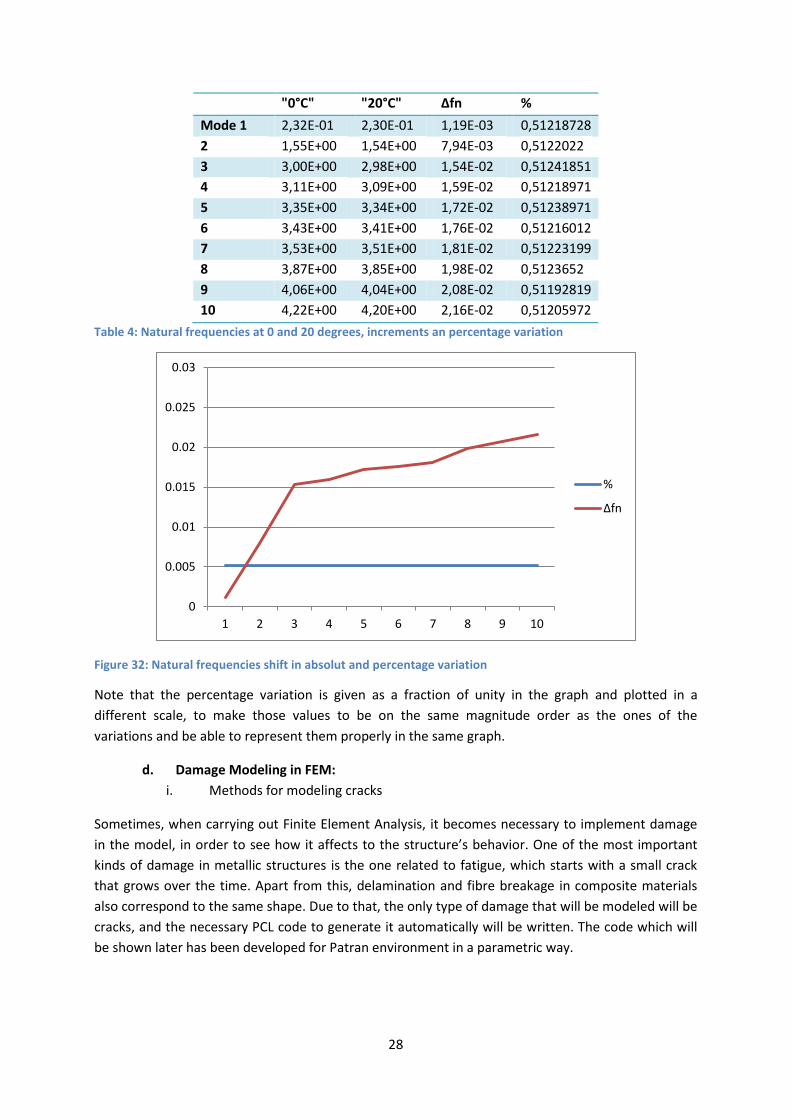
"0°C" "20°C" Δfn %

Mode 1 2,32E-01 2,30E-01 1,19E-03 0,51218728

2 1,55E+00 1,54E+00 7,94E-03 0,5122022

3 3,00E+00 2,98E+00 1,54E-02 0,51241851

4 3,11E+00 3,09E+00 1,59E-02 0,51218971

5 3,35E+00 3,34E+00 1,72E-02 0,51238971

6 3,43E+00 3,41E+00 1,76E-02 0,51216012

7 3,53E+00 3,51E+00 1,81E-02 0,51223199

8 3,87E+00 3,85E+00 1,98E-02 0,5123652

9 4,06E+00 4,04E+00 2,08E-02 0,51192819

10 4,22E+00 4,20E+00 2,16E-02 0,51205972

Table 4: Natural frequencies at 0 and 20 degrees, increments an percentage variation

Figure 32: Natural frequencies shift in absolut and percentage variation

Note that the percentage variation is given as a fraction of unity in the graph and plotted in a

different scale, to make those values to be on the same magnitude order as the ones of the

variations and be able to represent them properly in the same graph.

d. Damage Modeling in FEM:

i. Methods for modeling cracks

Sometimes, when carrying out Finite Element Analysis, it becomes necessary to implement damage

in the model, in order to see how it affects to the structure’s behavior. One of the most important

kinds of damage in metallic structures is the one related to fatigue, which starts with a small crack

that grows over the time. Apart from this, delamination and fibre breakage in composite materials

also correspond to the same shape. Due to that, the only type of damage that will be modeled will be

cracks, and the necessary PCL code to generate it automatically will be written. The code which will

be shown later has been developed for Patran environment in a parametric way.

0

0.005

0.01

0.015

0.02

0.025

0.03

1 2 3 4 5 6 7 8 9 10

%

Δfn

29

The three main methods[1] to simulate cracks in a structure using FEM are:

1. Stiffness Reduction Method (SRM)

2. Kinematics Based Method (KBM), and

3. Duplicate Node Method (DNM) A description of each method is provided below

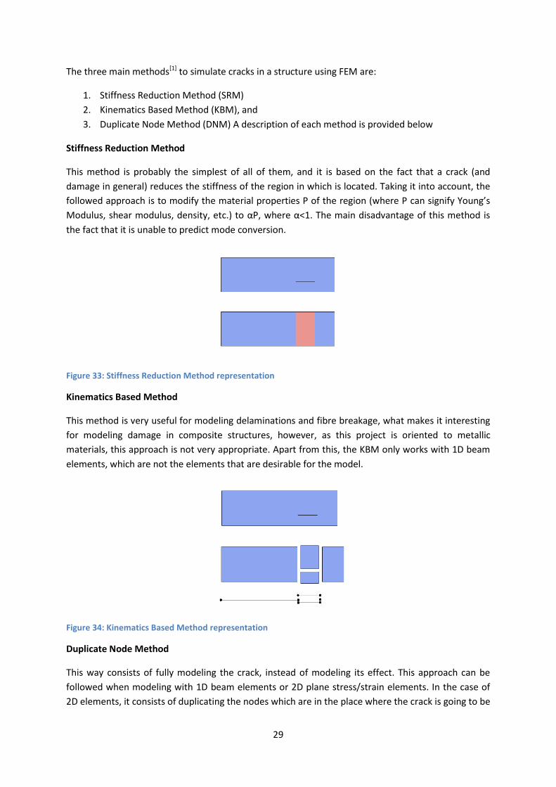
Stiffness Reduction Method

This method is probably the simplest of all of them, and it is based on the fact that a crack (and

damage in general) reduces the stiffness of the region in which is located. Taking it into account, the

followed approach is to modify the material properties P of the region (where P can signify Young’s

Modulus, shear modulus, density, etc.) to αP, where α<1. The main disadvantage of this method is

the fact that it is unable to predict mode conversion.

Figure 33: Stiffness Reduction Method representation

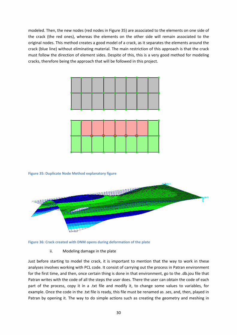
Kinematics Based Method

This method is very useful for modeling delaminations and fibre breakage, what makes it interesting

for modeling damage in composite structures, however, as this project is oriented to metallic

materials, this approach is not very appropriate. Apart from this, the KBM only works with 1D beam

elements, which are not the elements that are desirable for the model.

Figure 34: Kinematics Based Method representation

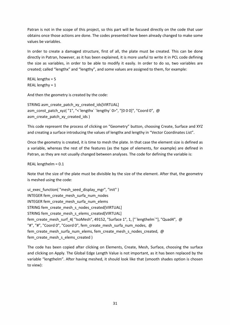
Duplicate Node Method

This way consists of fully modeling the crack, instead of modeling its effect. This approach can be

followed when modeling with 1D beam elements or 2D plane stress/strain elements. In the case of

2D elements, it consists of duplicating the nodes which are in the place where the crack is going to be

30

modeled. Then, the new nodes (red nodes in Figure 35) are associated to the elements on one side of

the crack (the red ones), whereas the elements on the other side will remain associated to the

original nodes. This method creates a good model of a crack, as it separates the elements around the

crack (blue line) without eliminating material. The main restriction of this approach is that the crack

must follow the direction of element sides. Despite of this, this is a very good method for modeling

cracks, therefore being the approach that will be followed in this project.

Figure 35: Duplicate Node Method explanatory figure

Figure 36: Crack created with DNM opens during deformation of the plate

ii. Modeling damage in the plate

Just before starting to model the crack, it is important to mention that the way to work in these

analyses involves working with PCL code. It consist of carrying out the process in Patran environment

for the first time, and then, once certain thing is done in that environment, go to the .db.jou file that

Patran writes with the code of all the steps the user does. There the user can obtain the code of each

part of the process, copy it in a .txt file and modify it, to change some values to variables, for

example. Once the code in the .txt file is ready, this file must be renamed as .ses, and, then, played in

Patran by opening it. The way to do simple actions such as creating the geometry and meshing in

31

Patran is not in the scope of this project, so this part will be focused directly on the code that user

obtains once those actions are done. The codes presented have been already changed to make some

values be variables.

In order to create a damaged structure, first of all, the plate must be created. This can be done

directly in Patran, however, as it has been explained, it is more useful to write it in PCL code defining

the size as variables, in order to be able to modify it easily. In order to do so, two variables are

created; called “lengthx” and “lengthy”, and some values are assigned to them, for example:

REAL lengthx = 5

REAL lengthy = 1

And then the geometry is created by the code:

STRING asm_create_patch_xy_created_ids[VIRTUAL]

asm_const_patch_xyz( "1", "<`lengthx` `lengthy` 0>", "[0 0 0]", "Coord 0", @

asm_create_patch_xy_created_ids )

This code represent the process of clicking on “Geometry” button, choosing Create, Surface and XYZ

and creating a surface introducing the values of lengthx and lengthy in “Vector Coordinates List”.

Once the geometry is created, it is time to mesh the plate. In that case the element size is defined as

a variable, whereas the rest of the features (as the type of elements, for example) are defined in

Patran, as they are not usually changed between analyses. The code for defining the variable is:

REAL lengthelm = 0.1

Note that the size of the plate must be divisible by the size of the element. After that, the geometry

is meshed using the code:

ui_exec_function( "mesh_seed_display_mgr", "init" )

INTEGER fem_create_mesh_surfa_num_nodes

INTEGER fem_create_mesh_surfa_num_elems

STRING fem_create_mesh_s_nodes_created[VIRTUAL]

STRING fem_create_mesh_s_elems_created[VIRTUAL]

fem_create_mesh_surf_4( "IsoMesh", 49152, "Surface 1", 1, ["`lengthelm`"], "Quad4", @

"#", "#", "Coord 0", "Coord 0", fem_create_mesh_surfa_num_nodes, @

fem_create_mesh_surfa_num_elems, fem_create_mesh_s_nodes_created, @

fem_create_mesh_s_elems_created )

The code has been copied after clicking on Elements, Create, Mesh, Surface, choosing the surface

and clicking on Apply. The Global Edge Length Value is not important, as it has been replaced by the

variable “lengthelm”. After having meshed, it should look like that (smooth shades option is chosen

to view):

32

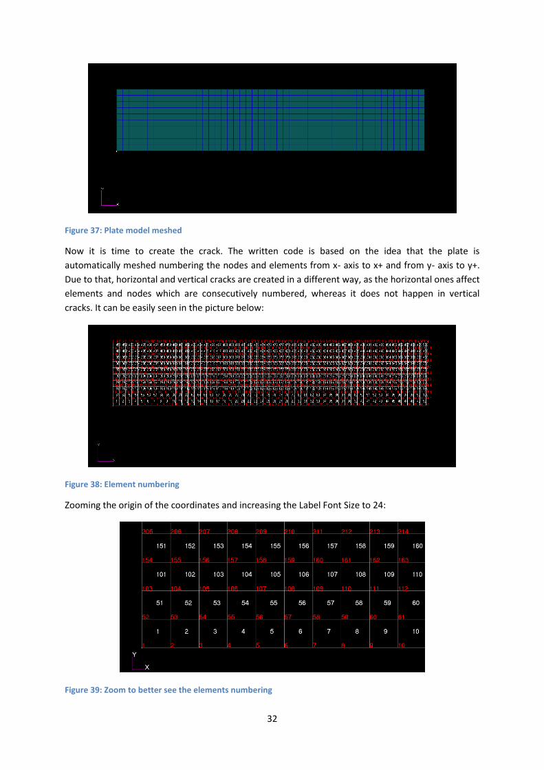
Figure 37: Plate model meshed

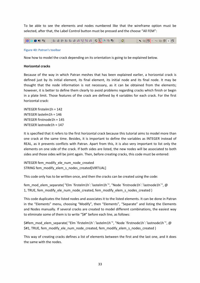
Now it is time to create the crack. The written code is based on the idea that the plate is

automatically meshed numbering the nodes and elements from x- axis to x+ and from y- axis to y+.

Due to that, horizontal and vertical cracks are created in a different way, as the horizontal ones affect

elements and nodes which are consecutively numbered, whereas it does not happen in vertical

cracks. It can be easily seen in the picture below:

Figure 38: Element numbering

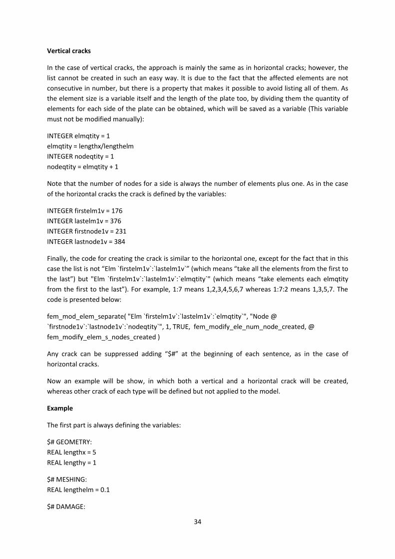
Zooming the origin of the coordinates and increasing the Label Font Size to 24:

Figure 39: Zoom to better see the elements numbering

33

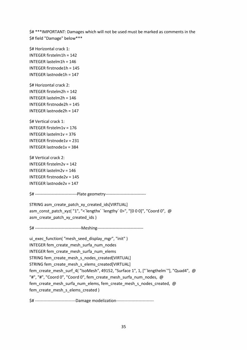
To be able to see the elements and nodes numbered like that the wireframe option must be

selected, after that, the Label Control button must be pressed and the choose “All FEM”:

Figure 40: Patran’s toolbar

Now how to model the crack depending on its orientation is going to be explained below.

Horizontal cracks

Because of the way in which Patran meshes that has been explained earlier, a horizontal crack is

defined just by its initial element, its final element, its initial node and its final node. It may be

thought that the node information is not necessary, as it can be obtained from the elements;

however, it is better to define them clearly to avoid problems regarding cracks which finish or begin

in a plate limit. Those features of the crack are defined by 4 variables for each crack. For the first

horizontal crack:

INTEGER firstelm1h = 142

INTEGER lastelm1h = 146

INTEGER firstnode1h = 145

INTEGER lastnode1h = 147

It is specified that it refers to the first horizontal crack because this tutorial aims to model more than

one crack at the same time. Besides, it is important to define the variables as INTEGER instead of

REAL, as it prevents conflicts with Patran. Apart from this, it is also very important to list only the

elements on one side of the crack. If both sides are listed, the new nodes will be associated to both

sides and those sides will be joint again. Then, before creating cracks, this code must be entered:

INTEGER fem_modify_ele_num_node_created

STRING fem_modify_elem_s_nodes_created[VIRTUAL]

This code only has to be written once, and then the cracks can be created using the code:

fem_mod_elem_separate( "Elm `firstelm1h`:`lastelm1h`", "Node `firstnode1h`:`lastnode1h`", @

1, TRUE, fem_modify_ele_num_node_created, fem_modify_elem_s_nodes_created )

This code duplicates the listed nodes and associates it to the listed elements. It can be done in Patran

in the “Elements” menu, choosing “Modify”, then “Elements”, “Separate” and listing the Elements

and Nodes manually. If several cracks are created to model different combinations, the easiest way

to eliminate some of them is to write “$#” before each line, as follows:

$#fem_mod_elem_separate( "Elm `firstelm1h`:`lastelm1h`", "Node `firstnode1h`:`lastnode1h`", @

$#1, TRUE, fem_modify_ele_num_node_created, fem_modify_elem_s_nodes_created )

This way of creating cracks defines a list of elements between the first and the last one, and it does

the same with the nodes.

34

Vertical cracks

In the case of vertical cracks, the approach is mainly the same as in horizontal cracks; however, the

list cannot be created in such an easy way. It is due to the fact that the affected elements are not

consecutive in number, but there is a property that makes it possible to avoid listing all of them. As

the element size is a variable itself and the length of the plate too, by dividing them the quantity of

elements for each side of the plate can be obtained, which will be saved as a variable (This variable

must not be modified manually):

INTEGER elmqtity = 1

elmqtity = lengthx/lengthelm

INTEGER nodeqtity = 1

nodeqtity = elmqtity + 1

Note that the number of nodes for a side is always the number of elements plus one. As in the case

of the horizontal cracks the crack is defined by the variables:

INTEGER firstelm1v = 176

INTEGER lastelm1v = 376

INTEGER firstnode1v = 231

INTEGER lastnode1v = 384

Finally, the code for creating the crack is similar to the horizontal one, except for the fact that in this

case the list is not “Elm `firstelm1v`:`lastelm1v`” (which means “take all the elements from the first to

the last”) but "Elm `firstelm1v`:`lastelm1v`:èlmqtity`" (which means “take elements each elmqtity

from the first to the last”). For example, 1:7 means 1,2,3,4,5,6,7 whereas 1:7:2 means 1,3,5,7. The

code is presented below:

fem_mod_elem_separate( "Elm `firstelm1v`:`lastelm1v`:èlmqtity`", "Node @

`firstnode1v`:`lastnode1v`:`nodeqtity`", 1, TRUE, fem_modify_ele_num_node_created, @

fem_modify_elem_s_nodes_created )

Any crack can be suppressed adding “$#” at the beginning of each sentence, as in the case of

horizontal cracks.

Now an example will be show, in which both a vertical and a horizontal crack will be created,

whereas other crack of each type will be defined but not applied to the model.

Example

The first part is always defining the variables:

$# GEOMETRY:

REAL lengthx = 5

REAL lengthy = 1

$# MESHING:


$# DAMAGE:

35

$# ***IMPORTANT: Damages which will not be used must be marked as comments in the

$# field "Damage" below***

$# Horizontal crack 1:










$# Vertical crack 1:





$# Vertical crack 2:





$# ------------------------------Plate geometry-----------------------------




$# ---------------------------------Meshing---------------------------------










$# -----------------------------Damage modelization---------------------------

36



$# Horizontal cracks:

fem_mod_elem_separate( "Elm `firstelm1h`:`lastelm1h`", "Node `firstnode1h`:`lastnode1h`", @

1, TRUE, fem_modify_ele_num_node_created, fem_modify_elem_s_nodes_created )

$#fem_mod_elem_separate( "Elm `firstelm2h`:`lastelm2h`", "Node `firstnode2h`:`lastnode2h`", @

$#1, TRUE, fem_modify_ele_num_node_created, fem_modify_elem_s_nodes_created )

$# Vertical cracks:

fem_mod_elem_separate( "Elm `firstelm1v`:`lastelm1v`:èlmqtity`", "Node @

`firstnode1v`:`lastnode1v`:`nodeqtity`", 1, TRUE, fem_modify_ele_num_node_created, @


$#fem_mod_elem_separate( "Elm `firstelm2v`:`lastelm2v`:èlmqtity`", "Node @

$#`firstnode2v`:`lastnode2v`:`nodeqtity`", 1, TRUE, fem_modify_ele_num_node_created, @

$#fem_modify_elem_s_nodes_created )

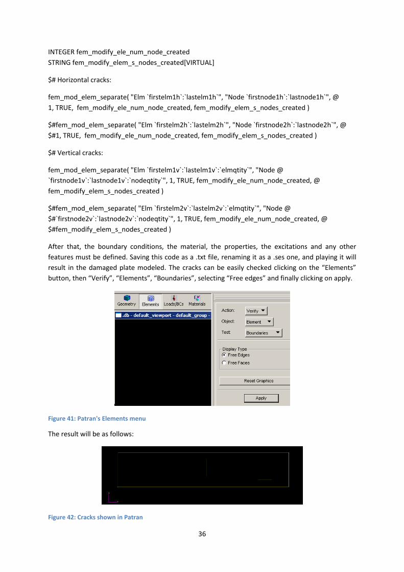
After that, the boundary conditions, the material, the properties, the excitations and any other

features must be defined. Saving this code as a .txt file, renaming it as a .ses one, and playing it will

result in the damaged plate modeled. The cracks can be easily checked clicking on the “Elements”

button, then “Verify”, “Elements”, “Boundaries”, selecting “Free edges” and finally clicking on apply.

Figure 41: Patran's Elements menu

The result will be as follows:

Figure 42: Cracks shown in Patran

37

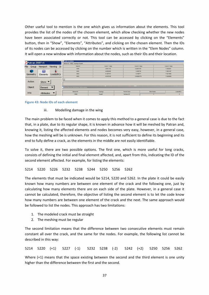
Other useful tool to mention is the one which gives us information about the elements. This tool

provides the list of the nodes of the chosen element, which allow checking whether the new nodes

have been associated correctly or not. This tool can be accessed by clicking on the “Elements”

button, then in “Show”, “Elements”, “Attributes”, and clicking on the chosen element. Then the IDs

of its nodes can be accessed by clicking on the number which is written in the “Elem Nodes” column.

It will open a new window with information about the nodes, such as their IDs and their location.

Figure 43: Node IDs of each element

iii. Modelling damage in the wing

The main problem to be faced when it comes to apply this method to a general case is due to the fact

that, in a plate, due to its regular shape, it is known in advance how it will be meshed by Patran and,

knowing it, listing the affected elements and nodes becomes very easy, however, in a general case,

how the meshing will be is unknown. For this reason, it is not sufficient to define its beginning and its

end to fully define a crack, as the elements in the middle are not easily identifiable.

To solve it, there are two possible options. The first one, which is more useful for long cracks,

consists of defining the initial and final element affected, and, apart from this, indicating the ID of the

second element affected. For example, for listing the elements:

5214 5220 5226 5232 5238 5244 5250 5256 5262

The elements that must be indicated would be 5214, 5220 and 5262. In the plate it could be easily

known how many numbers are between one element of the crack and the following one, just by

calculating how many elements there are on each side of the plate. However, in a general case it

cannot be calculated, therefore, the objective of listing the second element is to let the code know

how many numbers are between one element of the crack and the next. The same approach would

be followed to list the nodes. This approach has two limitations:

1. The modeled crack must be straight

2. The meshing must be regular

The second limitation means that the difference between two consecutive elements must remain

constant all over the crack, and the same for the nodes. For example, the following list cannot be

described in this way:

5214 5220 (+1) 5227 (-1) 5232 5238 (-2) 5242 (+2) 5250 5256 5262

Where (+1) means that the space existing between the second and the third element is one unity

higher than the difference between the first and the second.

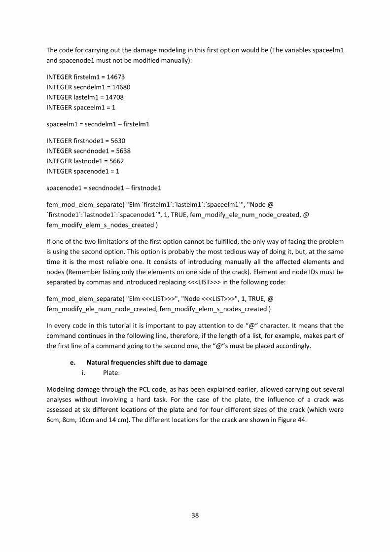
38

The code for carrying out the damage modeling in this first option would be (The variables spaceelm1

and spacenode1 must not be modified manually):

INTEGER firstelm1 = 14673

INTEGER secndelm1 = 14680

INTEGER lastelm1 = 14708

INTEGER spaceelm1 = 1

spaceelm1 = secndelm1 – firstelm1

INTEGER firstnode1 = 5630

INTEGER secndnode1 = 5638

INTEGER lastnode1 = 5662

INTEGER spacenode1 = 1

spacenode1 = secndnode1 – firstnode1

fem_mod_elem_separate( "Elm `firstelm1`:`lastelm1`:`spaceelm1`", "Node @

`firstnode1`:`lastnode1`:`spacenode1`", 1, TRUE, fem_modify_ele_num_node_created, @


If one of the two limitations of the first option cannot be fulfilled, the only way of facing the problem

is using the second option. This option is probably the most tedious way of doing it, but, at the same

time it is the most reliable one. It consists of introducing manually all the affected elements and

nodes (Remember listing only the elements on one side of the crack). Element and node IDs must be

separated by commas and introduced replacing <<<LIST>>> in the following code:

fem_mod_elem_separate( "Elm <<<LIST>>>", "Node <<<LIST>>>", 1, TRUE, @

fem_modify_ele_num_node_created, fem_modify_elem_s_nodes_created )

In every code in this tutorial it is important to pay attention to de “@” character. It means that the

command continues in the following line, therefore, if the length of a list, for example, makes part of

the first line of a command going to the second one, the “@”s must be placed accordingly.

e. Natural frequencies shift due to damage

i. Plate:

Modeling damage through the PCL code, as has been explained earlier, allowed carrying out several

analyses without involving a hard task. For the case of the plate, the influence of a crack was

assessed at six different locations of the plate and for four different sizes of the crack (which were

6cm, 8cm, 10cm and 14 cm). The different locations for the crack are shown in Figure 44.

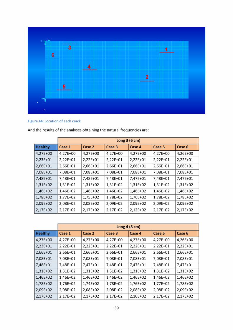
39

Figure 44: Location of each crack

And the results of the analyses obtaining the natural frequencies are:

Long 3 (6 cm)

Healthy Case 1 Case 2 Case 3 Case 4 Case 5 Case 6

4,27E+00 4,27E+00 4,27E+00 4,27E+00 4,27E+00 4,27E+00 4,26E+00

2,23E+01 2,22E+01 2,22E+01 2,22E+01 2,22E+01 2,22E+01 2,22E+01

2,66E+01 2,66E+01 2,66E+01 2,66E+01 2,66E+01 2,66E+01 2,66E+01

7,08E+01 7,08E+01 7,08E+01 7,08E+01 7,08E+01 7,08E+01 7,08E+01

7,48E+01 7,48E+01 7,48E+01 7,48E+01 7,47E+01 7,48E+01 7,47E+01

1,31E+02 1,31E+02 1,31E+02 1,31E+02 1,31E+02 1,31E+02 1,31E+02

1,46E+02 1,46E+02 1,46E+02 1,46E+02 1,46E+02 1,46E+02 1,46E+02

1,78E+02 1,77E+02 1,75E+02 1,78E+02 1,76E+02 1,78E+02 1,78E+02

2,09E+02 2,08E+02 2,08E+02 2,09E+02 2,09E+02 2,09E+02 2,09E+02

2,17E+02 2,17E+02 2,17E+02 2,17E+02 2,12E+02 2,17E+02 2,17E+02

Long 4 (8 cm)


4,27E+00 4,27E+00 4,27E+00 4,27E+00 4,27E+00 4,27E+00 4,26E+00

2,23E+01 2,22E+01 2,22E+01 2,22E+01 2,22E+01 2,22E+01 2,22E+01

2,66E+01 2,66E+01 2,66E+01 2,66E+01 2,66E+01 2,66E+01 2,66E+01

7,08E+01 7,08E+01 7,08E+01 7,08E+01 7,08E+01 7,08E+01 7,08E+01

7,48E+01 7,48E+01 7,47E+01 7,48E+01 7,47E+01 7,48E+01 7,47E+01

1,31E+02 1,31E+02 1,31E+02 1,31E+02 1,31E+02 1,31E+02 1,31E+02

1,46E+02 1,46E+02 1,46E+02 1,46E+02 1,46E+02 1,46E+02 1,46E+02

1,78E+02 1,76E+02 1,74E+02 1,78E+02 1,76E+02 1,77E+02 1,78E+02

2,09E+02 2,08E+02 2,08E+02 2,08E+02 2,08E+02 2,08E+02 2,09E+02

2,17E+02 2,17E+02 2,17E+02 2,17E+02 2,10E+02 2,17E+02 2,17E+02

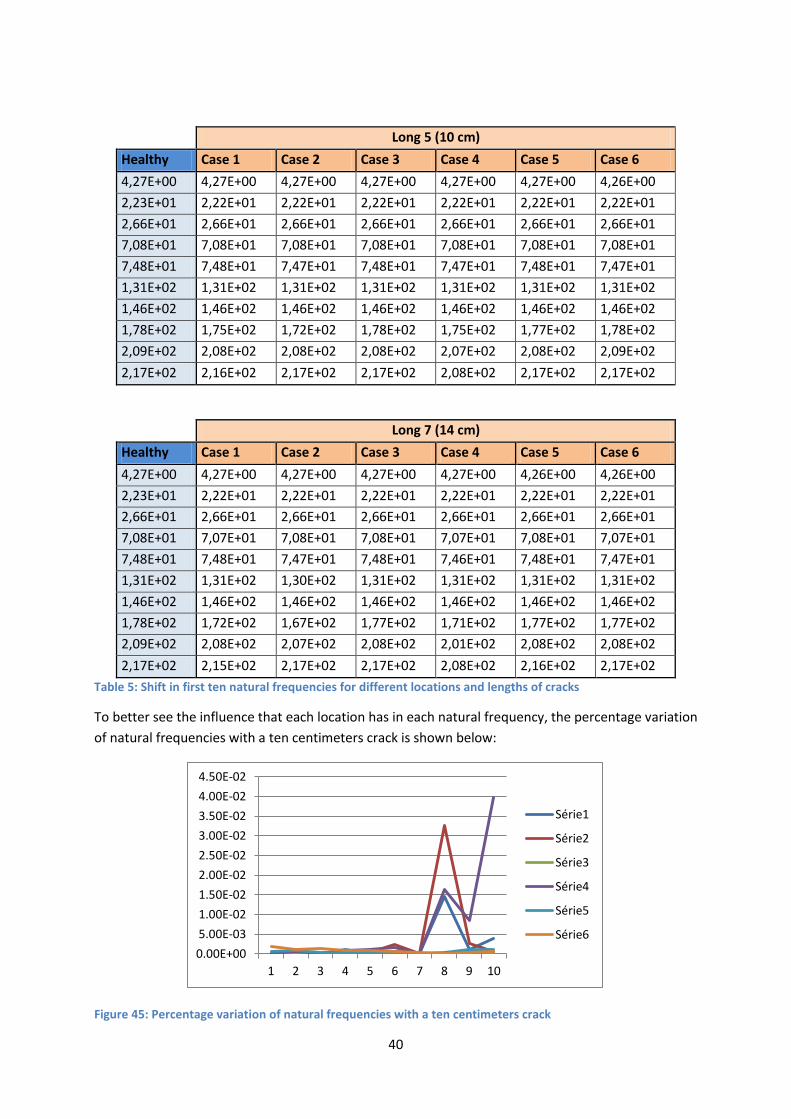
40

Long 5 (10 cm)


4,27E+00 4,27E+00 4,27E+00 4,27E+00 4,27E+00 4,27E+00 4,26E+00

2,23E+01 2,22E+01 2,22E+01 2,22E+01 2,22E+01 2,22E+01 2,22E+01

2,66E+01 2,66E+01 2,66E+01 2,66E+01 2,66E+01 2,66E+01 2,66E+01

7,08E+01 7,08E+01 7,08E+01 7,08E+01 7,08E+01 7,08E+01 7,08E+01

7,48E+01 7,48E+01 7,47E+01 7,48E+01 7,47E+01 7,48E+01 7,47E+01

1,31E+02 1,31E+02 1,31E+02 1,31E+02 1,31E+02 1,31E+02 1,31E+02

1,46E+02 1,46E+02 1,46E+02 1,46E+02 1,46E+02 1,46E+02 1,46E+02

1,78E+02 1,75E+02 1,72E+02 1,78E+02 1,75E+02 1,77E+02 1,78E+02

2,09E+02 2,08E+02 2,08E+02 2,08E+02 2,07E+02 2,08E+02 2,09E+02

2,17E+02 2,16E+02 2,17E+02 2,17E+02 2,08E+02 2,17E+02 2,17E+02

Long 7 (14 cm)


4,27E+00 4,27E+00 4,27E+00 4,27E+00 4,27E+00 4,26E+00 4,26E+00

2,23E+01 2,22E+01 2,22E+01 2,22E+01 2,22E+01 2,22E+01 2,22E+01

2,66E+01 2,66E+01 2,66E+01 2,66E+01 2,66E+01 2,66E+01 2,66E+01

7,08E+01 7,07E+01 7,08E+01 7,08E+01 7,07E+01 7,08E+01 7,07E+01

7,48E+01 7,48E+01 7,47E+01 7,48E+01 7,46E+01 7,48E+01 7,47E+01

1,31E+02 1,31E+02 1,30E+02 1,31E+02 1,31E+02 1,31E+02 1,31E+02

1,46E+02 1,46E+02 1,46E+02 1,46E+02 1,46E+02 1,46E+02 1,46E+02

1,78E+02 1,72E+02 1,67E+02 1,77E+02 1,71E+02 1,77E+02 1,77E+02

2,09E+02 2,08E+02 2,07E+02 2,08E+02 2,01E+02 2,08E+02 2,08E+02

2,17E+02 2,15E+02 2,17E+02 2,17E+02 2,08E+02 2,16E+02 2,17E+02

Table 5: Shift in first ten natural frequencies for different locations and lengths of cracks

To better see the influence that each location has in each natural frequency, the percentage variation

of natural frequencies with a ten centimeters crack is shown below:

Figure 45: Percentage variation of natural frequencies with a ten centimeters crack

0.00E+00

5.00E-03

1.00E-02

1.50E-02

2.00E-02

2.50E-02

3.00E-02

3.50E-02

4.00E-02

4.50E-02

1 2 3 4 5 6 7 8 9 10

Série1

Série2

Série3

Série4

Série5

Série6

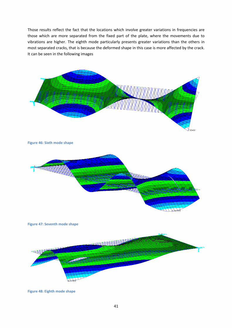
41

Those results reflect the fact that the locations which involve greater variations in frequencies are

those which are more separated from the fixed part of the plate, where the movements due to

vibrations are higher. The eighth mode particularly presents greater variations than the others in

most separated cracks, that is because the deformed shape in this case is more affected by the crack.

It can be seen in the following images

Figure 46: Sixth mode shape

Figure 47: Seventh mode shape

Figure 48: Eighth mode shape

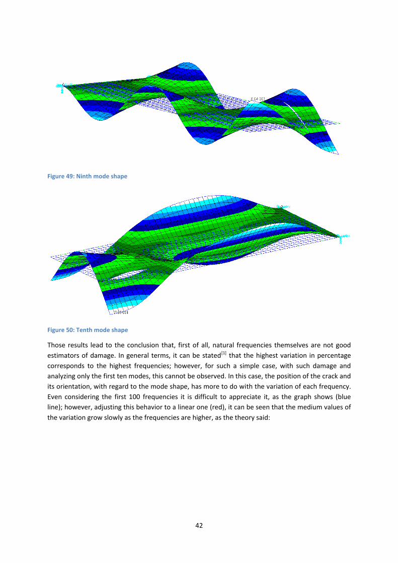
42

Figure 49: Ninth mode shape

Figure 50: Tenth mode shape

Those results lead to the conclusion that, first of all, natural frequencies themselves are not good

estimators of damage. In general terms, it can be stated[1] that the highest variation in percentage

corresponds to the highest frequencies; however, for such a simple case, with such damage and

analyzing only the first ten modes, this cannot be observed. In this case, the position of the crack and

its orientation, with regard to the mode shape, has more to do with the variation of each frequency.

Even considering the first 100 frequencies it is difficult to appreciate it, as the graph shows (blue

line); however, adjusting this behavior to a linear one (red), it can be seen that the medium values of

the variation grow slowly as the frequencies are higher, as the theory said:

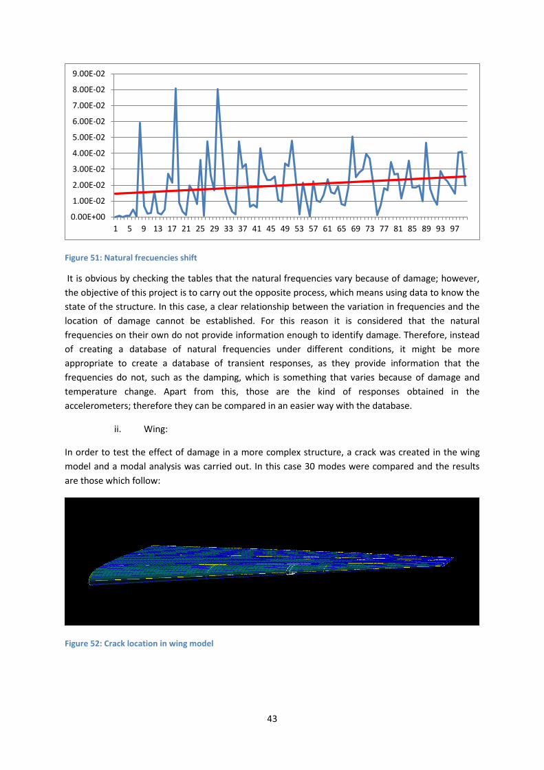
43

Figure 51: Natural frecuencies shift

It is obvious by checking the tables that the natural frequencies vary because of damage; however,

the objective of this project is to carry out the opposite process, which means using data to know the

state of the structure. In this case, a clear relationship between the variation in frequencies and the

location of damage cannot be established. For this reason it is considered that the natural

frequencies on their own do not provide information enough to identify damage. Therefore, instead

of creating a database of natural frequencies under different conditions, it might be more

appropriate to create a database of transient responses, as they provide information that the

frequencies do not, such as the damping, which is something that varies because of damage and

temperature change. Apart from this, those are the kind of responses obtained in the

accelerometers; therefore they can be compared in an easier way with the database.

ii. Wing:

In order to test the effect of damage in a more complex structure, a crack was created in the wing

model and a modal analysis was carried out. In this case 30 modes were compared and the results

are those which follow:

Figure 52: Crack location in wing model

0.00E+00

1.00E-02

2.00E-02

3.00E-02

4.00E-02

5.00E-02

6.00E-02

7.00E-02

8.00E-02

9.00E-02

1 5 9 13 17 21 25 29 33 37 41 45 49 53 57 61 65 69 73 77 81 85 89 93 97

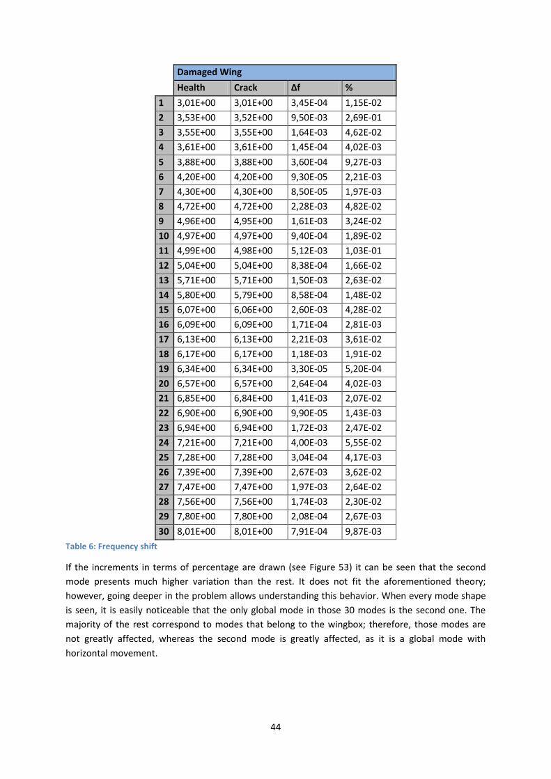
44

Damaged Wing

Health Crack Δf %

1 3,01E+00 3,01E+00 3,45E-04 1,15E-02

2 3,53E+00 3,52E+00 9,50E-03 2,69E-01

3 3,55E+00 3,55E+00 1,64E-03 4,62E-02

4 3,61E+00 3,61E+00 1,45E-04 4,02E-03

5 3,88E+00 3,88E+00 3,60E-04 9,27E-03

6 4,20E+00 4,20E+00 9,30E-05 2,21E-03

7 4,30E+00 4,30E+00 8,50E-05 1,97E-03

8 4,72E+00 4,72E+00 2,28E-03 4,82E-02

9 4,96E+00 4,95E+00 1,61E-03 3,24E-02

10 4,97E+00 4,97E+00 9,40E-04 1,89E-02

11 4,99E+00 4,98E+00 5,12E-03 1,03E-01

12 5,04E+00 5,04E+00 8,38E-04 1,66E-02

13 5,71E+00 5,71E+00 1,50E-03 2,63E-02

14 5,80E+00 5,79E+00 8,58E-04 1,48E-02

15 6,07E+00 6,06E+00 2,60E-03 4,28E-02

16 6,09E+00 6,09E+00 1,71E-04 2,81E-03

17 6,13E+00 6,13E+00 2,21E-03 3,61E-02

18 6,17E+00 6,17E+00 1,18E-03 1,91E-02

19 6,34E+00 6,34E+00 3,30E-05 5,20E-04

20 6,57E+00 6,57E+00 2,64E-04 4,02E-03

21 6,85E+00 6,84E+00 1,41E-03 2,07E-02

22 6,90E+00 6,90E+00 9,90E-05 1,43E-03

23 6,94E+00 6,94E+00 1,72E-03 2,47E-02

24 7,21E+00 7,21E+00 4,00E-03 5,55E-02

25 7,28E+00 7,28E+00 3,04E-04 4,17E-03

26 7,39E+00 7,39E+00 2,67E-03 3,62E-02

27 7,47E+00 7,47E+00 1,97E-03 2,64E-02

28 7,56E+00 7,56E+00 1,74E-03 2,30E-02

29 7,80E+00 7,80E+00 2,08E-04 2,67E-03

30 8,01E+00 8,01E+00 7,91E-04 9,87E-03

Table 6: Frequency shift

If the increments in terms of percentage are drawn (see Figure 53) it can be seen that the second

mode presents much higher variation than the rest. It does not fit the aforementioned theory;

however, going deeper in the problem allows understanding this behavior. When every mode shape

is seen, it is easily noticeable that the only global mode in those 30 modes is the second one. The

majority of the rest correspond to modes that belong to the wingbox; therefore, those modes are

not greatly affected, whereas the second mode is greatly affected, as it is a global mode with

horizontal movement.

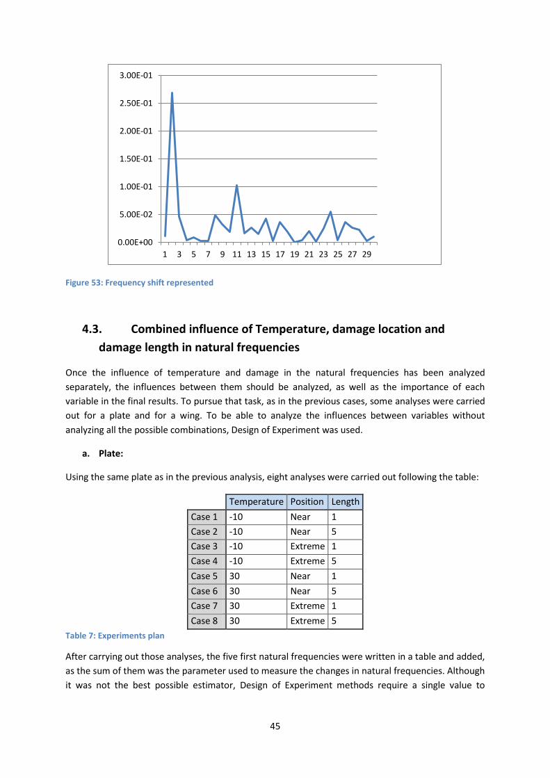
45

Figure 53: Frequency shift represented

4.3. Combined influence of Temperature, damage location and

damage length in natural frequencies

Once the influence of temperature and damage in the natural frequencies has been analyzed

separately, the influences between them should be analyzed, as well as the importance of each

variable in the final results. To pursue that task, as in the previous cases, some analyses were carried

out for a plate and for a wing. To be able to analyze the influences between variables without

analyzing all the possible combinations, Design of Experiment was used.

a. Plate:

Using the same plate as in the previous analysis, eight analyses were carried out following the table:

Temperature Position Length

Case 1 -10 Near 1

Case 2 -10 Near 5

Case 3 -10 Extreme 1

Case 4 -10 Extreme 5

Case 5 30 Near 1

Case 6 30 Near 5

Case 7 30 Extreme 1

Case 8 30 Extreme 5

Table 7: Experiments plan

After carrying out those analyses, the five first natural frequencies were written in a table and added,

as the sum of them was the parameter used to measure the changes in natural frequencies. Although

it was not the best possible estimator, Design of Experiment methods require a single value to

0.00E+00

5.00E-02

1.00E-01

1.50E-01

2.00E-01

2.50E-01

3.00E-01

1 3 5 7 9 11 13 15 17 19 21 23 25 27 29

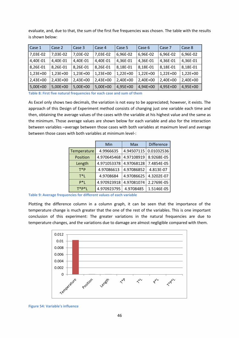
46

evaluate, and, due to that, the sum of the first five frequencies was chosen. The table with the results

is shown below:

Case 1 Case 2 Case 3 Case 4 Case 5 Case 6 Case 7 Case 8

7,03E-02 7,03E-02 7,03E-02 7,03E-02 6,96E-02 6,96E-02 6,96E-02 6,96E-02

4,40E-01 4,40E-01 4,40E-01 4,40E-01 4,36E-01 4,36E-01 4,36E-01 4,36E-01

8,26E-01 8,26E-01 8,26E-01 8,26E-01 8,18E-01 8,18E-01 8,18E-01 8,18E-01

1,23E+00 1,23E+00 1,23E+00 1,23E+00 1,22E+00 1,22E+00 1,22E+00 1,22E+00

2,43E+00 2,43E+00 2,43E+00 2,43E+00 2,40E+00 2,40E+00 2,40E+00 2,40E+00

5,00E+00 5,00E+00 5,00E+00 5,00E+00 4,95E+00 4,94E+00 4,95E+00 4,95E+00

Table 8: First five natural frequencies for each case and sum of them

As Excel only shows two decimals, the variation is not easy to be appreciated; however, it exists. The

approach of this Design of Experiment method consists of changing just one variable each time and

then, obtaining the average values of the cases with the variable at his highest value and the same as

the minimum. Those average values are shown below for each variable and also for the interaction

between variables –average between those cases with both variables at maximum level and average

between those cases with both variables at minimum level-:

Min Max Difference

Temperature 4.9966635 4.94507115 0.01032536

Position 4.970645468 4.97108919 8.9268E-05

Length 4.971053378 4.97068128 7.4854E-05

T*P 4.97086613 4.97086852 4.813E-07

T*L 4.9708684 4.97086625 4.3202E-07

P*L 4.970923918 4.97081074 2.2769E-05

T*P*L 4.970923795 4.9708485 1.5146E-05

Table 9: Average frequencies for different values of each variable

Plotting the difference column in a column graph, it can be seen that the importance of the

temperature change is much greater that the one of the rest of the variables. This is one important

conclusion of this experiment: The greater variations in the natural frequencies are due to

temperature changes, and the variations due to damage are almost negligible compared with them.

Figure 54: Variable's influence

0

0.002

0.004

0.006

0.008

0.01

0.012

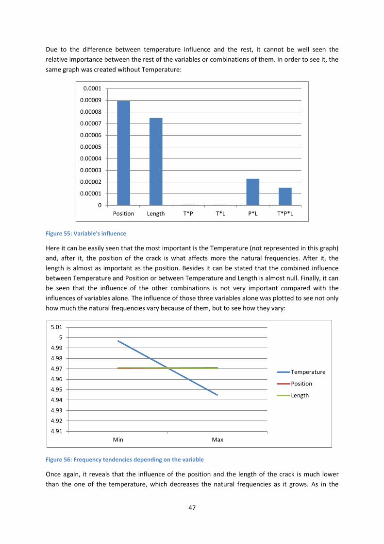
47

Due to the difference between temperature influence and the rest, it cannot be well seen the

relative importance between the rest of the variables or combinations of them. In order to see it, the

same graph was created without Temperature:


Here it can be easily seen that the most important is the Temperature (not represented in this graph)

and, after it, the position of the crack is what affects more the natural frequencies. After it, the

length is almost as important as the position. Besides it can be stated that the combined influence

between Temperature and Position or between Temperature and Length is almost null. Finally, it can

be seen that the influence of the other combinations is not very important compared with the

influences of variables alone. The influence of those three variables alone was plotted to see not only

how much the natural frequencies vary because of them, but to see how they vary:

Figure 56: Frequency tendencies depending on the variable

Once again, it reveals that the influence of the position and the length of the crack is much lower

than the one of the temperature, which decreases the natural frequencies as it grows. As in the

0

0.00001

0.00002

0.00003

0.00004

0.00005

0.00006

0.00007

0.00008

0.00009

0.0001

Position Length T*P T*L P*L T*P*L

4.91

4.92

4.93

4.94

4.95

4.96

4.97

4.98

4.99

5

5.01

Min Max

Temperature

Position

Length

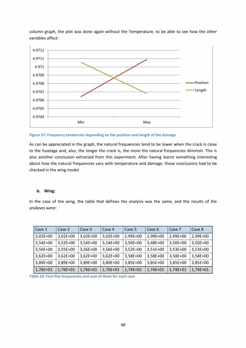
48

column graph, the plot was done again without the Temperature, to be able to see how the other

variables affect:

Figure 57: Frequency tendencies depending on the position and length of the damage

As can be appreciated in the graph, the natural frequencies tend to be lower when the crack is close

to the fuselage and, also, the longer the crack is, the more the natural frequencies diminish. This is

also another conclusion extracted from this experiment. After having learnt something interesting

about how the natural frequencies vary with temperature and damage, those conclusions had to be

checked in the wing model.

b. Wing:

In the case of the wing, the table that defines the analysis was the same, and the results of the

analyses were:

Case 1 Case 2 Case 3 Case 4 Case 5 Case 6 Case 7 Case 8

3,02E+00 3,02E+00 3,02E+00 3,02E+00 2,99E+00 2,99E+00 2,99E+00 2,99E+00

3,54E+00 3,52E+00 3,54E+00 3,54E+00 3,50E+00 3,48E+00 3,50E+00 3,50E+00

3,56E+00 3,55E+00 3,56E+00 3,56E+00 3,52E+00 3,51E+00 3,53E+00 3,53E+00

3,62E+00 3,62E+00 3,62E+00 3,62E+00 3,58E+00 3,58E+00 3,58E+00 3,58E+00

3,89E+00 3,89E+00 3,89E+00 3,89E+00 3,85E+00 3,85E+00 3,85E+00 3,85E+00

1,76E+01 1,76E+01 1,76E+01 1,76E+01 1,74E+01 1,74E+01 1,74E+01 1,74E+01

Table 10: First five frequencies and sum of them for each case

4.9704

4.9705

4.9706

4.9707

4.9708

4.9709

4.971

4.9711

4.9712

Min Max

Position

Length

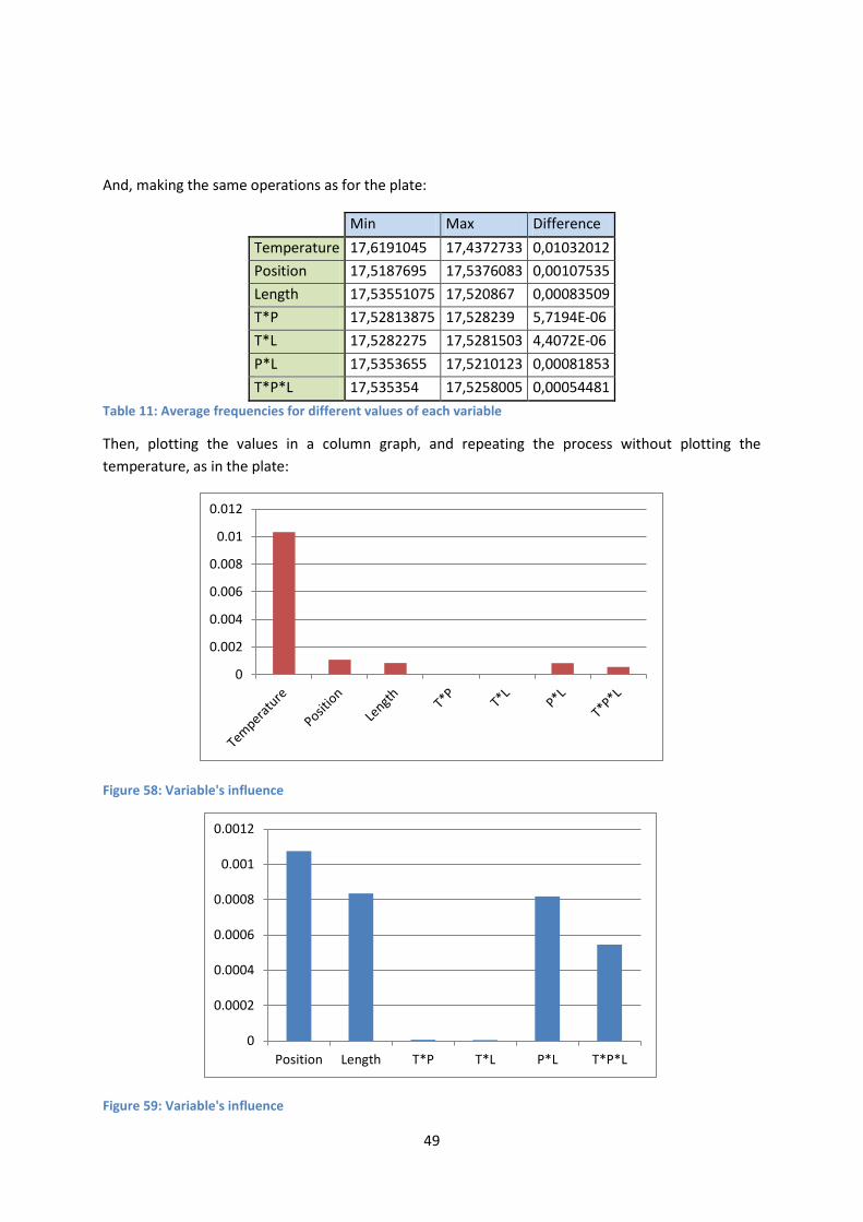
49

And, making the same operations as for the plate:

Min Max Difference

Temperature 17,6191045 17,4372733 0,01032012

Position 17,5187695 17,5376083 0,00107535

Length 17,53551075 17,520867 0,00083509

T*P 17,52813875 17,528239 5,7194E-06

T*L 17,5282275 17,5281503 4,4072E-06

P*L 17,5353655 17,5210123 0,00081853

T*P*L 17,535354 17,5258005 0,00054481

Table 11: Average frequencies for different values of each variable

Then, plotting the values in a column graph, and repeating the process without plotting the

temperature, as in the plate:



0

0.002

0.004

0.006

0.008

0.01

0.012

0

0.0002

0.0004

0.0006

0.0008

0.001

0.0012

Position Length T*P T*L P*L T*P*L

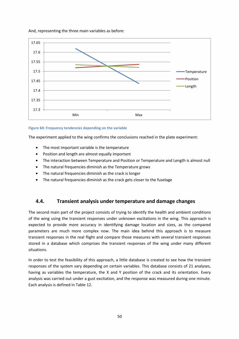
50

And, representing the three main variables as before:

Figure 60: Frequency tendencies depending on the variable

The experiment applied to the wing confirms the conclusions reached in the plate experiment:

The most important variable is the temperature

Position and length are almost equally important

The interaction between Temperature and Position or Temperature and Length is almost null

The natural frequencies diminish as the Temperature grows

The natural frequencies diminish as the crack is longer

The natural frequencies diminish as the crack gets closer to the fuselage

4.4. Transient analysis under temperature and damage changes

The second main part of the project consists of trying to identify the health and ambient conditions

of the wing using the transient responses under unknown excitations in the wing. This approach is

expected to provide more accuracy in identifying damage location and sizes, as the compared

parameters are much more complex now. The main idea behind this approach is to measure

transient responses in the real flight and compare those measures with several transient responses

stored in a database which comprises the transient responses of the wing under many different

situations.

In order to test the feasibility of this approach, a little database is created to see how the transient

responses of the system vary depending on certain variables. This database consists of 21 analyses,

having as variables the temperature, the X and Y position of the crack and its orientation. Every

analysis was carried out under a gust excitation, and the response was measured during one minute.

Each analysis is defined in Table 12.

17.3

17.35

17.4

17.45

17.5

17.55

17.6

17.65

Min Max

Temperature

Position

Length

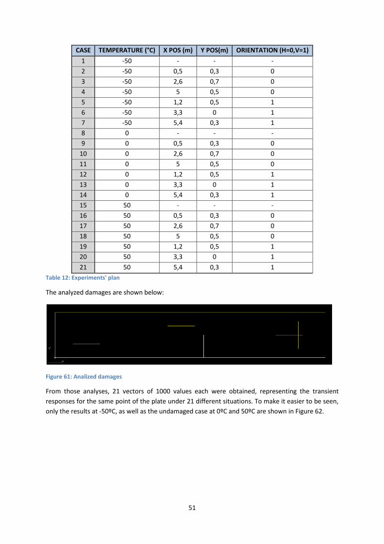
51

CASE TEMPERATURE (°C) X POS (m) Y POS(m) ORIENTATION (H=0,V=1)

1 -50 - - -

2 -50 0,5 0,3 0

3 -50 2,6 0,7 0

4 -50 5 0,5 0

5 -50 1,2 0,5 1

6 -50 3,3 0 1

7 -50 5,4 0,3 1

8 0 - - -

9 0 0,5 0,3 0

10 0 2,6 0,7 0

11 0 5 0,5 0

12 0 1,2 0,5 1

13 0 3,3 0 1

14 0 5,4 0,3 1

15 50 - - -

16 50 0,5 0,3 0

17 50 2,6 0,7 0

18 50 5 0,5 0

19 50 1,2 0,5 1

20 50 3,3 0 1

21 50 5,4 0,3 1

Table 12: Experiments' plan

The analyzed damages are shown below:

Figure 61: Analized damages

From those analyses, 21 vectors of 1000 values each were obtained, representing the transient

responses for the same point of the plate under 21 different situations. To make it easier to be seen,

only the results at -50ºC, as well as the undamaged case at 0ºC and 50ºC are shown in Figure 62.

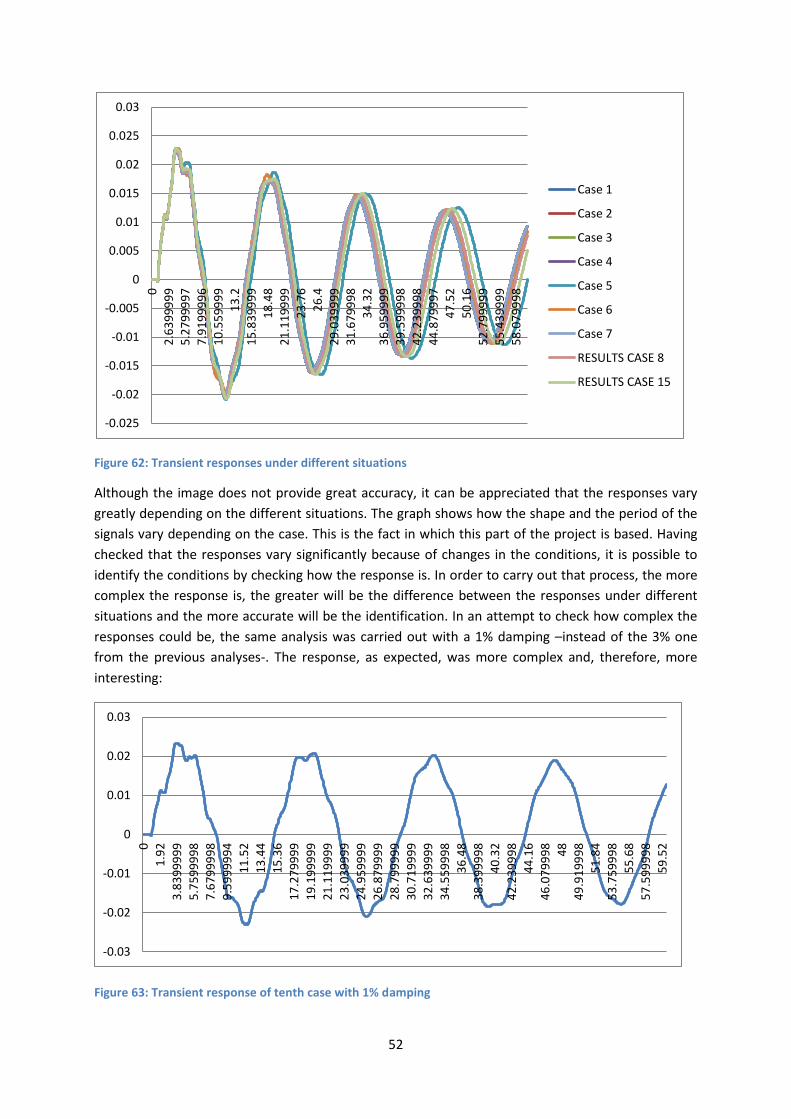
52

Figure 62: Transient responses under different situations

Although the image does not provide great accuracy, it can be appreciated that the responses vary

greatly depending on the different situations. The graph shows how the shape and the period of the

signals vary depending on the case. This is the fact in which this part of the project is based. Having

checked that the responses vary significantly because of changes in the conditions, it is possible to

identify the conditions by checking how the response is. In order to carry out that process, the more

complex the response is, the greater will be the difference between the responses under different

situations and the more accurate will be the identification. In an attempt to check how complex the

responses could be, the same analysis was carried out with a 1% damping –instead of the 3% one

from the previous analyses-. The response, as expected, was more complex and, therefore, more

interesting:

Figure 63: Transient response of tenth case with 1% damping

-0.025

-0.02

-0.015

-0.01

-0.005

0

0.005

0.01

0.015

0.02

0.025

0.03

02

.63

99

99

95

.27

99

99

77

.91

99

99

61

0.5

59

99

91

3.2

15

.83

99

99

18

.48

21

.11

99

99

23

.76

26

.4

29

.03

99

99

31

.67

99

98

34

.32

36

.95

99

99

39

.59

99

98

42

.23

99

98

44

.87

99

97

47

.52

50

.16

52

.79

99

99

55

.43

99

99

58

.07

99

98

Case 1

Case 2

Case 3

Case 4

Case 5

Case 6

Case 7

RESULTS CASE 8

RESULTS CASE 15

-0.03

-0.02

-0.01

0

0.01

0.02

0.03

0

1.9

2

3.8

39

99

99

5.7

59

99

98

7.6

79

99

98

9.5

99

99

94

11

.52

13

.44

15

.36

17

.27

99

99

19

.19

99

99

21

.11

99

99

23

.03

99

99

24

.95

99

99

26

.87

99

99

28

.79

99

99

30

.71

99

99

32

.63

99

99

34

.55

99

98

36

.48

38

.39

99

98

40

.32

42

.23

99

98

44

.16

46

.07

99

98

48

49

.91

99

98

51

.84

53

.75

99

98

55

.68

57

.59

99

98

59

.52

53

In this part it has been demonstrated that the transient responses vary depending on the situation;

however, it is not easy to establish a rule or a mathematic formula able to determine the conditions

when having a transient response signal as an input. That is where the database approach comes. It

aims to compare the real signal with the simulated ones, and see which one is closer, giving

approximately the conditions, all of this without directly linking the shape or the period to the

conditions and, actually, without investigating the relationship.

4.5. Transient analyses under complex turbulence scenario

When it comes to create a database of transient responses it is not feasible to carry out the analysis

under very complex excitations. This is because it would add too many new variables to the

database, making it unaffordable. For this reason, the excitation in the final database is defined just

by one parameter, which is the bandwidth, and the other parameters are constant. However, in

order to see how the responses could be, a complex scenario of excitations is created. It is necessary

because the previous part of the project creates a complex scenario of damage and temperature, but

not regarding the excitations –not necessary to extract the natural frequencies-, which remain simple

and constant for each analysis. Including complex excitations would have meant needing too many

analyses to test many possible combinations of variables. For this reason, a complex scenario of

damage and temperature and a complex scenario of excitations are studied separately. The main

difference between this and the previous analyses is to create random excitations to apply to the

Plate and the Wing, for this reason it will be explained in detail how to do it.

a. Excitement creation

An excel file has been created in order to generate random gust signals, with different amplitude,

different length, and applied at different time. The forces which will follow those fields are also

defined, choosing randomly the point in which they are applied and their direction. The amplitude is

defined by a random number between 0 and 1 multiplied by the maximum desirable amplitude. The

direction is defined by its three components, being each one a random number between 0 and 1. To

choose the location of the signal in time, the middle point of the signal is chosen by choosing a real

number from 0 to the total length of the time. Then, as the half of the total length of the signal has to

be shorter than the shortest part of the 2 parts divided by the middle point, the minimum is chosen,

and then, a random number from the middle point to the end of the shortest part is chosen

randomly, being the end or the beginning of the signal. For example, if the total length is 30 second,

a real number is chosen randomly. Imagine that the number is 17.2. Then, the middle of the gust will

be located there, and the total length of the period will be divided into two parts, the first one of

17.2 seconds and the other one of 12.8. The minimum of both is 12.8; therefore, a real number

between 0 and 12.8 will be chosen. Imagine that this number is 9.6, then, the beginning of the gust

will be located at 17.2-9.6=7.6 seconds and the end at 17.2+9.6=26.8 seconds.

To introduce this signals in Patran as a field some steps must be followed. First of all, the two

columns (time and value) that define a signal have to be copied into a new excel file. This file must be

saved as a .csv (semi-colon separator). Then it has to be renamed as .txt and opened. In the Notepad,

the tool “Replace” (In Edition menu) will be used to change all the “,” by “.”, because that is the way

in which Patran works. Then the file must be saved and renamed again as .csv. Once opened Patran,

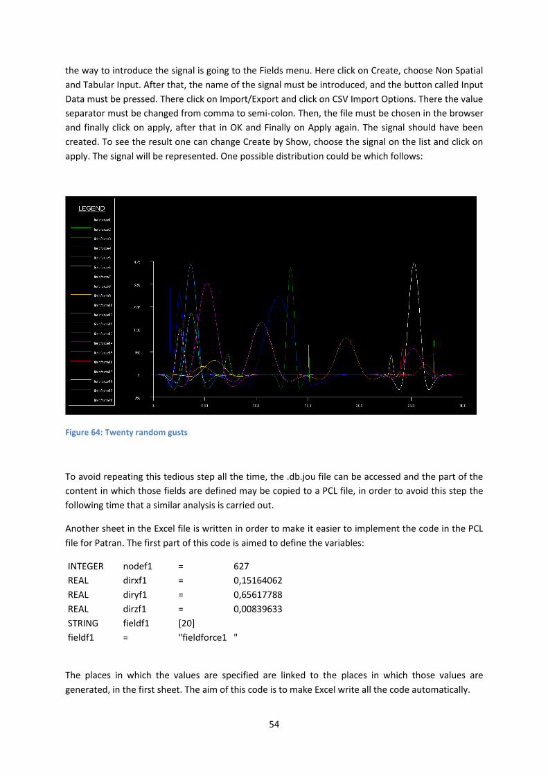
54

the way to introduce the signal is going to the Fields menu. Here click on Create, choose Non Spatial

and Tabular Input. After that, the name of the signal must be introduced, and the button called Input

Data must be pressed. There click on Import/Export and click on CSV Import Options. There the value

separator must be changed from comma to semi-colon. Then, the file must be chosen in the browser

and finally click on apply, after that in OK and Finally on Apply again. The signal should have been

created. To see the result one can change Create by Show, choose the signal on the list and click on

apply. The signal will be represented. One possible distribution could be which follows:

Figure 64: Twenty random gusts

To avoid repeating this tedious step all the time, the .db.jou file can be accessed and the part of the

content in which those fields are defined may be copied to a PCL file, in order to avoid this step the

following time that a similar analysis is carried out.

Another sheet in the Excel file is written in order to make it easier to implement the code in the PCL

file for Patran. The first part of this code is aimed to define the variables:

INTEGER nodef1 = 627

REAL dirxf1 = 0,15164062

REAL diryf1 = 0,65617788

REAL dirzf1 = 0,00839633

STRING fieldf1 [20]

fieldf1 = "fieldforce1 "

The places in which the values are specified are linked to the places in which those values are

generated, in the first sheet. The aim of this code is to make Excel write all the code automatically.

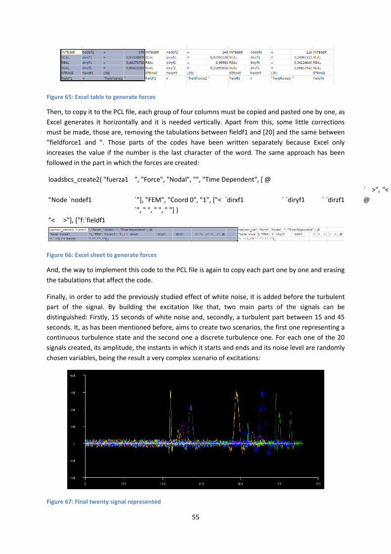
55

Figure 65: Excel table to generate forces

Then, to copy it to the PCL file, each group of four columns must be copied and pasted one by one, as

Excel generates it horizontally and it is needed vertically. Apart from this, some little corrections

must be made, those are, removing the tabulations between fieldf1 and [20] and the same between

“fieldforce1 and “. Those parts of the codes have been written separately because Excel only

increases the value if the number is the last character of the word. The same approach has been

followed in the part in which the forces are created:

loadsbcs_create2( "fuerza1 ", "Force", "Nodal", "", "Time Dependent", [ @

"Node `nodef1 `"], "FEM", "Coord 0", "1", ["< `dirxf1 ` `diryf1 ` `dirzf1

` >", "< >", "< >",

@

"< >"], ["f:`fieldf1

`", " ", " ", " "] )

Figure 66: Excel sheet to generate forces

And, the way to implement this code to the PCL file is again to copy each part one by one and erasing

the tabulations that affect the code.

Finally, in order to add the previously studied effect of white noise, it is added before the turbulent

part of the signal. By building the excitation like that, two main parts of the signals can be

distinguished: Firstly, 15 seconds of white noise and, secondly, a turbulent part between 15 and 45

seconds. It, as has been mentioned before, aims to create two scenarios, the first one representing a

continuous turbulence state and the second one a discrete turbulence one. For each one of the 20

signals created, its amplitude, the instants in which it starts and ends and its noise level are randomly

chosen variables, being the result a very complex scenario of excitations:

Figure 67: Final twenty signal represented

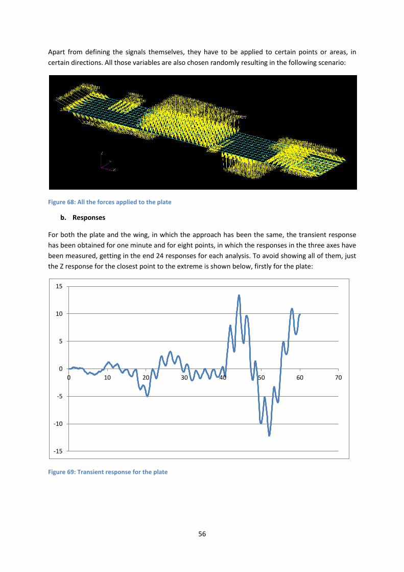
56

Apart from defining the signals themselves, they have to be applied to certain points or areas, in

certain directions. All those variables are also chosen randomly resulting in the following scenario:

Figure 68: All the forces applied to the plate

b. Responses

For both the plate and the wing, in which the approach has been the same, the transient response

has been obtained for one minute and for eight points, in which the responses in the three axes have

been measured, getting in the end 24 responses for each analysis. To avoid showing all of them, just

the Z response for the closest point to the extreme is shown below, firstly for the plate:

Figure 69: Transient response for the plate

-15

-10

-5

0

5

10

15

0 10 20 30 40 50 60 70

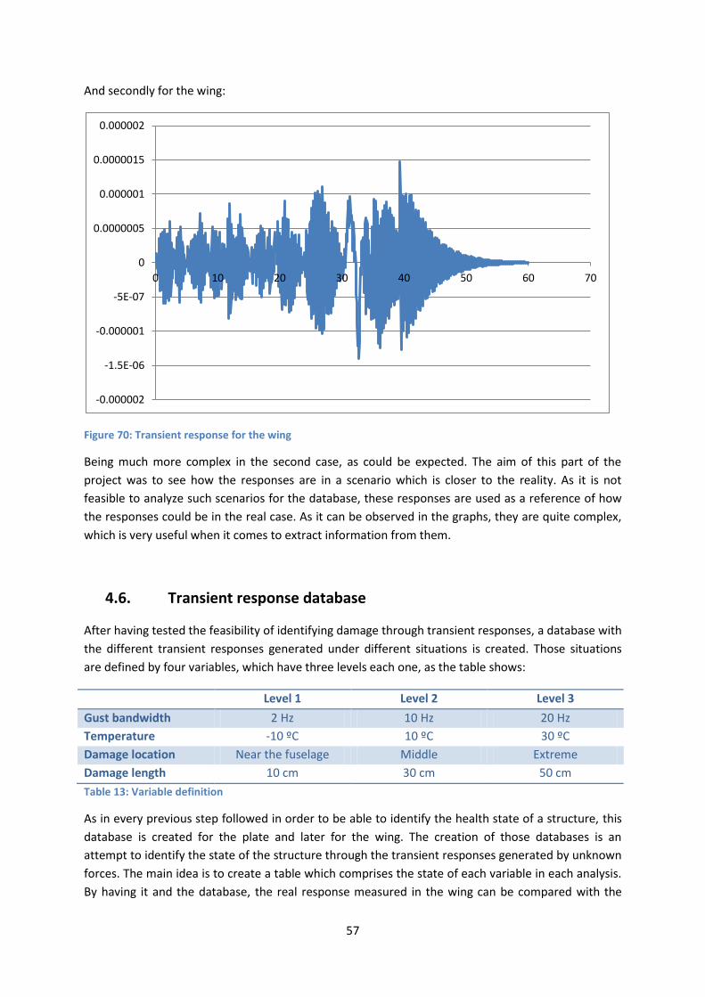
57

And secondly for the wing:

Figure 70: Transient response for the wing

Being much more complex in the second case, as could be expected. The aim of this part of the

project was to see how the responses are in a scenario which is closer to the reality. As it is not

feasible to analyze such scenarios for the database, these responses are used as a reference of how

the responses could be in the real case. As it can be observed in the graphs, they are quite complex,

which is very useful when it comes to extract information from them.

4.6. Transient response database

After having tested the feasibility of identifying damage through transient responses, a database with

the different transient responses generated under different situations is created. Those situations

are defined by four variables, which have three levels each one, as the table shows:

Level 1 Level 2 Level 3

Gust bandwidth 2 Hz 10 Hz 20 Hz

Temperature -10 ºC 10 ºC 30 ºC

Damage location Near the fuselage Middle Extreme

Damage length 10 cm 30 cm 50 cm

Table 13: Variable definition

As in every previous step followed in order to be able to identify the health state of a structure, this

database is created for the plate and later for the wing. The creation of those databases is an

attempt to identify the state of the structure through the transient responses generated by unknown

forces. The main idea is to create a table which comprises the state of each variable in each analysis.

By having it and the database, the real response measured in the wing can be compared with the

-0.000002

-1.5E-06

-0.000001

-5E-07

0

0.0000005

0.000001

0.0000015

0.000002

0 10 20 30 40 50 60 70

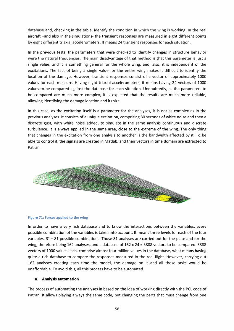
58

database and, checking in the table, identify the condition in which the wing is working. In the real

aircraft –and also in the simulations- the transient responses are measured in eight different points

by eight different triaxial accelerometers. It means 24 transient responses for each situation.

In the previous tests, the parameters that were checked to identify changes in structure behavior

were the natural frequencies. The main disadvantage of that method is that this parameter is just a

single value, and it is something general for the whole wing, and, also, it is independent of the

excitations. The fact of being a single value for the entire wing makes it difficult to identify the

location of the damage. However, transient responses consist of a vector of approximately 1000

values for each measure. Having eight triaxial accelerometers, it means having 24 vectors of 1000

values to be compared against the database for each situation. Undoubtedly, as the parameters to

be compared are much more complex, it is expected that the results are much more reliable,

allowing identifying the damage location and its size.

In this case, as the excitation itself is a parameter for the analyses, it is not as complex as in the

previous analyses. It consists of a unique excitation, comprising 30 seconds of white noise and then a

discrete gust, with white noise added, to simulate in the same analysis continuous and discrete

turbulence. It is always applied in the same area, close to the extreme of the wing. The only thing

that changes in the excitation from one analysis to another is the bandwidth affected by it. To be

able to control it, the signals are created in Matlab, and their vectors in time domain are extracted to

Patran.

Figure 71: Forces applied to the wing

In order to have a very rich database and to know the interactions between the variables, every

possible combination of the variables is taken into account. It means three levels for each of the four

variables, 3⁴ = 81 possible combinations. Those 81 analyses are carried out for the plate and for the

wing, therefore being 162 analyses, and a database of 162 x 24 = 3888 vectors to be compared. 3888

vectors of 1000 values each, comprise almost four million values in the database, what means having

quite a rich database to compare the responses measured in the real flight. However, carrying out

162 analyses creating each time the model, the damage on it and all those tasks would be

unaffordable. To avoid this, all this process have to be automated.

a. Analysis automation

The process of automating the analyses in based on the idea of working directly with the PCL code of

Patran. It allows playing always the same code, but changing the parts that must change from one

59

analysis to another. As the code may result very long and some of the things that must be changed

may appear several times, the best approach is to define those features as variables at the beginning,

making it easier to change them and replay the code. Fully automating the analysis means that, once

the values of every variable have been set, the PCL code is run and it carries out all the process, and

the user must not interact with Patran’s interface.

Firstly, a name must be assigned to the job. As this name appears in various parts of de code, it will

be represented by a variable as follows:

STRING jobnom[20]

jobnom = “first_job”

The way to create the boundary conditions, the forces, the materials, the properties and everything

which is necessary to define the problem is supposed to be known, therefore, how to automate the

analysis will be directly presented. In this case it will consist of a transient analysis, with modal

damping set by a variable (Critical damping chosen). The time steps chosen are 1000 steps of 0.06

seconds each. The way to automate it is to carry it out manually and step by step copy the code that

the program generates while the analysis is being defined from the .db.jou file to the written code.

By doing so, the following code allows carrying out the analysis automatically, represents the

transient response and save its 1000 values in a .xyd file, named as the user wishes where the user

wishes. The name of this file will be defined by a variable:

STRING nomgraf[20]

nomgraf = "filename"

REAL temper = 20

REAL damping = 0.01

INTEGER nodegraf = 364

The variables called temper and damping represent the temperature and the damping coefficient,

respectively. Nodegraf represents the point in which the transient response is represented and its

values saved.

In order to obtain the transient response of a point and save its values on a file, the process followed

in Patran has been:

Clicking on “Analysis” button

Select Analyze, Entire model, Full run

Enter a job name (in the code it will be replaced by a variable)

Click on Solution Type and select Transient Response

Click on Solution parameters and there define the temperature in “default initial

temperature” field (will be replaced by a variable) and click on Ok and Ok again

Click on subcases, choose the one which will be used and click on subcase parameters

Define the time steps and the damping (later it will be replaced by a variable)

Ok, Apply and select this subcase in “subcases select”

Click on apply to carry out the analysis

Once the analysis has been finished, the process to obtain the curve is:

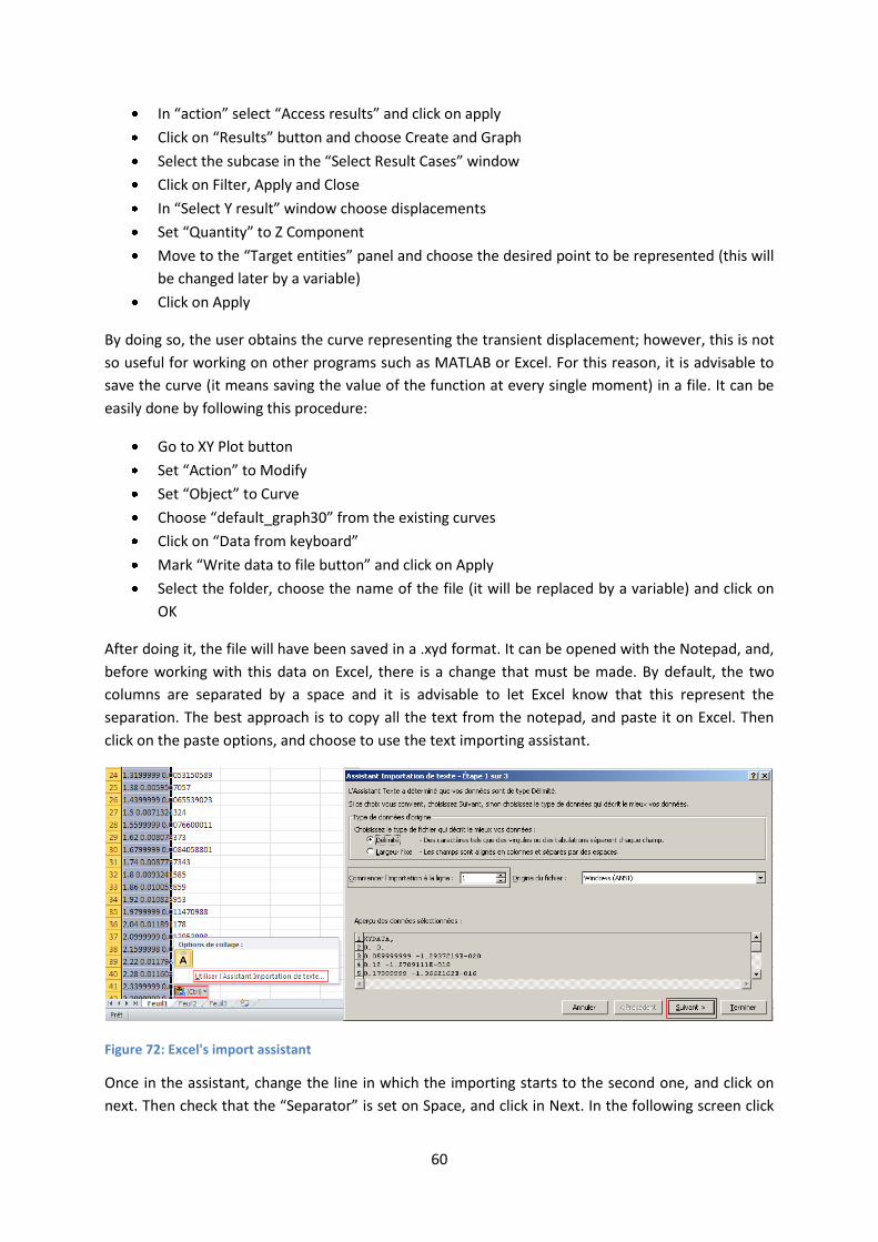
60

In “action” select “Access results” and click on apply

Click on “Results” button and choose Create and Graph

Select the subcase in the “Select Result Cases” window

Click on Filter, Apply and Close

In “Select Y result” window choose displacements

Set “Quantity” to Z Component

Move to the “Target entities” panel and choose the desired point to be represented (this will

be changed later by a variable)

Click on Apply

By doing so, the user obtains the curve representing the transient displacement; however, this is not

so useful for working on other programs such as MATLAB or Excel. For this reason, it is advisable to

save the curve (it means saving the value of the function at every single moment) in a file. It can be

easily done by following this procedure:

Go to XY Plot button

Set “Action” to Modify

Set “Object” to Curve

Choose “default_graph30” from the existing curves

Click on “Data from keyboard”

Mark “Write data to file button” and click on Apply

Select the folder, choose the name of the file (it will be replaced by a variable) and click on

OK

After doing it, the file will have been saved in a .xyd format. It can be opened with the Notepad, and,

before working with this data on Excel, there is a change that must be made. By default, the two

columns are separated by a space and it is advisable to let Excel know that this represent the

separation. The best approach is to copy all the text from the notepad, and paste it on Excel. Then

click on the paste options, and choose to use the text importing assistant.

Figure 72: Excel's import assistant

Once in the assistant, change the line in which the importing starts to the second one, and click on

next. Then check that the “Separator” is set on Space, and click in Next. In the following screen click

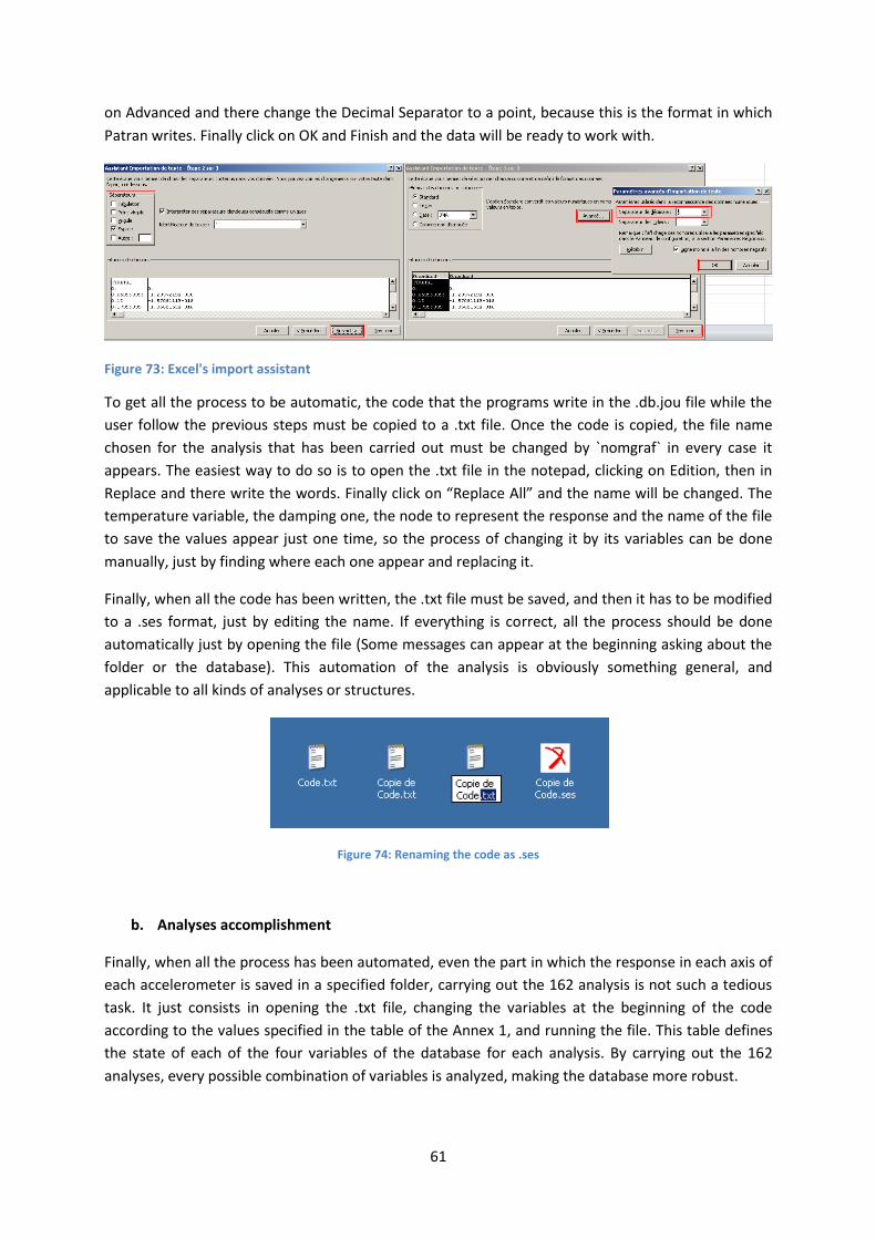
61

on Advanced and there change the Decimal Separator to a point, because this is the format in which

Patran writes. Finally click on OK and Finish and the data will be ready to work with.

Figure 73: Excel's import assistant

To get all the process to be automatic, the code that the programs write in the .db.jou file while the

user follow the previous steps must be copied to a .txt file. Once the code is copied, the file name

chosen for the analysis that has been carried out must be changed by `nomgraf` in every case it

appears. The easiest way to do so is to open the .txt file in the notepad, clicking on Edition, then in

Replace and there write the words. Finally click on “Replace All” and the name will be changed. The

temperature variable, the damping one, the node to represent the response and the name of the file

to save the values appear just one time, so the process of changing it by its variables can be done

manually, just by finding where each one appear and replacing it.

Finally, when all the code has been written, the .txt file must be saved, and then it has to be modified

to a .ses format, just by editing the name. If everything is correct, all the process should be done

automatically just by opening the file (Some messages can appear at the beginning asking about the

folder or the database). This automation of the analysis is obviously something general, and

applicable to all kinds of analyses or structures.

Figure 74: Renaming the code as .ses

b. Analyses accomplishment

Finally, when all the process has been automated, even the part in which the response in each axis of

each accelerometer is saved in a specified folder, carrying out the 162 analysis is not such a tedious

task. It just consists in opening the .txt file, changing the variables at the beginning of the code

according to the values specified in the table of the Annex 1, and running the file. This table defines

the state of each of the four variables of the database for each analysis. By carrying out the 162

analyses, every possible combination of variables is analyzed, making the database more robust.

62

Storing so much information (162x24=3888 responses) is not a problem nowadays; however, as the

aim of this project is to allow identifying the aircraft health state while it is working, it is advisable

that the identification does not take too much time, to be able to monitor the state of the structure

almost in real time. To reduce the time spent in the comparisons between signals, the signals can be

compressed, extracting the most of the information from them in the least possible data. Since it

goes beyond the scope of the project, it is further explained in “Results and comments” chapter. It is

also explained there what to do with the created database, as the aim of the project is just to create

it, without using it to perform the modal identification.

63

5. Results and comments

As a research project, the expected results are not actual data, but different conclusions about

different approaches to carry out Structural Health Monitoring. Furthermore, the end of this project

aims to be the beginning of another one, as it set the basis for future studies in the field.

First of all, it has been checked that temperature changes and damage affects the natural

frequencies in a different way, which can be very useful to separate the contribution of each one to

the measured change in natural frequencies. The contribution of a temperature change is very easy

to identify, as it changes every natural frequency in the same proportions. As the ambient

temperature is something easy to know, its effect can be calculated and suppressed from the

changes that the natural frequencies have suffered. Then, the main changes in them would be due to

damage; however, natural frequencies are not very good estimators to identify the size and location

of damage, therefore making necessary other approach, that must not be substitutive of the natural

frequencies one, but complementary. Another conclusion extracted from the analyses is that the

change in the natural frequencies is much greater due to the effect of temperature than because of

damage. Also, a little approximation to the size and location of the damage can be made with the

natural frequencies, since some tendencies have been noticed in them depending on those

parameters (Point 4.3). Other possible approach to be followed in order to guess where the damage

is through the natural frequencies changes is to take into account that they are affected greatly or

slightly depending on the position of the crack with regard to the mode shapes and the nodes of the

shape (Point 4.2.d). By checking which modes are more affected and analyzing their shapes, a first

guess can be made regarding the damage location. As all these approaches are based on the natural

frequency shifts, it is essential to be able to obtain them during the flight. To be able to perform such

a task, it has been analyzed whether the discrete and continuous turbulences can be used or not

(Point 4.1). The experiment shows that they can be obtained easily, with a very acceptable accuracy

following the shown procedure, therefore being a good option to obtain the natural frequencies,

necessary to identify the state of the structure as has been mentioned before.

The other option, complementary to the previous one, consists of using a database of transient

responses to make the identification. It has been noticed that they change sufficiently due to damage

and temperature effect to be used as parameters (Point 4.4) and, actually, are much more complex

and comprise more data than the natural frequencies, making more accurate the location of the

damage and the guess of its size. In fact, the real transient responses would be much more complex,

as the excitation would be more complex (Point 4.5) making it even better the identification.

Regarding this kind of identification, it is a must to go deeper in separating the effect of temperature

and damage, being a possibility to use the natural frequencies to do such a task, as temperature

effect is easy to separate in them. Apart from this, it is not easy to identify a pattern in the transient

responses which allow easily identifying damage size and locations. Therefore, the chosen way to do

it is to create a database and compare the real responses with those stored in the database. Also,

different orientations should be studied for the cracks, as the created database only represents the

effect of horizontal damage.

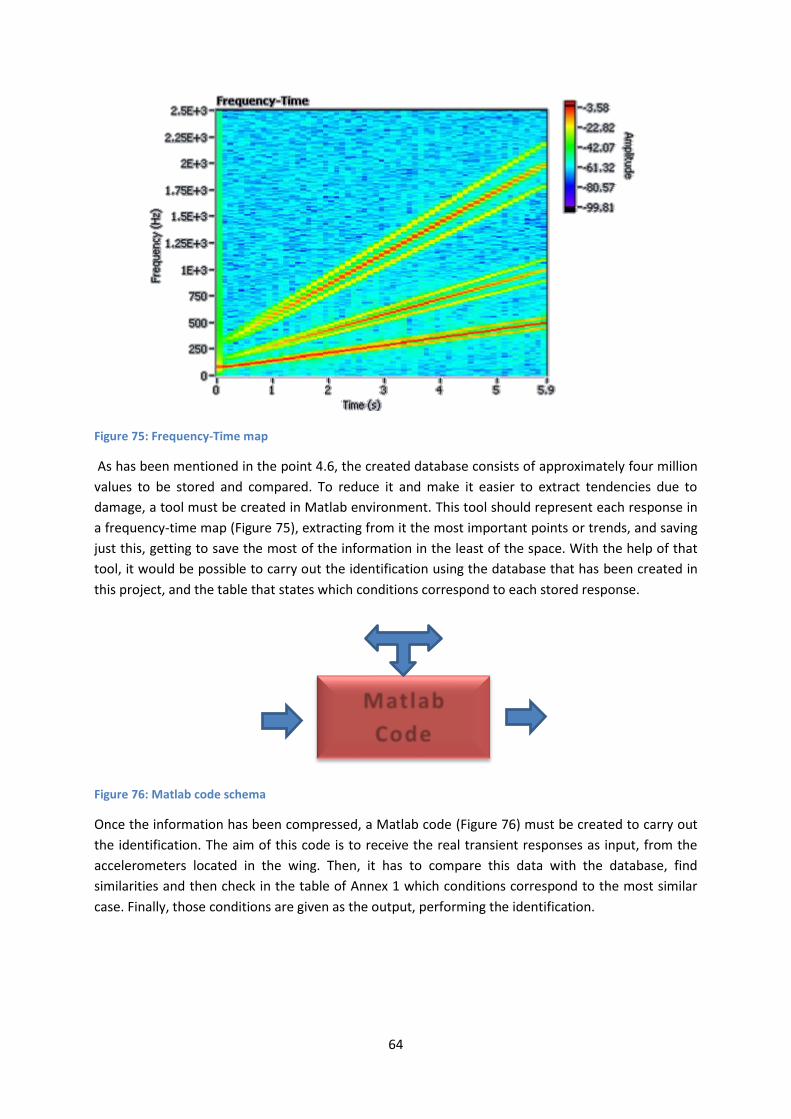
64

Figure 75: Frequency-Time map

As has been mentioned in the point 4.6, the created database consists of approximately four million

values to be stored and compared. To reduce it and make it easier to extract tendencies due to

damage, a tool must be created in Matlab environment. This tool should represent each response in

a frequency-time map (Figure 75), extracting from it the most important points or trends, and saving

just this, getting to save the most of the information in the least of the space. With the help of that

tool, it would be possible to carry out the identification using the database that has been created in

this project, and the table that states which conditions correspond to each stored response.

Figure 76: Matlab code schema

Once the information has been compressed, a Matlab code (Figure 76) must be created to carry out

the identification. The aim of this code is to receive the real transient responses as input, from the

accelerometers located in the wing. Then, it has to compare this data with the database, find

similarities and then check in the table of Annex 1 which conditions correspond to the most similar

case. Finally, those conditions are given as the output, performing the identification.

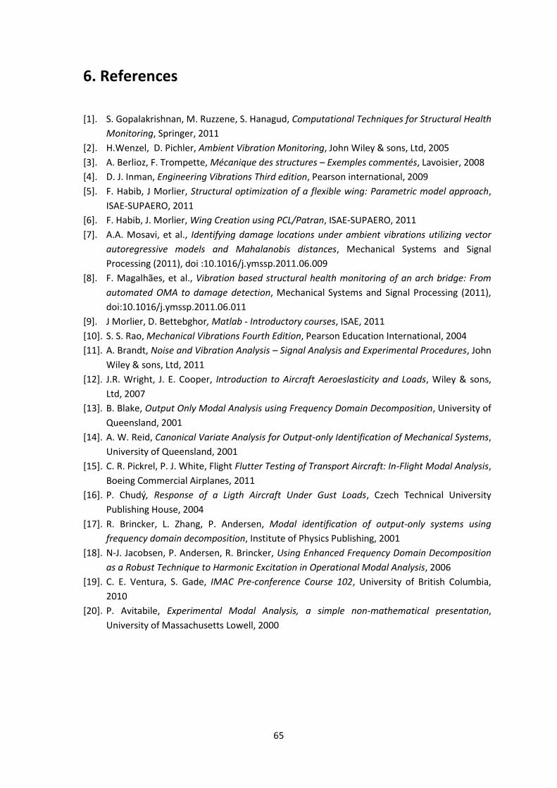
65

6. References

[1]. S. Gopalakrishnan, M. Ruzzene, S. Hanagud, Computational Techniques for Structural Health

Monitoring, Springer, 2011

[2]. H.Wenzel, D. Pichler, Ambient Vibration Monitoring, John Wiley & sons, Ltd, 2005

[3]. A. Berlioz, F. Trompette, Mécanique des structures – Exemples commentés, Lavoisier, 2008

[4]. D. J. Inman, Engineering Vibrations Third edition, Pearson international, 2009

[5]. F. Habib, J Morlier, Structural optimization of a flexible wing: Parametric model approach,

ISAE-SUPAERO, 2011

[6]. F. Habib, J. Morlier, Wing Creation using PCL/Patran, ISAE-SUPAERO, 2011

[7]. A.A. Mosavi, et al., Identifying damage locations under ambient vibrations utilizing vector

autoregressive models and Mahalanobis distances, Mechanical Systems and Signal

Processing (2011), doi :10.1016/j.ymssp.2011.06.009

[8]. F. Magalhães, et al., Vibration based structural health monitoring of an arch bridge: From

automated OMA to damage detection, Mechanical Systems and Signal Processing (2011),

doi:10.1016/j.ymssp.2011.06.011

[9]. J Morlier, D. Bettebghor, Matlab - Introductory courses, ISAE, 2011

[10]. S. S. Rao, Mechanical Vibrations Fourth Edition, Pearson Education International, 2004

[11]. A. Brandt, Noise and Vibration Analysis – Signal Analysis and Experimental Procedures, John

Wiley & sons, Ltd, 2011

[12]. J.R. Wright, J. E. Cooper, Introduction to Aircraft Aeroeslasticity and Loads, Wiley & sons,

Ltd, 2007

[13]. B. Blake, Output Only Modal Analysis using Frequency Domain Decomposition, University of

Queensland, 2001

[14]. A. W. Reid, Canonical Variate Analysis for Output-only Identification of Mechanical Systems,

University of Queensland, 2001

[15]. C. R. Pickrel, P. J. White, Flight Flutter Testing of Transport Aircraft: In-Flight Modal Analysis,

Boeing Commercial Airplanes, 2011

[16]. P. Chudý, Response of a Ligth Aircraft Under Gust Loads, Czech Technical University

Publishing House, 2004

[17]. R. Brincker, L. Zhang, P. Andersen, Modal identification of output-only systems using

frequency domain decomposition, Institute of Physics Publishing, 2001

[18]. N-J. Jacobsen, P. Andersen, R. Brincker, Using Enhanced Frequency Domain Decomposition

as a Robust Technique to Harmonic Excitation in Operational Modal Analysis, 2006

[19]. C. E. Ventura, S. Gade, IMAC Pre-conference Course 102, University of British Columbia,

2010

[20]. P. Avitabile, Experimental Modal Analysis, a simple non-mathematical presentation,

University of Massachusetts Lowell, 2000

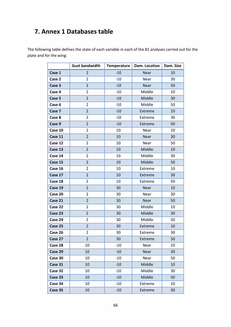
66

7. Annex 1 Databases table

The following table defines the state of each variable in each of the 81 analyses carried out for the

plate and for the wing:

Gust bandwidth Temperature Dam. Location Dam. Size

Case 1 2 -10 Near 10



Case 4 2 -10 Middle 10



Case 7 2 -10 Extreme 10



Case 10 2 10 Near 10



Case 13 2 10 Middle 10



Case 16 2 10 Extreme 10












Case 28 10 -10 Near 10

Case 29 10 -10 Near 30

Case 30 10 -10 Near 50






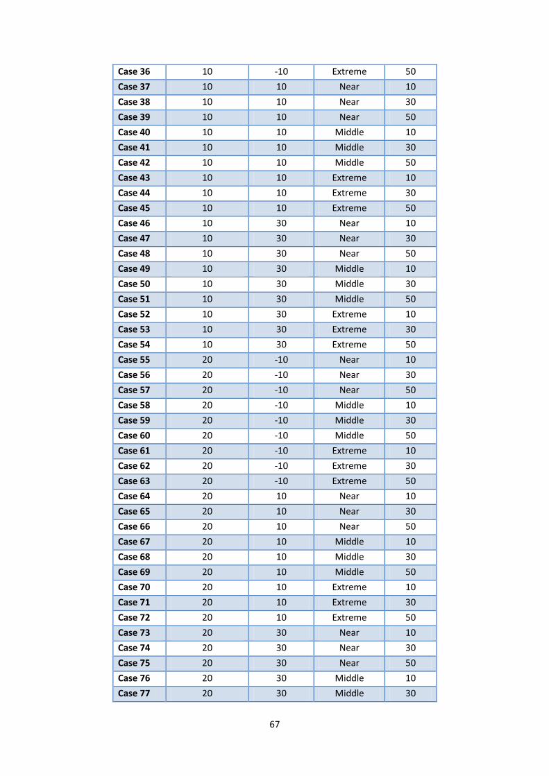
67


Case 37 10 10 Near 10

Case 38 10 10 Near 30

Case 39 10 10 Near 50







Case 46 10 30 Near 10

Case 47 10 30 Near 30

Case 48 10 30 Near 50







Case 55 20 -10 Near 10

Case 56 20 -10 Near 30

Case 57 20 -10 Near 50







Case 64 20 10 Near 10

Case 65 20 10 Near 30

Case 66 20 10 Near 50







Case 73 20 30 Near 10

Case 74 20 30 Near 30

Case 75 20 30 Near 50



68





Table 14: Experiments plan

69

8. Annex 2: Software

8.1. Patran/Nastran

Since MSC Nastran is the most widely used Finite Element Analysis (FEA) software in the world, it is

the program in which this project has been based, becoming a fundamental part of it, as every

analysis carried out has been performed by Nastran. More accurately, the software version used has

been the 2010.1, and Patran software has been used as the interface for the pre and post-processing

parts. Its versatility allows creating many different types of structures, allowing the user creating

different geometries, meshing, materials, forces and defining different kind of analysis to be carried

out by Nastran. Once Nastran’s work has been finished, Patran will present the results of the analysis

and will show the deformation, stresses and whatever is demanded.

In order to be able to do so, a very time-consuming part of the project consists of learning the

necessary software, including Patran. Regarding this FEA software, the objectives to be achieved

when learning the program were:

Build models of simple or middle complexity

Learn how to carry out Modal Analysis

Learn how to carry out Transient Analysis

Obtain Frequency Response Functions (FRF)

Simulate damage in a structure

Implementation of signals from Matlab and Excel

Results extracting

Parametric programming in PCL

Simulate changes in temperature

The way to learn them has been to follow some tutorials written both by MSC Software, which is the

company behind Nastran and Patran, and previous students doing an internship at SUPAERO. A list of

those tutorials is provided below, sorted in chronological order:

Initiation à Patran pour des calcul des structures

Simple Stress Analysis of a solid

Beam Static Analysis

Read/edit a bdf file

Direct Transient Analysis

Modal Transient Analysis

Modal Frequency Response Analysis

Normal Modes Analysis

Etude dynamique d’une plaque impactée

Global/Local Modeling using FEM fields

Creating PCL Functions

PCL via session file

Wing Creation using PCL/Patran

70

Regarding the objectives and, taking into account the nature of the project, probably the most

important one might be the ability to carry out transient analysis. In order to go deeper in this

aspect, an online lecture on that topic was followed from the United States, lectured by an expert

worker of MSC Software. It provided complementary information about those analyses and different

approaches which had not been explained in the tutorials.

Finally, the last, but not least important, way of learning has been the self-learning. By spending such

an amount of hours using this software, many different actions are learnt by searching new tools in

the menus, looking for solutions on the Internet, etc. Apart from this, as usual in science, the trial and

error approach has helped very much to learn about the program and how to use it.

8.2. Matlab

Although the project is based on Patran/Nastran, it is also necessary to generate previously all the

things that Patran needs to carry out the analyses and to be able to manage the results it generates.

All of those tasks must be carried out in a different environment, such as Matlab. Matlab is a

software program which works with matrixes, allowing doing whatever is needed with them. In this

case, the aims in using Matlab have been:

Create signals to be implemented as excitations in Patran/Nastran

Obtain Spectral Density Functions

Results processing

Structural Identification

As in the case of Patran, the way to learn to use this software was initially based on following

tutorials, however, once a general idea of how it works has been acquired, the main tool used to

learn new commands or tools was the help tool. This tool is full of commands, extensively explained

and it encloses a great number of examples, making it much easier to learn how each command

works.

8.3. Excel

The role played by Excel has been quite similar to Matlab’s one. It has served also as a way to

generate signals or random values for different variables as a previous step of the Patran/Nastran

analyses. It has also served as a tool to manage the results extracted from those analyses. Apart from

those purposes, Excel also has served as an intermediate tool between Matlab and Patran/Nastran.

As the data generated in Matlab is not directly compatible with Patran and vice versa. Another use of

Excel has been to adapt the data from one format to the other. Added to the latter, the main

objectives pursued when learning Excel have been to:

Adapt Matlab signals to be used in Patran

Generate PCL code

Plot the response vectors

Organize the results and the database

Excel is probably the most widespread software of the three mentioned ones. It means that it was

previously known, preventing the user from needing extra learning on the topic. The experience with

71

the program has been enough in the vast majority of the cases, and, for the rest, self-learning has

been sufficient.

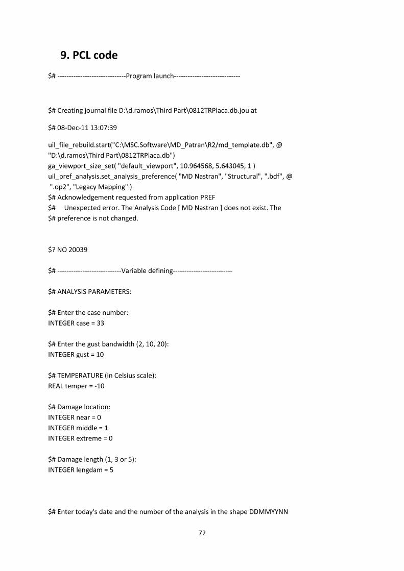
72

9. PCL code

$# ------------------------------Program launch-----------------------------

$# Creating journal file D:\d.ramos\Third Part\0812TRPlaca.db.jou at

$# 08-Dec-11 13:07:39

uil_file_rebuild.start("C:\MSC.Software\MD_Patran\R2/md_template.db", @

"D:\d.ramos\Third Part\0812TRPlaca.db")

ga_viewport_size_set( "default_viewport", 10.964568, 5.643045, 1 )

uil_pref_analysis.set_analysis_preference( "MD Nastran", "Structural", ".bdf", @

".op2", "Legacy Mapping" )

$# Acknowledgement requested from application PREF

$# Unexpected error. The Analysis Code [ MD Nastran ] does not exist. The

$# preference is not changed.

$? NO 20039

$# ----------------------------Variable defining--------------------------

$# ANALYSIS PARAMETERS:

$# Enter the case number:

INTEGER case = 33

$# Enter the gust bandwidth (2, 10, 20):

INTEGER gust = 10

$# TEMPERATURE (in Celsius scale):

REAL temper = -10

$# Damage location:

INTEGER near = 0

INTEGER middle = 1

INTEGER extreme = 0

$# Damage length (1, 3 or 5):

INTEGER lengdam = 5

$# Enter today's date and the number of the analysis in the shape DDMMYYNN

73

STRING date[8]

date = "14011233"

$# Enter a name for the analysis, without spaces (max 10 characters)

STRING name[10]

name = "TRPlate"

$# Enter the folder to save the results (max 70 characters)

STRING folder[70]

folder = "D:\d.ramos\Ninth Part\Plate database\Database\Case 33"

$# Enter the nodes in which the accelerometers are located

INTEGER nodegraf1 = 188








$# GEOMETRY:

REAL lengthx = 6

REAL lengthy = 1

$# MESHING:


$# DAMPING

REAL damping = 0.01

$# FORCES:

INTEGER radius1 = 3

INTEGER nodef1 = 484

REAL dirxf1 = 1

REAL diryf1 = 1

REAL dirzf1 = 1

STRING fieldf1[20]

$# DAMAGE:

74


INTEGER usedam1h = 0





lastelm1h = firstelm1h + `lengdam` + 1

lastnode1h = firstnode1h + `lengdam`

















IF (`near` == 1) THEN

usedam1h = 1

END IF

IF (`middle` == 1) THEN

usedam2h = 1

END IF

IF (èxtreme` == 1) THEN

usedam3h = 1

END IF

IF (`gust` == 2) THEN

fieldf1 = "Gust_2"

END IF


75

fieldf1 = "Gust_10"

END IF


fieldf1 = "Gust_20"

END IF

$# ------------------------------Plate geometry-----------------------------




$# 1 Patch created: Patch 1

$# ---------------------------------Meshing---------------------------------










$# 561 nodes and 500 elements created for Surface 1.

$# === 561 nodes created. IDs = 1:561.

$# === 500 elements created. IDs = 1:500.



mesh_seed_display_mgr.erase( )

$# ----------------------------Boundary conditions---------------------------

loadsbcs_create2( "Fix", "Displacement", "Nodal", "", "Static", ["Surface 1.1" @

], "Geometry", "Coord 0", "1.", ["< 0 0 0 >", "< 0 0 0 >", "< >", @

"< >"], ["", "", "", ""] )

$# Load/BC set "Fix" created.

$# ------------------------------Field E-Temp---------------------------------

fields_create( "E-Temp_Field", "Material", 1, "Scalar", "Real", "", "", @

"Table", 1, "T", "", "", "", "", "", FALSE, [-200., -129., -73., 21., 93., @

149., 204.], [0.], [0.], [[[7.8564278E+010]][[7.6495847E+010]][[7.44274E+010]][[7.0980002E+010]][[

76

@

6.8222079E+010]][[6.546416E+010]][[6.2016762E+010]]] )

$# Field "E-Temp_Field" created.

$# ----------------------------Material Creation------------------------------

material.create( "Analysis code ID", 1, "Analysis type ID", 1, "Material7150", @

0, "Date: 08-Dec-11 Time: 14:30:13", "Isotropic", 1, @

"Directionality", 1, "Linearity", 1, "Homogeneous", 0, "Linear Elastic", 1, @

"Model Options & IDs", ["", "", "", "", ""], [0, 0, 0, 0, 0], "Active Flag", @

1, "Create", 10, "External Flag", FALSE, "Property IDs", ["Elastic Modulus", @

"Poisson Ratio", "Density"], [2, 5, 16, 0], "Property Values", ["E-Temp_Field" @

, "0.3", "2700", ""] )

elementprops_create( "PropiedadesPlaca", 51, 25, 35, 1, 1, 20, [13, 20, 36, @

4037, 4111, 4118, 4119], [5, 9, 1, 1, 1, 1, 1], ["m:Material7150", "", "0.003" @

, "", "", "", ""], "Surface 1" )

$# Property Set "PropiedadesPlaca" created.

uil_toolbar.hidden_line( )

ga_view_aa_set( -67., 0., -34. )

$# ------------------------Signal creation in "Fields"------------------------

fields_create( "Gust 2", "Non-Spatial", 1, "Scalar", "Real", "", "", "Table", @

1, "t", "", "", "", "", "", FALSE, [0., 0.059999999, 0.12, 0.18000001, @

0.23999999, 0.30000001, 0.36000001, 0.41999999, 0.47999999, 0.54000002, @

0.60000002, 0.66000003, 0.72000003, 0.77999997, 0.83999997, 0.89999998, @

0.95999998, 1.02, 1.08, 1.14, 1.2, 1.26, 1.3200001, 1.38, 1.4400001, 1.5, @

1.5599999, 1.62, 1.6799999, 1.74, 1.8, 1.86, 1.92, 1.98, 2.04, 2.0999999, @

2.1600001, 2.22, 2.28, 2.3399999, 2.4000001, 2.46, 2.52, 2.5799999, 2.6400001, @

2.7, 2.76, 2.8199999, 2.8800001, 2.9400001, 3., 3.0599999, 3.1199999, @

3.1800001, 3.24, 3.3, 3.3599999, 3.4200001, 3.48, 3.54, 3.5999999, 3.6600001, @

3.72, 3.78, 3.8399999, 3.9000001, 3.96, 4.02, 4.0799999, 4.1399999, 4.1999998, @

4.2600002, 4.3200002, 4.3800001, 4.4400001, 4.5, 4.5599999, 4.6199999, @

4.6799998, 4.7399998, 4.8000002, 4.8600001, 4.9200001, 4.98, 5.04, 5.0999999, @

5.1599998, 5.2199998, 5.2800002, 5.3400002, 5.4000001, 5.46, 5.52, 5.5799999, @

5.6399999, 5.6999998, 5.7600002, 5.8200002, 5.8800001, 5.9400001, 6., @

6.0599999, 6.1199999, 6.1799998, 6.2399998, 6.3000002, 6.3600001, 6.4200001, @

6.48, 6.54, 6.5999999, 6.6599998, 6.7199998, 6.7800002, 6.8400002, 6.9000001, @

6.96, 7.02, 7.0799999, 7.1399999, 7.1999998, 7.2600002, 7.3200002, 7.3800001, @

7.4400001, 7.5, 7.5599999, 7.6199999, 7.6799998, 7.7399998, 7.8000002, @

7.8600001, 7.9200001, 7.98, 8.04, 8.1000004, 8.1599998, 8.2200003, 8.2799997, @

8.3400002, 8.3999996, 8.46, 8.5200005, 8.5799999, 8.6400003, 8.6999998, @

77

8.7600002, 8.8199997, 8.8800001, 8.9399996, 9., 9.0600004, 9.1199999, @

9.1800003, 9.2399998, 9.3000002, 9.3599997, 9.4200001, 9.4799995, 9.54, @

9.6000004, 9.6599998, 9.7200003, 9.7799997, 9.8400002, 9.8999996, 9.96, 10.02, @

10.08, 10.14, 10.2, 10.26, 10.32, 10.38, 10.44, 10.5, 10.56, 10.62, 10.68, @

10.74, 10.8, 10.86, 10.92, 10.98, 11.04, 11.1, 11.16, 11.22, 11.28, 11.34, @

11.4, 11.46, 11.52, 11.58, 11.64, 11.7, 11.76, 11.82, 11.88, 11.94, 12., @

12.06, 12.12, 12.18, 12.24, 12.3, 12.36, 12.42, 12.48, 12.54, 12.6, 12.66, @

12.72, 12.78, 12.84, 12.9, 12.96, 13.02, 13.08, 13.14, 13.2, 13.26, 13.32, @

13.38, 13.44, 13.5, 13.56, 13.62, 13.68, 13.74, 13.8, 13.86, 13.92, 13.98, @

14.04, 14.1, 14.16, 14.22, 14.28, 14.34, 14.4, 14.46, 14.52, 14.58, 14.64, @

14.7, 14.76, 14.82, 14.88, 14.94, 15., 15.06, 15.12, 15.18, 15.24, 15.3, @

15.36, 15.42, 15.48, 15.54, 15.6, 15.66, 15.72, 15.78, 15.84, 15.9, 15.96, @

16.02, 16.08, 16.139999, 16.200001, 16.26, 16.32, 16.379999, 16.440001, 16.5, @

16.559999, 16.620001, 16.68, 16.74, 16.799999, 16.860001, 16.92, 16.98, @

17.040001, 17.1, 17.16, 17.219999, 17.280001, 17.34, 17.4, 17.459999, 17.52, @

17.58, 17.639999, 17.700001, 17.76, 17.82, 17.879999, 17.940001, 18., @

18.059999, 18.120001, 18.18, 18.24, 18.299999, 18.360001, 18.42, 18.48, @

18.540001, 18.6, 18.66, 18.719999, 18.780001, 18.84, 18.9, 18.959999, 19.02, @

19.08, 19.139999, 19.200001, 19.26, 19.32, 19.379999, 19.440001, 19.5, @

19.559999, 19.620001, 19.68, 19.74, 19.799999, 19.860001, 19.92, 19.98, @

20.040001, 20.1, 20.16, 20.219999, 20.280001, 20.34, 20.4, 20.459999, 20.52, @

20.58, 20.639999, 20.700001, 20.76, 20.82, 20.879999, 20.940001, 21., @

21.059999, 21.120001, 21.18, 21.24, 21.299999, 21.360001, 21.42, 21.48, @

21.540001, 21.6, 21.66, 21.719999, 21.780001, 21.84, 21.9, 21.959999, 22.02, @

22.08, 22.139999, 22.200001, 22.26, 22.32, 22.379999, 22.440001, 22.5, @

22.559999, 22.620001, 22.68, 22.74, 22.799999, 22.860001, 22.92, 22.98, @

23.040001, 23.1, 23.16, 23.219999, 23.280001, 23.34, 23.4, 23.459999, 23.52, @

23.58, 23.639999, 23.700001, 23.76, 23.82, 23.879999, 23.940001, 24., @

24.059999, 24.120001, 24.18, 24.24, 24.299999, 24.360001, 24.42, 24.48, @

24.540001, 24.6, 24.66, 24.719999, 24.780001, 24.84, 24.9, 24.959999, 25.02, @

25.08, 25.139999, 25.200001, 25.26, 25.32, 25.379999, 25.440001, 25.5, @

25.559999, 25.620001, 25.68, 25.74, 25.799999, 25.860001, 25.92, 25.98, @

26.040001, 26.1, 26.16, 26.219999, 26.280001, 26.34, 26.4, 26.459999, 26.52, @

26.58, 26.639999, 26.700001, 26.76, 26.82, 26.879999, 26.940001, 27., @

27.059999, 27.120001, 27.18, 27.24, 27.299999, 27.360001, 27.42, 27.48, @

27.540001, 27.6, 27.66, 27.719999, 27.780001, 27.84, 27.9, 27.959999, 28.02, @

28.08, 28.139999, 28.200001, 28.26, 28.32, 28.379999, 28.440001, 28.5, @

28.559999, 28.620001, 28.68, 28.74, 28.799999, 28.860001, 28.92, 28.98, @

29.040001, 29.1, 29.16, 29.219999, 29.280001, 29.34, 29.4, 29.459999, 29.52, @

29.58, 29.639999, 29.700001, 29.76, 29.82, 29.879999, 29.940001, 30., @

30.007999, 30.016001, 30.024, 30.032, 30.040001, 30.048, 30.056, 30.063999, @

30.072001, 30.08, 30.087999, 30.096001, 30.104, 30.112, 30.120001, 30.128, @

30.136, 30.143999, 30.152, 30.16, 30.167999, 30.176001, 30.184, 30.191999, @

30.200001, 30.208, 30.216, 30.224001, 30.232, 30.24, 30.247999, 30.256001, @

30.264, 30.271999, 30.280001, 30.288, 30.296, 30.304001, 30.312, 30.32, @

78

30.327999, 30.336, 30.344, 30.351999, 30.360001, 30.368, 30.375999, 30.384001, @

30.392, 30.4, 30.408001, 30.416, 30.424, 30.431999, 30.440001, 30.448, @

30.455999, 30.464001, 30.472, 30.48, 30.488001, 30.496, 30.504, 30.511999, @

30.52, 30.528, 30.535999, 30.544001, 30.552, 30.559999, 30.568001, 30.576, @

30.584, 30.591999, 30.6, 30.608, 30.615999, 30.624001, 30.632, 30.639999, @

30.648001, 30.656, 30.664, 30.672001, 30.68, 30.688, 30.695999, 30.704, @

30.712, 30.719999, 30.728001, 30.736, 30.743999, 30.752001, 30.76, 30.768, @

30.775999, 30.784, 30.792, 30.799999, 30.808001, 30.816, 30.823999, 30.832001, @

30.84, 30.848, 30.856001, 30.864, 30.872, 30.879999, 30.888, 30.896, @

30.903999, 30.912001, 30.92, 30.927999, 30.936001, 30.944, 30.952, 30.959999, @

30.968, 30.976, 30.983999, 30.992001, 31., 31.007999, 31.016001, 31.024, @

31.032, 31.040001, 31.048, 31.056, 31.063999, 31.072001, 31.08, 31.087999, @

31.096001, 31.104, 31.112, 31.120001, 31.128, 31.136, 31.143999, 31.152, @

31.16, 31.167999, 31.176001, 31.184, 31.191999, 31.200001, 31.208, 31.216, @

31.224001, 31.232, 31.24, 31.247999, 31.256001, 31.264, 31.271999, 31.280001, @

31.288, 31.296, 31.304001, 31.312, 31.32, 31.327999, 31.336, 31.344, @

31.351999, 31.360001, 31.368, 31.375999, 31.384001, 31.392, 31.4, 31.408001, @

31.416, 31.424, 31.431999, 31.440001, 31.448, 31.455999, 31.464001, 31.472, @

31.48, 31.488001, 31.496, 31.504, 31.511999, 31.52, 31.528, 31.535999, @

31.544001, 31.552, 31.559999, 31.568001, 31.576, 31.584, 31.591999, 31.6, @

31.608, 31.615999, 31.624001, 31.632, 31.639999, 31.648001, 31.656, 31.664, @

31.672001, 31.68, 31.688, 31.695999, 31.704, 31.712, 31.719999, 31.728001, @

31.736, 31.743999, 31.752001, 31.76, 31.768, 31.775999, 31.784, 31.792, @

31.799999, 31.808001, 31.816, 31.823999, 31.832001, 31.84, 31.848, 31.856001, @

31.864, 31.872, 31.879999, 31.888, 31.896, 31.903999, 31.912001, 31.92, @

31.927999, 31.936001, 31.944, 31.952, 31.959999, 31.968, 31.976, 31.983999, @

31.992001, 32., 32.007999, 32.015999, 32.023998, 32.032001, 32.040001, 32.048, @

32.056, 32.063999, 32.071999, 32.080002, 32.088001, 32.096001, 32.104, @

32.112, 32.119999, 32.127998, 32.136002, 32.144001, 32.152, 32.16, 32.167999, @

32.175999, 32.183998, 32.192001, 32.200001, 32.208, 32.216, 32.223999, @

32.231998, 32.240002, 32.248001, 32.256001, 32.264, 32.271999, 32.279999, @

32.287998, 32.296001, 32.304001, 32.312, 32.32, 32.327999, 32.335999, @

32.344002, 32.352001, 32.360001, 32.368, 32.375999, 32.383999, 32.391998, @

32.400002, 32.408001, 32.416, 32.424, 32.431999, 32.439999, 32.448002, @

32.456001, 32.464001, 32.472, 32.48, 32.487999, 32.495998, 32.504002, @

32.512001, 32.52, 32.528, 32.535999, 32.543999, 32.551998, 32.560001, @

32.568001, 32.576, 32.584, 32.591999, 32.599998, 32.608002, 32.616001, @

32.624001, 32.632, 32.639999, 32.647999, 32.655998, 32.664001, 32.672001, @

32.68, 32.688, 32.695999, 32.703999, 32.712002, 32.720001, 32.728001, 32.736, @

32.743999, 32.751999, 32.759998, 32.768002, 32.776001, 32.784, 32.792, @

32.799999, 32.807999, 32.816002, 32.824001, 32.832001, 32.84, 32.848, @

32.855999, 32.863998, 32.872002, 32.880001, 32.888, 32.896, 32.903999, @

32.911999, 32.919998, 32.928001, 32.936001, 32.944, 32.952, 32.959999, @

32.967999, 32.976002, 32.984001, 32.992001, 33., 33.007999, 33.015999, @

33.023998, 33.032001, 33.040001, 33.048, 33.056, 33.063999, 33.071999, @

79

33.080002, 33.088001, 33.096001, 33.104, 33.112, 33.119999, 33.127998, @

33.136002, 33.144001, 33.152, 33.16, 33.167999, 33.175999, 33.183998, @

33.192001, 33.200001, 33.208, 33.216, 33.223999, 33.231998, 33.240002, @

33.248001, 33.256001, 33.264, 33.271999, 33.279999, 33.287998, 33.296001, @

33.304001, 33.312, 33.32, 33.327999, 33.335999, 33.344002, 33.352001, @

33.360001, 33.368, 33.375999, 33.383999, 33.391998, 33.400002, 33.408001, @

33.416, 33.424, 33.431999, 33.439999, 33.448002, 33.456001, 33.464001, 33.472, @

33.48, 33.487999, 33.495998, 33.504002, 33.512001, 33.52, 33.528, 33.535999, @

33.543999, 33.551998, 33.560001, 33.568001, 33.576, 33.584, 33.591999, @

33.599998, 33.608002, 33.616001, 33.624001, 33.632, 33.639999, 33.647999, @

33.655998, 33.664001, 33.672001, 33.68, 33.688, 33.695999, 33.703999, @

33.712002, 33.720001, 33.728001, 33.736, 33.743999, 33.751999, 33.759998, @

33.768002, 33.776001, 33.784, 33.792, 33.799999, 33.807999, 33.816002, @

33.824001, 33.832001, 33.84, 33.848, 33.855999, 33.863998, 33.872002, @

33.880001, 33.888, 33.896, 33.903999, 33.911999, 33.919998, 33.928001, @

33.936001, 33.944, 33.952, 33.959999, 33.967999, 33.976002, 33.984001, @

33.992001, 34., 34.007999, 34.015999, 34.023998, 34.032001, 34.040001, 34.048, @

34.056, 34.063999, 34.071999, 34.080002, 34.088001, 34.096001, 34.104, @

34.112, 34.119999, 34.127998, 34.136002, 34.144001, 34.152, 34.16, 34.167999, @

34.175999, 34.183998, 34.192001, 34.200001, 34.208, 34.216, 34.223999, @

34.231998, 34.240002, 34.248001, 34.256001, 34.264, 34.271999, 34.279999, @

34.287998, 34.296001, 34.304001, 34.312, 34.32, 34.327999, 34.335999, @

34.344002, 34.352001, 34.360001, 34.368, 34.375999, 34.383999, 34.391998, @

34.400002, 34.408001, 34.416, 34.424, 34.431999, 34.439999, 34.448002, @

34.456001, 34.464001, 34.472, 34.48, 34.487999, 34.495998, 34.504002, @

34.512001, 34.52, 34.528, 34.535999, 34.543999, 34.551998, 34.560001, @

34.568001, 34.576, 34.584, 34.591999, 34.599998, 34.608002, 34.616001, @

34.624001, 34.632, 34.639999, 34.647999, 34.655998, 34.664001, 34.672001, @

34.68, 34.688, 34.695999, 34.703999, 34.712002, 34.720001, 34.728001, 34.736, @

34.743999, 34.751999, 34.759998, 34.768002, 34.776001, 34.784, 34.792, @

34.799999], [0.], [0.], [[[0.088887751]][[-0.071537115]][[-0.058011197]][[ @

0.05757631]][[0.041095842]][[-0.0037715491]][[-0.034380384]][[-0.076165877]][[ @

0.019369008]][[0.040023223]][[0.00099501095]][[-0.026083626]][[-0.068318509]][ @

[-0.060641088]][[-0.077166274]][[0.034425631]][[-0.05984544]][[-0.069570005]][ @

[0.034582842]][[-0.039084557]][[0.011067817]][[0.053411778]][[0.037751086]][[ @

-0.053712331]][[0.022614485]][[0.015887622]][[-0.002701113]][[0.016711058]][[ @

0.07693284]][[-0.058143228]][[0.020880021]][[-0.0056734579]][[-0.026767384]][[ @

-0.085553885]][[-0.060567655]][[-0.099557109]][[0.031138556]][[-0.015454093]][ @

[-0.08760193]][[0.052074384]][[-0.028671185]][[0.097934134]][[-0.092703283]][[ @

0.060372163]][[0.087443262]][[-0.029884009]][[-0.081495687]][[0.082681738]][[ @

-0.060748208]][[0.048272844]][[-0.086776048]][[0.087710068]][[-0.02899193]][[ @

0.037231602]][[0.044707987]][[-0.0032853149]][[-0.055361353]][[-0.012015761]][ @

[0.056602657]][[0.070626758]][[0.063684262]][[0.013554045]][[0.090646312]][[ @

0.01602908]][[0.019167751]][[0.025056576]][[0.044272248]][[-0.029505594]][[ @

-0.05517121]][[0.028595623]][[-0.03942183]][[0.038568888]][[0.09696193]][[ @

80

-0.027775222]][[-0.026582832]][[-0.065303601]][[-0.035762165]][[0.038700975]][ @

[-0.050509181]][[-0.050800622]][[0.031235505]][[-0.001517175]][[-0.01514758]][ @

[0.073492073]][[0.015608107]][[-0.097635359]][[-0.072280355]][[-0.067731157]][ @

[-0.053746864]][[-0.042843323]][[-0.041557807]][[-0.038631845]][[0.032808751]] @

[[-0.083447166]][[0.0095373392]][[-0.004770095]][[0.002253423]][[0.065578058]] @

[[0.012041542]][[-0.04223229]][[0.087363392]][[0.002065653]][[-0.058828402]][[ @

0.020505227]][[0.049774971]][[0.057284761]][[-0.021928445]][[-0.04938522]][[ @

-0.059793711]][[0.076597221]][[-0.020524846]][[-0.062163014]][[-0.013462154]][ @

[0.043990131]][[-0.035283502]][[0.089877017]][[-0.094220147]][[-0.07173413]][[ @

-0.053679805]][[-0.013269773]][[0.032058869]][[0.097193241]][[0.029157499]][[ @

0.049059741]][[0.089484453]][[0.088113688]][[0.035072651]][[0.069679938]][[ @

0.032357324]][[0.089204349]][[0.047802325]][[0.024752472]][[0.037579615]][[ @

0.035938185]][[0.0043753139]][[-0.024834769]][[-0.018685715]][[-0.056668401]][ @

[-0.034130536]][[-0.089962952]][[-0.035017017]][[0.045902465]][[0.044148933]][ @

[-0.079375722]][[-0.05490157]][[-0.053220037]][[0.033460435]][[-0.00069863402] @

][[-0.053058229]][[0.013288493]][[0.017226176]][[-0.052732043]][[-0.028502297] @

][[0.071363293]][[0.06974905]][[0.036604494]][[-0.049627736]][[-0.045770194]][ @

[0.0080992449]][[-0.034888841]][[-0.03013121]][[0.083793119]][[-0.072432362]][ @

[0.054343604]][[0.02183502]][[-0.05321984]][[0.0044789319]][[-0.06855166]][[ @

0.056750592]][[0.099364266]][[0.058228262]][[-0.095225342]][[-0.031156091]][[ @

0.091845676]][[-0.058169998]][[0.003688229]][[-0.019110685]][[0.030793538]][[ @

-0.066074386]][[-0.098058425]][[-0.066760629]][[0.024672242]][[-0.053701576]][ @

[0.034997471]][[-0.059350897]][[-0.038521133]][[-0.092085816]][[0.018275337]][ @

[-0.019748949]][[-0.073610067]][[0.059165288]][[0.034255777]][[-0.056368805]][ @

[0.041646101]][[0.018196678]][[0.027598634]][[-0.0043347329]][[0.07627406]][[ @

-0.042371545]][[0.089496426]][[0.023024375]][[0.086996011]][[0.02437683]][[ @

-0.015554331]][[0.070545107]][[0.021070639]][[0.089030407]][[0.00063544302]][[ @

-0.078405388]][[-0.092853993]][[-0.084417887]][[-0.029415287]][[0.038900495]][ @

[-0.012767119]][[-0.072820812]][[-0.052661389]][[-0.066728152]][[0.032100525]] @

[[-0.0020092379]][[0.058026277]][[-0.06994424]][[-0.053926755]][[-0.052500885] @

][[-0.011256524]][[0.001345795]][[-0.040694565]][[-0.094476365]][[ @

-0.015569836]][[0.076842435]][[-0.031509984]][[0.064291775]][[0.017639648]][[ @

0.029130548]][[-0.012422363]][[0.021454463]][[-0.059680056]][[-0.032313418]][[ @

0.047689788]][[0.051044289]][[-0.098699398]][[0.070507541]][[-0.091194853]][[ @

-0.075583301]][[-0.047877561]][[-0.080479115]][[-0.023496345]][[-0.037368625]] @

[[0.09335655]][[-0.025161425]][[-0.005955135]][[-0.047362063]][[-0.044338923]] @

[[0.062406819]][[0.080853604]][[-0.037263762]][[-0.056049742]][[-0.079715542]] @

[[0.012234733]][[0.079020105]][[-0.025572538]][[0.099925607]][[0.089794248]][[ @

0.076453358]][[-0.030509943]][[-0.077380098]][[0.041899107]][[0.086748682]][[ @

-0.027630748]][[-0.091200545]][[-0.057915337]][[0.014329259]][[-0.048226859]][ @

[0.010210906]][[-0.094960101]][[0.019566229]][[0.049986716]][[0.087318562]][[ @

-0.01402306]][[-0.016139133]][[-0.025031276]][[-0.028909666]][[0.037656862]][[ @

-0.058749072]][[0.022472732]][[0.075379044]][[-0.034224208]][[-0.041274831]][[ @

0.020586155]][[-0.036720797]][[-0.025547111]][[-0.073666029]][[-0.041255888]][ @

[0.027218921]][[0.05999114]][[-0.022032958]][[-0.054204479]][[-0.086073846]][[ @

81

0.085481972]][[-0.048650049]][[-0.047171127]][[-0.064883038]][[-0.012640841]][ @

[0.075726114]][[0.092777155]][[0.052681983]][[0.058506772]][[-0.066273615]][[ @

-0.074641936]][[0.090013541]][[0.01967727]][[-0.033379287]][[-0.014148709]][[ @

0.056322198]][[-0.033139504]][[0.041870683]][[0.035166483]][[-0.036860798]][[ @

0.066060521]][[-0.006630403]][[0.085376546]][[-0.087721609]][[-0.028835364]][[ @

-0.045607246]][[0.048387356]][[0.045918416]][[-0.018557204]][[-0.01108774]][[ @

-0.087857969]][[0.094445631]][[-0.081254415]][[0.038622051]][[0.094543695]][[ @

-0.040124632]][[-0.023481699]][[-0.051908124]][[0.098411448]][[0.075253248]][[ @

0.095409848]][[0.074587643]][[0.066478066]][[-0.03817787]][[0.015407138]][[ @

-0.025178524]][[-0.093503483]][[-0.046414651]][[-0.023168799]][[-0.030191854]] @

[[-0.005874977]][[0.07343848]][[-0.072771654]][[0.095241174]][[-0.030871375]][ @

[-0.0030549769]][[-0.027247226]][[0.010403284]][[-0.041134235]][[ @

-0.0095458291]][[0.0058285049]][[-0.002576241]][[0.030438654]][[0.093013793]][ @

[0.063000612]][[0.037694246]][[0.0085206097]][[0.044076465]][[-0.01737077]][[ @

-0.019802095]][[-0.090875931]][[-0.068822354]][[-0.08733511]][[-0.038419075]][ @

[-0.037350975]][[-0.0051685651]][[-0.041084394]][[0.098494217]][[0.052939512]] @

[[0.027337486]][[0.084463716]][[-0.010390883]][[0.061057214]][[-0.023572927]][ @

[-0.045399323]][[-0.040516637]][[0.023940487]][[0.036087792]][[-0.02341406]][[ @

-0.074403785]][[0.060815386]][[-0.031214708]][[-0.095567405]][[0.075722545]][[ @

-0.094804756]][[0.027297661]][[0.038364008]][[0.076232024]][[-0.004355046]][[ @

-0.083256461]][[0.030920377]][[-0.051881857]][[-0.045822766]][[0.025133461]][[ @

-0.013669239]][[0.069084756]][[-0.027575867]][[-0.061332807]][[0.097548515]][[ @

-0.02032079]][[-0.029041495]][[0.086430848]][[-0.06495177]][[0.071114615]][[ @

-0.074442036]][[0.016580826]][[0.081898667]][[-0.061330125]][[-0.053279199]][[ @

-0.054435872]][[-0.067788243]][[-0.0299652]][[-0.060162045]][[-0.03245433]][[ @

-0.068971068]][[0.014200213]][[-0.018210836]][[0.079154409]][[0.04356268]][[ @

-0.065655351]][[0.099832669]][[0.0089112222]][[0.001560321]][[-0.089409545]][[ @

0.054586604]][[-0.058593031]][[-0.073701613]][[-0.04122955]][[0.0049553309]][[ @

0.093784682]][[-0.08922518]][[0.067280427]][[-0.047650985]][[0.052513137]][[ @

-0.094604127]][[-0.030612793]][[-0.08280763]][[-0.0061100512]][[-0.0098238671] @

][[0.0089491783]][[0.053854555]][[-0.054377366]][[0.051360805]][[-0.038011]][[ @

-0.038054142]][[-0.081609845]][[-0.05637021]][[-0.051855024]][[0.084148861]][[ @

-0.036074098]][[-0.061764315]][[-0.08917366]][[0.085935391]][[-0.047228765]][[ @

0.054462064]][[0.077933453]][[0.080107689]][[-0.057945352]][[-0.084235221]][[ @

-0.061525699]][[-0.086049296]][[-0.027606579]][[0.084857933]][[-0.05650337]][[ @

-0.052223701]][[-0.071627423]][[0.0077615008]][[-0.04038116]][[-0.069488093]][ @

[-0.026876628]][[0.069732361]][[-0.052989434]][[-0.028828291]][[-0.06225146]][ @

[0.029186886]][[0.043333869]][[-0.014015469]][[-0.032374956]][[-0.073418155]][ @

[0.041588645]][[-0.020588238]][[-0.051633175]][[0.081034772]][[0.057113275]][[ @

5.3960099E-005]][[-0.018348278]][[0.041792326]][[0.066218227]][[-0.031108478]] @

[[-0.059987616]][[-0.092218302]][[0.0095481407]][[0.0088828672]][[0.044599999] @

][[0.0143]][[-0.036899999]][[0.057399999]][[0.095100001]][[-0.085199997]][[ @

0.063100003]][[-0.0385]][[-0.064999998]][[-0.0087599996]][[-0.047499999]][[ @

0.022600001]][[-0.026900001]][[0.061500002]][[0.045600001]][[0.031599998]][[ @

-0.0144]][[-0.066]][[-0.063000001]][[0.081100002]][[-0.078199998]][[0.033]][[ @

82

-0.092699997]][[-0.0337]][[-0.0088999998]][[0.072400004]][[0.023499999]][[ @

0.082800001]][[-0.092799999]][[-0.023]][[0.066100001]][[0.0083999997]][[ @

0.066200003]][[0.0579]][[0.092200004]][[0.077]][[0.0184]][[-0.079700001]][[ @

-0.0042400002]][[-0.024]][[-0.073799998]][[0.045400001]][[-0.028000001]][[ @

-0.071400002]][[0.043000001]][[-0.072999999]][[-0.061700001]][[0.085299999]][[ @

0.067400001]][[0.059500001]][[-0.027799999]][[-0.0079199998]][[0.057399999]][[ @

0.024900001]][[-0.088799998]][[0.0757]][[-0.097800002]][[-0.0546]][[ @

-0.046399999]][[-0.075900003]][[-0.023800001]][[-0.0272]][[0.060899999]][[ @

-0.0517]][[-0.093199998]][[0.0232]][[-0.092399999]][[-0.058899999]][[ @

0.097499996]][[0.0033799999]][[-0.0077200001]][[0.0139]][[-0.042399999]][[ @

0.065899998]][[0.018300001]][[0.070900001]][[0.057700001]][[-0.051399998]][[ @

0.090499997]][[-0.078100003]][[0.0218]][[-0.040399998]][[-0.020099999]][[ @

-0.070100002]][[0.044]][[-0.098700002]][[-0.055399999]][[0.056499999]][[ @

-0.055599999]][[0.089400001]][[0.072099999]][[0.057999998]][[-0.086300001]][[ @

-0.084399998]][[0.050099999]][[0.071500003]][[0.037599999]][[-0.0195]][[ @

0.017100001]][[0.038199998]][[0.0625]][[0.081500001]][[-0.077699997]][[ @

-0.027799999]][[0.0581]][[0.083800003]][[-0.021199999]][[0.0264]][[ @

-0.050299998]][[-0.00832]][[0.066799998]][[0.021400001]][[0.050099999]][[ @

0.059900001]][[-0.044100001]][[-0.0057199998]][[0.0682]][[0.031500001]][[ @

0.099799998]][[-0.094899997]][[0.0026400001]][[-0.096500002]][[0.015699999]][[ @

-0.0131]][[0.066299997]][[-0.093099996]][[0.082999997]][[-0.052299999]][[ @

0.030200001]][[-0.0058200001]][[0.0198]][[-0.056299999]][[0.0559]][[0.0275]][[ @

0.034699999]][[0.034200002]][[0.087800004]][[-0.051399998]][[-0.0524]][[ @

-0.0063999998]][[-0.023700001]][[-0.078900002]][[0.0823]][[-0.071199998]][[ @

-0.0283]][[0.099399999]][[-0.079899997]][[-0.093800001]][[-0.076300003]][[ @

-0.0535]][[-0.073399998]][[-0.0145]][[-0.016000001]][[-0.027000001]][[ @

-0.089900002]][[-0.091700003]][[-0.00048300001]][[0.070600003]][[0.098499998]] @

[[0.0062299999]][[0.077699997]][[0.022399999]][[0.0090399999]][[-0.038800001]] @

[[-0.017200001]][[0.059799999]][[0.019200001]][[0.091700003]][[0.092799999]][[ @

-0.0539]][[0.083400004]][[0.086099997]][[0.125]][[-0.034400001]][[0.086800002] @

][[0.13]][[0.087300003]][[-0.00044]][[0.0252]][[0.133]][[0.060199998]][[ @

-0.0184]][[0.0999]][[0.059]][[0.086300001]][[0.041099999]][[0.15700001]][[ @

0.0515]][[0.13500001]][[0.103]][[0.048700001]][[0.045400001]][[0.081699997]][[ @

0.12899999]][[0.082599998]][[0.068999998]][[-0.028000001]][[0.055599999]][[ @

-0.0047800001]][[0.039799999]][[0.060699999]][[0.107]][[0.084799998]][[ @

-0.032400001]][[-0.0013]][[-0.0264]][[0.090099998]][[0.083899997]][[ @

-0.081799999]][[0.0309]][[-0.042199999]][[0.037799999]][[-0.019300001]][[ @

-0.121]][[-0.048599999]][[-0.121]][[-0.095799997]][[-0.080300003]][[-0.213]][[ @

-0.23]][[-0.15000001]][[-0.182]][[-0.18700001]][[-0.175]][[-0.208]][[-0.266]][ @

[-0.27700001]][[-0.345]][[-0.245]][[-0.43700001]][[-0.433]][[-0.30399999]][[ @

-0.477]][[-0.42699999]][[-0.38499999]][[-0.36000001]][[-0.447]][[-0.43200001]] @

[[-0.54500002]][[-0.58999997]][[-0.46900001]][[-0.48199999]][[-0.54000002]][[ @

-0.49000001]][[-0.48100001]][[-0.54900002]][[-0.56599998]][[-0.45899999]][[ @

-0.57300001]][[-0.47799999]][[-0.48100001]][[-0.46900001]][[-0.42399999]][[ @

-0.53200001]][[-0.55199999]][[-0.366]][[-0.44600001]][[-0.51499999]][[-0.463]] @

83

[[-0.42300001]][[-0.248]][[-0.34200001]][[-0.208]][[-0.35100001]][[ @

-0.31099999]][[-0.115]][[-0.12]][[-0.071000002]][[-0.034000002]][[0.0528]][[ @

0.030200001]][[-0.0035699999]][[0.017899999]][[0.084700003]][[0.25600001]][[ @

0.285]][[0.20999999]][[0.375]][[0.45300001]][[0.35600001]][[0.35600001]][[ @

0.55199999]][[0.55299997]][[0.67400002]][[0.62599999]][[0.611]][[0.73799998]][ @

[0.745]][[0.70700002]][[0.792]][[0.824]][[0.86799997]][[0.91000003]][[ @

0.85900003]][[0.88]][[0.99699998]][[1.03]][[0.98400003]][[1.04]][[0.96700001]] @

[[0.90700001]][[0.95499998]][[1.05]][[0.92299998]][[1.03]][[1.0599999]][[ @

0.92900002]][[0.96499997]][[0.84299999]][[0.94199997]][[0.81400001]][[ @

0.89200002]][[0.89700001]][[0.80699998]][[0.78100002]][[0.69099998]][[ @

0.72500002]][[0.759]][[0.704]][[0.62400001]][[0.5]][[0.57999998]][[0.46799999] @

][[0.50199997]][[0.34999999]][[0.35699999]][[0.34200001]][[0.23899999]][[ @

0.271]][[0.23]][[0.036699999]][[-0.044]][[0.0539]][[0.031199999]][[ @

-0.12899999]][[-0.19]][[-0.066799998]][[-0.091899998]][[-0.266]][[-0.156]][[ @

-0.23199999]][[-0.242]][[-0.34400001]][[-0.301]][[-0.33899999]][[-0.39700001]] @

[[-0.42899999]][[-0.37099999]][[-0.479]][[-0.51300001]][[-0.47]][[-0.57599998] @

][[-0.47099999]][[-0.45199999]][[-0.47600001]][[-0.61500001]][[-0.57099998]][[ @

-0.54799998]][[-0.61500001]][[-0.55500001]][[-0.449]][[-0.55500001]][[ @

-0.58200002]][[-0.51599997]][[-0.52499998]][[-0.37900001]][[-0.55199999]][[ @

-0.39199999]][[-0.48300001]][[-0.43200001]][[-0.373]][[-0.35800001]][[ @

-0.40599999]][[-0.338]][[-0.31299999]][[-0.249]][[-0.233]][[-0.308]][[ @

-0.20900001]][[-0.294]][[-0.30199999]][[-0.20299999]][[-0.273]][[-0.089699998] @

][[-0.184]][[-0.0341]][[-0.064599998]][[-0.022]][[-0.093500003]][[-0.0142]][[ @

-0.112]][[-0.043499999]][[-0.0986]][[0.0019]][[-0.049400002]][[0.035]][[ @

0.054400001]][[-0.00844]][[0.119]][[-0.024]][[0.017999999]][[0.024900001]][[ @

0.059999999]][[0.030099999]][[0.088]][[-0.022399999]][[-0.025699999]][[ @

-0.0261]][[0.096600004]][[0.063299999]][[0.12800001]][[0.163]][[-0.023499999]] @

[[0.045299999]][[0.049400002]][[0.112]][[0.147]][[-0.00618]][[0.145]][[ @

-0.018999999]][[0.0154]][[0.106]][[-0.026000001]][[0.035599999]][[ @

-0.037300002]][[0.068300001]][[0.114]][[-0.012]][[0.051600002]][[0.052299999]] @

[[0.094499998]][[-0.063500002]][[0.061099999]][[-0.030200001]][[0.089100003]][ @

[0.113]][[0.046300001]][[0.106]][[0.088799998]][[-0.051600002]][[0.065300003]] @

[[0.035]][[0.0407]][[-0.0155]][[0.015900001]][[-0.071999997]][[0.082000002]][[ @

0.0836]][[0.077399999]][[0.0177]][[0.101]][[0.0129]][[-0.037799999]][[-0.0515] @

][[-0.00593]][[-0.099299997]][[0.066600002]][[0.0973]][[0.00291]][[ @

0.088699996]][[0.0067500002]][[0.065800004]][[0.033500001]][[-0.039700001]][[ @

0.044100001]][[-0.0491]][[-0.072800003]][[0.029100001]][[-0.0068000001]][[ @

-0.00605]][[-0.027000001]][[0.030200001]][[0.066600002]][[0.0141]][[ @

0.047699999]][[-0.034600001]][[-0.077500001]][[-0.00055699999]][[-0.095799997] @

][[0.075999998]][[0.053599998]][[0.066699997]][[-0.070100002]][[-0.0704]][[ @

0.047499999]][[-0.043400001]][[0.031599998]][[0.091499999]][[0.052099999]][[ @

-0.0092500001]][[-0.0029899999]][[0.021600001]][[-0.032299999]][[0.0087599996] @

][[-0.020099999]][[0.079599999]][[0.0175]][[-0.0129]][[-0.0147]][[ @

-0.092500001]][[0.018300001]][[-0.073100001]][[0.045699999]][[0.099299997]][[ @

-0.075800002]][[-0.047200002]][[-0.020300001]][[-0.064999998]][[0.0251]][[ @

84

-0.070900001]][[-0.085900001]][[0.037500001]][[-0.019200001]][[0.055300001]][[ @

0.0034099999]][[-0.061999999]][[-0.045499999]][[0.029300001]][[0.056400001]][[ @

-0.017200001]][[-0.0052200002]][[-0.053800002]][[0.073399998]][[0.0502]][[ @

0.0066300002]][[0.040600002]][[0.099299997]][[-0.0091399997]][[0.065899998]][[ @

-0.019400001]][[0.055]][[-0.088500001]][[0.049699999]][[-0.095700003]][[ @

0.088100001]][[0.0032200001]][[0.073399998]][[0.026799999]][[0.0977]][[ @

0.081200004]][[-0.0297]][[-0.053399999]][[-0.096500002]][[-0.057500001]][[ @

-0.0104]][[0.080600001]][[0.077100001]][[-0.0263]][[-0.041200001]][[ @

-0.023800001]][[0.030099999]][[0.0069300001]][[0.0029500001]][[-0.055100001]][ @

[-0.0178]][[-0.0792]][[0.0207]][[-0.046]][[0.0307]][[-0.0099900002]][[ @

-0.024900001]][[0.0735]][[-0.0027900001]][[-0.0035900001]][[0.0091199996]][[ @

-0.088200003]][[-0.066200003]][[0.0074900002]][[0.072499998]][[-0.076499999]][ @

[0.000635]][[-0.067900002]][[0.056600001]][[-0.054900002]][[-0.0154]][[ @

-0.016000001]][[0.068099998]][[-0.096699998]][[-0.078400001]][[0.060899999]][[ @

0.099399999]][[0.00081599999]][[0.0726]][[0.066699997]][[0.0032599999]][[ @

-0.0515]][[0.077399999]][[-0.054699998]][[0.0233]][[-0.049400002]][[ @

-0.0080800001]][[-0.052700002]][[0.079800002]][[-0.029300001]][[-0.087099999]] @

[[-0.0041399999]][[0.0462]][[-0.074699998]][[-0.0298]][[-0.059799999]][[ @

-0.0090800002]]] )

$# Field "Gust_2" created.


1, "t", "", "", "", "", "", FALSE, [0., 0.059999999, 0.12, 0.18000001, @

0.23999999, 0.30000001, 0.36000001, 0.41999999, 0.47999999, 0.54000002, @

0.60000002, 0.66000003, 0.72000003, 0.77999997, 0.83999997, 0.89999998, @

0.95999998, 1.02, 1.08, 1.14, 1.2, 1.26, 1.3200001, 1.38, 1.4400001, 1.5, @

1.5599999, 1.62, 1.6799999, 1.74, 1.8, 1.86, 1.92, 1.98, 2.04, 2.0999999, @

2.1600001, 2.22, 2.28, 2.3399999, 2.4000001, 2.46, 2.52, 2.5799999, 2.6400001, @

2.7, 2.76, 2.8199999, 2.8800001, 2.9400001, 3., 3.0599999, 3.1199999, @

3.1800001, 3.24, 3.3, 3.3599999, 3.4200001, 3.48, 3.54, 3.5999999, 3.6600001, @

3.72, 3.78, 3.8399999, 3.9000001, 3.96, 4.02, 4.0799999, 4.1399999, 4.1999998, @

4.2600002, 4.3200002, 4.3800001, 4.4400001, 4.5, 4.5599999, 4.6199999, @

4.6799998, 4.7399998, 4.8000002, 4.8600001, 4.9200001, 4.98, 5.04, 5.0999999, @

5.1599998, 5.2199998, 5.2800002, 5.3400002, 5.4000001, 5.46, 5.52, 5.5799999, @

5.6399999, 5.6999998, 5.7600002, 5.8200002, 5.8800001, 5.9400001, 6., @

6.0599999, 6.1199999, 6.1799998, 6.2399998, 6.3000002, 6.3600001, 6.4200001, @

6.48, 6.54, 6.5999999, 6.6599998, 6.7199998, 6.7800002, 6.8400002, 6.9000001, @

6.96, 7.02, 7.0799999, 7.1399999, 7.1999998, 7.2600002, 7.3200002, 7.3800001, @

7.4400001, 7.5, 7.5599999, 7.6199999, 7.6799998, 7.7399998, 7.8000002, @

7.8600001, 7.9200001, 7.98, 8.04, 8.1000004, 8.1599998, 8.2200003, 8.2799997, @

8.3400002, 8.3999996, 8.46, 8.5200005, 8.5799999, 8.6400003, 8.6999998, @

8.7600002, 8.8199997, 8.8800001, 8.9399996, 9., 9.0600004, 9.1199999, @

9.1800003, 9.2399998, 9.3000002, 9.3599997, 9.4200001, 9.4799995, 9.54, @

9.6000004, 9.6599998, 9.7200003, 9.7799997, 9.8400002, 9.8999996, 9.96, 10.02, @

10.08, 10.14, 10.2, 10.26, 10.32, 10.38, 10.44, 10.5, 10.56, 10.62, 10.68, @

10.74, 10.8, 10.86, 10.92, 10.98, 11.04, 11.1, 11.16, 11.22, 11.28, 11.34, @

85

11.4, 11.46, 11.52, 11.58, 11.64, 11.7, 11.76, 11.82, 11.88, 11.94, 12., @

12.06, 12.12, 12.18, 12.24, 12.3, 12.36, 12.42, 12.48, 12.54, 12.6, 12.66, @

12.72, 12.78, 12.84, 12.9, 12.96, 13.02, 13.08, 13.14, 13.2, 13.26, 13.32, @

13.38, 13.44, 13.5, 13.56, 13.62, 13.68, 13.74, 13.8, 13.86, 13.92, 13.98, @

14.04, 14.1, 14.16, 14.22, 14.28, 14.34, 14.4, 14.46, 14.52, 14.58, 14.64, @

14.7, 14.76, 14.82, 14.88, 14.94, 15., 15.06, 15.12, 15.18, 15.24, 15.3, @

15.36, 15.42, 15.48, 15.54, 15.6, 15.66, 15.72, 15.78, 15.84, 15.9, 15.96, @

16.02, 16.08, 16.139999, 16.200001, 16.26, 16.32, 16.379999, 16.440001, 16.5, @

16.559999, 16.620001, 16.68, 16.74, 16.799999, 16.860001, 16.92, 16.98, @

17.040001, 17.1, 17.16, 17.219999, 17.280001, 17.34, 17.4, 17.459999, 17.52, @

17.58, 17.639999, 17.700001, 17.76, 17.82, 17.879999, 17.940001, 18., @

18.059999, 18.120001, 18.18, 18.24, 18.299999, 18.360001, 18.42, 18.48, @

18.540001, 18.6, 18.66, 18.719999, 18.780001, 18.84, 18.9, 18.959999, 19.02, @

19.08, 19.139999, 19.200001, 19.26, 19.32, 19.379999, 19.440001, 19.5, @

19.559999, 19.620001, 19.68, 19.74, 19.799999, 19.860001, 19.92, 19.98, @

20.040001, 20.1, 20.16, 20.219999, 20.280001, 20.34, 20.4, 20.459999, 20.52, @

20.58, 20.639999, 20.700001, 20.76, 20.82, 20.879999, 20.940001, 21., @

21.059999, 21.120001, 21.18, 21.24, 21.299999, 21.360001, 21.42, 21.48, @

21.540001, 21.6, 21.66, 21.719999, 21.780001, 21.84, 21.9, 21.959999, 22.02, @

22.08, 22.139999, 22.200001, 22.26, 22.32, 22.379999, 22.440001, 22.5, @

22.559999, 22.620001, 22.68, 22.74, 22.799999, 22.860001, 22.92, 22.98, @

23.040001, 23.1, 23.16, 23.219999, 23.280001, 23.34, 23.4, 23.459999, 23.52, @

23.58, 23.639999, 23.700001, 23.76, 23.82, 23.879999, 23.940001, 24., @

24.059999, 24.120001, 24.18, 24.24, 24.299999, 24.360001, 24.42, 24.48, @

24.540001, 24.6, 24.66, 24.719999, 24.780001, 24.84, 24.9, 24.959999, 25.02, @

25.08, 25.139999, 25.200001, 25.26, 25.32, 25.379999, 25.440001, 25.5, @

25.559999, 25.620001, 25.68, 25.74, 25.799999, 25.860001, 25.92, 25.98, @

26.040001, 26.1, 26.16, 26.219999, 26.280001, 26.34, 26.4, 26.459999, 26.52, @

26.58, 26.639999, 26.700001, 26.76, 26.82, 26.879999, 26.940001, 27., @

27.059999, 27.120001, 27.18, 27.24, 27.299999, 27.360001, 27.42, 27.48, @

27.540001, 27.6, 27.66, 27.719999, 27.780001, 27.84, 27.9, 27.959999, 28.02, @

28.08, 28.139999, 28.200001, 28.26, 28.32, 28.379999, 28.440001, 28.5, @

28.559999, 28.620001, 28.68, 28.74, 28.799999, 28.860001, 28.92, 28.98, @

29.040001, 29.1, 29.16, 29.219999, 29.280001, 29.34, 29.4, 29.459999, 29.52, @

29.58, 29.639999, 29.700001, 29.76, 29.82, 29.879999, 29.940001, 30., @

30.007999, 30.016001, 30.024, 30.032, 30.040001, 30.048, 30.056, 30.063999, @

30.072001, 30.08, 30.087999, 30.096001, 30.104, 30.112, 30.120001, 30.128, @

30.136, 30.143999, 30.152, 30.16, 30.167999, 30.176001, 30.184, 30.191999, @

30.200001, 30.208, 30.216, 30.224001, 30.232, 30.24, 30.247999, 30.256001, @

30.264, 30.271999, 30.280001, 30.288, 30.296, 30.304001, 30.312, 30.32, @

30.327999, 30.336, 30.344, 30.351999, 30.360001, 30.368, 30.375999, 30.384001, @

30.392, 30.4, 30.408001, 30.416, 30.424, 30.431999, 30.440001, 30.448, @

30.455999, 30.464001, 30.472, 30.48, 30.488001, 30.496, 30.504, 30.511999, @

30.52, 30.528, 30.535999, 30.544001, 30.552, 30.559999, 30.568001, 30.576, @

30.584, 30.591999, 30.6, 30.608, 30.615999, 30.624001, 30.632, 30.639999, @

86

30.648001, 30.656, 30.664, 30.672001, 30.68, 30.688, 30.695999, 30.704, @

30.712, 30.719999, 30.728001, 30.736, 30.743999, 30.752001, 30.76, 30.768, @

30.775999, 30.784, 30.792, 30.799999, 30.808001, 30.816, 30.823999, 30.832001, @

30.84, 30.848, 30.856001, 30.864, 30.872, 30.879999, 30.888, 30.896, @

30.903999, 30.912001, 30.92, 30.927999, 30.936001, 30.944, 30.952, 30.959999, @

30.968, 30.976, 30.983999, 30.992001, 31., 31.007999, 31.016001, 31.024, @

31.032, 31.040001, 31.048, 31.056, 31.063999, 31.072001, 31.08, 31.087999, @

31.096001, 31.104, 31.112, 31.120001, 31.128, 31.136, 31.143999, 31.152, @

31.16, 31.167999, 31.176001, 31.184, 31.191999, 31.200001, 31.208, 31.216, @

31.224001, 31.232, 31.24, 31.247999, 31.256001, 31.264, 31.271999, 31.280001, @

31.288, 31.296, 31.304001, 31.312, 31.32, 31.327999, 31.336, 31.344, @

31.351999, 31.360001, 31.368, 31.375999, 31.384001, 31.392, 31.4, 31.408001, @

31.416, 31.424, 31.431999, 31.440001, 31.448, 31.455999, 31.464001, 31.472, @

31.48, 31.488001, 31.496, 31.504, 31.511999, 31.52, 31.528, 31.535999, @

31.544001, 31.552, 31.559999, 31.568001, 31.576, 31.584, 31.591999, 31.6, @

31.608, 31.615999, 31.624001, 31.632, 31.639999, 31.648001, 31.656, 31.664, @

31.672001, 31.68, 31.688, 31.695999, 31.704, 31.712, 31.719999, 31.728001, @

31.736, 31.743999, 31.752001, 31.76, 31.768, 31.775999, 31.784, 31.792, @

31.799999, 31.808001, 31.816, 31.823999, 31.832001, 31.84, 31.848, 31.856001, @

31.864, 31.872, 31.879999, 31.888, 31.896, 31.903999, 31.912001, 31.92, @

31.927999, 31.936001, 31.944, 31.952, 31.959999, 31.968, 31.976, 31.983999, @

31.992001, 32., 32.007999, 32.015999, 32.023998, 32.032001, 32.040001, 32.048, @

32.056, 32.063999, 32.071999, 32.080002, 32.088001, 32.096001, 32.104, @

32.112, 32.119999, 32.127998, 32.136002, 32.144001, 32.152, 32.16, 32.167999, @

32.175999, 32.183998, 32.192001, 32.200001, 32.208, 32.216, 32.223999, @

32.231998, 32.240002, 32.248001, 32.256001, 32.264, 32.271999, 32.279999, @

32.287998, 32.296001, 32.304001, 32.312, 32.32, 32.327999, 32.335999, @

32.344002, 32.352001, 32.360001, 32.368, 32.375999, 32.383999, 32.391998, @

32.400002, 32.408001, 32.416, 32.424, 32.431999, 32.439999, 32.448002, @

32.456001, 32.464001, 32.472, 32.48, 32.487999, 32.495998, 32.504002, @

32.512001, 32.52, 32.528, 32.535999, 32.543999, 32.551998, 32.560001, @

32.568001, 32.576, 32.584, 32.591999, 32.599998, 32.608002, 32.616001, @

32.624001, 32.632, 32.639999, 32.647999, 32.655998, 32.664001, 32.672001, @

32.68, 32.688, 32.695999, 32.703999, 32.712002, 32.720001, 32.728001, 32.736, @

32.743999, 32.751999, 32.759998, 32.768002, 32.776001, 32.784, 32.792, @

32.799999, 32.807999, 32.816002, 32.824001, 32.832001, 32.84, 32.848, @

32.855999, 32.863998, 32.872002, 32.880001, 32.888, 32.896, 32.903999, @

32.911999, 32.919998, 32.928001, 32.936001, 32.944, 32.952, 32.959999, @

32.967999, 32.976002, 32.984001, 32.992001, 33., 33.007999, 33.015999, @

33.023998, 33.032001, 33.040001, 33.048, 33.056, 33.063999, 33.071999, @

33.080002, 33.088001, 33.096001, 33.104, 33.112, 33.119999, 33.127998, @

33.136002, 33.144001, 33.152, 33.16, 33.167999, 33.175999, 33.183998, @

33.192001, 33.200001, 33.208, 33.216, 33.223999, 33.231998, 33.240002, @

33.248001, 33.256001, 33.264, 33.271999, 33.279999, 33.287998, 33.296001, @

33.304001, 33.312, 33.32, 33.327999, 33.335999, 33.344002, 33.352001, @

87

33.360001, 33.368, 33.375999, 33.383999, 33.391998, 33.400002, 33.408001, @

33.416, 33.424, 33.431999, 33.439999, 33.448002, 33.456001, 33.464001, 33.472, @

33.48, 33.487999, 33.495998, 33.504002, 33.512001, 33.52, 33.528, 33.535999, @

33.543999, 33.551998, 33.560001, 33.568001, 33.576, 33.584, 33.591999, @

33.599998, 33.608002, 33.616001, 33.624001, 33.632, 33.639999, 33.647999, @

33.655998, 33.664001, 33.672001, 33.68, 33.688, 33.695999, 33.703999, @

33.712002, 33.720001, 33.728001, 33.736, 33.743999, 33.751999, 33.759998, @

33.768002, 33.776001, 33.784, 33.792, 33.799999, 33.807999, 33.816002, @

33.824001, 33.832001, 33.84, 33.848, 33.855999, 33.863998, 33.872002, @

33.880001, 33.888, 33.896, 33.903999, 33.911999, 33.919998, 33.928001, @

33.936001, 33.944, 33.952, 33.959999, 33.967999, 33.976002, 33.984001, @

33.992001, 34., 34.007999, 34.015999, 34.023998, 34.032001, 34.040001, 34.048, @

34.056, 34.063999, 34.071999, 34.080002, 34.088001, 34.096001, 34.104, @

34.112, 34.119999, 34.127998, 34.136002, 34.144001, 34.152, 34.16, 34.167999, @

34.175999, 34.183998, 34.192001, 34.200001, 34.208, 34.216, 34.223999, @

34.231998, 34.240002, 34.248001, 34.256001, 34.264, 34.271999, 34.279999, @

34.287998, 34.296001, 34.304001, 34.312, 34.32, 34.327999, 34.335999, @

34.344002, 34.352001, 34.360001, 34.368, 34.375999, 34.383999, 34.391998, @

34.400002, 34.408001, 34.416, 34.424, 34.431999, 34.439999, 34.448002, @

34.456001, 34.464001, 34.472, 34.48, 34.487999, 34.495998, 34.504002, @

34.512001, 34.52, 34.528, 34.535999, 34.543999, 34.551998, 34.560001, @

34.568001, 34.576, 34.584, 34.591999, 34.599998, 34.608002, 34.616001, @

34.624001, 34.632, 34.639999, 34.647999, 34.655998, 34.664001, 34.672001, @

34.68, 34.688, 34.695999, 34.703999, 34.712002, 34.720001, 34.728001, 34.736, @

34.743999, 34.751999, 34.759998, 34.768002, 34.776001, 34.784, 34.792, @

34.799999], [0.], [0.], [[[0.057415225]][[-0.077592604]][[0.060238156]][[ @

-0.02029161]][[-0.01321153]][[-0.095058344]][[-0.043878704]][[-0.085608676]][[ @

-0.017366927]][[-0.034209844]][[0.030793412]][[0.09478654]][[0.025826704]][[ @

0.092486031]][[0.00065508898]][[0.039613396]][[-0.018594448]][[0.086347342]][[ @

0.093230866]][[0.080903262]][[-0.033024121]][[-0.054347932]][[-0.037721206]][[ @

0.016279545]][[-0.01740751]][[-0.024636399]][[-0.012822629]][[-0.070563264]][[ @

-0.0039695702]][[0.014782681]][[-0.024488417]][[-0.017993938]][[0.050259903]][ @

[0.008671225]][[0.067656584]][[-0.060964584]][[-0.077860422]][[-0.054320913]][ @

[0.031056831]][[0.034924187]][[0.0047126082]][[0.013467042]][[-0.076091342]][[ @

0.062426869]][[-0.0042208009]][[0.068723038]][[-0.02605702]][[-0.026308633]][[ @

0.071717732]][[-0.068777665]][[0.0049846522]][[0.068965107]][[0.097819328]][[ @

0.088442616]][[-0.019684104]][[-0.089743458]][[-0.084375225]][[-0.046408266]][ @

[0.0054371799]][[0.086903282]][[0.073896073]][[-0.068373404]][[-0.0055107442]] @

[[0.093662277]][[-0.056456462]][[0.035681479]][[0.08754991]][[0.083942421]][[ @

-0.061910402]][[0.090847276]][[0.050812989]][[-0.073395073]][[-0.062973127]][[ @

-0.044311468]][[-0.026880562]][[0.031995367]][[-0.02295736]][[-0.098456152]][[ @

0.082460664]][[-0.059414163]][[-0.014475506]][[0.019479955]][[0.033664901]][[ @

-0.060941737]][[-0.021870259]][[-0.031592727]][[0.02301383]][[-0.094999209]][[ @

0.067433178]][[-0.031855471]][[0.06872233]][[0.085451387]][[-0.053960089]][[ @

-0.036184683]][[-0.057166219]][[-0.049308483]][[0.025126318]][[0.07261733]][[ @

88

-0.0047731991]][[-0.0768971]][[0.048010826]][[-0.0066731819]][[-0.030785842]][ @

[0.016001496]][[0.014027332]][[0.060787328]][[-0.012853141]][[-0.084367909]][[ @

-0.030164078]][[-0.092847615]][[-0.0069753602]][[0.079722255]][[-0.053508323]] @

[[-0.095745295]][[0.086602293]][[0.099871174]][[0.04655166]][[0.050994229]][[ @

0.0070390622]][[-0.0085455468]][[-0.040511388]][[0.09518858]][[0.055302527]][[ @

-0.065029852]][[0.055532463]][[-0.091047615]][[0.046414889]][[0.093269967]][[ @

-0.04489192]][[-0.053477831]][[-0.080740906]][[-0.037586801]][[0.063241132]][[ @

-0.051562503]][[-0.034002528]][[-0.093425356]][[0.045468833]][[-0.098427854]][ @

[0.053104643]][[0.08683081]][[0.033511329]][[-0.028030202]][[0.049011804]][[ @

0.049691584]][[-0.088992842]][[-0.061691541]][[-0.080954149]][[-0.016890051]][ @

[0.068360858]][[0.059174612]][[-0.090988062]][[-0.093125165]][[-0.010482485]][ @

[-0.012344672]][[0.056335747]][[0.032252479]][[-0.090951808]][[-0.037367266]][ @

[0.026614221]][[-0.035826661]][[-0.0092577618]][[-0.085953526]][[-0.039593156] @

][[-0.033872362]][[-0.003623025]][[-0.032691024]][[0.085624091]][[ @

-0.095188148]][[0.011753121]][[-0.031119214]][[0.031547852]][[0.08533489]][[ @

-0.051057853]][[0.0091497526]][[-0.07639157]][[0.081174284]][[0.021878242]][[ @

-0.036185868]][[-0.074359231]][[0.061680943]][[0.099839494]][[-0.068331152]][[ @

-0.031222103]][[-0.029821811]][[0.0097370809]][[0.03253324]][[-0.095664099]][[ @

-0.045023996]][[0.082591236]][[0.085662775]][[0.053113315]][[0.044190928]][[ @

0.0077959588]][[-0.055627163]][[-0.054500531]][[-0.086503036]][[0.033853892]][ @

[-0.074716598]][[-0.0077432981]][[-0.081379183]][[0.027367951]][[-0.069643445] @

][[0.034992769]][[-0.027308615]][[-0.0073118811]][[0.051322114]][[0.090512358] @

][[-0.038169131]][[-0.031947557]][[0.011704827]][[-0.09414836]][[0.085095622]] @

[[0.050859082]][[0.055654913]][[-0.095080011]][[0.078534335]][[0.03454015]][[ @

0.0095875422]][[0.037067883]][[0.059736613]][[-0.072436169]][[0.094622381]][[ @

-0.096023798]][[0.04442928]][[0.081460021]][[-0.050391003]][[0.032087833]][[ @

-0.05994682]][[0.070485733]][[-0.052097417]][[0.078909181]][[-0.078279875]][[ @

-0.047237836]][[-0.071821488]][[-0.010024634]][[0.09504357]][[0.090736613]][[ @

-0.014456708]][[-0.017378191]][[0.097550511]][[0.084654897]][[0.0061924718]][[ @

-0.046407755]][[0.075913891]][[-0.099951953]][[0.0029189971]][[-0.067726523]][ @

[0.056039471]][[-0.043796733]][[-0.062303238]][[0.055374678]][[-0.071921401]][ @

[0.080121599]][[-0.083895698]][[0.075718075]][[0.054044399]][[-0.064246655]][[ @

-0.021044686]][[-0.06269291]][[-0.069385611]][[-0.027132824]][[0.09182515]][[ @

-0.073413692]][[-0.051690422]][[-0.068767302]][[-0.073104464]][[0.032311361]][ @

[-0.044398785]][[0.087993823]][[0.072525628]][[0.011354572]][[0.016253589]][[ @

-0.099565431]][[-0.014400687]][[-0.081144072]][[0.078631014]][[-0.068874136]][ @

[0.00025226601]][[0.08492922]][[0.088830657]][[-0.065939046]][[-0.094156653]][ @

[0.097374305]][[-0.0028718661]][[-0.028929988]][[-0.026362712]][[0.004587939]] @

[[0.012982912]][[-0.085087292]][[-0.054947324]][[0.086263441]][[0.061356373]][ @

[-0.057661235]][[-0.04433639]][[0.087769754]][[0.01123852]][[0.046170618]][[ @

0.058473326]][[-0.022442928]][[-0.088469572]][[0.027389886]][[-0.083569534]][[ @

0.065303788]][[-0.061259944]][[0.025329746]][[0.090702854]][[-0.046526216]][[ @

-0.034059361]][[0.077689148]][[0.045135122]][[0.097290114]][[0.093747981]][[ @

0.024910167]][[0.045771614]][[-0.079243332]][[-0.057962008]][[-0.055224068]][[ @

-0.060630951]][[-0.052902758]][[0.037178244]][[-0.011728379]][[0.082339391]][[ @

89

-0.083496965]][[-0.046343222]][[-0.012505933]][[-0.049463332]][[-0.070763312]] @

[[-0.026558703]][[0.068834588]][[0.010501768]][[0.066774748]][[0.033712115]][[ @

-0.056561593]][[-0.020655906]][[0.098413005]][[-0.0047676922]][[0.0025849261]] @

[[-0.01350025]][[0.0090404516]][[-0.052453477]][[0.021606075]][[0.053264808]][ @

[0.0042155031]][[0.052356355]][[-0.0033250989]][[-0.01395451]][[-0.094728939]] @

[[-0.08610294]][[-0.046877719]][[-0.070381925]][[0.097613841]][[0.0057461238]] @

[[0.041500866]][[-0.058218669]][[0.052530359]][[0.023251712]][[-0.078764103]][ @

[-0.019966295]][[0.015467595]][[0.084295236]][[-0.087911509]][[-0.094257623]][ @

[-0.09353786]][[-0.082046874]][[0.080139391]][[-0.025536964]][[0.011969475]][[ @

-0.064023174]][[-0.054124095]][[0.043583237]][[-0.064722531]][[0.0097936383]][ @

[-0.052958962]][[-0.070381917]][[0.079908013]][[-0.037819821]][[-0.086884558]] @

[[0.040876955]][[-0.023372613]][[-0.012647219]][[-0.028466582]][[-0.067213051] @

][[0.0020546]][[0.00047440801]][[-0.057122819]][[-0.079387352]][[0.057992183]] @

[[0.031825826]][[-0.034424562]][[-0.071543105]][[-0.081091829]][[-0.088773757] @

][[-0.028827578]][[-0.087438345]][[0.0046255849]][[0.079000533]][[0.087163329] @

][[-0.067541733]][[-0.042419828]][[0.081084542]][[-0.02874119]][[0.084694833]] @

[[0.09120433]][[-0.032847524]][[0.057763863]][[-0.059137132]][[0.065622628]][[ @

-0.081579581]][[-0.044810705]][[0.074937709]][[0.09264335]][[-0.082169622]][[ @

0.080976009]][[-0.024810586]][[-0.092967033]][[-0.012724776]][[0.093093783]][[ @

0.070525721]][[-0.025222391]][[0.096617877]][[-0.057601728]][[-0.083932973]][[ @

-0.053612817]][[0.083619781]][[-0.015798692]][[0.039048549]][[-0.098420806]][[ @

0.086536303]][[0.054829035]][[0.089631677]][[-0.024689466]][[-0.060556341]][[ @

-0.01689986]][[0.090110831]][[-0.049845122]][[-0.012992615]][[-0.039526928]][[ @

0.000167932]][[0.085428514]][[0.025638074]][[0.027923154]][[0.029552137]][[ @

0.088083386]][[0.077092737]][[-0.0092720371]][[-0.075713679]][[-0.001635844]][ @

[0.066185154]][[0.096756563]][[-0.010515706]][[0.096208662]][[-0.085449196]][[ @

0.077751435]][[-0.09044762]][[-0.083148994]][[0.018215461]][[0.041827414]][[ @

-0.0078746518]][[0.092564777]][[0.098538361]][[0.045864224]][[0.070040129]][[ @

-0.0084574362]][[0.010226532]][[-0.050751064]][[-0.036245402]][[-0.02938701]][ @

[-0.044882726]][[0.0798999]][[0.0074852938]][[0.002163959]][[-0.076201469]][[ @

-0.059725683]][[0.072200328]][[-0.09041851]][[0.085166939]][[0.064036794]][[ @

-0.091691002]][[-0.065925643]][[0.061850283]][[-0.040640254]][[0.098239377]][[ @

0.043752071]][[-0.00030179799]][[0.033753946]][[-0.052322522]][[-0.072202139]] @

[[0.058842152]][[0.0040507829]][[-0.071747161]][[-0.075205781]][[-0.047714651] @

][[-0.037841283]][[-0.072219528]][[0.0025475579]][[-0.093143441]][[0.06735111] @

][[-0.050241206]][[0.014911315]][[-0.072266981]][[0.066200003]][[-0.062799998] @

][[-0.018300001]][[0.0348]][[-0.055100001]][[-0.021199999]][[-3.6000001E-005]] @

[[-0.072999999]][[-0.0127]][[-0.066500001]][[-0.021299999]][[0.0196]][[ @

-0.061700001]][[-0.041999999]][[0.0933]][[-0.033300001]][[-0.0132]][[ @

-0.040800001]][[0.0057000001]][[-0.0284]][[-0.095700003]][[0.091399997]][[ @

0.039299998]][[-0.040399998]][[0.0148]][[-0.066500001]][[0.0176]][[ @

-0.097400002]][[0.040600002]][[0.050700001]][[-0.092699997]][[0.0889]][[ @

0.069899999]][[-0.0594]][[-0.057599999]][[-0.056600001]][[0.065099999]][[ @

-0.050900001]][[-0.083499998]][[-0.020199999]][[0.034000002]][[0.0425]][[ @

-0.016899999]][[-0.099799998]][[0.063500002]][[-0.0101]][[0.0124]][[ @

90

0.056299999]][[-0.098700002]][[0.021500001]][[-0.052999999]][[-0.0451]][[ @

0.039099999]][[0.075400002]][[-0.064300001]][[0.091899998]][[-0.0135]][[ @

-0.0077900002]][[-0.0319]][[0.045899998]][[-0.02]][[0.036699999]][[ @

-0.071999997]][[0.082699999]][[0.056200001]][[-0.068099998]][[-0.063299999]][[ @

-0.0722]][[-0.083899997]][[-0.080300003]][[0.070600003]][[-0.042300001]][[ @

0.071699999]][[-0.085100003]][[-0.034200002]][[-0.0129]][[0.026799999]][[ @

-0.049199998]][[-0.0062699998]][[0.085699998]][[0.054000001]][[-0.0381]][[ @

-0.090400003]][[-0.0414]][[0.0634]][[-0.0115]][[0.057999998]][[0.086999997]][[ @

0.099699996]][[0.072300002]][[-0.097099997]][[0.035300002]][[0.070200004]][[ @

-0.0462]][[0.029300001]][[-0.054900002]][[-0.038600001]][[-0.041299999]][[ @

2.49E-005]][[-0.0605]][[-0.098499998]][[-0.065700002]][[0.0779]][[-0.00587]][[ @

0.045000002]][[0.079899997]][[0.0020900001]][[-0.0298]][[-0.067199998]][[ @

-0.065200001]][[0.046700001]][[-0.038600001]][[0.047200002]][[-0.0261]][[ @

0.024900001]][[-0.035300002]][[-0.027100001]][[0.079599999]][[-0.054299999]][[ @

-0.060199998]][[0.0298]][[-0.00654]][[0.057500001]][[0.044799998]][[ @

0.038899999]][[-0.066299997]][[0.070500001]][[-0.034400001]][[0.0109]][[ @

-0.058600001]][[0.049699999]][[0.092100002]][[0.0788]][[0.037599999]][[ @

-0.062799998]][[0.033399999]][[0.075999998]][[0.043499999]][[0.057999998]][[ @

-0.040800001]][[-0.076700002]][[0.0493]][[-0.0111]][[-0.050099999]][[0.0319]][ @

[0.072499998]][[0.099799998]][[-0.061099999]][[-0.081900001]][[0.016899999]][[ @

0.090499997]][[-0.036200002]][[0.0319]][[-0.068700001]][[-0.062799998]][[ @

-0.0656]][[-0.042100001]][[-0.081600003]][[0.0105]][[-0.057999998]][[ @

0.017200001]][[-0.044500001]][[0.054200001]][[-0.061900001]][[0.0305]][[ @

0.081600003]][[-0.095899999]][[0.073700003]][[0.0462]][[-0.094700001]][[ @

0.051199999]][[-0.038600001]][[-0.078199998]][[-0.0396]][[-0.038600001]][[ @

-0.097000003]][[-0.067900002]][[0.0091300001]][[-0.0057600001]][[0.099200003]] @

[[0.059599999]][[-0.086999997]][[0.056299999]][[-0.049400002]][[-0.095399998]] @

[[0.015699999]][[-0.0581]][[0.076899998]][[-0.00734]][[0.078400001]][[ @

-0.0069300001]][[0.0594]][[0.052700002]][[-0.0101]][[-0.047600001]][[ @

-0.059700001]][[0.077600002]][[-0.082999997]][[0.042199999]][[0.0274]][[ @

-0.091899998]][[-0.091700003]][[-0.097400002]][[0.070600003]][[-0.070799999]][ @

[0.0222]][[-0.0097700004]][[0.0196]][[-0.0933]][[0.082500003]][[0.031099999]][ @

[0.024900001]][[0.043400001]][[-0.0232]][[-0.0041100001]][[-0.00777]][[ @

0.036899999]][[-0.0195]][[0.0066800001]][[-0.066500001]][[-0.0385]][[ @

-0.091300003]][[0.072999999]][[0.046599999]][[0.079899997]][[0.042599998]][[ @

0.0469]][[-0.026799999]][[0.0184]][[0.094400004]][[-0.0383]][[-0.081100002]][[ @

0.0175]][[-0.0275]][[0.082900003]][[0.069600001]][[-0.025599999]][[ @

-0.037999999]][[0.028100001]][[0.067699999]][[-0.081500001]][[0.029999999]][[ @

-0.040899999]][[0.039999999]][[0.0876]][[0.0186]][[-0.0019799999]][[ @

0.087399997]][[-0.076399997]][[-0.0757]][[-0.093800001]][[-0.0583]][[-0.0102]] @

[[0.081699997]][[-0.044399999]][[0.042199999]][[-0.024599999]][[0.0086599998]] @

[[0.062199999]][[-0.0070400001]][[-0.060699999]][[0.029999999]][[-0.071900003] @

][[-0.075999998]][[-0.0451]][[0.0506]][[0.037599999]][[-0.0429]][[ @

-0.034499999]][[0.0317]][[0.059]][[-0.046]][[-0.0557]][[0.0482]][[0.0418]][[ @

0.071900003]][[0.215]][[0.227]][[0.15899999]][[0.078900002]][[0.057700001]][[ @

91

0.0095100002]][[0.078000002]][[-0.132]][[-0.25]][[-0.233]][[-0.48500001]][[ @

-0.51300001]][[-0.65399998]][[-0.66100001]][[-0.63800001]][[-0.68300003]][[ @

-0.54100001]][[-0.266]][[-0.068599999]][[0.031099999]][[0.296]][[0.47]][[ @

0.80500001]][[0.852]][[0.94300002]][[0.93199998]][[0.92000002]][[0.83999997]][ @

[0.76800001]][[0.47499999]][[0.37200001]][[0.092100002]][[-0.221]][[ @

-0.29300001]][[-0.57800001]][[-0.68000001]][[-0.57999998]][[-0.61900002]][[ @

-0.54400003]][[-0.52700001]][[-0.40400001]][[-0.177]][[-0.112]][[-0.108]][[ @

-0.00164]][[0.085100003]][[0.060899999]][[0.227]][[0.0735]][[0.185]][[0.214]][ @

[0.097199999]][[0.12800001]][[0.134]][[0.057999998]][[0.022299999]][[0.0713]][ @

[-0.078400001]][[0.0484]][[-0.034699999]][[-0.115]][[-0.0221]][[0.072400004]][ @

[-0.076800004]][[-0.066799998]][[-0.059700001]][[-0.039099999]][[-0.064099997] @

][[-0.023800001]][[0.071900003]][[0.0208]][[0.0823]][[-0.058400001]][[ @

0.028899999]][[0.084799998]][[-0.048099998]][[0.051800001]][[-0.096799999]][[ @

0.0211]][[-0.048999999]][[-0.0165]][[0.098399997]][[-0.037500001]][[ @

0.049800001]][[-0.091899998]][[-0.046300001]][[-0.089699998]][[-0.043200001]][ @

[0.082999997]][[0.094899997]][[-0.0028899999]][[-0.00343]][[0.0638]][[ @

0.0088999998]][[-0.0262]][[0.0557]][[0.094599999]][[-0.097900003]][[0.081]][[ @

-0.064000003]][[-0.046799999]][[0.00557]][[0.0118]][[0.091399997]][[-0.077]][[ @

-0.040600002]][[0.0109]][[0.0277]][[0.0088]][[0.068300001]][[0.0019700001]][[ @

0.056200001]][[-0.091899998]][[-0.053100001]][[-0.0087200003]][[-0.087200001]] @

[[-0.017999999]][[0.00233]][[0.042199999]][[-0.076700002]][[-0.00083899999]][[ @

0.045699999]][[-0.085100003]][[-0.0046799998]][[0.0251]][[-0.042399999]][[ @

-0.0254]][[-0.051100001]][[0.0276]][[-0.0162]][[0.0581]][[-0.0075699999]][[ @

0.089599997]][[-0.077799998]][[-0.055399999]][[0.0429]][[-0.092399999]][[ @

0.0146]][[0.0107]][[0.036899999]][[0.0177]][[-0.086300001]][[0.0058800001]][[ @

-0.0121]][[0.099699996]][[0.064999998]][[-0.028100001]][[0.094700001]][[ @

0.093500003]][[0.0052299998]][[-0.056600001]][[-0.088]][[-0.089100003]][[ @

0.053800002]][[-0.067699999]][[0.091200002]][[-0.068700001]][[-0.047699999]][[ @

0.0374]][[0.033100002]][[-0.00489]][[-0.0113]][[-0.081600003]][[0.0263]][[ @

-0.070900001]][[-0.0814]][[-0.0513]][[0.0116]][[0.085699998]][[-0.063000001]][ @

[-0.040100001]][[0.067299999]][[-0.0186]][[0.075300001]][[-0.058400001]][[ @

-0.015900001]][[-0.0416]][[0.041099999]][[-0.0078600002]][[-0.088600002]][[ @

-0.035799999]][[-0.086999997]][[-0.024]][[-0.057399999]][[0.0471]][[ @

-0.029899999]][[-0.096000001]][[-0.067000002]][[-0.055300001]][[0.080899999]][ @

[0.0231]][[0.0069900001]][[-0.064499997]][[0.045699999]][[0.024700001]][[ @

0.079400003]][[-0.0107]][[0.050900001]][[-0.085199997]][[0.0592]][[ @

-0.068099998]][[-0.081500001]][[0.043400001]][[0.054900002]][[-0.054900002]][[ @

-0.032699998]][[-0.0061900001]][[-0.084100001]][[0.078699999]][[-0.0067400001] @

][[-0.0261]][[-0.032699998]][[0.0103]][[0.0418]][[0.037500001]][[-0.0537]][[ @

-0.033799998]][[0.075400002]][[-0.070500001]][[-0.030300001]][[-0.079999998]][ @

[-0.019200001]][[0.090300001]][[-0.076899998]][[0.068599999]][[0.022]][[ @

0.037300002]][[-0.076399997]][[0.037700001]][[0.031599998]][[0.097999997]][[ @

-0.0144]][[-0.063000001]][[-0.0264]][[-0.0286]][[-0.0113]][[0.095100001]][[ @

0.050999999]][[-0.035599999]][[0.031300001]][[-0.00985]][[0.0647]][[-0.0484]][ @

[0.07]][[-0.063500002]][[-0.0294]][[-0.048799999]][[-0.046799999]][[ @

92

-0.057999998]][[-0.089000002]][[0.019099999]][[-0.076099999]][[0.0748]][[ @

0.027899999]][[-0.0151]][[0.00911]][[-0.057599999]][[-0.016899999]][[ @

0.060899999]][[0.076800004]][[-0.034299999]][[0.0122]][[0.055100001]][[ @

0.077299997]][[0.046700001]][[0.089699998]][[0.0568]][[0.071999997]][[ @

-0.048300002]][[0.0104]][[-0.067000002]][[-0.074100003]][[-0.030099999]][[ @

-0.028200001]][[0.0195]][[-0.098300003]][[-0.046100002]][[0.053800002]][[ @

0.043900002]][[-0.077100001]][[-0.090899996]][[-0.0209]][[-0.067299999]][[ @

0.059099998]][[0.0955]][[-0.0691]][[-0.094499998]][[-0.0117]][[-0.072400004]][ @

[0.074000001]][[0.068599999]][[-0.0041100001]][[-0.017999999]][[0.0748]][[ @

-0.084299996]][[-0.0211]][[-0.024800001]][[-0.092699997]][[0.033]][[ @

0.043299999]][[0.086400002]][[0.073100001]][[-0.0341]][[0.0473]][[ @

-0.064099997]][[-0.023]][[-0.0416]][[0.0189]][[0.075900003]][[-0.087200001]][[ @

-0.056400001]][[0.021500001]][[0.0579]][[-0.095100001]][[-0.073799998]][[ @

0.0066900002]][[-0.00026999999]][[0.089299999]][[-0.0964]][[-0.079400003]][[ @

0.0284]][[-0.079400003]][[0.074900001]][[0.015699999]][[0.0274]]] )



1, "t", "", "", "", "", "", FALSE, [0., 0.059999999, 0.12, 0.18000001, @

0.23999999, 0.30000001, 0.36000001, 0.41999999, 0.47999999, 0.54000002, @

0.60000002, 0.66000003, 0.72000003, 0.77999997, 0.83999997, 0.89999998, @

0.95999998, 1.02, 1.08, 1.14, 1.2, 1.26, 1.3200001, 1.38, 1.4400001, 1.5, @

1.5599999, 1.62, 1.6799999, 1.74, 1.8, 1.86, 1.92, 1.98, 2.04, 2.0999999, @

2.1600001, 2.22, 2.28, 2.3399999, 2.4000001, 2.46, 2.52, 2.5799999, 2.6400001, @

2.7, 2.76, 2.8199999, 2.8800001, 2.9400001, 3., 3.0599999, 3.1199999, @

3.1800001, 3.24, 3.3, 3.3599999, 3.4200001, 3.48, 3.54, 3.5999999, 3.6600001, @

3.72, 3.78, 3.8399999, 3.9000001, 3.96, 4.02, 4.0799999, 4.1399999, 4.1999998, @

4.2600002, 4.3200002, 4.3800001, 4.4400001, 4.5, 4.5599999, 4.6199999, @

4.6799998, 4.7399998, 4.8000002, 4.8600001, 4.9200001, 4.98, 5.04, 5.0999999, @

5.1599998, 5.2199998, 5.2800002, 5.3400002, 5.4000001, 5.46, 5.52, 5.5799999, @

5.6399999, 5.6999998, 5.7600002, 5.8200002, 5.8800001, 5.9400001, 6., @

6.0599999, 6.1199999, 6.1799998, 6.2399998, 6.3000002, 6.3600001, 6.4200001, @

6.48, 6.54, 6.5999999, 6.6599998, 6.7199998, 6.7800002, 6.8400002, 6.9000001, @

6.96, 7.02, 7.0799999, 7.1399999, 7.1999998, 7.2600002, 7.3200002, 7.3800001, @

7.4400001, 7.5, 7.5599999, 7.6199999, 7.6799998, 7.7399998, 7.8000002, @

7.8600001, 7.9200001, 7.98, 8.04, 8.1000004, 8.1599998, 8.2200003, 8.2799997, @

8.3400002, 8.3999996, 8.46, 8.5200005, 8.5799999, 8.6400003, 8.6999998, @

8.7600002, 8.8199997, 8.8800001, 8.9399996, 9., 9.0600004, 9.1199999, @

9.1800003, 9.2399998, 9.3000002, 9.3599997, 9.4200001, 9.4799995, 9.54, @

9.6000004, 9.6599998, 9.7200003, 9.7799997, 9.8400002, 9.8999996, 9.96, 10.02, @

10.08, 10.14, 10.2, 10.26, 10.32, 10.38, 10.44, 10.5, 10.56, 10.62, 10.68, @

10.74, 10.8, 10.86, 10.92, 10.98, 11.04, 11.1, 11.16, 11.22, 11.28, 11.34, @

11.4, 11.46, 11.52, 11.58, 11.64, 11.7, 11.76, 11.82, 11.88, 11.94, 12., @

12.06, 12.12, 12.18, 12.24, 12.3, 12.36, 12.42, 12.48, 12.54, 12.6, 12.66, @

12.72, 12.78, 12.84, 12.9, 12.96, 13.02, 13.08, 13.14, 13.2, 13.26, 13.32, @

13.38, 13.44, 13.5, 13.56, 13.62, 13.68, 13.74, 13.8, 13.86, 13.92, 13.98, @

93

14.04, 14.1, 14.16, 14.22, 14.28, 14.34, 14.4, 14.46, 14.52, 14.58, 14.64, @

14.7, 14.76, 14.82, 14.88, 14.94, 15., 15.06, 15.12, 15.18, 15.24, 15.3, @

15.36, 15.42, 15.48, 15.54, 15.6, 15.66, 15.72, 15.78, 15.84, 15.9, 15.96, @

16.02, 16.08, 16.139999, 16.200001, 16.26, 16.32, 16.379999, 16.440001, 16.5, @

16.559999, 16.620001, 16.68, 16.74, 16.799999, 16.860001, 16.92, 16.98, @

17.040001, 17.1, 17.16, 17.219999, 17.280001, 17.34, 17.4, 17.459999, 17.52, @

17.58, 17.639999, 17.700001, 17.76, 17.82, 17.879999, 17.940001, 18., @

18.059999, 18.120001, 18.18, 18.24, 18.299999, 18.360001, 18.42, 18.48, @

18.540001, 18.6, 18.66, 18.719999, 18.780001, 18.84, 18.9, 18.959999, 19.02, @

19.08, 19.139999, 19.200001, 19.26, 19.32, 19.379999, 19.440001, 19.5, @

19.559999, 19.620001, 19.68, 19.74, 19.799999, 19.860001, 19.92, 19.98, @

20.040001, 20.1, 20.16, 20.219999, 20.280001, 20.34, 20.4, 20.459999, 20.52, @

20.58, 20.639999, 20.700001, 20.76, 20.82, 20.879999, 20.940001, 21., @

21.059999, 21.120001, 21.18, 21.24, 21.299999, 21.360001, 21.42, 21.48, @

21.540001, 21.6, 21.66, 21.719999, 21.780001, 21.84, 21.9, 21.959999, 22.02, @

22.08, 22.139999, 22.200001, 22.26, 22.32, 22.379999, 22.440001, 22.5, @

22.559999, 22.620001, 22.68, 22.74, 22.799999, 22.860001, 22.92, 22.98, @

23.040001, 23.1, 23.16, 23.219999, 23.280001, 23.34, 23.4, 23.459999, 23.52, @

23.58, 23.639999, 23.700001, 23.76, 23.82, 23.879999, 23.940001, 24., @

24.059999, 24.120001, 24.18, 24.24, 24.299999, 24.360001, 24.42, 24.48, @

24.540001, 24.6, 24.66, 24.719999, 24.780001, 24.84, 24.9, 24.959999, 25.02, @

25.08, 25.139999, 25.200001, 25.26, 25.32, 25.379999, 25.440001, 25.5, @

25.559999, 25.620001, 25.68, 25.74, 25.799999, 25.860001, 25.92, 25.98, @

26.040001, 26.1, 26.16, 26.219999, 26.280001, 26.34, 26.4, 26.459999, 26.52, @

26.58, 26.639999, 26.700001, 26.76, 26.82, 26.879999, 26.940001, 27., @

27.059999, 27.120001, 27.18, 27.24, 27.299999, 27.360001, 27.42, 27.48, @

27.540001, 27.6, 27.66, 27.719999, 27.780001, 27.84, 27.9, 27.959999, 28.02, @

28.08, 28.139999, 28.200001, 28.26, 28.32, 28.379999, 28.440001, 28.5, @

28.559999, 28.620001, 28.68, 28.74, 28.799999, 28.860001, 28.92, 28.98, @

29.040001, 29.1, 29.16, 29.219999, 29.280001, 29.34, 29.4, 29.459999, 29.52, @

29.58, 29.639999, 29.700001, 29.76, 29.82, 29.879999, 29.940001, 30., @

30.007999, 30.016001, 30.024, 30.032, 30.040001, 30.048, 30.056, 30.063999, @

30.072001, 30.08, 30.087999, 30.096001, 30.104, 30.112, 30.120001, 30.128, @

30.136, 30.143999, 30.152, 30.16, 30.167999, 30.176001, 30.184, 30.191999, @

30.200001, 30.208, 30.216, 30.224001, 30.232, 30.24, 30.247999, 30.256001, @

30.264, 30.271999, 30.280001, 30.288, 30.296, 30.304001, 30.312, 30.32, @

30.327999, 30.336, 30.344, 30.351999, 30.360001, 30.368, 30.375999, 30.384001, @

30.392, 30.4, 30.408001, 30.416, 30.424, 30.431999, 30.440001, 30.448, @

30.455999, 30.464001, 30.472, 30.48, 30.488001, 30.496, 30.504, 30.511999, @

30.52, 30.528, 30.535999, 30.544001, 30.552, 30.559999, 30.568001, 30.576, @

30.584, 30.591999, 30.6, 30.608, 30.615999, 30.624001, 30.632, 30.639999, @

30.648001, 30.656, 30.664, 30.672001, 30.68, 30.688, 30.695999, 30.704, @

30.712, 30.719999, 30.728001, 30.736, 30.743999, 30.752001, 30.76, 30.768, @

30.775999, 30.784, 30.792, 30.799999, 30.808001, 30.816, 30.823999, 30.832001, @

30.84, 30.848, 30.856001, 30.864, 30.872, 30.879999, 30.888, 30.896, @

94

30.903999, 30.912001, 30.92, 30.927999, 30.936001, 30.944, 30.952, 30.959999, @

30.968, 30.976, 30.983999, 30.992001, 31., 31.007999, 31.016001, 31.024, @

31.032, 31.040001, 31.048, 31.056, 31.063999, 31.072001, 31.08, 31.087999, @

31.096001, 31.104, 31.112, 31.120001, 31.128, 31.136, 31.143999, 31.152, @

31.16, 31.167999, 31.176001, 31.184, 31.191999, 31.200001, 31.208, 31.216, @

31.224001, 31.232, 31.24, 31.247999, 31.256001, 31.264, 31.271999, 31.280001, @

31.288, 31.296, 31.304001, 31.312, 31.32, 31.327999, 31.336, 31.344, @

31.351999, 31.360001, 31.368, 31.375999, 31.384001, 31.392, 31.4, 31.408001, @

31.416, 31.424, 31.431999, 31.440001, 31.448, 31.455999, 31.464001, 31.472, @

31.48, 31.488001, 31.496, 31.504, 31.511999, 31.52, 31.528, 31.535999, @

31.544001, 31.552, 31.559999, 31.568001, 31.576, 31.584, 31.591999, 31.6, @

31.608, 31.615999, 31.624001, 31.632, 31.639999, 31.648001, 31.656, 31.664, @

31.672001, 31.68, 31.688, 31.695999, 31.704, 31.712, 31.719999, 31.728001, @

31.736, 31.743999, 31.752001, 31.76, 31.768, 31.775999, 31.784, 31.792, @

31.799999, 31.808001, 31.816, 31.823999, 31.832001, 31.84, 31.848, 31.856001, @

31.864, 31.872, 31.879999, 31.888, 31.896, 31.903999, 31.912001, 31.92, @

31.927999, 31.936001, 31.944, 31.952, 31.959999, 31.968, 31.976, 31.983999, @

31.992001, 32., 32.007999, 32.015999, 32.023998, 32.032001, 32.040001, 32.048, @

32.056, 32.063999, 32.071999, 32.080002, 32.088001, 32.096001, 32.104, @

32.112, 32.119999, 32.127998, 32.136002, 32.144001, 32.152, 32.16, 32.167999, @

32.175999, 32.183998, 32.192001, 32.200001, 32.208, 32.216, 32.223999, @

32.231998, 32.240002, 32.248001, 32.256001, 32.264, 32.271999, 32.279999, @

32.287998, 32.296001, 32.304001, 32.312, 32.32, 32.327999, 32.335999, @

32.344002, 32.352001, 32.360001, 32.368, 32.375999, 32.383999, 32.391998, @

32.400002, 32.408001, 32.416, 32.424, 32.431999, 32.439999, 32.448002, @

32.456001, 32.464001, 32.472, 32.48, 32.487999, 32.495998, 32.504002, @

32.512001, 32.52, 32.528, 32.535999, 32.543999, 32.551998, 32.560001, @

32.568001, 32.576, 32.584, 32.591999, 32.599998, 32.608002, 32.616001, @

32.624001, 32.632, 32.639999, 32.647999, 32.655998, 32.664001, 32.672001, @

32.68, 32.688, 32.695999, 32.703999, 32.712002, 32.720001, 32.728001, 32.736, @

32.743999, 32.751999, 32.759998, 32.768002, 32.776001, 32.784, 32.792, @

32.799999, 32.807999, 32.816002, 32.824001, 32.832001, 32.84, 32.848, @

32.855999, 32.863998, 32.872002, 32.880001, 32.888, 32.896, 32.903999, @

32.911999, 32.919998, 32.928001, 32.936001, 32.944, 32.952, 32.959999, @

32.967999, 32.976002, 32.984001, 32.992001, 33., 33.007999, 33.015999, @

33.023998, 33.032001, 33.040001, 33.048, 33.056, 33.063999, 33.071999, @

33.080002, 33.088001, 33.096001, 33.104, 33.112, 33.119999, 33.127998, @

33.136002, 33.144001, 33.152, 33.16, 33.167999, 33.175999, 33.183998, @

33.192001, 33.200001, 33.208, 33.216, 33.223999, 33.231998, 33.240002, @

33.248001, 33.256001, 33.264, 33.271999, 33.279999, 33.287998, 33.296001, @

33.304001, 33.312, 33.32, 33.327999, 33.335999, 33.344002, 33.352001, @

33.360001, 33.368, 33.375999, 33.383999, 33.391998, 33.400002, 33.408001, @

33.416, 33.424, 33.431999, 33.439999, 33.448002, 33.456001, 33.464001, 33.472, @

33.48, 33.487999, 33.495998, 33.504002, 33.512001, 33.52, 33.528, 33.535999, @

33.543999, 33.551998, 33.560001, 33.568001, 33.576, 33.584, 33.591999, @

95

33.599998, 33.608002, 33.616001, 33.624001, 33.632, 33.639999, 33.647999, @

33.655998, 33.664001, 33.672001, 33.68, 33.688, 33.695999, 33.703999, @

33.712002, 33.720001, 33.728001, 33.736, 33.743999, 33.751999, 33.759998, @

33.768002, 33.776001, 33.784, 33.792, 33.799999, 33.807999, 33.816002, @

33.824001, 33.832001, 33.84, 33.848, 33.855999, 33.863998, 33.872002, @

33.880001, 33.888, 33.896, 33.903999, 33.911999, 33.919998, 33.928001, @

33.936001, 33.944, 33.952, 33.959999, 33.967999, 33.976002, 33.984001, @

33.992001, 34., 34.007999, 34.015999, 34.023998, 34.032001, 34.040001, 34.048, @

34.056, 34.063999, 34.071999, 34.080002, 34.088001, 34.096001, 34.104, @

34.112, 34.119999, 34.127998, 34.136002, 34.144001, 34.152, 34.16, 34.167999, @

34.175999, 34.183998, 34.192001, 34.200001, 34.208, 34.216, 34.223999, @

34.231998, 34.240002, 34.248001, 34.256001, 34.264, 34.271999, 34.279999, @

34.287998, 34.296001, 34.304001, 34.312, 34.32, 34.327999, 34.335999, @

34.344002, 34.352001, 34.360001, 34.368, 34.375999, 34.383999, 34.391998, @

34.400002, 34.408001, 34.416, 34.424, 34.431999, 34.439999, 34.448002, @

34.456001, 34.464001, 34.472, 34.48, 34.487999, 34.495998, 34.504002, @

34.512001, 34.52, 34.528, 34.535999, 34.543999, 34.551998, 34.560001, @

34.568001, 34.576, 34.584, 34.591999, 34.599998, 34.608002, 34.616001, @

34.624001, 34.632, 34.639999, 34.647999, 34.655998, 34.664001, 34.672001, @

34.68, 34.688, 34.695999, 34.703999, 34.712002, 34.720001, 34.728001, 34.736, @

34.743999, 34.751999, 34.759998, 34.768002, 34.776001, 34.784, 34.792, @

34.799999], [0.], [0.], [[[0.014135169]][[0.066560261]][[0.021777039]][[ @

-0.0058011818]][[0.059891142]][[-0.089464128]][[0.053395364]][[-0.048743539]][ @

[-0.095249563]][[0.078109205]][[0.003539399]][[0.070386738]][[0.098468706]][[ @

0.0018655719]][[-0.003683937]][[-0.0033392389]][[-0.058314893]][[-0.018386876] @

][[0.050780512]][[0.047544736]][[-0.0067788861]][[-0.040503513]][[ @

-0.069166198]][[0.083993398]][[-0.072364956]][[0.042867918]][[-0.040541194]][[ @

0.012472053]][[-0.01208076]][[-0.033521213]][[0.097129017]][[0.097633503]][[ @

-0.060810596]][[-0.094692402]][[0.03442942]][[0.016587222]][[-0.046163045]][[ @

-0.054999027]][[0.027939083]][[-0.099947065]][[-0.086356871]][[-0.013203096]][ @

[-0.049766224]][[0.010392351]][[-0.091290131]][[0.025264775]][[-0.072475165]][ @

[0.077877425]][[0.042043094]][[-0.017981475]][[-0.087274387]][[0.053871244]][[ @

-0.076561362]][[-0.064072162]][[-0.081769958]][[0.073363192]][[0.080269024]][[ @

0.082951568]][[0.027219314]][[-0.031620674]][[0.065908954]][[0.048051219]][[ @

0.062523112]][[0.089911982]][[-0.010793798]][[0.072762072]][[0.023520743]][[ @

-0.081348389]][[0.097827956]][[0.042622231]][[0.078178205]][[0.073387638]][[ @

-0.089830942]][[0.053475566]][[0.0059288889]][[0.02418215]][[0.079748333]][[ @

0.097263657]][[0.030708382]][[-0.047923885]][[-0.039472502]][[0.029353278]][[ @

-0.063952953]][[0.077978447]][[-0.0074604321]][[0.060348608]][[-0.083832435]][ @

[0.080935754]][[0.072211489]][[0.055934072]][[0.030025439]][[0.075294137]][[ @

-0.076447599]][[-0.042905323]][[0.043242775]][[0.0050415299]][[0.073625304]][[ @

0.023125945]][[-0.090214156]][[0.06120066]][[0.051443391]][[0.029914124]][[ @

0.021508673]][[-0.096899144]][[-0.076678284]][[0.043286648]][[0.037921645]][[ @

0.023860669]][[-0.001498913]][[0.042639963]][[0.097025752]][[-0.017501915]][[ @

0.086862691]][[0.084902063]][[0.012527355]][[0.097118087]][[0.001457452]][[ @

96

-0.011736452]][[0.077573963]][[0.067941323]][[0.032234475]][[0.077049308]][[ @

-0.037648886]][[-0.021131212]][[0.0027668709]][[0.066638224]][[-0.055968251]][ @

[-0.057199936]][[0.029070947]][[-0.051329114]][[-0.092155606]][[0.03866956]][[ @

0.087644495]][[0.011837823]][[0.022920724]][[0.015042759]][[-0.069501065]][[ @

0.068891138]][[-0.09638267]][[-0.080906607]][[0.093783781]][[-0.054310642]][[ @

-0.077874392]][[-0.055921715]][[-0.017889362]][[0.028200015]][[0.00073482498]] @

[[-0.052541219]][[0.010909983]][[0.062053286]][[0.044857536]][[0.011284667]][[ @

-0.052423693]][[0.05332265]][[-0.065997817]][[0.09859363]][[-0.096338429]][[ @

-0.061489094]][[0.02779399]][[0.023932802]][[-0.075175785]][[0.030971147]][[ @

0.091752417]][[0.056061637]][[-0.082552344]][[0.020813357]][[-0.031507075]][[ @

-0.094840378]][[0.090589724]][[0.08163546]][[0.0043337392]][[-0.074618198]][[ @

0.060038731]][[0.00216362]][[0.029117245]][[0.084390566]][[-0.054355346]][[ @

-0.070240818]][[0.082765333]][[-0.05575389]][[0.073518708]][[-0.0035555339]][[ @

-0.01082404]][[-0.013045113]][[0.043589845]][[0.063000984]][[-0.075497128]][[ @

-0.049438644]][[-0.021020746]][[-0.087760344]][[0.031153647]][[-0.028358545]][ @

[0.027480802]][[0.03696885]][[0.028027007]][[-0.035351615]][[-0.03072531]][[ @

0.069196284]][[0.078515492]][[0.066543899]][[0.004363996]][[-0.012928354]][[ @

-0.051681347]][[0.0095141493]][[-0.070408128]][[-0.080527365]][[-0.04999657]][ @

[-0.057702389]][[0.087642238]][[-0.011993545]][[-0.029372284]][[-0.027413314]] @

[[0.0093379822]][[-0.030662764]][[-0.015832154]][[-0.029463461]][[0.066836089] @

][[-0.020374959]][[-0.057341944]][[-0.093650706]][[-0.039129887]][[ @

0.094685249]][[0.062039223]][[0.07243897]][[-0.015748197]][[-0.028150791]][[ @

-0.03479068]][[-0.030335307]][[-0.098241955]][[-0.0461406]][[0.048624311]][[ @

0.078379579]][[-0.080772251]][[-0.084888704]][[0.06522996]][[0.099310838]][[ @

0.051129382]][[0.038009338]][[0.051757414]][[-0.022900155]][[0.059873067]][[ @

-0.045973416]][[0.033208054]][[-0.063929535]][[0.057245281]][[0.013965652]][[ @

0.093861431]][[-0.063565254]][[0.093906239]][[-0.03367357]][[0.03541841]][[ @

-0.0071336641]][[-0.098112233]][[0.080375798]][[0.025317663]][[-0.0082354452]] @

[[0.0095734717]][[-0.091154426]][[-0.088049583]][[0.022390246]][[-0.023565779] @

][[-0.074607939]][[0.035860009]][[0.00192304]][[0.051568896]][[-0.019944325]][ @

[0.082218409]][[0.085155919]][[0.070775568]][[0.0076567852]][[-0.044321269]][[ @

0.067923225]][[0.070913367]][[0.084433042]][[0.001321095]][[-0.028434295]][[ @

-0.060342945]][[0.056693554]][[0.070439376]][[-0.078625575]][[-0.070858799]][[ @

-0.079923786]][[0.0088455128]][[0.062641986]][[0.04750514]][[-0.037209552]][[ @

0.033167962]][[0.012533507]][[-0.068423957]][[-0.081905656]][[-0.053195234]][[ @

0.041546959]][[-0.087163694]][[0.06985487]][[-0.080804788]][[-0.057903506]][[ @

0.05408217]][[-0.035645753]][[-0.059667341]][[-0.054684397]][[0.080036782]][[ @

-0.044247478]][[0.020458015]][[-0.04005795]][[0.016473489]][[-0.0063595148]][[ @

0.052422516]][[-0.038524847]][[0.0087016216]][[-0.038222633]][[0.027168466]][[ @

-0.0780164]][[0.056586619]][[0.038157463]][[0.043890432]][[-0.00079333002]][[ @

0.029385438]][[0.065837361]][[-0.085915916]][[-0.046032082]][[0.003197158]][[ @

0.03391584]][[0.052776191]][[-0.044434797]][[0.091077812]][[-0.02794385]][[ @

-0.059368532]][[0.0085108671]][[0.075072832]][[0.038514733]][[-0.048948046]][[ @

-0.018164214]][[-0.023370031]][[-0.0099475225]][[0.001676435]][[-0.010810286]] @

[[0.038756069]][[-0.068438604]][[-0.086361423]][[0.044274881]][[-0.096674837]] @

97

[[-0.07197994]][[-0.00056552101]][[-0.0014543619]][[-0.035097577]][[ @

0.058986258]][[-0.032207616]][[-0.08479251]][[-2.82E-005]][[0.038387761]][[ @

-0.0570473]][[-0.049440879]][[-0.05369699]][[0.025137652]][[-0.052299164]][[ @

-0.010667016]][[-0.020898907]][[0.006576099]][[-0.085269719]][[0.056609072]][[ @

0.073529854]][[0.068538614]][[0.09392231]][[-0.036011595]][[0.096689522]][[ @

0.067271136]][[0.035034534]][[0.099987388]][[-0.024512418]][[0.010782469]][[ @

0.042556357]][[-0.089479364]][[-0.01665486]][[-0.014404537]][[-0.07938572]][[ @

0.059828974]][[-0.086781666]][[0.0045021358]][[0.026121408]][[-0.057646841]][[ @

0.097202972]][[-0.080140814]][[-0.069435574]][[-0.038454402]][[0.075151213]][[ @

-0.018056227]][[0.065125763]][[-0.040338445]][[0.071727112]][[-0.075702339]][[ @

-0.031225828]][[-0.038363449]][[0.06052912]][[0.092185639]][[-0.097339958]][[ @

0.080877773]][[-0.013346694]][[0.041455138]][[-0.063340873]][[-0.063494511]][[ @

-0.028436128]][[-0.07044775]][[0.071469843]][[-0.086634859]][[-0.098132461]][[ @

-0.077087224]][[0.017892359]][[0.083337396]][[0.015551236]][[0.097090378]][[ @

0.094537154]][[0.064794891]][[0.025246091]][[-0.020536063]][[-0.04091794]][[ @

-0.053943265]][[0.029849606]][[0.089317888]][[-0.065892637]][[-0.012675671]][[ @

-0.021554867]][[0.065232217]][[-0.085109822]][[-0.08145497]][[-0.040988665]][[ @

0.068316981]][[-0.018839225]][[0.093596466]][[-0.065479323]][[0.03322098]][[ @

-0.012502113]][[0.083168454]][[0.030139575]][[-0.09129703]][[-0.055062916]][[ @

-0.098275684]][[-0.099803455]][[-0.003673306]][[-0.057637155]][[0.036398061]][ @

[-0.064376153]][[0.092850648]][[0.015432886]][[0.022736661]][[-0.054504633]][[ @

-0.098871186]][[0.079258658]][[0.061811075]][[-0.067473017]][[0.017915932]][[ @

-0.041866023]][[-0.088449381]][[0.01499557]][[0.054536711]][[0.073148444]][[ @

0.078913994]][[0.014743493]][[-0.028515954]][[-0.026868148]][[-0.090357646]][[ @

-0.068327948]][[0.029858314]][[0.092268981]][[-0.063532434]][[0.063435085]][[ @

0.031303462]][[0.092849433]][[0.025259394]][[0.015869811]][[0.032155532]][[ @

-0.024310421]][[0.025457023]][[0.05114758]][[-0.078175709]][[0.00039339901]][[ @

0.058123376]][[0.078392789]][[-0.057440359]][[0.05072023]][[0.098361097]][[ @

0.078358725]][[-0.019051721]][[0.056721624]][[0.067817271]][[-0.081507482]][[ @

-0.090854809]][[-0.034882516]][[0.080642998]][[0.03235973]][[-0.053474952]][[ @

0.025412736]][[-0.028517945]][[0.000433429]][[-0.043478385]][[0.091584347]][[ @

-0.055017665]][[-0.074431725]][[0.062729463]][[0.039246824]][[-0.07242766]][[ @

0.097499996]][[0.033799998]][[-0.0287]][[-0.0288]][[-0.0040799999]][[ @

0.075499997]][[0.0854]][[-0.0438]][[0.037700001]][[0.098800004]][[0.059700001] @

][[0.0867]][[0.049199998]][[-0.0513]][[-0.027000001]][[0.028999999]][[0.0955]] @

[[0.061299998]][[0.071599998]][[0.032099999]][[-0.0166]][[-0.043400001]][[ @

0.047899999]][[-0.066399999]][[-0.056899998]][[-0.078400001]][[-0.099600002]][ @

[0.067100003]][[0.0341]][[-0.029100001]][[0.0045699999]][[0.038199998]][[ @

-0.0086099999]][[-0.057999998]][[0.047600001]][[-0.0067099999]][[-0.056400001] @

][[0.041299999]][[-0.0228]][[0.0704]][[0.076499999]][[-0.011]][[-0.074100003]] @

[[0.00113]][[0.032000002]][[-0.0023399999]][[-0.083099999]][[0.0678]][[ @

0.040600002]][[0.052700002]][[0.065200001]][[0.065899998]][[0.058600001]][[ @

-0.041499998]][[-0.0361]][[0.00722]][[-0.048]][[-0.040399998]][[0.023399999]][ @

[-0.057100002]][[-0.0605]][[-0.035500001]][[0.078199998]][[0.0537]][[ @

0.0029500001]][[-0.00032600001]][[-0.0308]][[0.060899999]][[0.073200002]][[ @

98

-0.0447]][[0.0062000002]][[0.061000001]][[-0.00501]][[-0.026699999]][[-0.0162] @

][[-0.0144]][[0.028000001]][[-0.0625]][[-0.035]][[0.071599998]][[-0.0266]][[ @

-0.0572]][[0.042100001]][[0.089900002]][[0.0126]][[-0.068599999]][[-0.00605]][ @

[0.052000001]][[-0.07]][[-0.085500002]][[0.0218]][[-0.000463]][[-0.024499999]] @

[[0.059599999]][[0.0429]][[-0.067100003]][[-0.0572]][[0.074600004]][[-0.0447]] @

[[-0.00636]][[0.074699998]][[-0.034699999]][[0.029100001]][[-0.083499998]][[ @

0.088100001]][[0.0206]][[0.000612]][[0.0845]][[0.071800001]][[-0.0788]][[ @

0.0092900004]][[0.0178]][[0.0253]][[0.000634]][[-0.034000002]][[-0.066100001]] @

[[-0.015699999]][[-0.0115]][[0.038699999]][[0.016100001]][[-0.00139]][[ @

-0.043400001]][[-0.052299999]][[0.059300002]][[-0.071000002]][[0.019300001]][[ @

0.015699999]][[-0.065300003]][[-0.0383]][[-0.064900003]][[-0.046799999]][[ @

0.078299999]][[0.096799999]][[0.079000004]][[0.078900002]][[0.0136]][[0.0102]] @

[[0.069300003]][[0.0276]][[0.0605]][[0.0011699999]][[-0.0209]][[-0.0195]][[ @

0.098200001]][[0.077699997]][[0.072800003]][[0.0502]][[-0.064199999]][[ @

-0.0581]][[0.0262]][[-0.016799999]][[-0.050700001]][[-0.0425]][[-0.080899999]] @

[[0.0209]][[0.063600004]][[0.0173]][[-0.029100001]][[-0.044500001]][[ @

0.062700003]][[-0.035500001]][[-0.054299999]][[0.0022100001]][[0.099600002]][[ @

-0.099200003]][[-0.034000002]][[0.0151]][[0.059799999]][[-0.0337]][[ @

0.0067199999]][[-0.079800002]][[-0.0337]][[0.053399999]][[0.030300001]][[ @

-0.089199997]][[-0.0088299997]][[-0.034499999]][[0.081900001]][[-0.0208]][[ @

0.0139]][[-0.091600001]][[-0.090700001]][[0.098099999]][[-0.0272]][[-0.0138]][ @

[-0.088500001]][[0.048700001]][[0.0317]][[0.033799998]][[0.047800001]][[ @

-0.0050300001]][[-0.00159]][[0.00309]][[-0.075999998]][[0.052999999]][[ @

-0.0682]][[-0.00229]][[0.051800001]][[0.0317]][[-0.062100001]][[0.096799999]][ @

[0.0447]][[0.022600001]][[0.072899997]][[-0.0041899998]][[0.060699999]][[ @

-0.032699998]][[0.078100003]][[0.054400001]][[-0.0735]][[0.082199998]][[ @

0.046700001]][[0.0149]][[0.075099997]][[0.087800004]][[0.054299999]][[0.0251]] @

[[0.074299999]][[-0.0228]][[0.0506]][[-0.074600004]][[-0.0040500001]][[ @

-0.088200003]][[-0.0713]][[-0.0026400001]][[0.0097399997]][[0.034600001]][[ @

-0.052000001]][[0.092900001]][[0.097999997]][[0.066500001]][[0.094800003]][[ @

-0.038699999]][[0.094899997]][[0.070299998]][[-0.086400002]][[-0.0165]][[ @

0.050500002]][[-0.039500002]][[0.030999999]][[-0.054099999]][[-0.070799999]][[ @

-0.0083799995]][[-0.097499996]][[0.0038300001]][[-0.083800003]][[0.089100003]] @

[[-0.084700003]][[-0.0557]][[-0.040399998]][[0.095100001]][[-0.0766]][[0.0217] @

][[0.0726]][[-0.038400002]][[-0.067299999]][[0.060400002]][[-0.038899999]][[ @

0.074500002]][[0.046100002]][[0.024800001]][[0.038400002]][[-0.031500001]][[ @

0.067000002]][[0.059]][[-0.0059000002]][[-0.0239]][[0.042800002]][[ @

0.027000001]][[0.062600002]][[0.0082700001]][[0.0266]][[0.0372]][[0.0348]][[ @

0.067000002]][[-0.047600001]][[-0.0048199999]][[0.060199998]][[0.059999999]][[ @

0.046300001]][[0.071699999]][[-0.092600003]][[0.021600001]][[0.052700002]][[ @

-0.057700001]][[-0.044799998]][[0.095399998]][[0.061299998]][[0.15800001]][[ @

0.15700001]][[0.241]][[0.032299999]][[-0.0133]][[-0.30000001]][[-0.52700001]][ @

[-0.70499998]][[-0.61400002]][[-0.30899999]][[0.0217]][[0.52700001]][[ @

0.84600002]][[1.08]][[0.83700001]][[0.48100001]][[0.092500001]][[-0.26699999]] @

[[-0.63499999]][[-0.63300002]][[-0.45199999]][[-0.36899999]][[-0.15700001]][[ @

99

0.16500001]][[0.0625]][[0.076099999]][[0.045400001]][[0.079999998]][[ @

-0.075800002]][[-0.075499997]][[0.0328]][[-0.090499997]][[0.020300001]][[ @

-0.095299996]][[0.036699999]][[0.082400002]][[0.0713]][[-0.047600001]][[ @

0.036800001]][[-0.084899999]][[-0.027899999]][[0.059900001]][[0.093500003]][[ @

-0.026799999]][[-0.080200002]][[-0.076499999]][[-0.0579]][[0.082699999]][[ @

0.0691]][[0.032499999]][[-0.0414]][[-0.081]][[0.077299997]][[0.0832]][[ @

-0.052000001]][[-0.041999999]][[0.043099999]][[-0.094899997]][[-0.099699996]][ @

[0.019400001]][[-0.079800002]][[-0.080600001]][[0.0162]][[0.070299998]][[ @

0.066399999]][[-0.031399999]][[-0.088399999]][[-0.0973]][[0.049800001]][[ @

-0.0385]][[-0.046399999]][[0.0128]][[-0.074699998]][[-0.074100003]][[0.0218]][ @

[-0.017000001]][[-0.017899999]][[0.088799998]][[0.040399998]][[-0.034499999]][ @

[0.0154]][[0.0253]][[-0.088699996]][[-0.0319]][[-0.039500002]][[0.019400001]][ @

[-0.0255]][[-0.013]][[-0.000264]][[-0.073399998]][[0.037300002]][[0.0458]][[ @

0.019200001]][[0.079599999]][[0.077200003]][[-0.0867]][[-0.082099997]][[ @

0.039299998]][[0.064499997]][[-0.091200002]][[0.0581]][[-0.027100001]][[ @

0.052900001]][[-0.061099999]][[-0.0438]][[0.0067599998]][[-0.099299997]][[ @

-0.062600002]][[0.017200001]][[-0.0438]][[-0.049800001]][[-0.0274]][[ @

0.067199998]][[-0.078900002]][[0.054200001]][[0.069600001]][[-0.041499998]][[ @

0.079800002]][[-0.067299999]][[0.049400002]][[-0.072700001]][[0.027799999]][[ @

-0.0114]][[0.0206]][[0.068800002]][[-0.0557]][[0.092699997]][[0.085900001]][[ @

-0.0559]][[-0.098499998]][[-0.00236]][[-0.0612]][[-0.066500001]][[ @

-0.068499997]][[0.052499998]][[-0.0221]][[0.048300002]][[-0.052299999]][[ @

0.0605]][[-0.0277]][[-0.058499999]][[-0.089000002]][[-0.0112]][[0.0228]][[ @

0.0119]][[-0.0083999997]][[-0.065099999]][[-0.0337]][[0.0713]][[-0.099299997]] @

[[-0.078199998]][[0.057700001]][[-0.0166]][[-0.050299998]][[-0.024599999]][[ @

0.0539]][[-0.0572]][[0.0046999999]][[0.034899998]][[-0.074699998]][[ @

-0.067900002]][[-0.0125]][[0.076399997]][[0.062399998]][[0.083099999]][[ @

0.042800002]][[-0.0058800001]][[0.061299998]][[0.0117]][[-0.034899998]][[ @

-0.074600004]][[0.056899998]][[0.090400003]][[0.054499999]][[0.036200002]][[ @

0.0469]][[0.048900001]][[0.051899999]][[-0.099200003]][[0.039999999]][[ @

-0.035599999]][[-0.081100002]][[0.00191]][[-0.0469]][[0.017200001]][[0.0197]][ @

[-0.083999999]][[0.090700001]][[-0.055399999]][[0.0139]][[-0.0814]][[ @

-0.088399999]][[0.070500001]][[-0.044300001]][[0.034400001]][[0.047699999]][[ @

-0.00086999999]][[-0.0114]][[-0.0094600003]][[-0.052900001]][[0.091499999]][[ @

0.00094599999]][[-0.044799998]][[0.0704]][[-0.035300002]][[-0.097000003]][[ @

-0.075900003]][[-0.056600001]][[-0.047899999]][[-0.0166]][[-0.021500001]][[ @

-0.023700001]][[-0.097800002]][[-0.082800001]][[0.0845]][[-0.097599998]][[ @

0.068999998]][[0.093099996]][[-0.0166]][[0.099799998]][[-0.0272]][[ @

-0.086400002]][[-0.033199999]][[0.059500001]][[-0.087399997]][[0.0052899998]][ @

[0.0102]][[0.0638]][[0.038800001]][[-0.0814]][[0.038400002]][[-0.0546]][[ @

-0.081200004]][[0.0097700004]][[-0.0889]][[0.0858]][[-0.045600001]][[ @

0.042800002]][[0.059999999]][[-0.096199997]][[0.0263]][[-0.044300001]][[ @

-0.052000001]][[0.099200003]][[0.048]][[-0.084799998]][[-0.0603]][[ @

0.078100003]][[-0.0381]][[-0.0801]][[-0.036499999]][[0.052700002]][[0.0263]][[ @

0.057100002]][[0.0164]][[0.070200004]][[0.011]][[-0.0090100002]][[ @

100

-0.075099997]][[0.037099998]][[-0.082199998]][[-0.0469]][[0.075999998]][[ @

-0.0088799996]][[-0.040899999]][[-0.064400002]][[0.0188]][[0.0306]][[-0.0902]] @

[[-0.0306]][[-0.0473]][[0.0495]][[-0.030400001]][[-0.084700003]][[0.080200002] @

][[0.072400004]][[0.038199998]][[0.068300001]][[-0.0823]][[-0.098899998]][[ @

-0.032200001]][[-0.098200001]][[-0.086900003]][[-0.096100003]][[0.026799999]][ @

[0.052200001]][[-0.091799997]][[0.0242]][[0.053199999]][[-0.071199998]][[ @

-0.063100003]][[-0.0106]][[-0.026699999]][[-0.071599998]][[-0.073600002]][[ @

-0.044399999]][[-0.017200001]][[-0.093500003]][[0.088299997]][[-0.0678]][[ @

0.00508]][[0.077399999]][[0.0061699999]][[-0.0218]][[-0.0145]][[0.072300002]][ @

[-0.084700003]][[0.095399998]][[0.090999998]][[-0.038199998]][[0.0603]][[ @

-0.0394]][[0.029100001]]] )


$# ------------------------------Loadcase creation----------------------------

loadcase_create2( "TransientAnalysis", "Time Dependent", "", 1., [""], [0], [ @

0.], "", 0., TRUE )

$# Load Case "TransientAnalysis" created.

loadcase_modify2( "TransientAnalysis", "TransientAnalysis", "Time Dependent", @

"", 1., ["Fix"], [0], [1.], "", 0., FALSE )

$# Load Case "TransientAnalysis" modified.

$# -------------------------------Forces creation-------------------------------

INTEGER elmqtity = 1

elmqtity = lengthx/lengthelm

INTEGER nodeqtity = 1

nodeqtity = elmqtity + 1

IF (radius1 == 8) THEN

INTEGER cornerlu1 =1

cornerlu1 = nodef1 - radius1 + nodeqtity*radius1

INTEGER cornerld1 =1

cornerld1=nodef1-radius1-nodeqtity*radius1

INTEGER cornerru1=1

cornerru1=nodef1+radius1+nodeqtity*radius1

INTEGER cornerrd1=1

cornerrd1=nodef1+radius1-nodeqtity*radius1

loadsbcs_create2( "force1_8", "Force", "Nodal", "", "Time Dependent", [ @

"Node `cornerld1`:`cornerrd1` `cornerlu1`:`cornerru1` `cornerld1`:`cornerlu1`:`nodeqtity` @

`cornerrd1`:`cornerru1`:`nodeqtity` @

"], "FEM", "Coord 0", "1", ["< `dirxf1` `diryf1` `dirzf1` >", "< >", "< >", @

"< >"], ["f:`fieldf1`", " ", " ", " "] )

radius1=7

101

END IF






INTEGER cornerru1=1


INTEGER cornerrd1=1






"< >"], ["f:`fieldf1`", " ", " ", " "] )

radius1=6

END IF






INTEGER cornerru1=1


INTEGER cornerrd1=1






"< >"], ["f:`fieldf1`", " ", " ", " "] )

radius1=5

END IF






INTEGER cornerru1=1


102

INTEGER cornerrd1=1






"< >"], ["f:`fieldf1`", " ", " ", " "] )

radius1=4

END IF






INTEGER cornerru1=1


INTEGER cornerrd1=1






"< >"], ["f:`fieldf1`", " ", " ", " "] )

radius1=3

END IF






INTEGER cornerru1=1


INTEGER cornerrd1=1






"< >"], ["f:`fieldf1`", " ", " ", " "] )

radius1=2

103

END IF






INTEGER cornerru1=1


INTEGER cornerrd1=1






"< >"], ["f:`fieldf1`", " ", " ", " "] )

radius1=1

END IF






INTEGER cornerru1=1


INTEGER cornerrd1=1






"< >"], ["f:`fieldf1`", " ", " ", " "] )

radius1=0

END IF



"Node `nodef1` "], "FEM", "Coord 0", "1", ["< `dirxf1` `diryf1` `dirzf1` >", "< >", "< >", @

"< >"], ["f:`fieldf1`", " ", " ", " "] )

radius1=2

END IF

104



$# -----------------------------Damage modelization---------------------------

$# UNDO: FEM modify elem separate command



$# Horizontal cracks:

IF (usedam1h == 1) THEN

fem_mod_elem_separate( "Elm `firstelm1h`:`lastelm1h`", "Node `firstnode1h`:`lastnode1h`", 1,

TRUE, @


END IF



TRUE, @


END IF



TRUE, @


END IF

$# ---------------------------Analysis preparation------------------------

STRING jobnom[20]

jobnom = "`date``name`"

STRING nomgraf1x[20]

STRING nomgraf1y[20]

STRING nomgraf1z[20]






105

















nomgraf1x = "`date`displ1x"

nomgraf1y = "`date`displ1y"

nomgraf1z = "`date`displ1z"













106










mscnastran_subcase.create( "112", "TransientAnalysis", @

"This is a default subcase." )

mscnastran_subcase.create_char_param( "LOAD CASE", "TransientAnalysis" )

mscnastran_subcase.create_char_param( "SUBCASE TITLE", @

"This is a default subcase." )

mscnastran_subcase.create_char_param( "SUBCASE SUBTITLE", "TransientAnalysis" )

mscnastran_subcase.create_char_param( "SUBCASE LABEL", "" )

mscnastran_subcase.create_char_param( "SUBCASE TITLE FLAG", "ON" )

mscnastran_subcase.create_char_param( "SUBCASE SUBTITLE FLAG", "OFF" )

mscnastran_subcase.create_char_param( "SUBCASE LABEL FLAG", "OFF" )

mscnastran_subcase.create_char_param( "DISPLACEMENTS", "1" )

mscnastran_subcase.create_char_param( "DISPLACEMENTS 1", @

"DISPLACEMENT(SORT2,REAL)=0" )

mscnastran_subcase.create_char_param( "CONSTRAINT FORCES", "1" )

mscnastran_subcase.create_char_param( "CONSTRAINT FORCES 1", @

"SPCFORCES(SORT2,REAL)=0" )

mscnastran_subcase.create_char_param( "PERCENTAGE OF STEP OUTPUT", "100" )

mscnastran_subcase.create_char_param( "SUBCASE WRITE", "ON" )

mscnastran_subcase.create_int_param( "SUBCASE INPUT 0", 0 )

mscnastran_subcase.create_matrix_param( "MODAL DAMPING DATA", 2, 2, [[0., @

250.][`damping`, `damping`]] )

mscnastran_subcase.create_char_param( "MODAL DAMPING TYPE", "CRIT" )

mscnastran_subcase.create_matrix_param( "TRANSIENT TIME STEPS", 3, 1, [[1000.] @

[0.059999999][-1.]] )

mscnastran_subcase.create_char_param( "ALL EXPLICIT MPCS", "ON" )

$# Session file stopped playing (level 1)

Documents

Operational Modal Analysis: Development of a structural ... · structural identification tool for accelerometric data of a flexible wing ... Patran/Nastran ... the first four mode