THE IMPACT OF PRODUCT VARIETY ON AUTOMOBILE ASSEMBLYOPERATIONS: ANALYSIS AND EVIDENCE

Marshall L. Fisher and Christopher D. Ittner The Wharton School

University of Pennsylvania Philadelphia, PA 19104

April 15, 1996

We report results from a multi-year empirical study on the impact of product variety onautomobile assembly plant productivity. Three sources of data were used to examine the researchquestions and triangulate the findings. First, we conducted field research in more than 20 assemblyplants worldwide to study how they cope with product variety through manufacturing flexibility. Second, using time series and cross-sectional data from GM's Wilmington, Delaware plant, weexamined the effects of product variety and the variability in work content per car on variousperformance measures. Consistent with the field evidence, the time series analyses indicated thatgreater variability in option content has a statistically significant adverse impact on total labor hoursper car produced, overhead hours per car produced, downtime in the assembly line, minor repair andmajor rework, and inventory as a percentage of cost of sales. We also found that work stations withhigher variability in option content have significantly higher slack resources to protect againstvariety-related defects and downtime, introducing an additional fixed cost of product variety. Finally,we used simulation to measure the impact on assembly line downtime of variability in work contentper car. The simulation study confirmed the results of our statistical analysis.

1. Introduction

Ever since Henry Ford made his famous offer of “any color as long as it’s black,” a

position on the right level and type of product variety to offer the consumer has been a cornerstone

of most automobile manufacturers’ strategies. Variety has steadily increased throughout most of

this century, starting with Alfred P. Sloan’s rejoinder to Ford offering “a car for every purse and

purpose” that was supported by General Motors' strategy of segmentation by price and value. In

the last two decades, further increases in variety have been fueled by European and Japanese

competitors who introduced segmentation on size as well as popular niche cars like the Mazda

Miata. The state the auto industry had reached by the start of this decade is well illustrated by a fact

we learned during a 1991 visit to the Mazda Hiroshima Plant — the Mazda 323 is produced in this

plant for worldwide markets in 180 different colors, including four shades of black, an ironic twist

on Henry Ford’s original offer.

1

In the last few years, auto manufacturers worldwide have been retrenching on the level of

variety they offer, in part to reduce costs during the recent recession. But whether variety has been

increasing or decreasing, what remains constant is a general lack of understanding of variety's

impact on manufacturing costs. The accounting and operations management literatures have

emphasized the potential costs from increasing variety (e.g., Skinner, 1974; Hayes and

Wheelwright, 1984; Miller and Vollmann, 1985; Cooper and Kaplan, 1991). Researchers in these

fields argue that higher product variety creates considerable challenges for manufacturing

operations. With an increasingly complex product mix comes additional parts, less accurate

demand forecasts, greater inventory and material handling, additional setups, more complex

scheduling and task assignment, greater chance of quality problems, and increased supervisory

requirements. As a result, greater resources must be committed to handle the increasing number of

transactions and manufacturing contingencies and ensure the smooth operation of the plant.

Although greater product variety is widely believed to be associated with higher

manufacturing costs, empirical studies show mixed results. Research using the Profit Impact of

Marketing Strategies (PIMS) data base found that significant market share benefits accrued from

broader product lines, but observed no relationship between self-reported production costs and

product variety (Kekre and Srivasan, 1990). Cross-sectional accounting studies by Foster and

Gupta (1990) and Banker et al. (1993) also found little association between direct measures of

product mix complexity (e.g., number of parts, number of suppliers, breadth of product line) and

manufacturing overhead costs, after controlling for direct labor costs. In contrast, a time-series

analysis of textile plant production costs by Anderson (1995) found that more heterogenous

product mixes increased manufacturing expenses. In the automobile industry, MacDuffie,

Sethuraman, and Fisher's (1996) cross-sectional examination of assembly plant productivity

indicated that differences in parts complexity (e.g., number of suppliers, number of parts)

negatively affected productivity, while model mix and product options had little impact. However,

in plants employing "lean" production practices, parts complexity was not significantly correlated

2

with productivity. Furthermore, Ittner and MacDuffie's (1995) study of auto assembly plants

found that higher product variety had a significantly greater negative impact on overhead labor than

on direct labor workers.

One explanation for the studies which found little or no impact on productivity from

product variety is the fact that they examined cross-sectional samples, often using plants in

different industries. Cross-sectional studies suffer from the limitation that different plants may not

face the same cost or production function, even though cross-sectional estimation requires the

assumption of common production functions. For example, some plants may have invested in

flexible automation or other systems to limit the negative impact of variety, or variety/cost tradeoffs

may differ depending upon industry or the type of variety being offered to the customer (e.g.,

fundamentally different products or peripheral differences in color, accessories, etc.). To the

extent that these omitted variables are not included in the analysis, the results may be biased. In

contrast, time-series studies of individual plants can address many of these limitations by holding

technologies, capabilities, and production functions constant.

This paper reports the results of a multi-year study designed to better understand the impact

of product variety on automobile assembly operations. We have examined three research

questions: (1) Which dimensions of product variety have detrimental effects on manufacturing

performance?, (2) What is the magnitude of productivity losses due to product variety?, and (3)

What methods are available to minimize the adverse effects of variety? Our research began in 1991

with visits to more than 20 auto plants worldwide to study how they coped with product variety

through manufacturing flexibility. Besides observing the manufacturing processes in these plants,

we interviewed engineers and managers and examined company documents on the technology,

systems and concepts used to achieve flexibility. We observed that plants differed greatly in the

amount and type of variety with which they must cope. The best plants at coping with variety had

achieved flexible capabilities in three areas: hardware (e.g., programmable welding robots and

quick changeover paint booths), software (including computer software such as sequencing

3

algorithms to control balance losses and materials requirements planning software to coordinate

parts supply, and also organizational "software" such as procedures and decision processes that

generate greater flexibility (like faster setup routines, Kanban systems for controlling work-in-

process inventory, and management control systems that provide incentives to acquire and utilize

flexible technology), and human skills (such as cross-trained workers and the hiring of more

highly skilled workers needed to interface with flexible automation). Extensive reports of these

field observations are provided in Fisher, Jain and MacDuffie (1995) and Ittner and Kogut (1995).

This paper tests and extends our field observations based on a three-year study of the

General Motors Wilmington Auto Assembly Plant. Our project began with numerous visits to the

plant to observe the production process and interview managers in order to better understand the

relevant dimensions of product variety and how they impact plant productivity. The first author

also worked on the assembly line for two days to understand how product variety impacts this

process. Based on these activities, as well as our earlier field visits to auto plants worldwide, we

formulated hypotheses on how variety impacts productivity. We tested these hypotheses using

three sets of empirical data. The first set of tests examined the association between product variety

and labor productivity, major rework, and inventory using monthly data over a 27 month period.

The second set of tests took a more detailed look at variety's impact on direct labor productivity in

the body, paint, chassis, trim and final assembly operations using data covering 151 production

days. The third set used data from 71 work stations to examine the cross-sectional relationship

between the amount of option variability and the level of slack labor resources in a work station in

order to learn how buffers are used to shield operations from the adverse effects of product variety.

Finally, we developed a simulation model of an automobile assembly process to conduct more

directed ‘laboratory’ studies of how variety impacts assembly line labor productivity.

The remainder of the paper is organized as follows. Section 2 describes our research site.

Section 3 summarizes our field observations on the nature of product variety at our research site

and how it impacts plant processes. Section 4 describes the results of our empirical data analysis,

4

and Section 5 of our simulation study. Our conclusions are provided in section 6.

2. Research Site

The General Motors Wilmington, Delaware assembly plant was built in the late 1940s, and

currently employs approximately 3,500 workers producing 250,000 Corsica and Beretta model

Chevrolets per year. The plant's production process (see Figure 2.1) begins with stamped body

parts that are produced in Lordstown, Parma and Mansfield, all in Ohio, and shipped to the plant

via rail. These parts are welded together in the body shop to create a car body that is then painted

in one of ten colors. Both the body and paint processes are highly automated. To create a finished

car, the painted body is assembled with numerous parts on a long, moving assembly line that

snakes through the plant and contains approximately 600 work stations. The assembly line is

divided into three sections: trim, chassis and final assembly. Lightweight parts, such as headlights

and interior trim, are installed in the trim section, while heavier parts, such as the engine and

transmission, are installed in the chassis section. Final assembly performs a number of small

operations such as filling the various fluid reservoirs, making numerous quality checks and

conducting minor repairs as necessary. The assembly line has a 60 second cycle time, implying

that one car per minute rolls off the end of the line.

Most work stations are staffed by a single worker responsible for installing a specific part

or parts. Parts typically come in several versions (e.g., different specifications or colors) and

many parts are only installed on a subset of cars. Consequently, workers must check a manifest

on the car to determine which part type, if any, is required. A work station's operation begins as a

car approaches the point on the line where the worker is stationed. The worker determines the

required part type, selects the appropriate part and required tools from a lineside storage area,

walks to the car and installs the part. Since the line moves continuously, the worker is required to

walk along side the moving car as the part is installed. When the operation is complete, the worker

walks to the next car to begin the next operation.

The time to perform an operation can vary from car to car, and some cars may not require a

5

specific operation at all. It is not feasible in the long run for the average operation time to exceed

the one minute cycle time. However, the time for a single operation can exceed one minute if the

preceding and/or following operation requires less than one minute to complete. In these

instances, a worker makes up the time for an operation that requires more than one minute by

starting early and/or finishing late, borrowing time from preceding and following cars.

The assembly process is extremely complex and involves the installation of several

thousand parts. Many things can go wrong during the approximately 22 hours required for a car to

move through the plant. A typical problem on the assembly line is the inability to install a part

correctly, either because the correct part is not available or deviates from specifications, or because

an earlier step on the car was performed in such a way that the current operation is impossible to

perform. If a problem occurs, the assembly worker will generally try to rectify the problem within

the one minute cycle time. If this cannot be done, the choices include pulling a cord to stop the

line, thereby allowing the problem to be fixed while the line is down, or noting the problem so it

can be fixed in final assembly or in an off-line major rework area.

The assembly line is supported by the parts supply process. This process starts with a

supplier plant producing a part and ends with the part arriving in an assembly line worker’s hands

just as the car requiring the part enters the work station. Supply plants are provided with the daily

build schedule via an electronic data interchange network, with sufficient leadtime provided to

allow delivery of the required parts when they are needed.

The Wilmington plant has steadily increased its use of Just in Time (JIT) supply relations.

Three types of JIT relationships are maintained by the plant. Delaware Seat Company illustrates

the closest type of relationship in which a supplier produces and delivers JIT. Because Delaware

Seat is located only five miles from the General Motors plant and has developed an extremely

flexible manufacturing process, they are able to receive the seat specifications for a car as it is

loaded on the line, and then, as the car moves down the line, produce the required seat and deliver

it to the line by the time the car reaches the seat installation work station about 4 hours later. The

6

second type of relationship is to deliver JIT without JIT production. Struts, for example, are

delivered four times a day in response to immediate needs from an inventory maintained at the strut

supply plant. GM keeps only a few hours of strut supply within the assembly plant. The third

type of JIT delivery is illustrated by steering columns, which are delivered based on the previous

day’s usage, which requires the GM plant to keep a buffer stock of about one day’s supply of

steering columns.

“Parts presentation” refers to the process for moving parts within the plant so as to place

the right part into a worker’s hands just as the car requiring that part appears before the worker.

The plant uses various methods of parts presentation depending on the variety of parts used at a

work station. If variety is low, inventories of the different parts are maintained at line side and a

worker simply selects the appropriate part from inventory as required. For example, if only two

types of floor carpets were used, stacks of these two types of carpet would be placed next to the

worker, who would select the appropriate carpet as each car arrived. As the number of carpet

types increases, the time for a worker to identify and pull the required carpet steadily increases.

Eventually, it becomes more economical to keep a single stack of carpet next to the worker that

contains all of the carpet required in the next couple of hours, sorted according to the sequence of

cars that will be arriving at that work station. The sequencing of the carpet stack is done by

material handling workers who can be more efficient at sequencing than the assembly worker

because they use a dedicated batch process. For bulky high variety parts, a conveyor line is used

to carry the parts to the assembly line in the sequence they are required. For example, facia are

molded plastic parts that go on the front and rear of the car and have high variety because of

different colors, requirements for a trim strip, etc. Facia are assembled and sequenced in a separate

process and transported to the installation station via an overhead conveyer.

Plant labor is classified into direct and overhead categories, with overhead including both

indirect and salaried labor. Direct labor consist of line workers who actually add value by placing

parts on the car. Indirect labor includes a variety of off-line workers involved in material handling,

7

maintenance, inspection and major rework, as well as a set of workers called "trainers" who are

skilled in a variety of assembly line tasks and positioned near the line to assist line workers if they

experience problems that threaten to take more than the one minute cycle time to resolve. Salaried

labor includes supervisors and plant management and administration personnel. Through increased

use of JIT, better presentation of parts to workers, and a continual effort to eliminate all forms of

waste, this plant has achieved the highest labor productivity in the General Motors system.

3. How Product Variety Impacts the Production Process

Cars vary along several dimensions, including body style, exterior and interior color,

power train specifications and choice of options. As shown in Table 3.1, each type of variety

affects a different part of the production process. The greatest variety occurs in those dimensions

that impact only the assembly and parts supply processes: interior color, power train specifications

and choice of options. Product variety is not a critical issue for the body shop and paint processes,

since these processes are highly automated and sufficiently flexible to handle the limited variety

with which they are presented at little or no labor cost penalty.

The assembly line is impacted by product variety through variability in the operation times

at work stations along the assembly line. To mitigate this effect, most auto plants sequence cars on

the assembly line to smooth average workload. For example, if 25% of the cars require a sunroof,

then in the ideal sequence, every fourth car has a sunroof. As discussed before, workers can

usually accommodate a longer operation time if it is preceded and/or followed by shorter times.

However, the ideal sequence for one work station is probably not ideal for other work stations,

which limits the ability of sequencing algorithms to eliminate the negative impact of operation time

variability. As a result, workers frequently encounter an operation time that is too long to be

completed within the allotted cycle time, causing either a line stoppage to finish the operation or an

uncompleted operation that is left to be completed either in the final assembly process or in major

rework. Consequently, our field observations lead us to predict that higher product variety

increases downtime, minor rework done in final assembly, and major off-line repairs.

8

Our field research also suggests that the adverse impact of product variety on downtime and

rework can be reduced by assigning a lower average workload to work stations that are subject to

higher amounts of operation time variation. The difference between the one minute cycle time and

the average operation time assigned to the work station becomes a buffer for absorbing variation in

operation time, minimizing the productivity losses from downtime or rework. However, the

addition of buffers to the assembly process may do little to shield overhead workers and the parts

supply process from the adverse effects of product variety.

Product variety affects the parts supply process throughout the chain from the parts supply

plant to the assembly worker’s hands. Greater part variety implies lower volume per part, which

raises parts production costs. In addition, statistical process control becomes harder to perform

when demand for parts is low and episodic, increasing the number of quality problems. More

parts and lower volume per part also increase the coefficient of variation in demand for any

particular part, requiring greater safety stocks and an increased risk of stockouts. The costs of

potential stockouts include additional overhead labor to expedite parts, as well as the costs of line

stoppages, rework, and quality problems due to actual stockouts. The time for an assembly line

worker to access the correct part also goes up with product variety, increasing the risk that the

worker will choose the wrong part, resulting in rework and quality problems.

A distinction between fixed and variable costs is useful here. Downtime and rework are

variable costs of variety because they vary day-to-day depending on the level of variety in each

day’s build schedule, whereas the idle time planned for a workstation as a buffer against mix

variability is a fixed cost in that it is incurred every day independently of the level of product

variety on that particular day. The classification into fixed and variable costs of variety is

particularly useful for the parts supply process. Fixed costs of variety include investments in

information systems to determine how much of each part is required each day and to communicate

this information to all suppliers, sequencing algorithms to space out options, investments in JIT

production and delivery systems by suppliers, and parts presentation systems such as off-line

9

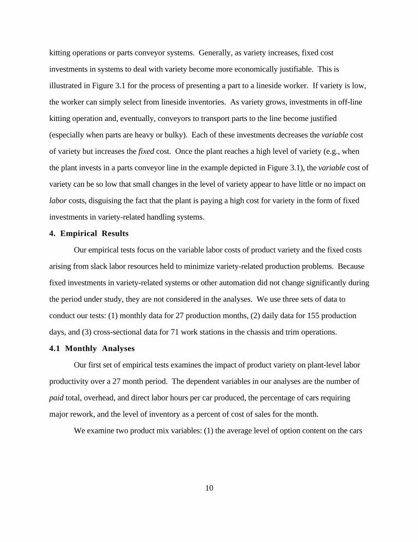
kitting operations or parts conveyor systems. Generally, as variety increases, fixed cost

investments in systems to deal with variety become more economically justifiable. This is

illustrated in Figure 3.1 for the process of presenting a part to a lineside worker. If variety is low,

the worker can simply select from lineside inventories. As variety grows, investments in off-line

kitting operation and, eventually, conveyors to transport parts to the line become justified

(especially when parts are heavy or bulky). Each of these investments decreases the variable cost

of variety but increases the fixed cost. Once the plant reaches a high level of variety (e.g., when

the plant invests in a parts conveyor line in the example depicted in Figure 3.1), the variable cost of

variety can be so low that small changes in the level of variety appear to have little or no impact on

labor costs, disguising the fact that the plant is paying a high cost for variety in the form of fixed

investments in variety-related handling systems.

4. Empirical Results

Our empirical tests focus on the variable labor costs of product variety and the fixed costs

arising from slack labor resources held to minimize variety-related production problems. Because

fixed investments in variety-related systems or other automation did not change significantly during

the period under study, they are not considered in the analyses. We use three sets of data to

conduct our tests: (1) monthly data for 27 production months, (2) daily data for 155 production

days, and (3) cross-sectional data for 71 work stations in the chassis and trim operations.

4.1 Monthly Analyses

Our first set of empirical tests examines the impact of product variety on plant-level labor

productivity over a 27 month period. The dependent variables in our analyses are the number of

paid total, overhead, and direct labor hours per car produced, the percentage of cars requiring

major rework, and the level of inventory as a percent of cost of sales for the month.

We examine two product mix variables: (1) the average level of option content on the cars

10

produced that month, and (2) the standard deviation in option content per car.1

Option Content. This variable equals the number of options on an average car from the

following list of 8 options: power door locks; power windows; cruise control; luggage

rack/spoiler; sun roof; two-tone paint; six cylinder engine; and five speed transmission. The

percentage of cars carrying these options is regularly reported to management due to their potential

disruptive impact on production. Let µi denote the fraction of cars that have option i, i = 1, ..., 8.

The mean option content then equals µi.

Option Variability. Our option variability measure equals the standard deviation in the number

of options per car. For i = 1, ..., 8 and a randomly selected car, the variable

1, if option i included xi =

0, otherwise

is a random variable with mean µi. However, because options are often bundled, the xi are not

independent which complicates computation of the standard deviation. Based on our discussions

with plant management about option bundling practices in the plant, we assume an inherent

hierarchy in the handling of options. If µi1 ≥ µ

i2, then any car with option i2 is assumed to have

option i1 as well. With this assumption, we can compute the fraction ρ

i of cars that have exactly i

options. Assume for notational simplicity that µ1 ≥ µ2 ... ≥ µ8. Then:

ρi = µi - µ1+i, i = 1, …, 7, ρ8 = µ8, and ρo - 1 - ρi - µ1

The standard deviation in the number of options per car equals

1We also examined the effect of model mix (four-door Corsica or two-door Beretta) on the dependentvariables. Greater production of the larger Corsica had a statistically significant negative impact on total andoverhead labor productivity but not on the other dependent variables. Moreover, the results for the other independentvariables changed little from those reported in the paper. Given the already small sample size, the ratio of Corsica toBerettas is not included in the reported results for the monthly tests.

11

The Option Content and Option Variability measures have a correlation of -0.31 (p < 0.01,

two-tailed), reflecting the reduction of option variability that occurs as more options are included as

standard equipment.

In addition to the product mix measures, three control variables are included in the

empirical tests:

Capacity Utilization. Since staffing for many overhead functions is relatively fixed in the

short-term, a capacity utilization variable is introduced to separate movements in labor hours per

car that are due to volume changes from those due to efficiency changes. The capacity utilization

measure is defined as the number of cars scheduled for production that month divided by the

plant's theoretical capacity in cars for the month.

Body Shop Uptime. Body shop uptime represents the percentage of available production time

that the body shop is operating. Body shop downtime is primarily due to mechanical problems that

are independent of the product mix produced by the plant. Because all downstream operations are

dependent on the body shop for the basic infrastructure of the car, these operations are idled if the

body shop is down for any length of time, lowering overall plant productivity. Consequently,

labor hours per car should be negatively related to body shop uptime.

Startup Month. The Wilmington plant was shut down for one month during the period under

study. In the following startup month, direct labor staffing was at normal capacity levels, but

actual production levels were intentionally held down to minimize startup problems. This variable

controls for the lower labor productivity during the startup month. The measure is coded one for

the startup month and zero otherwise.

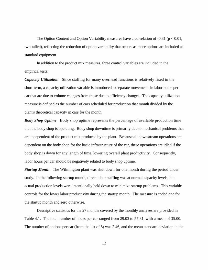
Descriptive statistics for the 27 months covered by the monthly analyses are provided in

Table 4.1. The total number of hours per car ranged from 29.03 to 57.81, with a mean of 35.00.

The number of options per car (from the list of 8) was 2.46, and the mean standard deviation in the

12

number of options per car was 2.15. Body shop uptime ranged from 77.69% to 97.88% (mean =

87.61%), with the major rework rate averaging 1.90% over the 27 months. The ratio of inventory

to cost of sales varied from 0.12 to 0.72 (mean = 0.26).

Table 4.2 provides the results from the monthly analyses. To control for autocorrelation,

the models are estimated in first differences. Durbin-Watson and Box-Pierce Q statistics indicate

that the remaining residuals approximate a stationary, white noise process. Moreover,

autocorrelation and partial autocorrelation correlograms reveal no spikes to suggest any remaining

systematic autoregressive or moving average component to the residuals.

Columns 1 through 3 examine the impact of product variety on labor hours per car. The

adjusted R2s range from 0.38 for overhead labor to 0.86 for direct labor. As predicted, direct

labor hours per car are negatively correlated with body shop downtime and positively correlated

with the startup month indicator. Total and overhead labor are lower when capacity utilization is

higher, supporting the notion of economies of scale in fixed overhead resources. More

importantly, the evidence indicates that greater option variety adversely impacts overhead

productivity but not direct labor. These results are consistent with Ittner and MacDuffie’s (1995)

cross-sectional study of auto assembly plants, which found that the number of options had a

significant negative impact on overhead hours per car, but was not significantly related to direct

labor requirements. While a car with more options clearly takes more time to assemble, our results

suggest that paid direct labor hours does not vary significantly with the number of options, an

issue we investigate further in later sections. Our findings do support claims in the management

accounting and operations management literatures that greater product variety increases overhead

requirements. The coefficients on option variability in the total and overhead labor models imply

that reducing option variability by 10% from its mean value reduces the number of hours required

to assemble a car by slightly more than one hour.

The evidence indicates that the negative consequences of option variety are related more to

13

the variability in option content rather than the mean number of options per car, a result consistent

with our field observations. If every car came loaded with all options, production planning,

material handling, and assembly procedures would be relatively straightforward. When variability

in option content is introduced into the plant, however, planning and scheduling becomes more

complex, sequencing and delivering the right parts to the line at the right time becomes more

difficult and the possibility of assembly errors increases, leading to higher overhead requirements.

Columns 4 through 6 of Table 4.2 examine the extent to which increases in major rework

account for the lower labor productivity in months with higher option variability. As shown in

Column 4, major rework as a percent of production is positively correlated with option variability

and negatively related to capacity utilization. The coefficient on option variability in the major

rework equation implies that reducing option variability by 10% from its mean value lowers major

rework by .158 or 8.3% from its average value over the 27 months. This evidence supports our

field research which indicated that greater option variability increases assembly defects.

Wilmington plant management indicated that the negative relation between capacity utilization and

variability reflects the fact that defects tend to decline with longer production runs. Since major

rework is performed by overhead personnel, it is not surprising that an increase in the rework rate

significantly increases overhead labor (Column 6) but has little impact on direct labor (Column 5).

The significant positive coefficient on option variability in equation (6) shows that option

variability’s impact on overhead functions extends beyond the additional overhead requirements

caused by increased major rework.

The relationship between product variety and inventory levels (as a percent of cost of sales)

is investigated in Column 7. Once again, the coefficient on option variability is positive and

statistically significant while mean option content continues to show no significant relationship

with the plant performance measures, supporting claims that higher product variety increases

inventory requirements. The coefficient on option variability indicates that reducing variability by

10% from its mean lowered inventory as a percent of cost of sales by 0.0215, or 8.27% from its

14

mean value. Additional analyses (not reported) indicate that the positive association between

inventory levels and option variability is due both to the increased number of cars in the major

rework area when variability is high, as well as to other variety-related factors such as increased

inventory requirements and contingencies.

4.2 Daily Analyses

The monthly analyses suggest that product variety impacts overhead labor per car, but is

not significantly associated with direct labor content. Our discussions with plant management

indicated that the insignificant associations between the product variety measures and direct labor in

the monthly tests is due in part to the availability of slack resources in direct labor operations. Our

direct labor measure represents the number of paid direct labor hours per car produced.

If the number of cars scheduled to be produced in a standard eight hour shift is less than the

plant's theoretical capacity, it may be possible to meet the shift's production schedule, for example,

in seven and a half hours, with assembly workers being paid for the entire eight hour shift. If

assembly problems are encountered, and the same production schedule takes anywhere between

seven and a half and eight hours to complete, no additional expense is incurred. Only when

production time is increased to more than eight hours is overtime required and direct labor workers

are paid for more than eight hours. Consequently, direct labor hours paid and hours worked may

not have a direct correspondence.

To examine this issue more closely, we gathered detailed production and direct labor data

for 151 production days. The plant provided us with the specific options included on every car

built during the period, paid direct labor hours in each assembly operation (body shop, paint,

chassis, trim, and final assembly), and total production line downtime. We calculated mean option

content and option variability based on 55 options (including two-door versus four-door) that the

plant uses in its assembly line sequencing algorithm. The variety measures reflect only those

options impacting the respective assembly operations (i.e., an option that affects work content in

chassis but not in trim is not included in the trim operation's variety measures). Two control

15

variables are included in the analyses: an indicator variable for the two production days following a

plant shutdown, and body shop downtime. The models are estimated in first differences to control

for autocorrelation.

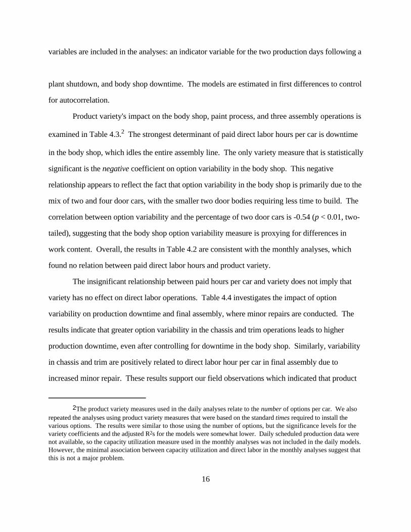
Product variety's impact on the body shop, paint process, and three assembly operations is

examined in Table 4.3.2 The strongest determinant of paid direct labor hours per car is downtime

in the body shop, which idles the entire assembly line. The only variety measure that is statistically

significant is the negative coefficient on option variability in the body shop. This negative

relationship appears to reflect the fact that option variability in the body shop is primarily due to the

mix of two and four door cars, with the smaller two door bodies requiring less time to build. The

correlation between option variability and the percentage of two door cars is -0.54 (p < 0.01, two-

tailed), suggesting that the body shop option variability measure is proxying for differences in

work content. Overall, the results in Table 4.2 are consistent with the monthly analyses, which

found no relation between paid direct labor hours and product variety.

The insignificant relationship between paid hours per car and variety does not imply that

variety has no effect on direct labor operations. Table 4.4 investigates the impact of option

variability on production downtime and final assembly, where minor repairs are conducted. The

results indicate that greater option variability in the chassis and trim operations leads to higher

production downtime, even after controlling for downtime in the body shop. Similarly, variability

in chassis and trim are positively related to direct labor hour per car in final assembly due to

increased minor repair. These results support our field observations which indicated that product

2The product variety measures used in the daily analyses relate to the number of options per car. We alsorepeated the analyses using product variety measures that were based on the standard times required to install thevarious options. The results were similar to those using the number of options, but the significance levels for thevariety coefficients and the adjusted R2s for the models were somewhat lower. Daily scheduled production data werenot available, so the capacity utilization measure used in the monthly analyses was not included in the daily models.However, the minimal association between capacity utilization and direct labor in the monthly analyses suggest thatthis is not a major problem.

16

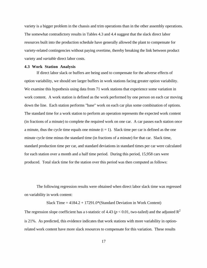
variety is a bigger problem in the chassis and trim operations than in the other assembly operations.

The somewhat contradictory results in Tables 4.3 and 4.4 suggest that the slack direct labor

resources built into the production schedule have generally allowed the plant to compensate for

variety-related contingencies without paying overtime, thereby breaking the link between product

variety and variable direct labor costs.

4.3 Work Station Analysis

If direct labor slack or buffers are being used to compensate for the adverse effects of

option variability, we should see larger buffers in work stations facing greater option variability.

We examine this hypothesis using data from 71 work stations that experience some variation in

work content. A work station is defined as the work performed by one person on each car moving

down the line. Each station performs "base" work on each car plus some combination of options.

The standard time for a work station to perform an operation represents the expected work content

(in fractions of a minute) to complete the required work on one car. A car passes each station once

a minute, thus the cycle time equals one minute (t = 1). Slack time per car is defined as the one

minute cycle time minus the standard time (in fractions of a minute) for that car. Slack time,

standard production time per car, and standard deviations in standard times per car were calculated

for each station over a month and a half time period. During this period, 15,958 cars were

produced. Total slack time for the station over this period was then computed as follows:

The following regression results were obtained when direct labor slack time was regressed

on variability in work content:

Slack Time = 4184.2 + 17291.0*(Standard Deviation in Work Content)

The regression slope coefficient has a t-statistic of 4.43 (p < 0.01, two-tailed) and the adjusted R2

is 21%. As predicted, this evidence indicates that work stations with more variability in option-

related work content have more slack resources to compensate for this variation. These results

17

support our field observations which indicated that assembly plants attempt to mitigate some of the

adverse effects of higher variety by building labor slack into the system, thereby introducing an

additional fixed cost of product variety.

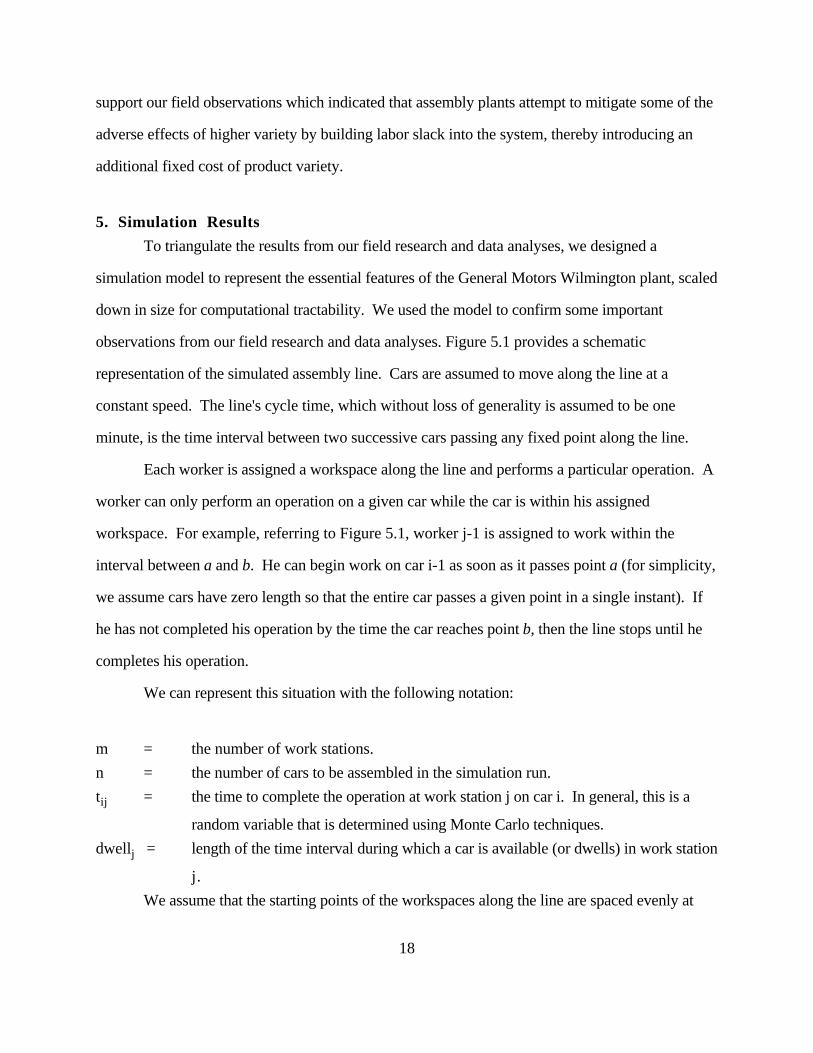
5. Simulation Results

To triangulate the results from our field research and data analyses, we designed a

simulation model to represent the essential features of the General Motors Wilmington plant, scaled

down in size for computational tractability. We used the model to confirm some important

observations from our field research and data analyses. Figure 5.1 provides a schematic

representation of the simulated assembly line. Cars are assumed to move along the line at a

constant speed. The line's cycle time, which without loss of generality is assumed to be one

minute, is the time interval between two successive cars passing any fixed point along the line.

Each worker is assigned a workspace along the line and performs a particular operation. A

worker can only perform an operation on a given car while the car is within his assigned

workspace. For example, referring to Figure 5.1, worker j-1 is assigned to work within the

interval between a and b. He can begin work on car i-1 as soon as it passes point a (for simplicity,

we assume cars have zero length so that the entire car passes a given point in a single instant). If

he has not completed his operation by the time the car reaches point b, then the line stops until he

completes his operation.

We can represent this situation with the following notation:

m = the number of work stations.

n = the number of cars to be assembled in the simulation run.

tij = the time to complete the operation at work station j on car i. In general, this is a

random variable that is determined using Monte Carlo techniques.

dwellj = length of the time interval during which a car is available (or dwells) in work station

j.

We assume that the starting points of the workspaces along the line are spaced evenly at

18

one minute intervals so that car i becomes available at work station j at time i + j - 2. Operation j

can begin on car i as soon after this time as the worker has completed operation j on car i-1. If the

operation is not completed by time i + j-2+dwellj, then the line stops until the operation is

completed.

In our primary method for generating tij, the work stations were segmented into two

categories depending on whether the workstation installed an option or not. We assume there are k

possible options. Option j is installed at a single workstation ij, requires OTj minutes and occurs

on a given car with probability pj. We set OTj = 1/pj and dwellj = OTj, so that the average

operation time is 1 and dwellj is long enough for the operation on a car with an option to be

completed without stopping the line. Note, however, that if two or more options occur in

succession, the worker would get behind and the line would stop.

In a particular simulation, tij for option-related work stations are set by Monte Carlo

generation of the option configuration of each car. For all of the remaining work stations and cars,

we set dwellj = tij = 1 for all i. These work stations would not cause line stoppage.

After tij were generated for a sample of n cars, we determined an assembly sequence for

the n cars that was intended to evenly space the occurrence of options at work stations. To be

more precise, let nj denote the number of times an option occurs at work station j in a sample of n

cars (in expectation nj = n pj, but in a particular sample of cars nj could differ from this value due

to randomness). In an ideal sequence, a car requiring an option should arrive at work station j

every n/nj cycles. For example, if n = 15 and five cars require an option at work station 1, then the

start times for these cars should be 0, 3, 6, 9 and 12. If this sequencing can be achieved for all

option-related work stations and the number of cars with options does not exceed pj n, then all

operations can be performed without line stoppage.

19

Our sequencing rule attempts to create a sequence that comes as close as possible to this

ideal case by choosing a next car in the sequence from the unsequenced cars that maximizes a

sequence score that equals the sum of the times by which the start time of each option on that car

would exceed the start time of an ideal sequence. Note that the score for a car can be negative if

choosing the car would result in options re-occurring in too short an interval. Most auto plants use

sequencing algorithms similar to this, with the algorithms applied each day to the set of cars

scheduled for assembly that day. To simulate the daily sequencing that occurs in the real world,

we assumed that the n cars in a simulation correspond to a fixed number of daily batches and

applied the sequencing algorithm to each daily batch of cars. In all of our runs, m = 50, n = 2000

and the number of days equaled 10. Hence, the sequencing algorithm was applied to successive

daily batches of 200 cars in the 2000 car simulated sample. These cars can be processed in 2050

cycles. We ignored the first 50 and last 50 cycles since they correspond to situations in which the

line is not completely loaded.

In all of our simulations, all pj were set to a common value p and the work stations affected

by options were [mj/k], j = 1, ..., k. Forty different values for k and p were simulated using the

following values: (1) p = .5 and k = 1, ..., 10; (2) k = 5 and p = .25, .3, .35, ..., .7; (3) k = 1...,

10 and p chosen so that the standard deviation in total labor content (σtime

) was equal to 3; and (4)

k = 1, ..., 10 and p chosen so that the standard deviation of the number of options (σcount

) was

equal to .5. It is easy to show that σtime

= √k(1-p)/p and σcount

= √k p (1-p). For each of these

cases we tabulated the total time that the line was stopped and used this to compute the percentage

increase in labor content due to line stoppage. To compute the percentage increase in direct labor,

we note that total labor with no stoppage over the simulated time is 50 x 1950 and the time lost due

to stoppage is 50 times the total time that the line is stopped.

20

For each of these cases, we also experimented with buffering those operations affected by

options with additional capacity. We ignored the integrality constraint on capacity imposed by

workers and assumed that capacity could be expanded continuously with a proportionate reduction

in operation times. Note that increasing capacity at all option-related work stations by a certain

percentage increases the amount of labor assigned to the work station by the same percentage, but

red uces the additional labor required due to line stoppage. We used Fibinacci search to find

the optimal buffering level in each case simulated and computed the resulting percentage increase in

total labor content due both to buffering and line stoppage.

Our field observations indicated that random contingencies are another source of variability

in plants due to factors such as defective parts or work on preceding operations that is performed

incorrectly. Because these random contingencies can also cause line stoppage, we sought to

compare the amount of line stoppage caused by option variability to an equivalent amount of

purely random variability. To do this, we made a run for each simulated case in which all tij were

chosen uniformly from the interval [1 - ∆,1 + ∆]. Note that the standard deviation in labor content

is given by σtime

= √m ∆3 /3. We used this result to choose a ∆ that would equalize σtime

in

the random case with σtime

in the corresponding option case.

The results from the 40 simulation runs are provided in Table 5.1. The first set of runs

held the probability of an option constant at 0.50, but varied the number of options from 1 to 10.

Standard deviations in both work content time and the number of options increase as the number of

available options goes up. Consistent with the empirical tests, this increased variability is

accompanied by greater direct labor content due to increased line stoppage. However, buffering

the line with additional labor capacity reduced the productivity losses due to line stoppage,

providing theoretical support for the buffering observed in the Wilmington plant.

The second set of runs held the number of options constant at 5 but varied the probability

21

that an option would be included on a car from 0.25 to 0.70. As the probability of an option being

included increased, the standard deviation in work time decreased. The standard deviation in

option counts, however, first increased and then fell as option penetration reached 0.60 or greater.

Line stoppages in both the buffered and unbuffered simulations followed a pattern similar to the

pattern in option counts, first increasing and then decreasing, with the peak line stoppage

percentages occurring when option penetration ranged from approximately 0.45 to 0.60. These

results suggest that assembly plants are better off when options are installed on only a small

fraction of cars or on a large percentage of car, supporting the industry practice of installing many

"options" as standard equipment on most cars. Once again, the buffered line experienced

significantly fewer line stoppages than the unbuffered line, a result consistent with the empirical

evidence.

In the third set of tests, both the number of options and the probability that an option is

installed are varied so that the standard deviation in work content remains equal to 3.00. Although

the variability in work content remains the same, the standard deviation in option counts increases

with the number of options, as does the amount of line stoppage in both the buffered and

unbuffered simulations. Our field research made it clear why this happens. If only one option is

offered, it would be easy to achieve a sequence of perfectly spaced options. As the number of

options grow, however, a plant is prevented from doing this because the ideal sequence for one

work station may not be the ideal sequence for another. Consequently, the probability that a

worker will encounter a sequence of cars that cannot be completed in the allowable cycle time

increases, causing line stoppages or rework to increase.

In the fourth set of tests, the number of options and the probability that an option is

installed are varied so that the standard deviation of option count remains constant at 1. The fact

that the percent increase in labor content with buffering is essentially constant at 2-3% for these

runs further establishes that the standard deviation of option counts is the principal driver of lost

direct labor productivity due to options.

22

In all of the simulations, random variability caused a significantly greater percentage

increase in labor content than option variability. These results suggest that the impact of option

variability can be partially mitigated by sequencing cars to space options. In contrast, random

variability cannot be anticipated, indicating that auto manufacturers should be even more zealous in

their attack on random variability than they are in trying to reduce option variability. It is not clear

that all auto manufacturers are following this logic.

To better understand the role of option "bundling" on direct labor productivity, we repeated

all the experiments assuming that options were bundled. That is, a given car either had all options

or no options. With bundling, it is easier to obtain a sequence that perfectly spaces options since

there are only two categories of cars, those with no options or those with all options. As a result,

we would expect the percentage increase in labor content to be reduced by bundling. This is

confirmed in Table 5.2, especially in the buffered case.

6. Conclusion

Prior research on the relationship between product variety and manufacturing performance

has provided conflicting results. In contrast to previous studies, we employ three sources of data

to develop and test hypotheses regarding the impact of variety on automobile assembly. The field

evidence, data analyses, and simulation models allow us to triangulate the findings and provide

deeper insight into the various means through which variety affects productivity.

Our results provide a number of implications for future research. First, the distinction

between fixed and variable costs of variety is an important one that has received relatively little

attention in the academic literature. If plants have invested in fixed resources that minimize the

adverse effects of product variety, studies examining the statistical association between variety and

productivity can find little impact from high variety, even though significant fixed costs have been

incurred due to higher product variety.

The evidence also indicates that the manufacturing variability introduced by higher product

variety has a greater impact on productivity than the number of product variations. If a large

23

number of options are installed on all cars, production planning and material handling are

straightforward, and the production task facing the line worker does not vary by vehicle. In

contrast, greater variability increases the complexity of production planning and material handling

activities and raises the probability of defects and downtime. Consequently, simple proxy

variables for variety such as the number of parts or number of products may not allow researchers

to capture the impact of variety on manufacturing performance.

Although research on assembly line balancing has a long history in the management science

literature, little research has examined line balancing issues in mixed-model assembly operations

such as an automobile assembly line. Our evidence suggests that line balancing provides only a

partial solution to the product variety problem in these settings. Although labor buffers and kitting

operations (which make product variety transparent to the assembly worker by sequencing parts

off line) can help to alleviate variety-related contingencies, they introduce additional fixed costs into

the system. Additional research on line balancing in mixed-model assembly operations can help to

minimize the variety-related losses that currently plague automobile manufacturers.

Finally, although variety-related variability is found to reduce productivity, our field

observations and simulation results suggest that random variability is even more disruptive to

factory operations. Although the impact of option variability can be mitigated to a certain extent by

line sequencing and option bundling, reducing random variability requires organizational changes

that extend beyond the technical solutions used to minimize the effects of option variability.

ACKNOWLEDGEMENT

We’re grateful to the many people at the General Motors Wilmington Auto Assembly Plantwho provided access to plant and to the data required for this study, and who helped us tounderstand the plant operations. We are particularly grateful to Tom Brennan, Material Manager,who was our primary contact at the plant and to Ralph Harding who was Plant Manager at the timeof the study. We appreciate the research assistance provided by Taylor Randall, Bill Webb andKannan Sethuraman. The comments of Robert Kaplan and seminar participants at HarvardUniversity are also appreciated. The work of the first author was supported in part by the NationalScience Foundation and General Motors under industry/academia collaborative grant NSF SES91-09798. The work of the second author was supported by KPMG Peat Marwick.

24

25

REFERENCES

ANDERSON, S.W., “Measuring the Impact of Product Mix Heterogeneity on ManufacturingOverhead Cost,” Accounting Review, Vol. 70, No. 3, July 1995, pp. 363-387.

BANKER, R., POTTER, G., and SCHROEDER, R.G., “An Empirical Analysis ofManufacturing Overhead Cost Drivers,” working paper, University of Minnesota, 1993.

COOPER, R. and KAPLAN, R.S., “The Design of Cost Management Systems, EnglewoodCliffs, NJ, Prentice Hall, 1991.

FISHER, M., JAIN, A., and MAC DUFFIE, J.P., “Strategies for Product Variety: Lessons fromthe Auto Industry,” in Redesigning the Firm, edited by B. Kogut and E. Bowman, New York:Oxford University Press, pp. 116-154.

FOSTER, G. and GUPTA, M., “Manufacturing Overhead Cost Driver Analysis,” Journal ofAccounting and Economics, March 1989, pp. 310-337.

HAYES, R. and WHEELWRIGHT, S., “Restoring Our Competitive Edge, New York, NY, JohnWiley & Sons, 1984.

ITTNER. C. and KOGUT, B., “How Control Systems Can Support Organization Flexibility,” inRedesigning the Firm, edited by B. Kogut and E. Bowman, New York: Oxford University Press,1995, pp. 155-180.

ITTNER, C. And MAC DUFFIE, J.P., “Explaining Plant-Level Differences in ManufacturingOverhead: Structural and Executional Cost Drivers in the World Auto Industry,” Production andOperations Management, Vol. 4, No. 4, Fall 1995, pp. 312-334.

KEKRE, S. And SRINIVASAN, K., “Broader Product Line: A Necessity to Achieve Success?,”Management Science, Vol. 36, No. 10, October 1990, pp. 1216-1231.

MAC DUFFIE, J.P., SETHURAMAN, K. and FISHER, M., “Product Variety andManufacturing Performance: Evidence from the International Automotive Assembly Plant Study,”forthcoming in Management Science, 1996.

MILLER, J.G. and VOLLMAN, T.E., “The Hidden Factory,” Harvard Business Review, Sept-Oct 1963, pp. 142-150.

SKINNER, W., “The Focused Factory,” Harvard Business Review, Vol. 52, No. 3, 1974, pp.113-121.

26

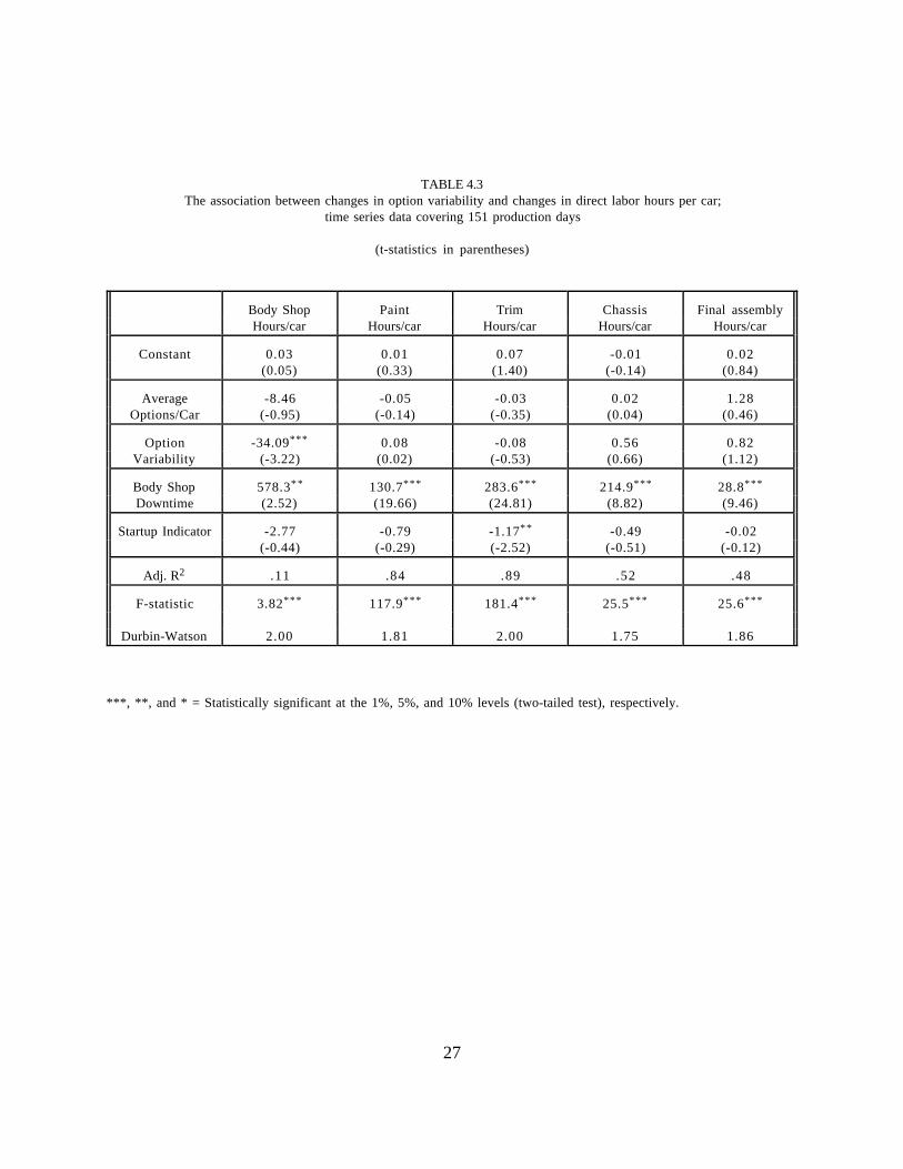
TABLE 4.3The association between changes in option variability and changes in direct labor hours per car;

time series data covering 151 production days

(t-statistics in parentheses)

Body ShopHours/car

PaintHours/car

TrimHours/car

ChassisHours/car

Final assemblyHours/car

Constant 0.03(0.05)

0.01(0.33)

0.07(1.40)

-0.01(-0.14)

0.02(0.84)

AverageOptions/Car

-8.46(-0.95)

-0.05(-0.14)

-0.03(-0.35)

0.02(0.04)

1.28(0.46)

OptionVariability

-34.09***

(-3.22)0.08

(0.02)-0.08

(-0.53)0.56

(0.66)0.82

(1.12)

Body ShopDowntime

578.3* *

(2.52)130.7***

(19.66)283.6***

(24.81)214.9***

(8.82)28.8***

(9.46)

Startup Indicator -2.77(-0.44)

-0.79(-0.29)

-1.17* *

(-2.52)-0.49

(-0.51)-0.02

(-0.12)

Adj. R2 .11 .84 .89 .52 .48

F-statistic

Durbin-Watson

3.82***

2.00

117.9***

1.81

181.4***

2.00

25.5***

1.75

25.6***

1.86

***, **, and * = Statistically significant at the 1%, 5%, and 10% levels (two-tailed test), respectively.

27

TABLE 4.4

The association between changes in option variability and changes in production downtime and final assembly hours percar;

time series data covering 151 production days

(t-statistics in parentheses)

Total Downtime(% of Production Time)

Final AssemblyHours/Car

Constant 0.003*

(1.97)-0.006(-0.04)

Body Shop Downtime 0.642***

(18.95)29.12***

(17.21)

Startup Indicator 0.0001(0.11)

0.043(0.58)

Option Variability--Body Shopa -0.003(-1.36)

-0.180(-0.91)

Option Variability--Paint -0.001(-0.71)

-0.027(-0.13)

Option Variability--Trim 0.004***

(2.93)0.031*

(1.80)

Option Variability--Chassis 0.022* *

(2.33)0.19***

(2.61)

Option Variability--Final Assembly 0.006(1.57)

0.437(1.57)

Adj. R2 .93 .87

F-statistic

Durbin-Watson

170.0***

1.97

88.01***

1.76

***, **, and * = Statistically significant at the 1%, 5%, and 10% levels (two-tailed test), respectively.

a. Variability measures pertain to options impacting that particular process step.

28

Table 5.1 Simulation Results

2000 cars, 50 work stations, 10 days Mean time = 50 minutes.Standard Deviation - Time is in minutes

Percent Increase in Labor Content

Number of Prob of an Standard Deviations Options option Time Count Unbuffered Buffered Random*

1 0.50 1.00 0.50 2 2 25 2 0.50 1.41 0.71 3 3 35 3 0.50 1.73 0.87 7 5 43 4 0.50 2.00 1.00 13 8 49 5 0.50 2.24 1.12 18 10 55 6 0.50 2.45 1.22 23 12 60 7 0.50 2.65 1.32 27 14 65 8 0.50 2.83 1.41 29 16 69 9 0.50 3.00 1.50 31 18 74 10 0.50 3.16 1.58 34 20 77

5 0.25 3.87 0.97 14 7 95 5 0.30 3.42 1.02 15 8 84 5 0.35 3.05 1.07 17 7 75 5 0.40 2.74 1.10 19 9 67 5 0.45 2.47 1.11 17 10 61 5 0.50 2.24 1.12 18 10 55 5 0.55 2.02 1.11 23 8 50 5 0.60 1.83 1.10 23 7 45 5 0.65 1.64 1.07 22 5 40 5 0.70 1.46 1.02 20 4 36

1 0.10 3.00 0.30 6 1 74 2 0.18 3.00 0.55 8 2 74 3 0.25 3.00 0.75 8 3 74 4 0.31 3.00 0.92 12 6 74 5 0.36 3.00 1.07 19 8 74 6 0.40 3.00 1.20 21 13 74 7 0.44 3.00 1.31 23 16 74 8 0.47 3.00 1.41 25 17 74 9 0.50 3.00 1.50 31 18 74 10 0.53 3.00 1.58 33 18 73

* Random chooses all process times uniformly in the interval 1-delta, 1+delta, where delta chosen to givesame standard deviation as the unbuffered and buffered cases.

29

Table 5.2 Simulation Results with Bundled Options

2000 cars, 50 work stations, 10 days Mean time = 50 minutes.Standard Deviation - Time is in minutes

Percent Increase in Labor Content

Number of Prob of an Standard Deviation Options option Time Count Unbuffered Buffered

1 0.50 1.00 0.50 1 1 2 0.50 2.00 1.00 2 2 3 0.50 3.00 1.50 1 1 4 0.50 4.00 2.00 2 2 5 0.50 5.00 2.50 2 2 6 0.50 6.00 3.00 3 3 7 0.50 7.00 3.50 7 7 8 0.50 8.00 4.00 7 7 9 0.50 9.00 4.50 8 8 10 0.50 10.00 5.00 2 2

5 0.25 8.66 0.30 4 3 5 0.30 7.64 0.77 7 1 5 0.35 6.81 1.30 11 4 5 0.40 6.12 1.85 11 3 5 0.45 5.53 2.40 8 1 5 0.50 5.00 2.94 2 2 5 0.55 4.52 3.47 18 8 5 0.60 4.08 3.99 15 7 5 0.65 3.67 4.50 18 5 5 0.70 3.27 4.99 18 4

1 0.10 3.00 2.17 9 1 2 0.18 4.24 2.29 5 0 3 0.25 5.20 2.38 4 2 4 0.31 6.00 2.45 6 1 5 0.36 6.71 2.49 11 4 6 0.40 7.35 2.50 12 3 7 0.44 7.94 2.49 10 2 8 0.47 8.49 2.45 6 1 9 0.50 9.00 2.38 8 8 10 0.53 9.49 2.29 20 6

30

31