Opportunistic Sharing Single Radar and Cellularpeha/Opportunistic_Sharing__Single... · ATC radar (rotating horizontally with a constant speed), in a sharing scheme based only on

IEEE Journal on Selected Areas in Communications, Nov. 2012

1

Abstract—This paper considers opportunistic primary-

secondary spectrum sharing when the primary is a rotating

radar. A secondary device is allowed to transmit when its

resulting interference will not exceed the radar’s tolerable level,

in contrast to current approaches that prohibit secondary

transmissions if radar signals are detected at any time. We

consider the case where an OFDMA based secondary system

operates in non-contiguous cells, as might occur with a

broadband hotspot service, or a cellular system that uses

spectrum shared with radar to supplement its dedicated

spectrum. It is shown that even fairly close to a radar, extensive

secondary transmissions are possible, although with some

interruptions and fluctuations as the radar rotates. For example,

at 27% of the distance at which secondary transmissions will not

affect the radar, on average, the achievable secondary data rates

in down- and upstream are around 100% and 63% of the one

that will be achieved in dedicated spectrum, respectively.

Moreover, extensive secondary transmissions are still possible

even at different values of key system parameters, including cell

radius, transmit power, tolerable interference level, and radar

rotating period. By evaluating quality of service, it is found that

spectrum shared with radar could be used efficiently for

applications such as non-interactive video on demand, peer-to-

peer file sharing, file transfers, and web browsing, but not for

applications such as real-time transfers of small files and VoIP.

Index Terms — Coexistent, Cooperative, Opportunistic,

OFDMA, Primary-secondary spectrum sharing, Radar

I. INTRODUCTION

RIMARY-SECONDARY spectrum sharing can substantially

alleviate spectrum scarcity [1]. Radars could be a good

candidate for the primary systems in spectrum sharing because

they operate in a large amount of spectrum. For example, in

the US over 1.7 GHz of spectrum from 225 MHz to 3.7 GHz

“involves radar and/or radionavigation infrastructure," [2] and

Manuscript received January 5, 2012; revised June 3, 2012. This work was

supported by the Fundação para a Ciência e a Tecnologia (Portuguese Foundation for Science and Technology) through the Carnegie Mellon -

Portugal Program under Grant SFRH/ BD/33594/2008.

R. Saruthirathanaworakun is a Ph.D. student in the Carnegie Mellon – Portugal program, with Department of Engineering and Public Policy,

Carnegie Mellon University, Pittsburgh, PA 15213 USA, and with Instituto

Superior Técnico – Technical University of Lisbon, Portugal (phone: (+351) 218-418-199; fax: (+351) 218-418-291; e-mail: [email protected]).

J.M. Peha is with the Dept. of Engineering and Public Policy and the Dept.

of Electrical and Computer Engineering, Carnegie Mellon University (e-mail: [email protected]).

L.M. Correia is with Instituto Superior Técnico/Instituto de

Telecomunicações – Technical University of Lisbon (e-mail: [email protected]).

around 1.1 GHz of this 1.7 GHz is used by fixed land-based

radars in non-military applications [3].

This paper considers opportunistic sharing where a

secondary device can transmit only when its transmissions

will not cause harmful interference, i.e., interference that

causes noticeable service disruption to the primary [4].

Currently, there are some bands in which radars are

protected from harmful interference by granting them

exclusive rights to operate in a given area and frequency band,

and other bands (e.g., at 5 GHz) in which radars share

spectrum with unlicensed devices that can transmit only if

they are so far from any radar that the radar is undetectable

[5]. Both of these are white space approaches to primary-

secondary sharing, where secondary wireless systems are

allowed to operate in frequency bands and geographic regions

that are found to be entirely “unused” by any primary system.

In contrast, with the gray space sharing [6] considered in this

paper, a secondary device is allowed to transmit near a radar,

but only when and with a transmit power that will not cause

harmful interference. The maximum transmit power of

secondary devices changes over time, based on the behavior of

the primary system. We have previously used this approach to

prevent a secondary spectrum user from causing harmful

interference to a primary user, when the primary was a cellular

system [7]. Dynamic power control has long been used to

control devices within a single communication system, e.g., a

cellular network, but here it is used to allow systems under

different administrative control to share spectrum in a

primary-secondary arrangement.

We investigate how much the secondary system can

transmit with this different sharing concept, by considering

sharing with a rotating radar. Examples of these radars

include applications in weather operating in [2.7, 3.0] GHz,

Air Traffic Control (ATC) in [2.7, 2.9] GHz, and other

surveillance in [0.42, 0.45] GHz and [2.7, 3.5] GHz [3]. With

a rotating main beam, the radar antenna gain seen by the fixed

secondary device varies, hence, there will be periods of time

when the link loss (including antenna gains and path loss)

between the device and the radar is high enough so that the

device can transmit successfully, without causing harmful

interference to the radar. This sharing can be either

cooperative (through explicit coordination between the

secondary device and the primary system) or coexistent

(without coordination) [1].

The case where a secondary system operates in non-

Opportunistic Sharing between Rotating Radar

and Cellular

Rathapon Saruthirathanaworakun, Student Member, IEEE, Jon M. Peha, Fellow, IEEE, and

Luis M. Correia, Senior Member, IEEE

P


2

adjacent cells is considered; two examples are a secondary

system providing broadband hotspots, and a cellular system

using shared spectrum when a traffic surge temporarily

exceeds what can be supported in dedicated spectrum..

Only a few previous studies have addressed spectrum

sharing with a rotating radar. Marcus qualitatively discussed

the possibility in [8]; Wang et al. [9], and later Rahman and

Karlsson [10], analyzed coexistent sharing quantitatively, but

only when a device is far enough that its transmissions will not

cause harmful interference even in the radar’s main beam, as

occurs in 5 GHz band. Instead, the proposed sharing makes

use of the varying link loss between the radar and a secondary

device, hence, a device may transmit at a closer distance to the

radar, but with some interruptions and fluctuations in

transmissions as the radar rotates.

We quantify the extent of secondary transmissions, and

characterize the effect of interruptions and fluctuations on

secondary transmissions. Performance is analyzed for six

applications from the four classes of services [11]: 1) Voice-

over-IP (VoIP, conversational), 2) non-interactive video on

demand (streaming), 3) Peer-to-Peer file sharing (P2P,

background), 4) automatic meter reading (e.g., electricity

meter reading, background), 5) file transfer (interactive, with

traffic in both up- and downstreams), and 6) web browsing

(interactive, with traffic mostly in downstream).

The sharing scenario is described in Section II. The power

level that a secondary device will be allowed to transmit and

the resulting SINR (Signal to Interference plus Noise Ratio)

are derived in Section III. Parameters used to evaluate

performance of the sharing, numerical results, and conclusions

are discussed in Sections IV, V, and VI, respectively.

II. SPECTRUM SHARING SCENARIO

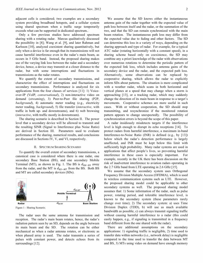
To quantify the overall extent of secondary transmissions, a

canonical case is considered where there is one radar, one

secondary Base Station (BS), and one secondary Mobile

Terminal (MT), as shown in Fig. 1. The BS is �� away

from the radar, and the MT is �� from the BS. Both BS

and MT are called secondary devices (SDs).

Figure 1 - Sharing Scenario.

The radar uses the same antenna for transmission and

reception. The radar’s main beam rotates, hence, the radar’s

radiation pattern seen by an SD, depends on the angle between

its main beam and the SD. The rotation can be either

mechanical as when a radar antenna rotates, or electronic as

when phased array is used. The radar transmits a series of

pulses with constant power, and detects echoes from its

surroundings [12].

We assume that the SD knows either the instantaneous

antenna gain of the radar together with the expected value of

path loss between itself and the radar, or the summation of the

two, and that the SD can remain synchronized with the main

beam rotation. The instantaneous path loss may differ from

the expected value due to fading and other factors. The SD

can determine this loss in a variety of ways, depending on the

sharing approach and type of radar. For example, for a typical

ATC radar (rotating horizontally with a constant speed), in a

sharing scheme based only on coexistence, the SD may

combine any a priori knowledge of the radar with observations

over numerous rotations to determine the periodic pattern of

the expected link loss, which includes antenna gains of the

secondary device and the radar, and the expected path loss.

Alternatively, some observations can be replaced by

cooperative sharing, which allows the radar to explicitly

inform SDs about patterns. The situation is more complicated

with a weather radar, which scans in both horizontal and

vertical planes at a speed that may change when a storm is

approaching [13], or a tracking radar, which may suddenly

change the direction of its main beam in response to a target’s

movements. Cooperative schemes are more useful in such

cases. With or without cooperation, the SD should stop

transmitting, and resynchronize if the monitored rotation

pattern appears to change unexpectedly. The possibility of

synchronization errors is beyond the scope of this paper.

A radar insidiously misdetects targets if the interference

level is high enough to disrupt its echo receptions [14]. To

protect radars from harmful interference, a maximum in-band

Interference-to-Noise Ratio (INR) is defined (e.g., by [13])

below which the radar’s detection performance is largely

unaffected, and INR must be kept below this limit with

sufficiently high probability. Many radar systems are used in

applications that affect people’s lives, so preventing harmful

interference in these cases is especially important. For

example, recently in the UK there has been discussion on the

risk of inadvertent interference to aviation radars operating in

the 2.7 GHz band from LTE operating in 2.6 GHz [15].

We assume that the secondary system uses Orthogonal

Frequency Division Multiple Access (OFDMA), which is used

in wireless communication systems such as LTE. However,

the proposed sharing model could be applicable to other

secondary systems as well. The proposed sharing model

assumes that: 1) Some information of the radar, such as pulse

power, rotating period, and tolerable interference level, is

known to the secondary system (these parameters rarely

change over time); 2) The secondary system: a) uses Time

Division Duplex (TDD), b) will use as much available

bandwidth as possible, c) can always transmit signaling traffic

without causing harmful interference to a radar (this could

easily happen, e.g., if signaling is transmitted in a frequency

band different from the one shared with the radar).

There are additional assumptions on the secondary

applications: 1) signaling traffic is negligible, 2) time used to

transfer data within networks (i.e., network delay) is negligible

compared to the time used to transfer the data between MT

and BS, 3) MTs using video on demand have enough memory


3

for buffering, and a constant streaming rate is used.

III. SECONDARY MAXIMUM ALLOWABLE TRANSMIT POWER

AND ACHIEVABLE SINR

An SD determines its maximum allowable transmit power,

�,�� , from the radar’s tolerable level �� (which is known to

the SD, assumption 1 in Section II), and the expected link loss

between itself and the radar, which varies depending on

azimuthal angle between the radar’s main beam and the

device, �. When one secondary transmitter is using as much

bandwidth as possible (assumption 2), from �� , the SD at

distance �� from a radar can determine �,�� as

�,�� , �� = ��

�� !�,"#$%�&,�"#$%� , �,'(��_�� *, (1)

where �,'(��_�� is the SD’s transmit power limit, and

+!�,��, �� is the link loss, between the radar and the

transmitter, that the transmitter expects. As discussed in

Section II, there are various ways that an SD can determine

+!�,��, e.g., when coexistent sharing is employed, +!�,��

could be estimated during a start-up phase by averaging over

repeated samples of instantaneous link loss between the radar

and the SD. Margin ,- provides interference protection for

any difference between the instantaneous path loss and the one

expected by the SD, including differences from signal fading

and from any measurement error during the start-up phase.

When the difference from the expected path loss is high, to

keep the probability of harmful interference at a particular

small level, a higher margin will be needed; this higher margin

will result in more conservative extent of secondary

transmissions. Even with an adequate margin, gray space

sharing inherently introduces some risks that are not presented

with white-space sharing, e.g., the power control mechanisms

in a secondary system might be hacked and made to interfere

with the primary system, or some system bug might cause a

secondary transmitter to inaccurately calculate �,�� . To

mitigate the effects of interference in such cases, a new

approach to regulation and governance is required, which is

beyond the scope of this paper, but discussed in [6], [16].

From (1), it is possible to calculate SDs’ SINR, .�, which

will in turn determine achievable data rates. This calculation

is based on the conservative assumption that the time between

radar pulses during which the secondary will not experience

interference from the radar (which is typically less than 1 ms

[13]) can be neglected. When a secondary transmitter and

receiver are ��/ and ��/ away from the radar, and the

secondary transmitter and receiver are ��/��/ apart, .� is

.��, ��/, ��/ , ��/��/� = �,%��01$"1�×3%,456�&,�"#$01�7%8%9 �,"#$%�&,�"#$"1�×3"#

(2)

where +�,��/��/� is link loss between the secondary

transmitter-receiver pair, �� is background noise power

spectral density at the secondary receiver, and :� is a

secondary bandwidth per user.

IV. PARAMETERS FOR EVALUATING THE EXTENT OF

SECONDARY TRANSMISSIONS

The parameters used to evaluate the performance of

spectrum sharing with radar are: 1) secondary data rate, ;<,�,

calculated from .�; 2) fraction of time that the SD can achieve

a required data rate ;<,='(; and 3) statistics and distribution of

time that ;<,� < ;<,='(, i.e., interrupted time.

From the SINR in (2), the resulting ;<,��.�� is calculated

using a set of equations, obtained from regression analyses on

3GPP data [17]. The data are obtained assuming 1) an urban

or suburban environments with fairly small cell and low delay

spread (i.e., Extended Pedestrian A channel model); 2) a very

low speed user (i.e., 5-Hz Doppler frequency); and 3) Multiple

Input Multiple Output 2 × 2 in both up- and down-streams.

The resulting ;<,��.�� will be the maximum rate obtained

among QPSK, 16QAM, and 64QAM modulation schemes.

From (2), ;<,� varies periodically, and is a function of

�, ��/ , ��/ , and ��/��/. For a given ;<,='( , the

interrupted time together with its statistics, and the fraction of

time that ;<,� ≥ ;<,='(, A�B,%C�B,DEF, in a rotating cycle is:

A�B,%C�B,DEF =G HI"B,%J"B,DEF,KL∀K

�"# , (3)

where N�B,%C�B,DEF,K is the �-th period (in a rotating cycle) that

;<,� ≥ ;<,='(, and O�� is the rotating period.

Different service classes require different quality

measurements [11]. For the considered applications, different

parameters are used to evaluate performance: 1) VoIP requires

a symmetric constant data rate ;<,P��3 in both up- and

downstreams, and an interrupted time NP��3 lower than an

acceptable level; 2) Video on demand initially requires an

average downstream rate over a rotating cycle ;<,�!!!!! larger than

the constant streaming rate ;<,PQ�'�; as a buffer is used to

maintain streaming continuity, the probability that the buffer

will be empty is also evaluated; 3) P2P, file transfer, web

browsing, and meter reading, require no minimum data rate. ,

For P2P and file transfers, achievable data rate is an

appropriate measure. For an interactive application like web

browsing, webpage download time is our measure.

For VoIP, samples of NP��3 across a rotating cycle, and its

distribution, were obtained from instantaneous secondary data

rate and ;<,P��3. As VoIP is bi-directional, instantaneous

secondary data rate for VoIP is the minimum of the up- and

downstream values.

For video on demand, given the amount of data needed for

initial buffering, R<S_Q7Q�, the amount of data buffered at time T after streaming starts (or resumes) R<S�T, T-�� is

R<S�T, T-�� = R<S_Q7Q� + V ;<,�,W�TX��YZ�� TX − ;<,PQ�'�, (4)

where ;<,�,W�TX� is the instantaneous downstream secondary


4

data rate, and T-� is the streaming starting time.

From (4), for a given start time T-�,Q, one can determine if

and when the buffer would be empty. Based on multiple

values of T-�,Q across a rotating cycle, the probability that the

buffer will be empty, i.e., probability of interruptions, AQ7�=\,

during streaming can be obtained from:

AQ7�=\ = G ]^K_`��Kabc��

, (5)

where dQ is a binary variable that equals 1 if R<S = 0, and 0

otherwise. e�� is the total number of T-�,Q considered. Note

that video on demand operates when ;<,�!!!!! > ;<,PQ�'�, hence, if

R<SgT, T-=�,Qh ≠ 0 in a rotating cycle, it will never go to zero

during streaming.

For P2P, file transfer, web browsing, and meter reading, a

wide range of file sizes is transferred. Because secondary

transmissions can be interrupted, files of different sizes

experience different perceived data rates ;<,�,\�T-��, which

depend on when a file is transferred T-�.

;<,�,\�T-�� = Pk�k�� , (6)

where RS is size of a file, and OS�T-�� is the time that an SD

uses to transfer the file, i.e. file transfer time. Distribution of

;<,�,\ can be obtained by choosing different T-�’s.

V. NUMERICAL RESULTS

Parameters used to obtain numerical results are summarized

in Section A. The performance of secondary transmissions

averaged across a cell is evaluated in Section B; this average

performance is measured in terms of both mean data rate and

percentage of time that a secondary device can transmit.

Performance for video on demand and VoIP are evaluated in

Sections C and D, respectively. The characteristics and

performance of secondary transmissions for file upload- and

downloading services are shown in Section E. We investigate

sensitivity of these results on important system parameters

including (secondary) cell radius, radar transmit power, radar

tolerable interference level, and radar rotating period in

Section F.

A. Scenario

For the radar we assume: a) operating band at 2.8 GHz with

3 MHz bandwidth (ATC radars operate in this band) [13]; b)

30-m high antenna, uniformly-distributed aperture type, with

elevation and azimuthal 3-dB beam widths of 4.7o and 1.4

o,

respectively [13], and front-to-back ratio of 38 dB [12]; c)

maximum antenna gain of 33.5 dBi [13], with 5 dB reduction

in the horizontal direction because the antenna is up-tilted to

reduce ground reflected signals [18]; d) rotating period

O�� = 4.7 s; e) transmit power �� = 0.45 MW [13]; f) INR = -

10 dB [14], with -106 dBm background noise [13].

For the secondary system, we take: a) symmetric TDD; b)

MT and BS with omnidirectional antenna with 0 dBi and

sectorized one with 18 dBi [19], respectively; c) cell radius (in

a urban or suburban areas) ; = 800 m; d) power limit

�,'(��_�� of the MT and the BS of 23 and 46 dBm,

respectively [19]; e) background noise spectral density at the

receiver, �� = -174 dBm/Hz, with 5 dB noise figure [19].

Concerning the applications: the required rate for VoIP

;<,P��3 is 15 kbps [11]; video on demand requires streaming

rate ;<,PQ�'� of 1.6 Mbps [20], and will initially buffer content

enough to play for 2 s [21].

The ITU-R P.1546 path loss model [22] between the radar

and the secondary system is adopted. The path loss model is

valid in the frequency range [0.03, 3] GHz, and distances in

[1, 1 000] km. Conservatively, flat terrain is assumed; even

though the assumption would result in longer distances that

the radar and the secondary can affect each other, it will

increase interference between the radar and the secondary

system, and reduce the extent of secondary transmissions. For

the path loss between a BS and MT, the COST 231 Walfisch-

Ikegami model [23] is adopted as follows: a) 1.7-m high MT

antenna; b) building height of 15 m; c) 30-m high BS antenna,

implying that the cell radius can be up to 1.5 km [19]. In the

US, a nationwide mean height of a commercial cellular tower

is around 60 m (the tower portfolio is from a major US tower

company, American Towers [24, Table 1]), hence, 30 m

represents a reasonable compromise between an on-tower

antenna and a rooftop one; d) other required parameters as

suggested in [23].

Rayleigh fading is assumed in the link between the radar

and the MT; as the difference between the height of radar and

that of the MT is typically large, Line of Sight (LoS) between

both rarely exists. The corresponding margin ,-, in (1), of

8.4 dB is used. The margin results in a probability of harmful

interference less than 0.1% [25], which is less than radar’s

required misdetection probability of around 1% [26]. For the

link between the radar and the BS, Ricean fading (with a K

factor of 10 dB, the corresponding margin resulting in a

probability of harmful interference less than 0.1% is around 5

dB [25]) is assumed when their separation is less than an LoS

distance, and Rayleigh one is assumed otherwise. (With the

considered heights of radar and BS, the LoS distance is around

20.8 km, [27, Chapter 2].) The difference between

instantaneous link loss, and the value expected by a secondary

transmitter +!�,��, as shown in (1), that is due to

measurement error, is assumed to be negligible compared to

the difference due to fading.

To evaluate a typical extent of secondary transmissions

achievable in a cell, data rate and percentage of time that a

secondary device can transmit, averaged across a cell, need to

be considered. Hence, the case when the location of the

secondary user is uniformly located across the cell is

considered. In contrast, to evaluate the performance of

sharing for a given application, the location of a secondary

user needs to be specified, and the worst case is considered

when the user is fixed at the cell edge in the worst direction,

which is toward the radar.

For sensitivity analysis, the ranges of parameters considered


5

are: a) cell radius ; in [0.2, 1.5] km [19]; b) radar transmit

power �� in [0.025, 1.4] MW [13]; c) radar INR in [-13, -

7] dB, adapted from [14]; d) radar rotating period O�� in

[4, 6] s [13].

B. Overall Performance of Secondary Transmissions

Fig. 2 shows the mean secondary data rate over a rotating

cycle, and the fraction of time that an SD can transmit, as a

function of the distance between the BS and the radar. The

data rate and the fraction of transmission time are averaged

across the cell.

Fig. 2 shows that spectrum shared with a radar can support

high average data rates, even when an SD is close to the radar.

Consider the conventional non-opportunistic approach. The

distance between the BS and the radar that allows the SD to

transmit all the time at the data rate achieved in dedicated

spectrum, i.e., system rate limit, is around 400 km (the

required separation is around 100 km for downstream, and

400 km for upstream). Alternatively, if only the radar is to be

protected [9], with a 8.4 dB fade margin, the minimum

separation is 286 km. In contrast, by taking advantage of main

beam rotation, significant downstream transmissions are

possible at a fraction of this 400 km distance. At 50 km from

the radar (i.e., just 12.5% of 400 km), in the downstream the

SD can transmit almost all the time with an average rate near

the system limit of 10.8 Mbps. In the upstream, at 19% of

400 km, the SD can transmit 90% of the time, with an average

rate around 62.5% of the 8.0 Mbps limit.

(a) Average Secondary Data Rate with 95% Confidence Interval

(b) Percentage of Time that a Secondary Device can Transmit with 95%

Confidence Interval Figure 2 - Extent of Secondary Transmissions vs. Distance between a Base

Station and a Radar.

Fig. 2 also shows that the secondary system uses spectrum

more efficiently in the downstream than in the upstream, in

terms of data rate per MHz of spectrum, and fraction of time

that the system can transmit. If the goal is to maximize

spectral efficiency, spectrum sharing with radar might be more

suitable for applications that have more traffic in the

downstream, which is a typical characteristic of many current

applications.

C. Performance of Video on Demand

One important measure of performance for video on

demand is average downstream data rate. In the previous

section, we showed that even at small distance from the radar,

the achievable average downstream rate is very close to the

rate one might get in dedicated spectrum.

Another performance measurement is the probability that

streaming will be interrupted. It is found that this probability

is sufficiently low, being unlikely to be a problem. Even when

the average downstream rate ;<,�!!!!! is only 4% higher than the

streaming rate, and the BS is 9.6 km from the radar, with the

initial buffering of 2 s the possibility of interruption is less

than 0.001. (The hypothesis testing on this probability used

10,000 samples; the resulting p-value is 0.0008; the result is

obtained when the MT is at the cell edge closest to the radar.)

From the assumption on the initial buffering, the amount of

content the application needs to initially buffer for 1.6 Mbps

streaming rate is 400 kB. With only 3 MHz of spectrum, the

transfer time for the initial-buffer content is at most 3 s even at

only 9.6 km from the radar. Graphs are omitted for brevity.

Due to the high achievable average downstream data rate,

and the small chance of being interrupted (even with only a

few seconds of initial buffering, and when the secondary is

very close to the radar), video on demand is a very promising

application for spectrum that is shared with radar.

D. Performance of Voice over IP

One important requirement for VoIP is a symmetric data

rate in both up- and downstreams. Hence, the asymmetric

0 50 100 150 200 250 300 350 400 4500

2

4

6

8

10

12

Distance between a Base Station and a Radar [km]

Average Secondary Data Rate [Mbps]

Upstream

Downstream

0 50 100 150 200 250 300 350 400 4500

10

20

30

40

50

60

70

80

90

100

110


Percentage of Time that a Secondary Device can Transmit

Upstream

Downstream


6

data rate, as shown in Fig. 2(a), will limit performance of

VoIP. Moreover, VoIP performance depends on instantaneous

data rate, and the application cannot tolerate long

interruptions. In shared spectrum, interruptions sometimes

cause the instantaneous secondary data rate to be much lower

than the average one, and could be a problem for VoIP.

With a required instantaneous rate of 15 kbps, Fig. 3 shows

the probability that the resulting interrupted time NP��3 would

be less than an acceptable level NP��3_� (when the user is at the

cell edge), as a function of distance of secondary

transmissions from a radar; NP��3_� is taken as 80 and 150 ms

[11]. Fig. 3 shows that NP��3_� is always satisfied beyond

70 km from the radar. Note from Fig. 2(a) that, at this

distance, the average upstream rate is around 5 Mbps;

however, the application can only obtain at least 15 kbps

instantaneous data rate with the acceptable interrupted time.

Compared to VoIP operating in dedicated spectrum, VoIP is

relatively inefficient in spectrum shared with radar, and hence

is not attractive for such sharing.

E. Performance of File Up- and Downloading

As occurs with VoIP, the fluctuations in data rate can also

affect performance of file up- and downloading services. Files

with different sizes would experience different ranges of

perceived data rate, defined in Section IV. The fluctuation

and its implications on applications in this service class are

investigated, in Sections E-1 and E-2, respectively.

Figure 3 - Possibility that a VoIP Interrupted Time is less an Acceptable Level

vs. Distance between a Base Station and a Radar.

E-1 Fluctuations in Secondary Perceived Data Rate

Fig. 4 shows maximum, mean and minimum perceived

downstream data rate of a user at the cell edge as a function of

file size. The results from the upstream show a similar trend,

and thus are omitted.

Figure 4 - Perceived Secondary Downstream Data Rate vs. Size of a File.

Fig. 4 shows that a small file would experience a wider

range of perceived data rate than a large one, because a small

file is more likely to be transferred in less than a rotating

period. Due to sporadic interruptions in transmissions, file

transfer time, and hence, perceived data rate, would highly

depend on when the transfer starts. In contrast, the

fluctuations are unnoticeable and appear the same as if this

were dedicated spectrum when the file size is above a certain

threshold that makes file transfer time much longer than the

rotating period; this threshold is much smaller for SDs that are

closer to the radar. From Fig. 4, at 4 km from the radar, the

fluctuation in perceived data rate tends to be insignificant for

any file larger than 100 kB, while at 10 km, the fluctuation

starts to be insignificant for a file larger than 1 MB.

Thus, fluctuations in perceived data rate depend on file size,

and distance between an SD and the radar. As long as radar

transmissions still affect secondary transmissions, these

fluctuations will be most noticeable when an SD far from the

radar transfers a small file. The fluctuations could be a

problem for some applications, but not all.

E-2 Implications of the Fluctuations for Various Applications

We start with P2P and transfers of a large file (e.g., a song

which is typically much larger than 1 MB), for which the

perceived data rate is the typical measure of performance.

P2P is often used for transfers of large files, and transfers that

do not have strict delay requirements. Because file size is

large, interruptions in secondary transmissions would have

little impact on perceived secondary data rate, as shown in

Fig. 4. Moreover, Fig. 2(a) shows that the SD could achieve a

high average data rate even close to the radar, hence, P2P and

transfers of large files could also be promising for spectrum

sharing, although it might not be quite as promising as video

on demand, of which traffic is mostly in the downstream.

Guaranteeing high data rates for small files is more

challenging. Fig. 5 shows the 1st-percentile and mean

perceived downstream rate (of a user at the cell edge) as a

function of distance of a BS from the radar. Fig. 5 shows that

transferring files with different sizes would experience

approximately the same mean perceived rate at any distance

0 10 20 30 40 50 60 70 800

0.2

0.4

0.6

0.8

1

Distance between a Secondary Base Station and a Radar [km]

Prob(Interupted Time<Acceptable Level)

Acceptable Level = 80 ms

Acceptable Level = 150 ms

10-3

10-2

10-1

100

101

10-2

10-1

100

101

102

File Size [MB]

Perceived Downstream Data Rate [Mbps]

Max.

Mean

Min.

10 km from a Radar

4 km from a Radar


7

from the radar. However, for small files (i.e., smaller than

1 MB), the 1st-percentile perceived rate can be much lower

than the mean, hence, for transfers of small files, this could be

a problem, if users would not tolerate fluctuations in perceived

data rate. Thus, such applications would not be suitable for

sharing spectrum with radar. Upstream results are similar, but

are omitted.

Figure 5 - First Percentile, and Mean Perceived Downstream Data Rate vs.

Distance between a Base Station and a Radar.

There are also applications for which file transfer time,

rather than perceived data rate, is the important performance

measure. Although transferring small files, the applications

would still work well in spectrum shared with radar. One

example is web browsing, since users probably expect a web

page to be retrieved just as quickly, even if it contains many

more bytes. Time for downloading a web page is suggested to

be less than 2 to 4 s (with a preferred target of 0.5 s) [11].

Fig. 5 shows that just beyond 10% of the 286 km distance at

which secondary transmissions will not affect the radar, a user

downloading a 1 MB web page would experience the 1st-

percentile perceived rate of around 8 Mbps. The 90th-

percentile webpage size in 2010 was 660 kB [28], hence, even

with 3 MHz of spectrum, 99% of the time, more than 90% of

transfers would experience file transfer time less than 1 s. For

the web pages larger than 1 MB, the file transfer time would

be less than 1 s; however, this transfer time is not very

different from the one when transmissions occur in dedicated

spectrum. For example, with the 10.8 Mbps downstream rate

limit, the transfer time for a web page larger than 1 MB would

be larger than 740 ms. Thus, quality of service is good for

web browsing even close to the radar.

There are also applications that transfer small files, but can

tolerate interruptions during transmissions, e.g., automatic

meter reading. Generally, the system consists of many meters

installed at users’ premises; each of these devices

intermittently transfers a small amount of information, in the

order of tens of kB, to an aggregation point. Because

significant delays are tolerable, an average amount of data that

can be transferred in a given period is the important

performance measure. As Fig. 2(a) shows that the secondary

system can achieve high average data rate, spectrum shared

with radar would also work well with this application.

F. Sensitivity Analysis

In this section, we evaluate the sensitivity of the average

extent of secondary transmissions, and fluctuations in

perceived secondary data rate on four important parameters:

secondary cell radius, ;; radar transmit power, ��; radar

tolerable interference level, i.e., maximum INR); radar

rotating period, O�� .

F-1 Sensitivity of Average Extent of Secondary Transmissions

Unlike the other parameters considered, changing radar

rotating period will not change the amount of data an SD can

transfer in a given period of time, and thus, it will have no

impact on the average extent of secondary transmissions.

Hence, we will omit these graphical results. The average

extent of secondary transmission is calculated across a cell.

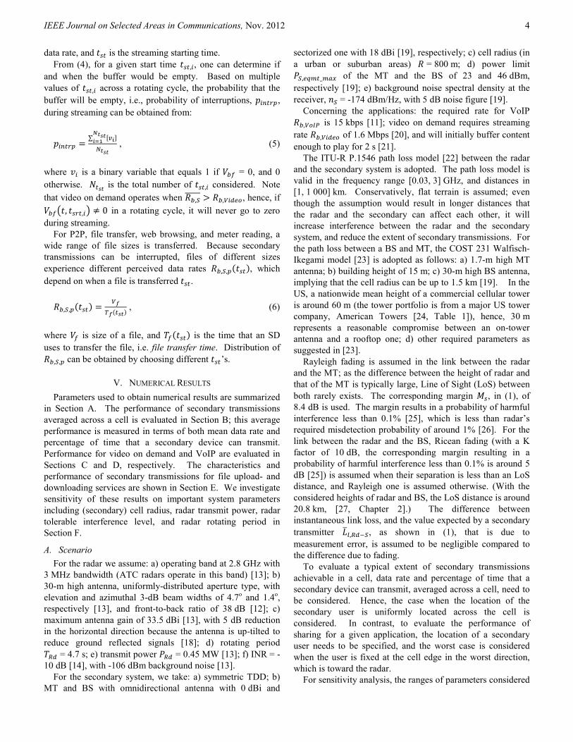
Fig. 6 shows the average secondary data rate, and the

percentage of time that an SD can transmit for both up- and

downstream, as a function of the cell radius. Fig. 6 shows

that, as expected, the average data rate and percentage of time

that a secondary device can transmit at a given distance from

the radar decreases with increasing cell radius. It is still the

case that extensive communications are possible for a cell that

is relatively close to the radar, but for larger cells, the cell

must be somewhat farther from the radar.

Fig. 6(a) shows that in the upstream, at 70 km from the

radar, the average data rate of a cell with 0.8 km radius is

around 60% of the system rate limit, as defined in Section V-

B; 70 km is around 24% of the 286 km distance. For a larger

cell, with 1.5 km radius, the same level of upstream data rate

can be achieved at around 100 km from the radar (35% of

286 km). Moreover, in the downstream, at only 14% of the

286 km distance, a cell with 1.5 km radius can achieve almost

100% of the system rate limit. Hence, the secondary system

can still achieve high data rates close to the radar, even with a

fairly large cell.

(a) Average Secondary Data Rate

0 10 20 30 40 50 60 700

2

4

6

8

10

12



1st Percentile

Mean

1 kB File

500 kB File

1 MB File

10 MB File

Mean

0.2 0.4 0.6 0.8 1 1.2 1.440

50

60

70

80

90

100

Cell Radius [km]

Average Data Rate [% of Data Rate in Dedicated Spectrum]

Upstream

Downstream

40 km from a Radar

20 km from a Radar

100 km from a Radar

70 km from a Radar


8

(b) Percentage of Time that a Secondary Device can Transmit

Figure 6 - Sensitivity of Extent of Transmissions on Cell Radius.

Fig. 7 shows the average data rate as a function of radar

transmit power. Changes in radar transmit power have a

similar effect on both data rate and the percentage of time that

an SD can transmit, similar to what we observed with changes

in cell radius in Fig. 6. Hence, results showing the percentage

of time that an SD can transmit are omitted for brevity.

Fig. 7 shows that the data rate decreases with increasing

transmit power of the radar. However, high average data rates

close to a radar can still be attained, even when the radar

transmit power is high, if the cell is a bit farther from the

radar. For example, in the upstream when the radar transmit

power increases from 0.5 to 1.4 MW, the distance from a cell

to the radar needs to be increased from around 70 to 90 km, so

that the achievable data rate is still around 60% of the system

rate limit (90 km is still only 31% of 286 km). In the

downstream, the increase in radar transmit power only slightly

decreases the average data rate, hence, the secondary system

can achieve high data rates at fairly short distance to a radar

transmitting with high power.

Figure 7 - Sensitivity of Average Data Rate on Radar Transmit Power.

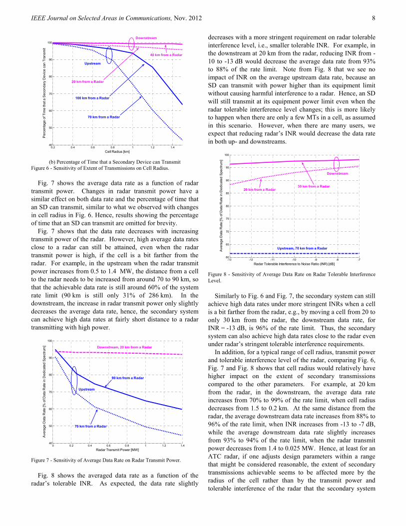
Fig. 8 shows the averaged data rate as a function of the

radar’s tolerable INR. As expected, the data rate slightly

decreases with a more stringent requirement on radar tolerable

interference level, i.e., smaller tolerable INR. For example, in

the downstream at 20 km from the radar, reducing INR from -

10 to -13 dB would decrease the average data rate from 93%

to 88% of the rate limit. Note from Fig. 8 that we see no

impact of INR on the average upstream data rate, because an

SD can transmit with power higher than its equipment limit

without causing harmful interference to a radar. Hence, an SD

will still transmit at its equipment power limit even when the

radar tolerable interference level changes; this is more likely

to happen when there are only a few MTs in a cell, as assumed

in this scenario. However, when there are many users, we

expect that reducing radar’s INR would decrease the data rate

in both up- and downstreams.

Figure 8 - Sensitivity of Average Data Rate on Radar Tolerable Interference

Level.

Similarly to Fig. 6 and Fig. 7, the secondary system can still

achieve high data rates under more stringent INRs when a cell

is a bit farther from the radar, e.g., by moving a cell from 20 to

only 30 km from the radar, the downstream data rate, for

INR = -13 dB, is 96% of the rate limit. Thus, the secondary

system can also achieve high data rates close to the radar even

under radar’s stringent tolerable interference requirements.

In addition, for a typical range of cell radius, transmit power

and tolerable interference level of the radar, comparing Fig. 6,

Fig. 7 and Fig. 8 shows that cell radius would relatively have

higher impact on the extent of secondary transmissions

compared to the other parameters. For example, at 20 km

from the radar, in the downstream, the average data rate

increases from 70% to 99% of the rate limit, when cell radius

decreases from 1.5 to 0.2 km. At the same distance from the

radar, the average downstream data rate increases from 88% to

96% of the rate limit, when INR increases from -13 to -7 dB,

while the average downstream data rate slightly increases

from 93% to 94% of the rate limit, when the radar transmit

power decreases from 1.4 to 0.025 MW. Hence, at least for an

ATC radar, if one adjusts design parameters within a range

that might be considered reasonable, the extent of secondary

transmissions achievable seems to be affected more by the

radius of the cell rather than by the transmit power and

tolerable interference of the radar that the secondary system

0.2 0.4 0.6 0.8 1 1.2 1.440

50

60

70

80

90

100

Cell Radius [km]

Percentage of Time that a Secondary Device can Transmit

Upstream

Downstream

40 km from a Radar

20 km from a Radar

100 km from a Radar

70 km from a Radar

0 0.2 0.4 0.6 0.8 1 1.2 1.440

50

60

70

80

90

100

Radar Transmit Power [MW]


Upstream

Downstream, 20 km from a Radar

90 km from a Radar

70 km from a Radar

-13 -12 -11 -10 -9 -8 -760

65

70

75

80

85

90

95

100

Radar Tolerable Interference to Noise Ratio (INR) [dB]


Downstream

Upstream, 70 km from a Radar

20 km from a Radar30 km from a Radar


9

will share spectrum with.

F-2 Sensitivity of Fluctuations in Perceived Secondary Data

Rate

Fig. 9 shows fluctuations in perceived data rate as a

function of file size: in the upstream at 70 km from the radar,

and in the downstream at 20 km. The fluctuations in

perceived data rate are evaluated for a user at the edge of a cell

in the direction toward the radar. It is seen, from Section V-E,

that when radar transmissions still affect transmissions of the

secondary system, the farther away from the radar, the higher

fluctuations in perceived data a secondary user would

experience. At 70 km from the radar for upstream and at

20 km for downstream, secondary transmissions are still

highly affected by the radar; Fig. 2 shows that the increasing

rate (i.e., slope) of the extent of secondary transmissions with

distance from the cell to the radar starts to decrease after

around 70 and 20 km for up- and downstreams, respectively.

Fig. 9(a) shows that, as expected, a user in a smaller cell

would experience higher fluctuations in perceived data rate

than that in a larger cell. However, the increase in fluctuations

in perceived data rate with decreasing cell radius will not be a

problem, as a user uploading large files (i.e., larger than

1 MB) would still experience insignificant fluctuations even

when the cell radius is as small as 200 m. For the

downstream, Fig. 9(b) shows that at only 20 km from the

radar, a user downloading large files would also experience

insignificant fluctuations in perceived data rate even when the

cell radius is 200 m. Hence, a user transferring a large file

would still experience insignificant fluctuations in perceived

data rate even in a small cell.

(a) Upstream

(b) Downstream

Figure 9 - Sensitivity of Perceived Secondary Data Rate on Secondary Cell

Radius.

The effect of the other parameters (including transmit

power, INR, and rotating period) on the fluctuations in

downstream perceived data rate are similar to the effect of cell

radius as shown in Fig. 9(b), hence, the results on fluctuations

of perceived data rate in the downstream are omitted. For the

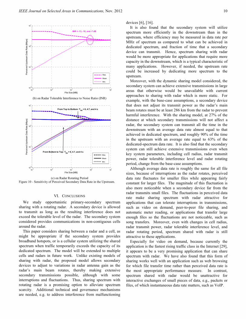
upstream, Fig. 10 shows the perceived data rate as a function

of file size when (a) the radar transmit powers are 0.025, 0.45,

and 1.4 MW, (b) INR is -13, -10, and -7 dB, and (c) the

rotating periods are 4, 4.7, and 6 s; the results are from a cell

70 km away from the radar. Fig. 10 shows that changes in

these three parameters have only marginal impact on the

fluctuations in data rate perceived when files larger than 1 MB

are uploaded. Hence, when one adjusts these parameters

within this reasonable range, a user transferring a large file

would still experience insignificant fluctuations in perceived

data rate. Note from Fig. 10(b) that, as we can expect from

the sensitivity analysis on average extent of secondary

transmissions, when a small number of users are assumed in a

cell, changing radar INR would have no impact on the

fluctuations in upstream perceived data rate.

(a) on Radar Transmit Power

10-3

10-2

10-1

100

101

10-2

10-1

100

101

102

File Size [MB]

Perceived Upstream Data Rate [Mbps]

Max.

Mean

Min. R = 0.2 km

R = 0.8 km

R = 1.5 km

10-3

10-2

10-1

100

101

10-1

100

101

102

File Size [MB]


Max.

Mean

Min.

R = 0.2, 0.8, and 1.5 km

10-3

10-2

10-1

100

101

10-2

10-1

100

101

File Size [MB]


Max.

Mean

Min.

PRd = 0.025 MW

PRd = 0.45 MW

PRd = 1.4 MW


10

(b) on Radar Tolerable Interference to Noise Ratio (INR)

(c) on Radar Rotating Period

Figure 10 - Sensitivity of Perceived Secondary Data Rate in the Upstream.

VI. CONCLUSIONS

We study opportunistic primary-secondary spectrum

sharing with a rotating radar. A secondary device is allowed

to transmit as long as the resulting interference does not

exceed the tolerable level of the radar. The secondary system

considered provides communications in non-contiguous cells

around the radar.

This paper considers sharing between a radar and a cell, as

might be appropriate if the secondary system provides

broadband hotspots, or is a cellular system utilizing the shared

spectrum when traffic temporarily exceeds the capacity of its

dedicated spectrum. The model will be extended to multiple

cells and radars in future work. Unlike existing models of

sharing with radar, the proposed model allows secondary

devices to adjust to variations in radar antenna gain as the

radar’s main beam rotates, thereby making extensive

secondary transmissions possible, although with some

interruptions and fluctuations. Thus, sharing spectrum with

rotating radar is a promising option to alleviate spectrum

scarcity. Additional technical and governance mechanisms

are needed, e.g. to address interference from malfunctioning

devices [6], [16].

It is also found that the secondary system will utilize

spectrum more efficiently in the downstream than in the

upstream, where efficiency may be measured in data rate per

MHz of spectrum as compared to what can be achieved in

dedicated spectrum, and fraction of time that a secondary

device can transmit. Hence, spectrum sharing with radar

would be more appropriate for applications that require more

capacity in the downstream, which is a typical characteristic of

many applications. However, if needed, the upstream rate

could be increased by dedicating more spectrum to the

upstream.

Moreover, with the dynamic sharing model considered, the

secondary system can achieve extensive transmissions in large

areas that otherwise would be unavailable with current

approaches to sharing with radar which is more static. For

example, with the base-case assumptions, a secondary device

that does not adjust its transmit power as the radar’s main

beam rotates must be at least 286 km from the radar to prevent

harmful interference. With the sharing model, at 27% of the

distance at which secondary transmissions will not affect a

radar, the secondary system can transmit all the time in the

downstream with an average data rate almost equal to that

achieved in dedicated spectrum, and roughly 90% of the time

in the upstream with an average rate equal to 63% of the

dedicated-spectrum data rate. It is also find that the secondary

system can still achieve extensive transmissions even when

key system parameters, including cell radius, radar transmit

power, radar tolerable interference level and radar rotating

period, change from the base-case assumptions.

Although average data rate is roughly the same for all file

sizes, because of interruptions as the radar rotates, perceived

data rate fluctuates for smaller files while appearing fairly

constant for larger files. The magnitude of this fluctuation is

also more noticeable when a secondary device far from the

radar transmits small files. The fluctuations in perceived data

rate make sharing spectrum with radar attractive for

applications that can tolerate interruptions in transmissions,

such as video on demand, peer-to-peer file sharing, and

automatic meter reading, or applications that transfer large

enough files so the fluctuations are not noticeable, such as

song transfers. Moreover, even with changes in cell radius,

radar transmit power, radar tolerable interference level, and

radar rotating period, spectrum shared with radar is still

attractive to these applications.

Especially for video on demand, because currently the

application is the fastest rising traffic class in the Internet [29],

it appears to be a very promising application that can share

spectrum with radar. We have also found that this form of

sharing works well with an application such as web browsing

for which file transfer time rather than perceived data rate is

the most appropriate performance measure. In contrast,

spectrum shared with radar would be unattractive for

interactive exchanges of small pieces of data, e.g., packets or

files, of which instantaneous data rate matters, such as VoIP.

10-3

10-2

10-1

100

101

10-2

10-1

100

101

File Size [MB]


Max.

Mean

Min.

INR = -13, -10, and -7 dB

10-3

10-2

10-1

100

101

10-2

10-1

100

101

File Size [MB]


Max.

Mean

Min.

From Bottom to Top: TRd = 6, 4.7, and 4 s

From Top to Bottom: TRd = 6, 4.7, and 4 s


11

ACKNOWLEDGMENT

The authors would like to thank Prof. Antonio A. Moreira,

of Instituto Superior Técnico, for very helpful discussions on

characteristics of radar and its antenna, and anonymous

reviewers for their insightful comments that help improving

the quality of this paper.

REFERENCES

[1] J.M. Peha, “Sharing spectrum through spectrum policy reform and

cognitive radio,” Proc. of the IEEE, vol.97, no.4, Apr. 2009, pp.708-19,

(www.ece.cmu.edu/~peha/wireless.html). [2] US National Telecommunications and Information Administration

(NTIA), Presentation: spectrum with significant federal commitments,

225 MHz - 3.7 GHz, 2009. [3] US NTIA, Federal Radar Spectrum Requirements, Special Publication

00-40, May 2000.

[4] R.P. Margie, “Efficiency, predictability, and the need for an improved interference standard at the FCC,” Proc. of 31st Telecommun. Policy

Research Conf. (TPRC), Arlington, VA, USA, Sep. 2003.

[5] US Federal Communications Commission (FCC), In the matter of Revision of Parts 2 and 15 of the Commission’s Rules to Permit

Unlicensed National Information Infrastructure (U-NII) devices in the 5

GHz band, MO&O, ET Docket No. 03-122, June 2006. [6] J.M. Peha, "Spectrum sharing in the gray space," to appear in

Telecommunication Policy Journal.

[7] R. Saruthirathanaworakun, and J.M. Peha, “Dynamic primary-secondary spectrum sharing with cellular systems,” Proc. of CrownCom, Cannes,

France, June 2010, (www.ece.cmu.edu/~peha/wireless.html).

[8] M.J. Marcus, “Sharing government spectrum with private users: opportunities and challenges,” IEEE Wireless Communications

Magazine, vol.16, no.3, June 2009, pp. 4-5.

[9] L. Wang, J. McGeehan, C. Williams, and A. Doufexi, “Radar spectrum opportunities for cognitive communications transmission,” Proc. of

CrownCom, Singapore, May 2008.

[10] M.I. Rahman, and J.S. Karlsson, “Feasibility evaluations for secondary LTE usage in 2.7-2.9 GHz radar bands,” Proc. of IEEE PIMRC,

Toronto, Canada, Sep. 2011.

[11] 3GPP, Technical Specification 22.105: Services and service capabilities, version 9.1.0, Release 9, Oct 2010.

[12] M.I. Skolnik, Introduction to Radar Systems, 3rd International Ed.,

McGraw-Hill, Singapore, 2001. [13] ITU-R, Rec. M.1464-1: Characteristics of radiolocation radars, and

characteristics and protection criteria for sharing studies for

aeronautical radionavigation and meteorological radars in the radiodetermination service operating in the frequency band 2 700-2 900

MHz, 2003. [14] B. Bedford and F. Sanders, “Spectrum sharing and potential interference

to radars,” Proc. of ISART, Boulder, CO, USA, Feb. 2007.

[15] UK Office of Communications (Ofcom), Coexistence of S Band radar systems and adjacent future services, Information Update, Dec. 2009.

[16] J.M. Peha, “Cellular systems and rotating radar using the same

spectrum,” Proc. of ISART, Boulder, CO, USA, July 2011, (www.ece.cmu.edu/~peha/wireless.html).

[17] N.M. Jacinto, Performance gains evaluation from UMTS/HSPA+ to LTE

at the radio network level, M.Sc. Thesis, IST-Tech. Univ. Lisbon, Portugal, 2009.

[18] R.L. Hinkle, R. M. Pratt, and R. J. Matheson, Spectrum Resource

Assessment in the 2.7 to 2.9 GHz Band Phase II: Measurements and Model Validation (Appendix A- Antenna Characteristic Modeling), OT

Report 76-97, Office of Telecommunications, US, Aug. 1976.

[19] H. Holma, P. Kinnunen, I.Z. Kovács, K. Pajukoski, K. Pedersen, and J. Reunanen, “Performance,” in H. Holma and A. Toskala (ed.), LTE for

UMTS: OFDMA and SC-FDMA Based Radio Access, John Wiley &

Sons, UK, 2009. [20] The Netflix Blog: (http://blog.netflix.com/2008/11/encoding-for-

streaming.html?CREATIVE=n&KID=k175726&USERID=618506686

&SESSIONID=id_618506687, June 2011). [21] A. Zambelli, IIS Smooth Streaming Technical Overview, White Paper,

Microsoft Cooperation, USA, 2009.

[22] ITU-R, Rec. P.1546-4: Method for point-to-area predictions for terrestrials services in the frequency range 30 MHz to 3 000 MHz, 2009.

[23] T. Kurner, “Propagation Model for Macro-Cells,” in E. Damosso, and

L.M. Correia (ed.), COST 231 Final Report, European Communities, Brussels, Belgium, 1999.

[24] R. Hallahan, and J.M. Peha, “Quatifying the cost of a nationawide public

safety wireless network,” Telecommunications Policy, vol.34, no.4, May 2010, pp. 200-20, (www.ece.cmu.edu/~peha/safety.html).

[25] ITU-R, Rec. P.1057-2: Probability distributions relevant to radiowave

propagation modeling, 2007. [26] J.T. Pinto, Assessment of multilateration telecommunication systems

installed in NAV, M.Sc. Thesis, IST-Tech. Univ. Lisbon, Portugal, 2011.

[27] J.D. Parsons, The Mobile Radio propagation Channel, 2nd Ed., John Wiley & Sons, Chichester, UK, 2000.

[28] S. Ramachandran, Web Metrics: Size and number of resources, Google,

(http://code.google.com/speed/articles/web-metrics.html, June 2011). [29] Cisco, Visual Networking Index: Global Mobile Data Traffic Forecast

Update, 2010–2015, White Paper, Cisco, USA, Feb. 2011.

Rathapon Saruthirathanaworakun (S’11) received the

B.Eng. and M.Eng degrees, both in electrical engineering, from Chulalongkorn University, Bangkok, Thailand.

Before pursuing Ph.D., he worked as an engineer for

TOT public limited company, formerly Telephone Organization of Thailand, and was responsible for

spectrum management and wireless engineering. Now, he

is a Ph.D. candidate in Engineering and Public Policy, in dual Ph.D. program between Carnegie Mellon University,

Pittsburgh, PA, USA, and Instituto Superior Técnico, Technical University of Lisbon, Portugal. His research topic is currently on spectrum management,

spectrum sharing model, and theirs implications on related regulation and

policy.

Jon M. Peha (S’, M’, SM’, F’11) received the B.Sc.

degree from Brown University, Providence, RI, and the Ph.D. degree in electrical engineering from Stanford

University, Stanford, CA.

He is a Full Professor at Carnegie Mellon University. He served in the US Government in 2008-2011, first as

Chief Technologist of the Federal Communications

Commission, and then Assistant Director of the White House Office of Science & Technology Policy where he

focused on Communications and Research. At Carnegie Mellon, he is a

Professor in the Dept. of Engineering & Public Policy and the Dept. of Electrical & Computer Engineering, and former Associate Director of the

university's Center for Wireless & Broadband Networking. He has served as

Chief Technical Officer for three high-tech companies, and a member of technical staff at SRI International, AT&T Bell Laboratories, and Microsoft.

He has addressed telecom and e-commerce policy on legislative staff in the

House Energy & Commerce Committee and the Senate, and helped launch and lead a US Government interagency program to assist developing countries

with information infrastructure. His research spans technical and policy issues

of information networks, including spectrum management, broadband Internet, wireless networks, video and voice over IP, communications for

emergency responders, universal service, secure Internet payment systems,

online dissemination of copyrighted material, and network security. He is an IEEE Fellow, an AAAS Fellow, and a winner of the FCC's "Excellence in

Engineering Award" and the IEEE TCCN Publication Award.

Luis M. Correia (S’85, M’91, SM’03) was born in

Portugal, on 1958. He received the Ph.D. in Electrical

and Computer Engineering from IST-TUL (Technical University of Lisbon) in 1991, where he is currently a

Professor in Telecommunications, with his work focused

in Wireless/Mobile Communications in the areas of propagation, channel characterisation, radio networks,

traffic, and applications. He has acted as a consultant for

Portuguese mobile communications operators and the telecommunications regulator, besides other public and private entities.

Besides being responsible for research projects at the national level, he has

been active in various ones within the European frameworks of RACE, ACTS, IST, ICT and COST (where he also served as evaluator and auditor),

having coordinated two COST projects, and taken leadership responsibilities

at various levels in many others. He has supervised more than 150 M.Sc. and Ph.D. students, having authored more than 300 papers in international and

national journals and conferences, for which he has served also as a reviewer,


12

editor, and board member, and edited 6 books. He was part of the COST

Domain Committee on ICT. He was the Chairman of the Technical Programme Committee of several conferences, namely PIMRC’2002. He is

part of the Expert Advisory Group and of the Steering Board of the European

Net!Works platform, and was the Chairman of its Working Group on Applications.

Documents

Opportunistic Sharing Single Radar and Cellularpeha/Opportunistic_Sharing__Single... · ATC radar (rotating horizontally with a constant speed), in a sharing scheme based only on