Dave Taliaferro OPTI 521 Optomechanical Engineering, Graduate Credit Tutorial

Integrated Opto-Mechanical Modeling :

Analyzing Wavefront Error due to Structural Vibration Introduction The multi-disciplinary nature of optical systems requires the use of disparate software tools to perform engineering analysis. These tools typically consist of CAD, finite-element analysis (FEA), math and simulation, optical design, and embedded control system firmware. Integrated Opto-Mechanical Modeling (IOMM) is the technique of combining these tools to effect system level design, performance analysis, and hardware implementation. Integration is achieved through the exchange of software results between tools. For dynamic analysis, data is exchanged between packages through operating system inter-process communication links such as shared memory. Most engineering software packages provide some standard link for the purposes of data exchange with other programs. This tutorial presents an application of IOMM to analyze a telescope’s exit pupil wavefront error (WFE) due to its structural vibrations. This analysis is “static”, in that no time sequencing or feedback loop is implemented in the simulation, but it does demonstrate some of the concepts for integrating theory and software to obtain useful results. For the vibration problem, telescope structure modal frequency information is obtained from the FEA, transformed to linear state-space representation in the mathematics and simulation software, which is transmitted to the optical design package through a dynamic data link to perform ray-trace OPD analysis. By scaling the vibration influence to the linear model so that the resultant WFE approaches 2 wavelengths of error, a sensitivity matrix relating motion of critical nodes to optical performance is derived.

Contents Introduction Tools used for this analysis Nastran Matlab\Simulink Zemax\Zelink Tutorial Problem : Wavefront Error due to Structural Vibration

Theoretical and Practical Relationships Relations of WFE. pupil coordinates, and equations of motion Linear Optical Modeling and State-Space Representation Nastran structure FEA modal frequency output Matlab nodal state-space representation

Zemax telescope optical prescription Analysis Procedure

Setting up a Simulink model to drive Zemax through Zelink Running the simulation

Results and Discussion References

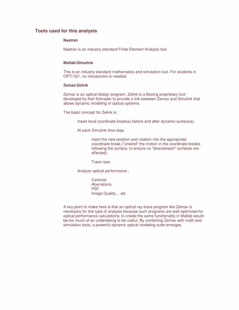
Tools used for this analysis Nastran Nastran is an industry standard Finite Element Analysis tool. Matlab\Simulink

This is an industry standard mathematics and simulation tool. For students in OPTI 521, no introduction is needed.

Zemax\Zelink

Zemax is an optical design program. Zelink is a Boeing proprietary tool developed by Karl Schrader to provide a link between Zemax and Simulink that allows dynamic modeling of optical systems. The basic concept for Zelink is :

Insert local coordinate break(s) before and after dynamic surface(s). At each Simulink time step:

inject the new position and rotation into the appropriate coordinate break ("unwind" the motion in the coordinate breaks following the surface, to ensure no "downstream" surfaces are affected).

Trace rays.

Analyze optical performance :

Centroid Aberrations PSF Image Quality… etc.

A key point to make here is that an optical ray-trace program like Zemax is necessary for this type of analysis because such programs are well-optimized for optical performance calculations; to create the same functionality in Matlab would be too much of an undertaking to be useful. By combining Zemax with math and simulation tools, a powerful dynamic optical modeling suite emerges.

Tutorial Problem : Wavefront Error due to Structural Vibration Space-borne telescopes will experience structural vibrations caused by motion slewing and reaction wheels, among other influences. These transient and steady–state disturbances will affect the optical system performance; therefore it is essential to determine the vibration frequency modes that have the greatest impact on WFE. To model these effects for a proposed space telescope, a primary mirror segment testbed has been constructed that contains piezo-electric actuators bonded to the backplane of the mirror segment. By changing the piezo actuator influence to mimic disturbance frequency modal shapes and measuring resultant WFE, information on which modes to minimize during structural design is obtained. Additionally, the mirror segment has been modeled in Nastran to provide disturbance simulations that produce mirror modal shapes based on structural disturbance frequencies. These modal shapes are transformed into linear state-space models in Matlab, which are then injected into the Zemax optical prescription for the telescope to obtain the WFE for each mode. There should be a numeric and visual correlation between the mode shapes and the wavefront map produced by Zemax. This tutorial presents an outline if that method, the goal of which is to develop sensitivity coeffecients for high-order wavefront aberrations caused by structural vibrations.

The sensitivity is defined as the derivative of WFE with respect to nodal position) times the change in nodal position :

( )yy

∆∂

∂ψ The WFE (ψ ) sensitivity due to changes in nodal positions.

Some additional definitions : Nodal : represents the physical system, the displacements and velocities of mirror physical nodes; the nodal model is a set of second order differential equations. Modal : defined as the displacements and velocities of structural modes; the shapes of the mirror when subjected to vibrations State-space : first-order representations of the nodal equations created by defining a state vector containing the nodal displacements and velocities; the first order representations express the inputs, outputs, and dynamics of the system in a form amenable to computation

Theoretical and Practical Relationships Relations of WFE. pupil coordinates, and equations of motion (note : Dr. Robert Fuentes wrote the following description, I am not recasting in terms of the linear model nomenclature for this assignment due to time constraints, so am providing it here to provide context for the subsequent discussions. See comment at end of this section.)

Nomenclature:

Symbol Definition q structural degree of freedom vector η modal degree of freedom vector

u input vector

w disturbance vector yx, x and y coordinates of the pupil

ψ wavefront error

Φ modal transformation matrix

B generalized force input matrix

D structural feedthrough correction matrix

Assume we have the following structural system:

wuB TT Φ+Φ=Λ++ ηηζη &&& , (1a)

uDq +Φ= η . (1b)

The wavefront error is a nonlinear function of the pupil (x,y) position and structural

degree of freedom

),,( qyxψψ = .

We wish to approximate the wavefront error in a Taylor expansion about the degree of

freedom vector. Let 0q denote the nominal degree of freedom vector about which we

will conduct a Taylor expansion. Then the nominal wavefront error can be “closely”

approximated in a ball ε<− 0qq , where 0>ε is sufficiently small, with

)(),,(),,(),,( 000 qqqyxq

qyxqyx −⋅∂

∂+≅

ψψψ . (2)

Substituting (1b) into (2) and assuming 00 =q , we have

( )uDyxq

yxqyx +Φ⋅∂

∂+≅ η

ψψψ )0,,()0,,(),,( . (3)

The contribution of the jth

degree of freedom to the sampled wavefront at pupil location

),( ii yx is )0,,( ii

j

yxq∂

∂ψ. Arranging the samples of wavefront ),,( qyx iii ψψ ≡ over the

pupil into vector form, [ ]iψψ ≡r

, we have the following vector relationship

( )uDq

q

q

+Φ

∂

∂+≅

=

ηψ

ψψ0

)0()(

rrv

. (4)

Let kΦr

be the kth

column of the modal matrix Φ and lDr

be the lth

column of the

feedthrough correction term D . Defining the following modal and input contributions to

the wavefront error,

k

k qΦ

∂

∂=

∂

∂ rrr

ψ

η

ψ,

l

l

Dqu

rrr

∂

∂=

∂

∂ ψψ,

the wavefront error is approximated as

∑∑== ∂

∂+

∂

∂+≅

m

l l

l

n

k k

ku

tuttq11

)()()0())((ψ

η

ψηψψ

rrrv

. (5)

Comment : For the next section describing the state-space representation;

uDq +Φ= η is redefined as : uDxCyrv

+=

Where C is the modal transformation matrix, and xv

is the modal degree of freedom

vector (the state vector).

For this analysis, we will obtain the state vector (containing structural node position and

velocity deltas) from the Nastran output, and will derive the C vector (the desired

sensitivities) by scaling the effects of the state vector and observing the resulting WFE.

Linear Optical Modeling and State-Space Representation From the optical system modal FEA information a state-space representation can be derived using Matlab. Among many other uses, this linear optical model lends itself conveniently to computer computation because of its matrix nature. An adequate description of state-space theory is beyond the scope of this assignment, see the references for more detail. Suffice to say that it is relatively easy to produce the stat-space model in Matlab. The system is described by :

uBxAxvr

& +=

uDxCyrv

+=

where the constant matrices

A = how the state evolves

B = the disturbances to the system; the piezo actuator influences

C = how the states affect the output; this is the sensitivity matrix we are

after

D = the direct feedthrough term

xv

= state vector ur

= disturbance input vector y = output

Repeating an earlier statement, we will obtain the state vector (containing structural node

position and velocity deltas) from the Nastran output, and will derive the C vector (the

desired sensitivities) by scaling the effects of the state vector and observing the resulting

WFE.

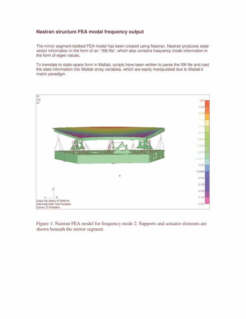
Nastran structure FEA modal frequency output The mirror segment testbed FEA model has been created using Nastran. Nastran produces state vector information in the form of an “.f06 file”, which also contains frequency mode information in the form of eigen values. To translate to state-space form in Matlab, scripts have been written to parse the f06 file and cast the state information into Matlab array variables, which are easily manipulated due to Matlab’s matrix paradigm.

XY

Z

0.27

0.239

0.208

0.177

0.146

0.115

0.0845

0.0536

0.0228

-0.00812

-0.039

-0.0699

-0.101

-0.132

-0.163

-0.193

-0.224

V1

L12

C1

Output Set: Mode 2 37.00406 Hz

Deformed(4.538): Total Translation

Contour: T3 Translation

Figure 1: Nastran FEA model for frequency mode 2. Supports and actuator elements are

shown beneath the mirror segment.

Matlab nodal state-space representation Using a Matlab script to read the Nastran f06 output file, a state vector is produced that contains the nodal positions and velocities relating to the frequency mode shapes.. For this analysis we are only interested in the positions. Each column in the state matrix represents a frequency mode. To perform the analysis, we simply pass each column into Zemax through the Zelink interface, and either observe the WFE map or store the values into an array. By adjusting the scaling of the state vector influences to a WFE of 2 wavelengths, the sensitivity values are obtained.

xv

=

⇓

⇑

velocityz

velocityy

velocityx

positionz

positiony

positionx

velocityz

velocityy

velocityx

positionz

positiony

positionx

nnode

nnode

nnode

nnode

nnode

nnode

MODE

node

node

node

node

node

node

1

1

1

1

1

1

1

velocityz

velocityy

velocityx

positionz

positiony

positionx

velocityz

velocityy

velocityx

positionz

positiony

positionx

nnode

nnode

nnode

nnode

nnode

nnode

MODE

node

node

node

node

node

node

⇓

⇑

2

1

1

1

1

1

1

…………

⇓

⇑

velocityz

velocityy

velocityx

positionz

positiony

positionx

velocityz

velocityy

velocityx

positionz

positiony

positionx

nnode

nnode

nnode

nnode

nnode

nnode

nMODE

node

node

node

node

node

node

1

1

1

1

1

1

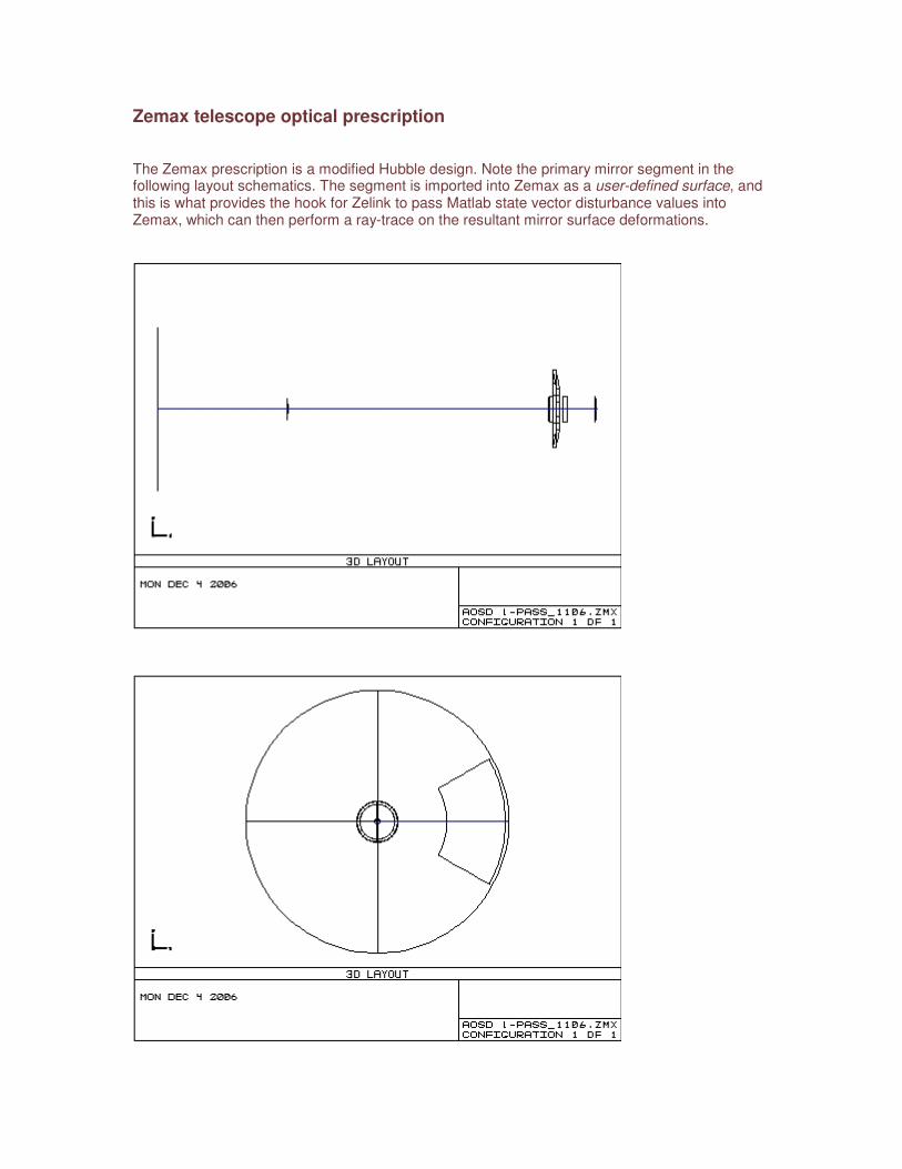
Zemax telescope optical prescription The Zemax prescription is a modified Hubble design. Note the primary mirror segment in the following layout schematics. The segment is imported into Zemax as a user-defined surface, and this is what provides the hook for Zelink to pass Matlab state vector disturbance values into Zemax, which can then perform a ray-trace on the resultant mirror surface deformations.

Analysis Procedure Procedure Outline :

From Nastran model,

Extract system modal information;

Convert to nodal representation (because zelink needs nodes in 6DOF)

Create state-space equation:

uBxAxvr

& +=

uDxCyrv

+=

Pass xv

vector to Zemax prescription through Zelink.

Analyze what happens to WFE due to xv

contributions.

Rescale xv

as necessary to get WFE to within 2 wavelengths.

Repeat for each frequency mode in the state matrix.

Setting up a Simulink model to drive Zemax through Zelink To perform the analysis, a Simulink model is created to obtain the state matrix values as a constant from the Matlab workspace. To make the connection between Matlab/Simulink and Zemax, the Zelink tool provides a Simulink library block which allows the user to tag the optical surface in the Zemax prescription for disturbance input.

Figure 4 : The Zelink Simulink library block dialog box showing surface 4 (the primary mirror segment) tagged for disturbance input.

Running the simulation Notice from Figure 5 the Simulink model setup. The state vector is passed to the Zemax prescription as a constant block, and Zemax calculates the new OPD (WFE) map from the resulting mirror surface deformations. To obtain the WFE due to the disturbances, the reference OPD (the unaberrated OPD from an undisturbed system) is subtracted from the Zemax output. The simulation can be run from the Matlab workspace prompt or by clicking the run button in Simulink. To estimate the gain value for scaling the input, the y translation information is obtained from the state matrix. The following plot show the relative magnitude of the y translation :

Figure 5 : Y axis translation for the nodal degrees of freedom, refer to script next page

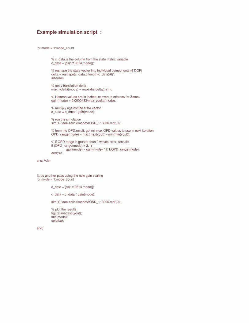
Example simulation script : for mode = 1:mode_count % c_data is the column from the state matrix variable c_data = [cs(1:10614,mode)]; % reshape the state vector into individual components (6 DOF) delta = reshape(c_data,6,length(c_data)/6)'; size(del) % get y translation delta max_ydelta(mode) = max(abs(delta(:,2))); % Nastran values are in inches; convert to microns for Zemax gain(mode) = 0.0000433/max_ydelta(mode); % multiply against the state vector c_data = c_data * gain(mode); % run the simulation sim('C:\aaa-zelink\mode\AOSD_113006.mdl',0); % from the OPD result, get minmax OPD values to use in next iteration OPD_range(mode) = max(max(yout)) - min(min(yout)); % if OPD range is greater than 2 waves error, rescale if (OPD_range(mode) > 2.1) gain(mode) = gain(mode) * 2.1/OPD_range(mode); end;%if end; %for % do another pass using the new gain scaling for mode = 1:mode_count c_data = [cs(1:10614,mode)]; c_data = c_data * gain(mode); sim('C:\aaa-zelink\mode\AOSD_113006.mdl',0); % plot the results figure;imagesc(yout); title(mode); colorbar; end;

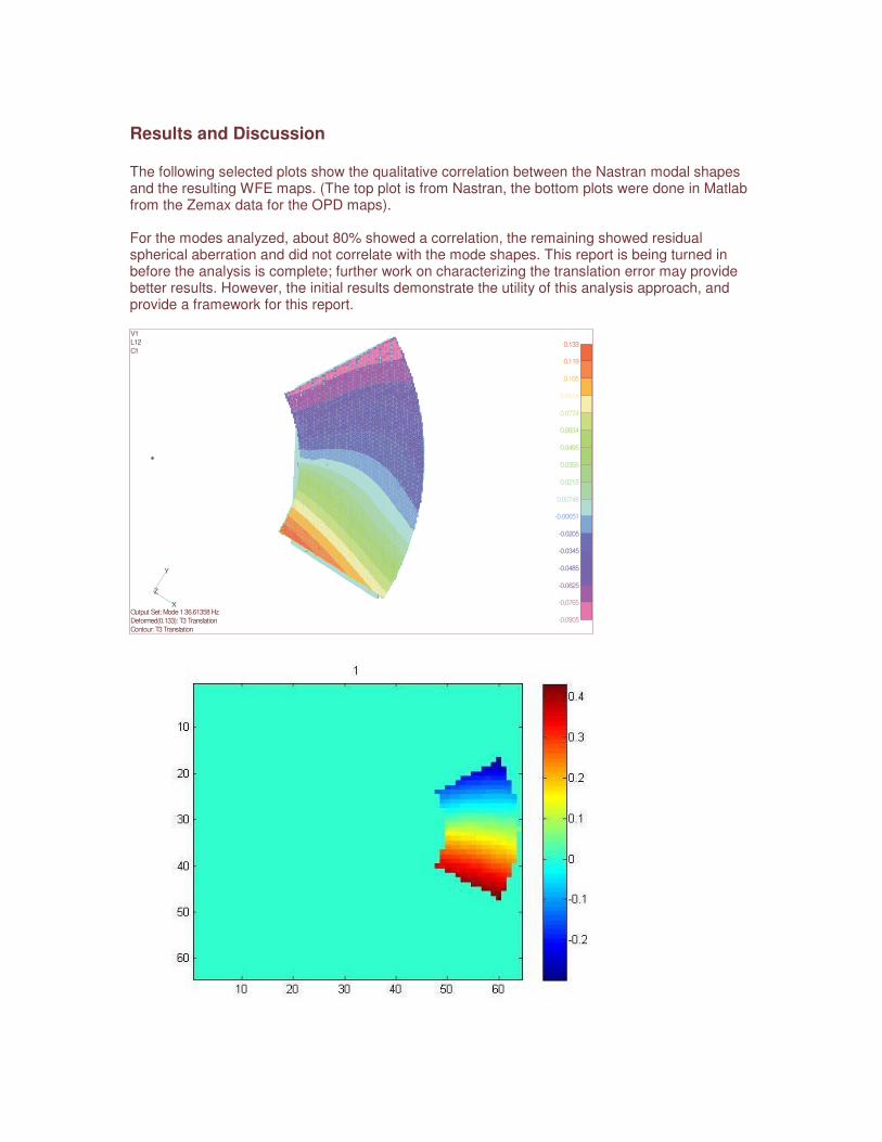
Results and Discussion The following selected plots show the qualitative correlation between the Nastran modal shapes and the resulting WFE maps. (The top plot is from Nastran, the bottom plots were done in Matlab from the Zemax data for the OPD maps). For the modes analyzed, about 80% showed a correlation, the remaining showed residual spherical aberration and did not correlate with the mode shapes. This report is being turned in before the analysis is complete; further work on characterizing the translation error may provide better results. However, the initial results demonstrate the utility of this analysis approach, and provide a framework for this report.

X

Y

Z

0.133

0.119

0.105

0.0914

0.0774

0.0634

0.0495

0.0355

0.0215

0.00748

-0.00651

-0.0205

-0.0345

-0.0485

-0.0625

-0.0765

-0.0905

V1

L12

C1

Output Set: Mode 1 36.61358 Hz

Deformed(0.133): T3 Translation

Contour: T3 Translation

X

Y

Z

0.27

0.239

0.208

0.177

0.146

0.115

0.0845

0.0536

0.0228

-0.00812

-0.039

-0.0699

-0.101

-0.132

-0.163

-0.193

-0.224

V1

L12

C1

Output Set: Mode 2 37.00406 Hz

Deformed(0.27): T3 Translation

Contour: T3 Translation

X

Y

Z

0.0372

0.0325

0.0279

0.0232

0.0186

0.0139

0.00929

0.00464

-0.0000106

-0.00466

-0.00931

-0.014

-0.0186

-0.0233

-0.0279

-0.0326

-0.0372

V1

L12

C1

Output Set: Mode 11 107.8424 Hz

Deformed(0.0372): T3 Translation

Contour: T3 Translation

References Books (look on Amazon.com for information) : Theory of Matrix Structural Analysis, by J. S. Przemieniecki Introduction to Dynamics and Control of Flexible Structures, by John L. Junkins, Youdan Kim Integrated Optomechanical Analysis, by Keith Doyle, Victor Genberg, Gregory Michels, http://www.sigmadyne.com/sigweb/pubs.htm Linear Optical Modeling : Steve Griffin, Karl Schrader, Boeing-SVS, Modeling Dynamic Optical Systems, SPIE tutorial with some limited discussion of Zelink. Karl Schrader is the creator of Zelink. Redding, D., Breckinridge, W., Optical Modeling for Dynamics and Control Analysis, 1991; Guidance, Navigation and Control Conference, Portland, OR, 1990 Technical Papers, American Institute of Aeronautics and Astronautics Redding, D., Millman, M., Loboda, G. Linear Analysis of Opto-Mechanical Systems, Proceedings of SPIE -- Volume 1696 Controls for Optical Systems, July 1992, Angeli, G., Gregory, B., Linear optical model for a large ground-based telescope, Proceedings of SPIE --

Volume 5178, Optical Modeling and Performance Predictions, Mark A. Kahan, Editor, January 2004, Howard, J., Optical modeling activities for the James Webb Space Telescope (JWST) project: I. The linear optical model, Proceedings of SPIE -- Volume 5178 Optical Modeling and Performance Predictions, Mark A. Kahan, Editor, January 2004, Integrated Optical Modeling : Miller, D., deWeck, O., Framework for Multidisciplinary Integrated Modeling and Analysis of Space Telescopes, Proceedings of SPIE -- Volume 4757 Integrated Modeling of Telescopes, July 2002 Miller, D., deWeck, O., Integrated modeling and dynamics simulation for the Next Generation Space Telescope (NGST), Proceedings of SPIE -- Volume 4013 UV, Optical, and IR Space Telescopes and Instruments, July 2000 Angeli, G., et al, Modeling tools to estimate the performance of the Thirty Meter Telescope: an integrated approach, Proceedings of SPIE -- Volume 5497 Modeling and Systems Engineering for Astronomy, September 2004, pp. 237-250 Mosier, G., Howard, J., et al , The role of integrated modeling in the design and verification of the James

Webb Space Telescope, Proceedings of SPIE -- Volume 5528 Space Systems Engineering and Optical

Alignment Mechanisms, September 2004

Howard, J., Ha, K., Optical modeling activities for the James Webb Space Telescope (JWST) project: II. Determining image motion and wavefront error over an extended field of view with a segmented optical system, Proceedings of SPIE -- Volume 5487 Optical, Infrared, and Millimeter Space Telescopes, October 2004 Mosier, G., Howard, J., et al, Integrated modeling activities for the James Webb Space Telescope:

structural-thermal-optical analysis, Proceedings of SPIE -- Volume 5487

Optical, Infrared, and Millimeter Space Telescopes, October 2004

Mosier, G., Howard, J., et al, Integrated modeling activities for the James Webb Space Telescope: optical jitter analysis, Proceedings of SPIE -- Volume 5487 Optical, Infrared, and Millimeter Space Telescopes, October 2004 Schipani, P., Perrotta, F., Marty, L., Integrated modeling approach for an active optics system, Proceedings

of SPIE -- Volume 6271 Modeling, Systems Engineering, and Project Management for Astronomy II,

627116 (Jun. 23, 2006) Mosier, Redding, et al, NGST Performance Analysis Using Integrated Modeling, NGST Project Study Office, Goddard Space Flight Center, 2000 Hatheway, A., Error Budgets for Optomechanical Modeling, Proc SPIE, Vol, 5178 Roberts, S., et al, Integrated modeling of the Canadian Very Large Telescope, National Research Council Canada Wavefront Analysis Redding , D., Sigrist , N., Lou, J., Zhang, Y. Optical State Estimation Using Wavefront Data, Proceedings

of SPIE -- Volume 5523 Current Developments in Lens Design and Optical Engineering V, October 2004

Redding , D., Sigrist , N., Lou, J., Zhang, Y. , Optical system alignment via optical state estimation using

wavefront measurements, Proceedings of SPIE -- Volume 5965

Optical Fabrication, Testing, and Metrology II, (Oct. 19, 2005)

Ohara,C., Redding, D., PSF monitoring and in-focus wavefront control for NGST, Proceedings of SPIE --

Volume 4850 IR Space Telescopes and Instruments, March 2003

Phase Diversity

These sites have good theory and links to phase diversity papers http://waf.eps.hw.ac.uk/index.htm http://www.optics.rochester.edu/workgroups/fienup/Publications.htm Jeffries, S., et al, Sensing wave-front amplitude and phase with phase diversity, Journal OSA, 2002 Carrara, D., Thelen, B., Paxman, R., Aberration correction of segmented-aperture telescopes by using phase diversity, Proceedings of SPIE -- Volume 4123

Image Reconstruction from Incomplete Data, Michael A. Fiddy, Rick P. Millane, Editors, November 2000, pp. 56-63 Paxman, R., Fienup, J., Optical misalignment sensing and image reconstruction using phase diversity, J.Opt.Soc.Am.A/Vol.5,No.6, June 1988 Tyler, D., et al, Comparison of image reconstruction algorithms using adaptive optics instrumentation, Proceedings of SPIE -- Volume 3353 Adaptive Optical System Technologies, September 1998, pp. 160-171 Zernike Riera, P., Computation of the circle polynomials of Zernike, Proceedings of SPIE -- Volume 5162

Advanced Wavefront Control: Methods, Devices, and Applications, December 2003, Wang, J., Silva, D., Wave-front interpretation with Zernike polynomials, Applied Optics, Vol19, No.9, 1980 Piezoelectrics Good tutorial : http://www.physikinstrumente.com/en/products/piezo_tutorial.php State-space Systems : Good state-space tutorials : http://cnx.org/content/col10143/1.3 http://www.duke.edu/~hpgavin/ce131/ Dietz, S., et al, Nodal vs. Modal Representation in Flexible Multibody System Dynamics. Multibody Dynamics, 2003