Embed Size (px)
Citation preview

DOCTOR OF PHILOSOPHY
Optical characterisation of a low temperature plasma jet
Irwin, Rachael
Award date:2020
Awarding institution:Queen's University Belfast
Link to publication
Terms of useAll those accessing thesis content in Queen’s University Belfast Research Portal are subject to the following terms and conditions of use
• Copyright is subject to the Copyright, Designs and Patent Act 1988, or as modified by any successor legislation • Copyright and moral rights for thesis content are retained by the author and/or other copyright owners • A copy of a thesis may be downloaded for personal non-commercial research/study without the need for permission or charge • Distribution or reproduction of thesis content in any format is not permitted without the permission of the copyright holder • When citing this work, full bibliographic details should be supplied, including the author, title, awarding institution and date of thesis
Take down policyA thesis can be removed from the Research Portal if there has been a breach of copyright, or a similarly robust reason.If you believe this document breaches copyright, or there is sufficient cause to take down, please contact us, citing details. Email:[email protected]
Supplementary materialsWhere possible, we endeavour to provide supplementary materials to theses. This may include video, audio and other types of files. Weendeavour to capture all content and upload as part of the Pure record for each thesis.Note, it may not be possible in all instances to convert analogue formats to usable digital formats for some supplementary materials. Weexercise best efforts on our behalf and, in such instances, encourage the individual to consult the physical thesis for further information.
Download date: 26. Mar. 2022

Optical Characterisation of a Low
Temperature Plasma Jet
by
Rachael Irwin
MSci
A thesis presented upon application for
admission to the degree of Doctor of Philosophy
School of Mathematics & Physics
Queen’s University Belfast
April 2020

i
AcknowledgementsFirstly, I would like to thank my supervisor, Professor David Riley, for giv-
ing me the opportunity to study for a PhD and for his support throughout.
Without his help and guidance it would not have been possible. Also a mas-
sive thank you to my second supervisor Professor Bill Graham, whose insight
and knowledge throughout was very much appreciated.
I would like to thank my post doc, Dr Steven White, who taught me so
much and for all his help and constant support, especially in the lab. I am also
very grateful to the workshop team for all the work that they do, without them
these experiments would not be possible. Also a thank you to Dr Gagik Ner-
sisyan whose knowledge and help over the last few years has been invaluable.
The financial support from EPSRC is also gratefully acknowledged.
A huge thank you to all my friends and colleagues at QUB. There are too
many of you to thank individually, but I’m glad I decided to do a PhD because
of all the great friends I’ve made along the way.
A massive thank you to Hannah for all your support (we made it!), for all
the coffee breaks, drinks and ’write, whine and wine’ nights that helped me
through it all. Also a special mention to my ’physics Auntie’ Emma, whose
chats and catch ups about anything other than Physics kept me sane.
Thank you to Dave Bailie, my fellow Liverpool fan, who kept me sane on
RAL experiments and to Tom Hodge who was a massive source of support,
especially during the write up stage.
Thank you to all the clerical staff in the department, but a special mention
to Teresa and Jillian who do so much that goes unnoticed.
And thank you to Parlour, those Friday night pints made everything more
bearable.

ii
Finally, I would like to thank my family for supporting and helping me
through some of the toughest years of my life. It wouldn’t have been possible
without you.
I’ll always remember 2020 as the year I finally finished my PhD... and the
year Liverpool finally won the league! (Had to get it in somewhere).

iii
AbstractLow temperature plasma jets are of particular interest due to their unique way
of producing reactive species even at room temperature and atmospheric pres-
sure. They therefore have the potential to be used for various applications, in
plasma medicine and surface modification in particular. The characterisation
of these plasma jets is important in order to be able to control them for the
desired application.
Various optical diagnostics have been implemented to establish the forma-
tion and propagation of the plasma, as well as to estimate the important pa-
rameters such as electron density, ne, and electron temperature, Te. Initially
imaging on nanosecond timescale established that the plasma, although con-
tinuous to the naked eye, consisted of plasma bullets travelling at velocities of
up to 105 m s−1. 2D quasi monchromatic images of the plasma, obtained by
isolating the light produced by individual spectral transitions, allowed an esti-
mation of the density of excited helium states within the plasma, in the region
of 1× 10⁹ − 2× 1010 cm−3.
Optical emission spectroscopy was used to identify the species present, to
estimate the electron temperature of the plasma using helium line ratios, and
to estimate the gas temperature using nitrogen emission. The electron tem-
perature and gas temperature were found to be 0.3 eV and 303 K respectively,
which confirmed that the plasma jet was operating in the low temperature
regime. Emission from allowed and forbidden helium lines was also utilised,
in this case to estimate the electric field present, which was calculated to be
32.1 kV cm−1.
Thomson scattering was also attempted in an effort to obtain electron den-
sity and temperature estimates. However, the electron density of the plasma in

iv
question was simply too low to detect using the experimental set-up at hand.
However, using a model consisting of data from Raman scattering it was pos-
sible to put an upper limit on the electron density of the plasma of 9.95× 10¹²
cm−3.

v
Contents
Acknowledgements i
Abstract iii
1 Introduction 1
1.1 Plasma . . . . . . . . . . . . . . . . . . . . . . . . . . . . . . . . . 1
1.1.1 Plasma criteria . . . . . . . . . . . . . . . . . . . . . . . . 1
1.2 Thermal and non-thermal plasmas . . . . . . . . . . . . . . . . . 3
1.2.1 Low temperature atmospheric pressure plasmas . . . . . 4
1.3 Motivation . . . . . . . . . . . . . . . . . . . . . . . . . . . . . . . 5
1.3.1 Applications . . . . . . . . . . . . . . . . . . . . . . . . . . 5
1.3.2 Work at QUB . . . . . . . . . . . . . . . . . . . . . . . . . 7
1.4 Formation of the plasma . . . . . . . . . . . . . . . . . . . . . . . 8
1.4.1 Townsend mechanism . . . . . . . . . . . . . . . . . . . . 8
1.4.2 Streamer mechanism . . . . . . . . . . . . . . . . . . . . . 11
1.4.3 Dawson photo-ionisation theory . . . . . . . . . . . . . . 13
1.4.4 Ionisation wave propagation theory . . . . . . . . . . . . 15
1.5 Thomson scattering . . . . . . . . . . . . . . . . . . . . . . . . . . 16
1.5.1 Laser-plasma interaction . . . . . . . . . . . . . . . . . . . 16
1.5.2 Rayleigh and Raman scattering . . . . . . . . . . . . . . . 19
1.6 Objectives . . . . . . . . . . . . . . . . . . . . . . . . . . . . . . . 21

vi
1.7 Thesis outline . . . . . . . . . . . . . . . . . . . . . . . . . . . . . 21
2 Experimental Set-up and Diagnostics 23
2.1 Plasma jet . . . . . . . . . . . . . . . . . . . . . . . . . . . . . . . 24
2.1.1 Helium gas flow . . . . . . . . . . . . . . . . . . . . . . . 26
2.2 Imaging . . . . . . . . . . . . . . . . . . . . . . . . . . . . . . . . 29
2.3 Optical emission spectroscopy (OES) . . . . . . . . . . . . . . . . 33
2.4 Thomson scattering set-up . . . . . . . . . . . . . . . . . . . . . . 35
2.4.1 Probe laser . . . . . . . . . . . . . . . . . . . . . . . . . . . 36
2.4.2 Double grating spectrometer . . . . . . . . . . . . . . . . 37
2.4.3 Plasma jet and laser alignment . . . . . . . . . . . . . . . 38
3 Plasma Jet Imaging 44
3.1 Plasma imaging . . . . . . . . . . . . . . . . . . . . . . . . . . . . 45
3.1.1 Experimental set-up . . . . . . . . . . . . . . . . . . . . . 47
3.2 Plasma bullet imaging results . . . . . . . . . . . . . . . . . . . . 49
3.2.1 Bullet velocity - horizontal jet orientation . . . . . . . . . 50
3.2.2 Bullet velocity - vertical jet orientation
(downwards propagation) . . . . . . . . . . . . . . . . . . 55
3.2.3 Bullet size . . . . . . . . . . . . . . . . . . . . . . . . . . . 58
3.2.4 Bullet velocity dependence on gas flow . . . . . . . . . . 60
3.3 2D quasi monochromatic imaging . . . . . . . . . . . . . . . . . 62
3.3.1 2D imaging data . . . . . . . . . . . . . . . . . . . . . . . 63
3.3.2 Data analysis method - Abel inversion . . . . . . . . . . . 66
3.3.3 2D imaging - Data analysis . . . . . . . . . . . . . . . . . 69
3.4 Summary . . . . . . . . . . . . . . . . . . . . . . . . . . . . . . . . 78

vii
4 Emission Spectroscopy 79
4.1 Experimental set-up . . . . . . . . . . . . . . . . . . . . . . . . . 80
4.2 Emission spectra data collection . . . . . . . . . . . . . . . . . . . 81
4.2.1 Spectra between electrodes . . . . . . . . . . . . . . . . . 81
4.2.2 Spectra from the plasma plume . . . . . . . . . . . . . . . 84
4.3 Electron temperature estimates using line ratios . . . . . . . . . 87
4.3.1 Local thermodynamic equilibrium (LTE) . . . . . . . . . 87
4.3.2 Electron temperature calculation . . . . . . . . . . . . . . 90
4.3.3 Other results using electron temperature . . . . . . . . . 95
4.4 Nitrogen spectra and gas temperature . . . . . . . . . . . . . . . 97
4.5 Helium emission spectra at 447nm and 492nm . . . . . . . . . . 99
4.5.1 447nm results . . . . . . . . . . . . . . . . . . . . . . . . . 106
4.5.2 492nm results . . . . . . . . . . . . . . . . . . . . . . . . . 107
4.6 Summary . . . . . . . . . . . . . . . . . . . . . . . . . . . . . . . . 110
5 Thomson Scattering 112
5.1 Initial set-up . . . . . . . . . . . . . . . . . . . . . . . . . . . . . . 113
5.2 Synchronisation . . . . . . . . . . . . . . . . . . . . . . . . . . . . 115
5.2.1 Triggering system . . . . . . . . . . . . . . . . . . . . . . . 115
5.2.2 Internal timing . . . . . . . . . . . . . . . . . . . . . . . . 117
5.3 Results . . . . . . . . . . . . . . . . . . . . . . . . . . . . . . . . . 119
5.3.1 Rayleigh scattering . . . . . . . . . . . . . . . . . . . . . . 119
5.3.2 Raman scattering . . . . . . . . . . . . . . . . . . . . . . . 120
5.3.3 Thomson scattering . . . . . . . . . . . . . . . . . . . . . . 125
5.4 Data analysis method - Raman model . . . . . . . . . . . . . . . 135
5.4.1 Raman model . . . . . . . . . . . . . . . . . . . . . . . . . 135
5.4.2 Results from model . . . . . . . . . . . . . . . . . . . . . . 137

viii
5.4.3 Electron density detection limit . . . . . . . . . . . . . . . 139
5.5 Summary . . . . . . . . . . . . . . . . . . . . . . . . . . . . . . . . 141
6 Conclusions and Future Work 142
6.1 Conclusions . . . . . . . . . . . . . . . . . . . . . . . . . . . . . . 143
6.2 Future work . . . . . . . . . . . . . . . . . . . . . . . . . . . . . . 146
A Other Work 149
B Publications related to other work 150
Bibliography 151

1
Chapter 1
Introduction
1.1 Plasma
Plasma is regarded as the fourth state of matter which occurs when a gas is
heated and sufficiently ionised. It makes up 97 % of the universe [1] and was
a term first used by Langmuir in 1928 [2] to describe a region of free elec-
trons and positive ions not influenced by its boundaries, discovered in an arc
discharge. The zone between the plasma and its boundaries is known as the
plasma sheath region [3].
1.1.1 Plasma criteria
A plasma is the accumulation of free electrons and positive ions, which occurs
when a gas is heated and sufficiently ionised. To be defined as a plasma, the
Debye length, λD, must be smaller than the length of the system, λD L. The
Debye length is the distance over which the potential of a charge is shielded
from externally applied fields due to the mobility of the electrons and ions in
response to the local field, and is a function of the electron density, ne, and the
electron temperature, Te. It is given by:

Chapter 1. Introduction 2
λD = (ε0 kB Te
ne e2 )12 (1.1)
where ε0 is the permittivity of free space, kB is Boltzmann’s constant and e is
the electron charge. This also implies quasi-neutrality, as the plasma is free
from large electric fields and can be considered neutral where ni ' ne ' n,
where ni is the ion density, ne is the electron density and n is the plasma den-
sity. This means that the plasma as a whole is neutral, however locally there
may be a charge imbalance [4].
The plasma will exhibit collective behaviour, but only if the charge density
is sufficiently high. The plasma parameter, ND, defines the number of free
electrons in the Debye sphere, which is the volume with a radius equal to the
debye length. ND must be much greater than 1, where ND = 43 πneλ
3D.
The plasma frequency, ωp, must also be considered. This is the lowest fre-
quency at which an electromagnetic wave can propagate through the plasma
[5]. It is defined as:
ωp = (ne e2
me ε0)
12 (1.2)
If τ is the mean time between collisions within the plasma then ωτ > 1 must
be true for the ionised gas to behave as a plasma [6].
Throughout this work, the electron temperature of the plasma will be ex-
pressed in electron volts (eV), where 1 eV = 11,600 K. The average kinetic en-
ergy of particles in the plasma can be given by:
E =32
kBT (1.3)
where kB is the Boltzmann’s constant in J/K and T is the temperature in Kelvin.

Chapter 1. Introduction 3
Hence kBT is in units of Joules and kBT = 1 eV when T = 11, 600 K. This
assumes a Maxwellian distribution of the particles in the plasma.
1.2 Thermal and non-thermal plasmas
A thermal plasma can be described by one temperature, i.e. T = Te = Ti = Tg,
where Te is the electron temperature, Ti is the ion temperature and Tg is the gas
temperature. This is due to all of the constituents of the plasma, electrons, ions
and gas particles, being in thermodynamic equilibrium. Thermal plasmas are
capable of delivering high power at high pressures and are therefore used in
applications such as fusion plasma, welding and cutting [7, 8]. However, the
applications of thermal plasmas are limited in some areas such as medicine,
due to their exceptionally high gas temperature and low excitation selectivity
[7]. This has led to an increase in interest in non-thermal plasmas in recent
time.
Non-thermal, or low temperature, plasmas are not in thermodynamic equi-
librium and hence do not display a consistent temperature across the con-
stituents of the plasma. The energy in the system generates energetic electrons
but due to the inefficient transfer of energy to the heavier particles, the gas re-
mains at a much lower temperature i.e. Te Tg. They can offer high energy
efficiency in chemical reactions due to the production of excited species, such
as free radicals, while operating at low temperatures [7, 8]. This chemically
rich environment operating at room temperature has led to the possibility of
many applications concerning temperature sensitive materials.

Chapter 1. Introduction 4
1.2.1 Low temperature atmospheric pressure plasmas
Figure 1.1 shows types of atmospheric pressure discharges ranging from low
density, Townsend discharges to arc discharges more than 10 orders of magni-
tude greater in electron density.
FIGURE 1.1: Types of atmospheric pressure dischargesdepending on gas temperature and electron density (T.D.represents Townsend Discharge) [9].
A low temperature plasma in this case refers to one with a gas temperature
around room temperature and an electron temperature up to a few eV.
A plasma at atmospheric pressure is harder to maintain than at low pres-
sure as any heating of the gas can lead to arcing and hence a thermal plasma
is created. Several approaches have been investigated to achieve a low tem-
perature plasma at atmospheric pressure. One is a dielectric barrier discharge
(DBD) which consists of two parallel metal electrodes which are covered in a

Chapter 1. Introduction 5
dielectric coating. This prevents arcing of the plasma as the dielectric layer
limits the current in the plasma [10].
Another possible method of sustaining a low temperature plasma at atmo-
spheric pressure is using nanosecond pulsed plasmas as the discharge will not
last long enough for arcing to occur.
Micro plasmas are also beneficial as their small size, a few µm to 1 mm,
means the energy lost by the discharge to the surroundings is large compared
to the size of the plasma [10].
The majority of methods to create low temperature plasmas restrict the
plasma to the area between the electrodes which limits the number of possible
applications. However, to overcome this there has been research into the use
of atmospheric pressure plasma jets (APPJ’s), a method which still creates the
plasma between two electrodes, however a gas flows through the tube where
the plasma is created allowing it to propagate out into ambient air, creating a
plasma plume or "plasma pencil" as it is sometimes known. This allows the
reactive species produced in the plasma to be used in a wider variety of appli-
cations. By controlling the applied voltage across the electrodes, the driving
frequency and the gas flow velocity, arcing can be avoided [3]. In this thesis an
APPJ sustained using helium gas flow will be investigated.
1.3 Motivation
1.3.1 Applications
An important factor regarding low temperature plasmas is that they can pro-
duce reactive species capable of initiating reactions, even at these low tempera-
tures, that are difficult to obtain otherwise [3]. This has led to a great interest in

Chapter 1. Introduction 6
low temperature plasmas in biomedicine, material science and the fabrication
industry.
The use of plasmas in medicine is not a new concept, as they have been
used previously for applications such as tissue cutting and coagulation. An
example of such a device is an Argon Plasma Coagulator (APC) described by
Robotis et al. [11]. However, these devices achieve a biological response using
thermal effects, where as low temperature plasmas are capable of obtaining
such a response by the production of reactive oxygen and nitrogen species
(RONS), or through strong electric fields [12]. It is hoped that this production
of RONS could lead to improved cancer therapy. Therapies such as radiother-
apy only produce reactive oxygen species (ROS), however the production of
NO by a low temperature plasma could induce apoptosis, halting the genera-
tion of cancer cells and therefore improving cancer therapy [13–15].
These plasmas are still not well understood, but the plethora of possible
applications as well as the emergence of the plasma medicine field has acceler-
ated research in recent years [16]. The emergence of these possible applications
led to the need for low temperature plasma jets, a source which was capable
of propagating the plasma into ambient air. Understanding the characteristics
of these plasmas is crucial in order to control them for the desired application,
as in the case of biomedical applications it is essential that the electron temper-
ature is sufficiently high to activate the biochemistry, but the gas temperature
remains low enough for direct contact with human skin, typically < 40C [14,
16]. This allows specific cells to be targeted while not affecting the healthy
cells. Another important aspect of low temperature plasmas is that they oper-
ate at room temperature and pressure and hence the necessity for a vacuum is
Chapter 1. Introduction 7
removed, meaning they are a cost effective option for a wide range of applica-
tions in medicine and healthcare.
Within the field of plasma medicine there have already been numerous in-
vestigations into the possibility of using low temperature plasmas for applica-
tions such as; surface and surgical equipment sterilisation [14, 17–20], wound
healing and sterilisation [18, 20–25], dental treatment [18, 23], bacterial inacti-
vation [26, 27], cancer treatment [23, 24, 28], DNA damage [29] and many other
biomedical applications [30].
Outside of plasma medicine other applications using low temperature plas-
mas include the surface modification of materials [19, 31, 32], nano-structure
fabrication [33], as well as car exhaust emission control [7] and other pollution
control applications.
1.3.2 Work at QUB
The Pharmacy department at Queen’s University Belfast use APPJ’s for plasma
medicine applications such as investigating their affect on microbial biofilms
[34–39] and DNA damage [40], while the Food Science department use them
for food chemistry experiments [41]. The plasma jet used for these experiments
has the same set-up as the one studied in this thesis and is the jet used to
investigate the vertical jet orientation in section 3.2.2. It is vital for these other
research areas that there is an understanding of how the plasma is formed and
propagates and that there can be measurements of the key parameters. This
not only helps with understanding the experimental effects observed but also
allows comparisons to be made to other research methods and new plasma
sources to be created with the same parameters for further work in this area.

Chapter 1. Introduction 8
1.4 Formation of the plasma
Understanding the formation of the plasma discharge and the breakdown pro-
cess is important to obtain knowledge on the fundamental plasma behaviour.
In order for a plasma discharge to form the creation of an electron avalanche is
necessary. The free electrons required to begin this process may be provided by
cosmic rays, radioactivity or may even be leftover from a previous discharge
[9]. Initially free electrons are accelerated from the cathode towards the anode
due to the presence of an electric field, ionising the gas due to collisions and
generating the electron avalanche [42].
1.4.1 Townsend mechanism
The Townsend breakdown mechanism describes the process by which suc-
cessive secondary avalanches from the cathode maintain the breakdown and
hence a self-sustained discharge [43, 44]. The electron avalanche can be de-
scribed using the Townsend ionisation coefficient, α, which is the multiplica-
tion of electrons per unit length along the electric field [7, 43], where:
dne
dx= αne (1.4)
or in terms of the electron density, ne, at a distance x from the cathode:
ne(x) = ne0 eαx (1.5)
where ne0 is the initial electron density [43, 44]. The Townsend coefficient can
also be related to the electron drift velocity, vd, and the ionisation rate coeffi-
cient, ki(E/n0), using the following [7, 43]:
Chapter 1. Introduction 9
α =vi
vd=
1vd
ki(En0
) n0 =1µe
ki(e/n0)
E/n0(1.6)
where vi is the ionisation frequency and µe is the electron mobility. Accord-
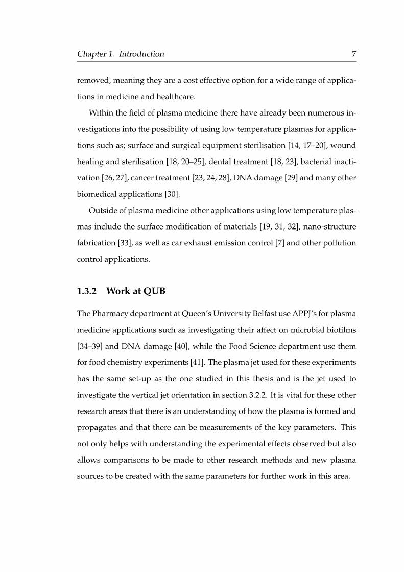
ing to the Townsend mechanism eαd − 1 positive ions are produced in the gap
between the electrodes, distance d in figure 1.2, by each primary electron near
the cathode. αd is known as the amplification paramater.
FIGURE 1.2: Schematic of Townsend breakdown gap [7].
Secondary emission follows and these positive ions return to the cathode and
knock out γ(eαd − 1) electrons, where γ is known as the secondary emission
coefficient. It is defined as the probability of secondary electron emission from
the cathode and is dependent on the type of gas present and the electric field,
as well as the properties of the cathode itself [7]. The discharge is self-sustained
and breakdown occurs when the electric field, and hence α, is sufficiently high
and γ(eαd − 1) = 1. However, if γ(eαd − 1) < 1 the discharge will not be

Chapter 1. Introduction 10
self-sustained [7, 44, 45]. Therefore, the condition for Townsend breakdown to
occur is given by [7]:
γ(eαd − 1) = 1 , αd = ln(1γ+ 1) (1.7)
To obtain an expression for the electric field required for breakdown, Townsend
introduced the similarity parameters α/p and E/p and re-expressed equation
1.6 based on the condition given above and obtained [7]:
α
p= A exp(− B
E/p) (1.8)
where A and B are parameters given in literature for several background gases
at various electric field and pressure values. Combining equations 1.7 and 1.8
results in an expression for the electric field at breakdown as a function of
another similarity parameter, pd, also known as the Paschen curve [7]:
Ep=
BC + ln(pd)
(1.9)
where C = ln A− ln[ln(1/γ + 1)]. The breakdown Paschen curves for various
gases are given in figure 1.3. The minimum voltage at which breakdown can
occur can also be calculated using equation 1.10 :
pdmin =eA
ln(1 +1γ) (1.10)
where e ≈ 2.72 is the base of natural logarithms.

Chapter 1. Introduction 11
FIGURE 1.3: Breakdown Paschen curves for various gases [43].
1.4.2 Streamer mechanism
The theory of the streamer mechanism was initially introduced by Raether [46]
who described a streamer as a thin ionised plasma channel formed due to the
amplification of the electric field by a sufficiently strong primary avalanche.
Secondary avalanches will also be formed due to the photons generated by the
avalanche [43, 46, 47]. When the internal field of an electron avalanche, Ea,
and the external field, E0, are approximately equal, or when the amplification
parameter αd is sufficiently high, the avalanche-to-streamer formation takes
place [7, 43, 44]. This can be given by [7]:
E0 ≈e
4πε0r2a
exp [α(E0
p)x] = Ea (1.11)

Chapter 1. Introduction 12
where ra is the radius of the avalanche head. If ra is assumed to be the same as
the ionisation length, 1/ α, then the streamer formation criterion, also known
as Meek’s breakdown condition, can be given as [7, 43, 47]:
αd (E0
p) = ln
4πε0E0
eα2 ≈ 20 (1.12)
where d is the distance between the electrodes and αd is again the avalanche
amplification parameter. Two types of streamer may form; a positive cathode-
directed streamer or a negative anode-directed streamer.
FIGURE 1.4: Left: Cathode-directed, positive streamer withphotons generated. Right: Anode-directed, negative streamer.Can propagate towards both electrodes. (Adapted from [8]).
A cathode-directed streamer starts near the anode, after the arrival of the elec-
tron avalanche, and propagates in the direction of the cathode due to a high
electric field at the anode. An anode-directed streamer is formed if the elec-
tron avalanche becomes sufficiently strong before reaching the anode and it

Chapter 1. Introduction 13
forms between the electrodes. In this case the streamer propagates towards
both electrodes.
1.4.3 Dawson photo-ionisation theory
However, these descriptions of the formation of the discharge do not explain
the high velocity of the plasma in ambient air, of up to 106 m s−1, consider-
ing the low electric field present. Dawson and Winn [48] attributed this phe-
nomenon to photoionisation in 1965, a theory also proposed by others more
recently investigating plasma jets [42, 49, 50]. Dawson and Winn considered
that the head of the streamer is a sphere of radius r0 and contains n+ positive
ions. Photoelectrons are created at a distance r1 from the centre of the sphere
due to the emission of photons by the streamer. The electrons are accelerated
towards the sphere due to the creation of a high electric field between the pho-
toelectrons and positive ions in the streamer tip and an electron avalanche is
initiated.
FIGURE 1.5: Schematic of streamer propagation (adapted fromLu et. al [50]).

Chapter 1. Introduction 14
In moving from r1 to r2, the electrons form an avalanche of multiplication [50]:
n = exp∫ r1
r2
αdr (1.13)
and diffusion radius:
r0 = (6∫ r1
r2
Dvd
dr)12 (1.14)
where α is again Townsend’s ionisation coefficient, D is the diffusion coeffi-
cient, vd is the drift velocity and r1 is the distance at which attachment and
ionisation rates are equal due to the electric field. In air, this is true when
Ep = 30 V cm−1 mmHg−1 [50]. The electrons will neutralise the positive charge
and a new positive region will be generated if a sufficient number of electrons
are produced by the avalanche. As the streamer propagates a quasi-neutral
ionised channel is left behind [42, 49, 50].
Dawson and Winn [48] outlined three conditions that must be met for streamer
propagation to occur in a low electric field. Firstly, the number of positive ions
newly created by the electron avalanche must be equal to the initial number in
the sphere, n+. Secondly, the diffusion radius of the avalanche head must not
exceed r0. Finally, the electron avalanche must reach sufficient amplification
before the charge regions start to overlap, i.e. 2r0 ≤ r2 [50].
Lu et al. calculated r0 and r2 for several values of n+. Equation 1.13 was
used to calculate r2 when n = n+. Townsend’s first ionisation coefficient, α, in
equation 1.4 is given by:
α = 15p exp(−365pE
) (cm−1) (1.15)

Chapter 1. Introduction 15
where p is the pressure of the gas (ambient air in this case) and E is the electric
field strength. Equation 1.14 was then used to calculate r2 where the diffusion
coefficient, D, is given by:
D =2× 10⁵
p(cm2s−1) (1.16)
where the pressure, p, is in units of Torrs. Table 1.1 shows the resulting values
of r0 and r2 for helium gas [50].
TABLE 1.1: Calculations of r0 and r2 for several values of n+ [50].
Number of original n+ (×109) 1 2 3 4 5
r0 (cm) 0.056 0.068 0.075 0.080 0.085
r2 (cm) 0.02 0.10 0.17 0.23 0.30
It is evident that 2r0 ≤ r2 is only achieved when the number of n+ is greater
than 3× 10⁹ and therefore the streamer propagation can occur in ambient air
under these conditions without an external electric field. This therefore ex-
plains the propagation of plasma in ambient air at velocities of up to 106 m s−1
which agrees with the observations of many others [49–53]. This streamer
propagation into ambient air is essential for the applications described in sec-
tion 1.3.1.
1.4.4 Ionisation wave propagation theory
The possibility that the plasma bullets are produced by the ionisation wave
front has also been considered as this would explain the reproducibility and
stability of the plasma jet [54–57]. Otherwise, both theories have the same
breakdown mechanism, with the crucial processes in the propagation being

Chapter 1. Introduction 16
impact ionisation and photoionisation [54]. However, in this instance, Shi et
al. attribute the high velocity of the plasma to three mechanisms; electron dif-
fusion, the ponderomotive force and the breakdown wave [55].
1.5 Thomson scattering
Thomson scattering is the elastic scattering of free electrons. It is an impor-
tant diagnostic technique that can be utilised to directly measure the electron
density, ne, and electron temperature, Te, of a plasma. Thomson scattering was
first observed when radar pulses were scattered in the earth’s ionosphere, 50
years after J. J. Thomson developed the theory for scattering of electromag-
netic radiation by electrons in 1907 [58]. After the development of lasers in
the 1960’s, Thomson scattering was investigated in laboratories and became
a diagnostic often used in high temperature plasmas. With the introduction
of high repetition rate Nd:YAG lasers came the introduction of Thomson scat-
tering on non-thermal plasmas [59, 60]. More detail on the use of Thomson
scattering will be given in section 2.4 and throughout chapter 5.
1.5.1 Laser-plasma interaction
When a laser is incident on a plasma, the electrons will oscillate with the field
of the laser beam. As they oscillate, the accelerated electrons emit dipole radi-
ation which is detected as the scattered spectrum around the same wavelength
as the incident laser. The Thomson scattering signal is doubly Doppler broad-
ened due to the fast movement of the electrons with respect to the detector
and the incident laser beam [58, 61]. If the oscillations of the electrons are not
Chapter 1. Introduction 17
influenced by neighbouring electrons, this is known as incoherent Thomson
scattering and means the electron density is low [62]. Coherent Thomson scat-
tering is only evident at electron densities greater than 3× 1015 cm−3 [61]. For
the atmospheric plasma discussed in this work, their low electron densities
mean that incoherent Thomson scattering will be present.
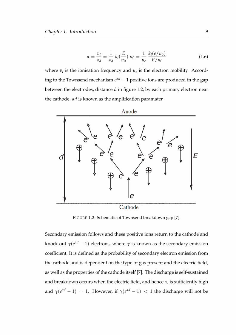
The differential wave vector, k, is defined as the difference between the
wave vectors of the incident laser, k0, and the scattered light, ks. i.e. k = ks− k0
as shown in figure 1.6.
FIGURE 1.6: Vector diagram showing the differential wavevector, k, the incident laser wave vector, k0, and the scatteredlight wave vector, ks. (Adapted from [58]).
In the non-relativistic case, k can be given by:
k =4π
λisin
θ
2(1.17)
where λi is the wavelength of the incident laser and θ is the detection angle
between k0 and ks. The wave vector, k, and the Debye length, λD, are the two

Chapter 1. Introduction 18
parameters which Thomson scattering is dependent on. These two parameters
were combined by Salpeter by introducing the scattering parameter α [62]:
α =1
kλD=
14π sin(θ/2)
λi
λD=
λi
sin(θ/2)(
ne e2
4πkBTe)
12 (1.18)
The magnitude of α is dependent on ne and Te, as well as the incident laser
wavelength, λi, and the scattering angle, θ. If α > 1 this indicates that the
incident wavelength is greater than the Debye length, λi > λD. In this case,
coherent scattering occurs where the incident photons interact with the shield-
ing charges and they undergo group motion. On the other hand if λi < λD
(α < 0.1), then incoherent scattering occurs [58].
The power of the scattered radiation, Pλ, in a solid angle, ∆Ω, at wave-
length λ, is given by [61]:
Pλ(∆Ω) = PinLdσ
dΩ∆Ω φλ(λ) (1.19)
where Pi is the incident laser power, n is the density of the scattering particle, L
is the length over which the interaction takes place, dσdΩ is the differential cross
section, ∆Ω is the solid angle of detection, and φλ contains information of the
spectrum if it is assumed that its integral is equal to 1 [61, 63]. The differential
cross section for Thomson scattering is given by:
dσTS
dΩ= r2
e (1− sin2 θ cos2 ψ) (1.20)
where θ is the scattering angle between the incident and scattered wave vec-
tor, ψ is the angle between the plane of scattering and the polarisation of the
incident laser beam and re is the classical electron radius which is given by [61,
Chapter 1. Introduction 19
63]:
re =e2
4πε0mec2 (1.21)
The differential cross section equation, 1.20, is evidence that Thomson scat-
tering will be maximum in a plane perpendicular to the electric field of the
incident light i.e. when ψ = 90 [64].
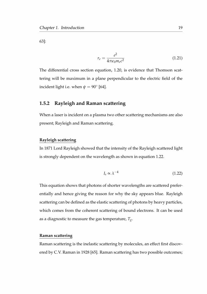
1.5.2 Rayleigh and Raman scattering
When a laser is incident on a plasma two other scattering mechanisms are also
present; Rayleigh and Raman scattering.
Rayleigh scattering
In 1871 Lord Rayleigh showed that the intensity of the Rayleigh scattered light
is strongly dependent on the wavelength as shown in equation 1.22.
Is ∝ λ−4 (1.22)
This equation shows that photons of shorter wavelengths are scattered prefer-
entially and hence giving the reason for why the sky appears blue. Rayleigh
scattering can be defined as the elastic scattering of photons by heavy particles,
which comes from the coherent scattering of bound electrons. It can be used
as a diagnostic to measure the gas temperature, Tg.
Raman scattering
Raman scattering is the inelastic scattering by molecules, an effect first discov-
ered by C.V. Raman in 1928 [65]. Raman scattering has two possible outcomes;

Chapter 1. Introduction 20
a molecule can return to the ground state from an excited state, emitting a pho-
ton of less energy than the incident photon in the process, or a molecule in an
already excited state is excited further and emits a photon of higher energy on
its return to the ground state. These processes are known as Stokes and Anti-
Stokes scattering respectively and are shown in figure 1.7. The wavelength of
a Raman line is specific for each molecule while the intensity of the line in-
dicates the rovibrational distribution [10]. Raman scattering is an important
diagnostic in plasma physics, which provides a means of measuring molecu-
lar densities and the rotational temperature, Trot [66].
FIGURE 1.7: Jablonski diagram for Rayleigh and Ramanscattering, showing the conditions for Stokes and Anti-Stokesscattering to occur.

Chapter 1. Introduction 21
Raman scattering can be up to 3 orders of magnitude greater than the Thomson
signal, while the Rayleigh signal can be up to 5 orders of magnitude greater.
This can lead to experimental difficulties in the detection of Thomson scatter-
ing which will be discussed further in section 2.4.
1.6 Objectives
The main objective of this work was to characterise a low temperature atmo-
spheric pressure plasma jet using a variety of diagnostic techniques to esti-
mate, in particular, electron temperature and electron density of the system.
Initially, we set out to achieve Thomson scattering, however with this proving
a very difficult diagnostic, other techniques were implemented to study the
jet. Imaging on nanosecond timescales was used to not only investigate the
propagation of the plasma plume, but also to estimate the density of excited
states within the plasma using 2D quasi-monochromatic imaging. Emission
spectroscopy was also utilised to discover the species present in the plasma,
both at formation and during propagation, and to estimate the electron tem-
perature. Thomson scattering was also used in an attempt to obtain a more
reliable estimate of the plasma parameters.
1.7 Thesis outline
The rest of this thesis is divided into chapters as follows:
Chapter 2 - Experimental set-up and diagnostics - Details on the set-up for
each experiment and the diagnostics used will be explained in this chapter.
Chapter 3 - Plasma jet imaging - This chapter will describe how imaging on a

Chapter 1. Introduction 22
nanosecond timescale was used to characterise the plasma jet, by not only in-
vestigating the propagation of the plume, but also by using 2D quasi monochro-
matic imaging to estimate the density of helium states present.
Chapter 4 - Emission spectroscopy - This will involve how emission spec-
troscopy was used to estimate the electron temperature, Te, using helium line
ratios and will discuss the assumptions that must be considered, including dis-
cussion on Local Thermodynamic Equilibirum (LTE) and partial LTE (PLTE).
The use of the allowed and forbidden components of helium line emissions to
estimate the electric field will also be investigated.
Chapter 5 - Thomson scattering - This chapter will detail the Thomson scatter-
ing experiment, including the challenges faced. There is also detail of a Raman
scattering model produced to estimate the detection limit for the electron den-
sity, ne, for the system.
Chapter 6 - Conclusions and future work - This chapter will summarise the
results from this work and ideas for future work will also be presented.

23
Chapter 2
Experimental Set-up and
Diagnostics
The aim of this work was to fully characterise an atmospheric pressure plasma
jet (APPJ) using imaging on a nanosecond timescale, optical emission spec-
troscopy and Thomson scattering, as diagnostic techniques. This chapter will
present the experimental set-up required for each of these techniques as well
as some of the early calibration work necessary for the diagnostics. In partic-
ular, Thomson scattering is difficult due to its small cross-section and thus its
low scattering signal. This chapter will detail how the set-up was designed to
overcome these issues as well as being capable of reproducible results.

Chapter 2. Experimental Set-up and Diagnostics 24
2.1 Plasma jet
The plasma jet consisted of a cylindrical quartz tube with inner and outer di-
ameters of 4 mm and 6 mm respectively. Two copper electrodes, each 4.0± 0.5
mm wide, were wrapped around the outer surface of the tube, with the cen-
tre of the powered electrode 6.0± 0.5 mm from the exit of the tube, and the
grounded electrode a further 25.0 ± 0.5 mm away. The powered electrode
was connected to a high voltage pulsed power supply (Haiden PHF-2K) which
had the capability to deliver up to 12 kV peak to peak at a frequency range of
1− 100 kHz. Voltage pulses are used as this reduces the chance of the device
overheating or arcing occuring during long periods of operation [15]. An ap-
plied voltage of around 8 kV was required to initially ignite the plasma. Once
ignited, the voltage could be adjusted to achieve the desired plasma plume. At
higher voltages however, arcing would occur and therefore the voltage always
remained below 8 kV. For experiments described in this thesis, the power sup-
ply was operated at 6− 7 kV and a frequency of 20 kHz.
This plasma jet set-up with two electrodes around a quartz tube, as shown
in figure 2.1, is known as a dielectric barrier discharge (DBD). The applied
voltage was monitored using a Tektronix P6015A voltage probe [67] which was
connected to the powered cable, in close proximity to the powered electrode.
The probe attenuated the voltage by 1000 x which allowed it to be monitored
on an oscilloscope. The current on both the powered and grounded cables was
monitored using Pearson probes [68, 69] as shown in figure 2.1. The current
was also observed on an oscilloscope throughout the experiments. Figure 2.2
shows typical waveforms for the applied voltage and current at both electrodes
during an experiment.
Chapter 2. Experimental Set-up and Diagnostics 25
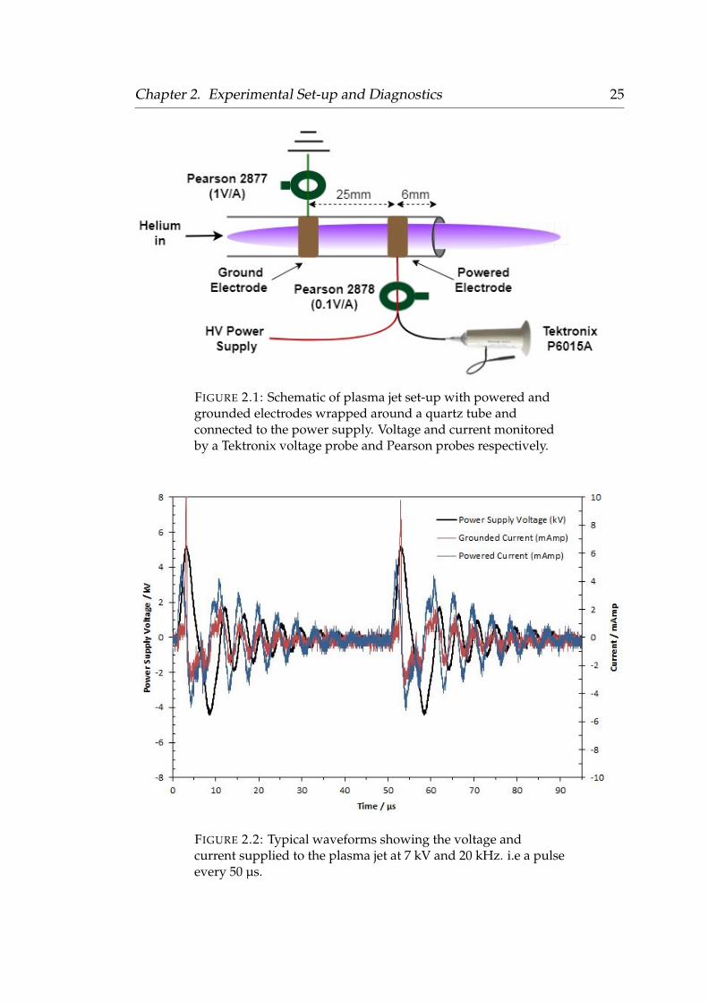
FIGURE 2.1: Schematic of plasma jet set-up with powered andgrounded electrodes wrapped around a quartz tube andconnected to the power supply. Voltage and current monitoredby a Tektronix voltage probe and Pearson probes respectively.
FIGURE 2.2: Typical waveforms showing the voltage andcurrent supplied to the plasma jet at 7 kV and 20 kHz. i.e a pulseevery 50 µs.

Chapter 2. Experimental Set-up and Diagnostics 26
In this case the applied voltage from the power supply was 7 kV at a frequency
of 20 kHz. The voltage reading on the oscilloscope however, was around 5
kV showing the voltage had been attenuated before reaching the oscilloscope.
This may have been due to attenuation in the cables or the t-pieces used to
supply the voltage signal to both the oscilloscope and the delay generators
used in the timing set-up, which will be discussed later. The spikes in the
grounded current which occur just before the peak of the applied voltage, only
appear once the plasma ignites.
2.1.1 Helium gas flow
Helium gas flowing through the quartz tube was necessary, not only to ignite
and sustain the plasma discharge, but also to allow its propagation out of the
quartz tube into ambient air creating a plasma jet. The rate of the helium gas
flow was monitored using either an MKS flow controller or a rotameter. The
rotameter used, however, was calibrated for air and therefore a conversion was
applied to calculate the helium flow rate.
qG = qA
√0.0012
pG(2.1)
Equation 2.1 was used for this conversion where qG is the helium gas flow rate,
qA is the air flow rate reading from the rotameter and pG is the gas density in
gm/ml, which is 1.79× 10⁻⁴ gm/ml for helium. Typically the flow rate was set
to 2 slm on the rotameter, which was equivalent to a 5.2 slm flow rate for he-
lium, with the backing pressure always set to 1 bar. This flow rate is equivalent
to a gas flow velocity of 6.9 ms−1. The Reynolds number is a dimensionless pa-
rameter which can describe whether this gas flow rate will result in a laminar

Chapter 2. Experimental Set-up and Diagnostics 27
or turbulent gas flow. The Reynolds number through a pipe, such as the quartz
tube used in this research can be given by [70],
Re =υ.DH.ρ
µ(2.2)
where υ is the gas velocity, DH is the hydraulic diameter of the pipe, ρ is the gas
density and µ is the dynamic viscosity of the gas. Laminar flow is defined by a
Reynolds number of less than 2100, while turbulent flow is greater than 4000.
At the helium gas flow rates used in this experiment, the Reynolds number
varies from 44 at 1 slm to 234 at 5.2 slm, much lower than 2000, showing that
we expect laminar flow of the gas through the quartz tube.
Helium is easy to ionise due to the efficient production of metastable states
close to the continuum, and is therefore the gas of preference to sustain the
plasma jet. The ionisation energy of helium is 24.6 eV where as the excitation
energies for the metastable states are lower at 19.8 eV for He(23S1) and 20.6 eV
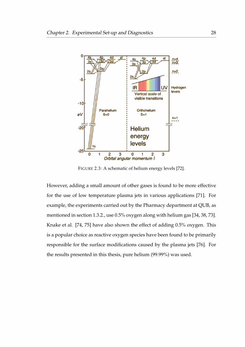
for He(21S1) [71]. As evident in figure 2.3 the triplet state does not return to the
ground state, leading to a build up of helium metastables which accumulate
energy.
Chapter 2. Experimental Set-up and Diagnostics 28
FIGURE 2.3: A schematic of helium energy levels [72].
However, adding a small amount of other gases is found to be more effective
for the use of low temperature plasma jets in various applications [71]. For
example, the experiments carried out by the Pharmacy department at QUB, as
mentioned in section 1.3.2., use 0.5% oxygen along with helium gas [34, 38, 73].
Knake et al. [74, 75] have also shown the effect of adding 0.5% oxygen. This
is a popular choice as reactive oxygen species have been found to be primarily
responsible for the surface modifications caused by the plasma jets [76]. For
the results presented in this thesis, pure helium (99.99%) was used.

Chapter 2. Experimental Set-up and Diagnostics 29
2.2 Imaging
Imaging of the plasma jet required high temporal and spatial resolution which
was provided using a gated intensified charge coupled device (ICCD). The
model used was an Andor iStar (DH334T-18U-63) with 1024 × 1024 pixels,
each 13 µm by 13 µm. It had the capability of a gate width as low as 5 ns and
was always cooled to −30C to minimise the dark current. The photocathode
had a 18 mm diameter aperture with a high peak quantum efficiency(QE) of
47.5% at room temperature, as shown by in figure 2.4.
FIGURE 2.4: Quantum Efficiency data for ICCD camera (Datafrom: [77]).

Chapter 2. Experimental Set-up and Diagnostics 30
The photocathode had a maximum repetition rate of 500 kHz which max-
imised the signal to noise ratio, which is particularly useful in laser based
experiments. There was also a TTL input for external control of the photo-
cathode width and timing using delay generators. The timing set-up required
for each experiment will be detailed in the relevant results chapters.
ICCD gain calibration
The gain settings on the ICCD camera ranged from 0 to a maximum of 4095.
However as this scale was arbitrary, a gain calibration was carried out in order
to establish the gain factor applied to the signal at each of these settings. A
green diode at 532 nm and a red HeNe at 633 nm were used, along with neu-
tral density filters, ND6, to attenuate the signal to ensure the camera was not
saturated. Multiple neutral density filters were used to provide and optical
density (OD) of 6 which corresponds to a transmission of 0.0001 %. The gain
was varied in steps of 500 between the arbitrary values of 0 and 4095, and at
each setting three sets of ten images were recorded with an exposure time of
1 ms. This number of images was to ensure the stability of the beam, while
one image from each set was used in analysis. Figure 2.5 shows a typical green
diode image.

Chapter 2. Experimental Set-up and Diagnostics 31
FIGURE 2.5: Typical green diode image with areas required foraverage background counts numbered 1-4 and the signallabelled as the region of interest (ROI).
In figure 2.5 the four areas numbered 1-4 represent the areas used to calcu-
late the average background counts. This value was then subtracted from the
counts in the region of interest (ROI) to obtain a value for the counts due to
the laser signal. This was carried out for one image from each set of ten. These
were then averaged to find the average counts for that gain setting. At higher
gain settings the exposure time had to be reduced to 0.1 ms to avoid saturation
of the ICCD camera, however this was accounted for in the analysis. This pro-
cess was repeated for each gain setting and using the red HeNe laser. Figure
2.6 shows the resulting gain factor at each gain setting.

Chapter 2. Experimental Set-up and Diagnostics 32
FIGURE 2.6: The effective gain factor applied (log scale) by theICCD to the data at each gain setting, at wavelengths of 532 nmand 633 nm.
Figure 2.6 shows a linear increase in gain factor with the gain setting as well as
the equation used to describe this trend. Similar results for both lasers shows
that the gain factor does not differ over this wavelength range. This gain factor
will become important during analysis in chapter 3.
Chapter 2. Experimental Set-up and Diagnostics 33
2.3 Optical emission spectroscopy (OES)
Emission spectroscopy is a non-intrusive, and relatively simple, diagnostic
technique which can have good spatial and temporal resolution and is able
to give insight into the species present in the plasma as well as methods to es-
timate plasma parameters such as the electron temperature, electron density,
electric field and gas temperature. However, OES is less accurate than Thom-
son scattering for example, as it relies on assumptions such as the plasma being
in Local Thermodynamic Equilibrium (LTE) in order to estimate the electron
temperature using the ratio of spectral line intensities. These calculations and
LTE assumption will be discussed further in section 4.3.
Light is emitted due to transitions from excited states to lower energy lev-
els. These transitions emit a unique spectrum and therefore the species in the
plasma responsible can be determined using OES to identify the spectral lines.
The intensity of each line is an indication of the population of the excited state.
To obtain emission spectra, an Ocean Optics high resolution, broadband
USB spectrometer (HR4000CG-UV-NIR) was used which had a wavelength
range of 200 − 1100 nm and an optical resolution of 0.75 nm FWHM. This
wavelength range covered the emission from helium, the gas used, as well
as nitrogen and oxygen, present in the ambient air as the plasma propagates.
A 1000 µm core diameter bare fiber was clamped 3.0± 0.5 mm above the centre
of the plume and moved along its central axis, collecting spectra both between
the electrodes and along the plasma plume. This distance was verified before
each measurement.

Chapter 2. Experimental Set-up and Diagnostics 34
FIGURE 2.7: Schematic of experimental set-up for emissionspectroscopy.
A bare fiber had the cladding removed at one end so its proximity did not
perturb the plasma, allowing maximum signal detection. However, experience
demonstrated that if the fiber was within 3 mm of the tip of the plume, it would
cause arcing from the plume to the fiber. The fiber had a numerical aperture
(NA) of 0.39, where NA is defined by:
NA = sin α (2.3)
which gives a collection angle, α, for the fiber of 23. Knowing this and the dis-
tance from the fiber to the plasma, 3.0± 0.5 mm, the radius of the detection area
was found to be 1.27± 0.22 mm, resulting in a detection area of 5.1± 1.9 mm2,
and a field of view of 2.5± 0.5 mm along the plasma plume. SpectraSuite, a
program from Ocean Optics, was used to record the data from the spectrom-
eters. Each time three samples were recorded, resulting in the average counts
for each spectral line, accounting for any random fluctuations.
A N2 spectrometer (HR4000) was also used to look at the molecular nitro-
gen emission in the wavelength region 320 − 420 nm. Nitrogen emission in
this region of the spectrum can be used to estimate the gas temperature due

Chapter 2. Experimental Set-up and Diagnostics 35
to the assumption that the molecules of the gas and the molecules in the rota-
tional states are in equilibrium. This is because the rotational excitation only
requires low energies and short transition times [15]. The rotational temper-
ature describes the Boltzmann distribution by which the rotational states are
populated [78], and can be determined by comparing the experimental data to
a simulation using a program written for LabView by Dr. Kari Niemi at QUB,
the results of which can be found in section 4.4.
2.4 Thomson scattering set-up
Thomson scattering is the elastic scattering of free electrons and can be used as
a non-intrusive diagnostic method to investigate the electron density, ne, and
electron temperature, Te. These measurements are essential to form a complete
characterisation of the plasma jet. Previously, it was an approach used in much
higher density discharges and fusion plasmas [79, 80], but is now also used in
low density discharges with temperatures of a few eV. Langmuir probes have
been utilised in the past to estimate these parameters from electron velocity
profiles, however this method can perturb the plasma considerably, generating
unreliable results, as the probe must be in the discharge [58, 81]. Other meth-
ods have included the use of resonator probes and microwave interferometry,
however these techniques cannot provide the temporal or spatial resolution
that Thomson scattering is capable of [63]. It should be noted however, that
at high probing intensities heating of the electrons by inverse bremsstrahlung
may occur, therefore heating the plasma.
Thomson scattering also provides unambiguous results allowing them to
be interpreted easily [82], without the necessity for assumptions regarding the
thermodynamic conditions of the plasma, or the need for techniques such as

Chapter 2. Experimental Set-up and Diagnostics 36
Abel inversion to obtain the measurements. When a laser is used to probe the
plasma jet to investigate Thomson scattering, two other scattering mechanisms
are also present; Rayleigh and Raman scattering, as discussed in section 1.5.2.
Experimental difficulties
Thomson scattering is a difficult diagnostic technique due to the low intensity
of the signal compared to the Rayleigh and Raman scattering, as well as its
high sensitivity to stray light. As previously stated, the Raman signal can be up
to 3 orders of magnitude greater than the Thomson signal, while the Rayleigh
signal can be up to 5 orders of magnitude greater. Rayleigh scattering occurs
at the laser wavelength, 532 nm, and hence there is a spectral overlap with
the Thomson scattering. However, the spectral width of the Rayleigh signal
is much smaller than the width of the Thomson signal and can therefore be
blocked. The Raman, however, cannot be removed as it has a larger spectral
width than the Thomson signal. Therefore, a complex experimental set-up
was required, not only to detect the low signal levels of Thomson scattering,
but also to remove any stray laser light or background signals which may have
affected the response of the system.
2.4.1 Probe laser
The laser used to probe the plasma jet was a Spectra Physics GCR-4 Nd:YAG
laser with q-switching capability. It operated at 10 Hz and was frequency dou-
bled to emit at 532 nm, producing a gaussian laser profile and up to 200 mJ
on target. The beam had a circular shape with a diameter of 9.0± 0.5 mm and
a pulse length of 8 ns full width half maximum, measured using a photodi-
ode. The laser was water cooled to prevent overheating and nitrogen flowed

Chapter 2. Experimental Set-up and Diagnostics 37
through the optical cavity throughout its operation. In order to generate laser
pulses with maximum energy, the time delay between the flash lamps and
pockel cells was set to 220 µs. Figure 2.8 shows a burn of the laser spot just
after it has exited the laser, with a diameter of 9.0± 0.5 mm.
FIGURE 2.8: Burn of laser spot.
2.4.2 Double grating spectrometer
To have any chance of observing Thomson scattering a high resolution double
grating spectrometer was required. The model used was a SPEX 750 which
contained 2 × 1200 l/mm gratings and a series of mirrors to guide the scat-
tered photons to the ICCD which was fitted to the spectrometer. The system
provided a dispersion of 5.7 Å/mm at the detector plane. The entrance slit
could be opened and closed using a micrometer gauge and was generally set
to 0.18± 0.01 mm, a measurement which was verified using feeler gauges.

Chapter 2. Experimental Set-up and Diagnostics 38
FIGURE 2.9: Schematic of double grating spectrometer (Model -SPEX 750). Rayleigh block shown, positioned at the image plane.
A Rayleigh block, a 600 ± 10 µm wire, positioned at the image plane of the
spectrometer, removed the central wavelength of the scattered light to ensure
the Rayleigh scattering at the laser wavelength, 532 nm, did not swamp out
the Raman or Thomson scattering signals.
2.4.3 Plasma jet and laser alignment
As Thomson scattering is an extremely difficult diagnostic technique, a com-
plex experimental set-up was required. Precise alignment and synchronisation
of the system was essential to attempt Thomson scattering and in order to ob-
tain reproducible data.
Initial Plasma Jet Set-up
The plasma jet set-up was contained entirely within an open, cylindrical, stain-
less steel chamber which was remnants from a previous experiment investi-
gating laser ablation, which had required a vacuum [64, 83, 84]. The chamber

Chapter 2. Experimental Set-up and Diagnostics 39
remained part of the set-up in order to reduce the amount of stray light en-
tering the system as well as to act as a safety barrier while the plasma jet was
running. This was the main factor behind mounting the plasma jet horizon-
tally, to allow diagnostics to be positioned around and above the set-up. The
target chamber centre (TCC) was defined using a copper wire mounted on a
magnetic base on a breadboard, and was the point the laser was focused to.
This breadboard could be placed on three bases within the chamber and three
identically positioned bases on an alignment rig. The rig was set up with three
CCDs, one with a top view of the plasma jet, and the other two looking along
the laser axis and jet axis as shown in figure 2.10. With TCC defined on the
alignment rig, it could then be used to position the plasma jet.
FIGURE 2.10: Alignment rig with copper alignment wire andthree CCD cameras, one to define each axis.

Chapter 2. Experimental Set-up and Diagnostics 40
The plasma jet was mounted on a x-y stage, which itself was mounted on
a translation stage which was connected to a motion controller (Newport -
ESP301). This allowed the accurate positioning of the jet within the chamber.
This stage was then mounted on an identical breadboard to that of the align-
ment wire in order to position the plasma jet using the rig. Initially, the plasma
jet was roughly positioned to TCC in the chamber using the translation stage
leaving a lot of movement backwards away from the laser axis, so the laser
would be able to probe along the entire length of the jet. The breadboard was
then placed on the alignment rig and the jet was moved to the TCC position,
earlier defined by the wire, so that the laser axis met the edge of the end of the
quartz tube.
Laser alignment
The GCR laser described in section 2.4.1 was used to probe the plasma jet in
order to look for Thomson scattering. A green laser diode (532 nm) was used
as a reference beam as it was a significantly safer and easier method of aligning
the GCR beam. The full alignment set-up can be seen in figure 2.11. The green
diode beam had three 2-inch silver mirrors directing it into the same beam
path as the GCR beam, the third of which was mounted on a magnetic base
allowing it to be removed when the GCR was in use. These were followed by
three green 2-inch mirrors which directed the beams into the chamber. Green
mirrors were used as they have a high reflectivity and a high damage thresh-
old which is important to remove the IR from the GCR beam. A 1" lens with
focal length of 1 m was then used to focus the beam to a focal spot size of
67.2 ± 5.0 µm FWHM at TCC. Leakage through the second green mirror al-
lowed the energy of the laser pulse to be monitored using a photodiode, while

Chapter 2. Experimental Set-up and Diagnostics 41
leakage through the third green mirror allowed a fraction of the pulse to reach
a CCD camera connected to an alignment monitor, which monitored the posi-
tion of the beam. The green diode beam was aligned to scatter from the top of
the copper wire at TCC and its position was marked on the alignment moni-
tor. The GCR beam was then aligned to overlap the green diode beam on the
alignment monitor, showing that it would also be aligned to TCC in the cham-
ber. To ensure the IR of the GCR beam was filtered out during alignment, a
KG3 filter was used to block it. As an added check, a Mako-CCD camera was
set-up at TCC looking along the laser axis and ensure that both beams over-
lapped at TCC. Before each data set, the alignment could be quickly checked
and adjusted using the marks on the alignment monitor.
Imaging line
A series of mirrors and lenses collected the scattered light and directed it to the
double grating spectrometer. A 300 mm lens above the chamber and another
before the entrance of the spectrometer gave a 1:1 imaging system. A theodo-
lite was set up at the position of the final lens, adjusting the optics accordingly
until a image of the plasma jet was obtained. The final lens was then adjusted
to focus the image onto the entrance slit of the double grating spectrometer.
To ensure the light entering the spectrometer was normal to the slit and was
reaching the ICCD, a green diode was set up in the imaging line. The lid of the
spectrometer was removed to check the beam was hitting the centre of each
mirror, both gratings and the chip of the ICCD.

Chapter 2. Experimental Set-up and Diagnostics 42
FIG
UR
E2.
11:S
chem
atic
ofex
peri
men
tals
et-u
pfo
rTh
omso
nsc
atte
ring
incl
udin
gla
ser
alig
nmen
t,lig
htco
llect
ion
and
imag
ing.
Chapter 2. Experimental Set-up and Diagnostics 43
Stray light reduction
As previously stated, some of the major difficulties when attempting Thom-
son scattering are the low intensity of the signal as well as its small cross sec-
tion. Therefore, it was important that stray light in the system was kept to
a minimum, as it could have a significant effect on the results, especially in
low temperature plasmas with low electron density. Firstly, apertures slightly
larger than the beam diameter were added at the entrance to the chamber. The
laser alignment set-up was also covered during experiments to avoid stray
light from the lab entering the system. To minimise reflections from within
the chamber, the walls, base and any metallic apparatus were lined with an
opaque black material. The same material was used to line the perspex lid
of the chamber, leaving a circular aperture at the centre to allow the scattered
laser light from the plasma jet to be collected at 90. The laser light which
passed through the jet exited the chamber at the opposite side, which had a
beam dump at the end to stop any light being scattered back into the chamber.
The optical table, upon which the imaging line to the spectrometer was situ-
ated, was also covered in an opaque black material and surrounded by blocks
and black cloth to reduce the amount of stray light entering the system. The
imaging optics were also kept clean to reduce the likelihood of light scatter-
ing from dust particles. These steps were important to increase the chance of
observing Thomson scattering.

44
Chapter 3
Plasma Jet Imaging
Imaging on a nanosecond timescale using an intensified charge coupled device
(ICCD) was utilised to characterise the plasma jet. The most effective operat-
ing conditions of the jet were established and the propagation velocity of the
plasma was measured. Changes in the plasma jet’s characteristics depend-
ing on orientation were also studied. 2D quasi-monochromatic images of the
plasma jet were obtained using bandpass filters to isolate the light produced
at individual spectral transitions which allowed the density of excited states
within the plasma to be estimated. Understanding of the key parameters of
the plasma jet is essential for its effective use in applications such as those dis-
cussed in chapter 1.

Chapter 3. Plasma Jet Imaging 45
3.1 Plasma imaging
In order to characterise the plasma and to understand the dynamics of the
plume, the plasma jet was imaged using an ICCD camera to investigate its
temporally resolved emission. Figure 3.1 shows a photo of the plasma jet in
the same configuration as described in section 2.1, with an applied voltage of
7 kV, a frequency of 20 kHz and a helium flow rate of 5.2 slm. The helium gas
flowing through the quartz tube enables the propagation of the plasma into
the surrounding air by creating a helium gas channel. The brightest region of
the jet in the visible region of the spectrum is between the electrodes, while the
plume outside the quartz tube rises at the end due to the buoyancy of helium
in air.
FIGURE 3.1: Photo of plasma jet operating at 7 kV, 20 kHz andwith a helium flow rate of 5.2 slm.
Although the plasma is driven by the applied voltage [16, 49, 85], the helium
gas is required to ignite the plasma and to force the plume out of the quartz
tube, allowing the plume to be probed. The length of the plasma plume out-
side the quartz tube was dependent on both applied voltage and the helium
gas flow rate [16, 30, 49, 54]. It was therefore necessary to ascertain which com-
bination of applied voltage and helium flow rate would provide a long enough

Chapter 3. Plasma Jet Imaging 46
plume to probe while also obtaining a laminar flow without turbulence. This
was found to be using applied voltages of 6− 7 kV and a gas flow rate of 5.2
slm. How this conclusion was reached will be discussed in section 3.2.
The powered and grounded electrodes were switched around, so that the
grounded electrode was closest to the exit of the quartz tube, to investigate
how this would affect the plasma jet. Figure 3.2 shows the resulting plasma jet
operating at the same settings as the jet in figure 3.1.
FIGURE 3.2: Photo of plasma jet operating with the oppositeelectrode configuration, at 7 kV, 20 kHz and with a helium flowrate of 5.2 slm.
This configuration causes the plasma jet to form in the opposite direction,
against the helium gas flow, leaving a very short plume, ∼ 0.5 cm, exiting the
tube into ambient air. This not only rules out this configuration for Thomson
scattering experiments, but also indicates that the plasma is driven by the ap-
plied voltage rather than the gas flow. This is in agreement with observations
by many others [16, 53, 54, 61].
As evident in figure 3.1, the plasma jet appears to be a continuous plume
to the naked eye, however, in 2005 Teschke et al. [53] discovered that the jet
consists of plasma "bullets". Since then many have observed these bullets trav-
elling at velocities on the order of 104 − 105 m s−1 [30, 49–53, 55, 86], much

Chapter 3. Plasma Jet Imaging 47
faster than the helium flow rate, which is more evidence that the plasma bul-
lets are driven by the applied voltage rather than the gas flow [51, 55]. These
plasma bullets were studied to establish their physical and chemical character-
istics such as velocity, size and the species present.
3.1.1 Experimental set-up
The plasma jet was set-up as described in section 2.1. A mirror above the
plasma jet directed the image of the plasma towards the ICCD camera which
was mounted on a breadboard above the chamber containing the set-up. Two
lenses, a 100 mm asphere and a 750 mm achromat lens, were placed on trans-
lation stages to allow the image to be focused easily. These lenses were chosen
to achieve a diffraction limited performance while providing a large collection
efficiency. A filter holder attached to the front of the ICCD was used to mount
bandpass filters for 2D imaging which will be discussed in section 3.3.
FIGURE 3.3: Schematic of experimental set-up for plasma bulletimaging using the ICCD.

Chapter 3. Plasma Jet Imaging 48
A ruler was placed at the quartz tube position and imaged to ensure the system
was focused. The magnification of the system was found to be a demagnifica-
tion of ×7.5, which was equivalent to 0.098 mm per pixel. Due to the high
velocities of the plasma bullets, the system had to be synchronised to ensure
an image of a single bullet could be captured. In this case one Stanford delay
generator (Model DG645) synchronised with the power supply was sufficient
to trigger the ICCD camera to capture an image of a plasma bullet. Figure 3.4
shows the triggering set-up used to image the plasma bullets.
FIGURE 3.4: Schematic of the triggering system to image plasmabullets consisting of a voltage probe, current probes,oscilloscope, Stanford delay generator and an ICCD camera.
A Tektronix P6015A voltage probe [67] connected to the powered electrode
attenuated the pulse by 1000× and the rising edge of this pulse was used to
trigger the Stanford box. The voltage was also monitored throughout the ex-
periment using the oscilloscope along with the current from both the grounded

Chapter 3. Plasma Jet Imaging 49
and powered electrodes, where Pearson current probes were mounted [68, 69].
Although the ICCD camera was triggered manually, the timing was controlled
using the Stanford box which triggered the MCP of the camera to image a
plasma bullet. Delay A on the Stanford box varied the point in time being ob-
served, delay B controlled the size of the time window, while the repetition
rate was controlled by delay C.
3.2 Plasma bullet imaging results
Initial imaging of the plasma jet with exposure times of a few nanoseconds
confirmed the bullet like structure described in section 3.1. Several combi-
nations of applied voltage and helium gas flow rate were tested to find the
optimum settings for the experiments. A turbulent flow would lead to in-
consistency and issues with reproducibility with the experimental results. A
turbulent jet was obvious to the naked eye at applied voltages below 6 kV
or above 7 kV, while plasma bullets were also being produced inconsistently.
This was also observed by Lu et al.[87] who observed that the plasma jet can
display a random behaviour at lower voltages. However, once the voltage is
increased, the repeatable nature of the jet is observed. Walsh et al. [42], us-
ing a similar plasma jet, described this behaviour in terms of three operating
modes: the chaotic mode after the initial gas breakdown, the bullet mode when
the periodic nature of the jet is observed with increased applied voltage, and
continuous mode with a further increase in applied voltage.
The effect of the helium gas flow rate was also considered in order to es-
tablish the optimum set-up, with the conclusion being that 5.2 slm was the
optimum gas flow rate. How this conclusion was reached will be discussed
further in section 3.2.4.

Chapter 3. Plasma Jet Imaging 50
Therefore, the optimum conditions for a plasma jet with minimum turbu-
lence and operating in bullet mode were found to be 6− 7 kV with a helium
gas flow rate of 5.2 slm. These will be the settings throughout this chapter
unless stated otherwise.
3.2.1 Bullet velocity - horizontal jet orientation
Figures 3.5 and 3.6 show plasma bullet images taken every 200 ns to show the
propagation of the bullets with applied voltages of 6 kV and 7 kV for compar-
ison.
FIGURE 3.5: Plasma bullet images throughout propagation at6kV. The plasma exits the quartz tube on the left and travels leftto right. Each image is the accumulation of 100 bullets.
FIGURE 3.6: Plasma bullet images throughout propagation at7kV. The plasma exits the quartz tube on the left and travels leftto right. Each image is the accumulation of 100 bullets.

Chapter 3. Plasma Jet Imaging 51
The velocity of the plasma bullets throughout their propagation was estimated
by measuring the distance travelled by the bullets in the 200 ns time frame. The
position of the front of each plasma bullet was identified from the images using
ImageJ. Their positions were recorded in pixels and the position of the previ-
ous bullet was subtracted to obtain the distance travelled. This distance was
converted to the real distance using the magnitude of the system, a demagni-
fication of ×7.5, and the pixel size, i.e. where 1 pixel was equivalent to 0.098
mm at the object plane. This distance was divided by the time step, 200 ns, to
estimate the plasma bullet velocity over this period of the propagation. These
measurements were repeated twice to calculate an average bullet velocity for
each time step. Figure 3.7 shows the variance in the plasma bullet velocity as
they propagated away from the quartz tube, for applied voltages of 6 kV and 7
kV. The propagation distance given is equivalent to the distance from the exit
of the quartz tube to the front of the plasma bullet.
In both cases the plasma bullets accelerate away from the quartz tube to a
maximum before decelerating, an observation which is consistent with other
studies [49, 52, 54, 86]. Due to the helium metastable states there will be en-
hanced plasma chemistry at the exit of the quartz tube where the helium meets
the ambient air [54]. The acceleration of the plasma bullets as they exit the
quartz tube can therefore be attributed to the diffusion of N2 into the plume
from the surrounding air which can be ionised by the helium metastable states
[88].
With an applied voltage of 6 kV the plasma bullets reached a maximum
velocity of 20± 4 km s−1 at a distance of 8.3± 0.7 mm from the quartz tube,
before decelerating, while at 7 kV the highest recorded velocity was 54 ± 3
km s−1 at a distance of 17± 0.6 mm. The increase in velocity with the increase

Chapter 3. Plasma Jet Imaging 52
FIGURE 3.7: Plasma bullet velocity as a function of propagationdistance with applied voltages of 6 kV and 7 kV.
in applied voltage also agrees with the theory that the plasma is driven by the
applied voltage rather than the gas flow, which is also evident when the bullet
velocities on the order of 105 m s−1 are compared to the gas flow velocity of
6.9 m s−1, at a flow rate of 5.2 slm. Plasma bullet velocities of this magnitude
are consistent with results observed by others investigating similar plasma jets
[49, 51–53, 55, 86]. These significantly high plasma bullet velocities, without
an externally applied electric field, can be attributed to the photo-ionisation
theory first proposed by Dawson and Winn [48]. This is when an electric field
is created between photoelectrons, created by the emission of photons from
the streamer, and positive ions at the head of the streamer. The electric field
accelerates the electrons initiating an electron avalanche, therefore allowing

Chapter 3. Plasma Jet Imaging 53
the streamer to propagate. This theory is described in more detail in section
1.4.3.
The horizontal error bars account for the uncertainty in the position of the
bullet relative to the quartz tube due to the difficulty in gauging the front of
the bullet in the image, as well as for the maximum observed jitter between the
FIGURE 3.8: Visual representation of the maximum observedplasma bullet jitter between consecutive bullets. Vertical lineindicates the position of the front of bullet 1. Bullets 2 & 3indicate a jitter of 0.62 mm to the left and right respectively.
plasma bullets which was ±0.62 mm. The jitter in the bullet position was esti-
mated by recording the position of the plasma bullet in 20 single bullet images
at the same point in time. A visual representation of the jitter between con-
secutive plasma bullets is shown in figure 3.8. The vertical error bars in figure
3.7 were determined by using the uncertainty in the position of the bullet, as
well as the standard deviation between the three measurements recorded for
each time step, to calculate the maximum and minimum possible velocity of
the bullet at this point in time.

Chapter 3. Plasma Jet Imaging 54
FIGURE 3.9: Distance travelled by plasma bullets as a functionof time with applied voltages of 6 kV and 7 kV.
Figure 3.9 shows the same velocity data as figure 3.7 but represented as dis-
tance travelled as a function of time. Results using applied voltages of both 6
kV and 7 kV show a linear increase in distance travelled as time progresses.
However, at 7 kV the plasma bullet travels 33± 1 mm in 1000 ns compared to
12± 1 mm at 6 kV. The data at 6 kV is over a shorter distance as the plume is
much shorter at 6 kV than at 7 kV as, although the gas flow has some affect, the
applied voltage is the main parameter which influences the plume length [49,
54]. A higher applied voltage creates plasma bullets with more energy which
can therefore propagate further along the jet axis at greater velocities [54]. The
errors shown were calculated in the same way as previously described.

Chapter 3. Plasma Jet Imaging 55
3.2.2 Bullet velocity - vertical jet orientation
(downwards propagation)
The same experiment was executed with the only significant differences in the
set-up being the orientation of the plasma jet, which was mounted vertically
with the plume propagating downwards, and the length of the cables from the
power supply to the plasma jet, which were half the length of those used for
the horizontal jet. Orientation is an important factor for applications of the
plasma jet as the tip of the jet will be the area in contact with surfaces and/or
biological material. This experiment was executed using an applied voltage of
6 kV at 20 kHz and a helium gas flow rate of 5.2 slm. Figure 3.10 shows the
plasma bullet velocity results for plasma jet in a vertical orientation.
FIGURE 3.10: Plasma bullet velocity as a function of propagationdistance with jet propagating downwards, at 6 kV.

Chapter 3. Plasma Jet Imaging 56
It is evident from the results that there is the same trend in the velocity of the
plasma bullets. After the final point on the graph the plasma jet becomes too
unstable to obtain any reliable results as the bullets appear to oscillate back and
forth at this stage, an observation also described by Karakas et al. [52]. This
oscillation is from one bullet to the next i.e. the distance travelled by the bul-
lets at this point in time varies more than previously and consecutive bullets
do not necessarily travel further than the previous bullet. Karakas attributes
this observation to the air molecules quenching excited states so the chemical
reactions in the plasma jet are no longer possible, leading to the dissipation of
the plasma jet.
The maximum velocity with the jet mounted vertically is 172± 12 km s−1
which is significantly higher than the highest velocity obtained with the jet
mounted horizontally, which at the equivalent velocity and gas flow settings,
was 20± 4 km s−1. It is therefore obvious that the plasma jets orientation is
critical if high velocities of plasma bullets are to be obtained for the chosen
application. The length of the cables from the power supply to the plasma
jet may also have an affect in this case as the cables for the vertical jet were
approximately half the length (∼ 1.5 m) of the cables used for the horizontal jet
(∼ 3 m). This was due to the positioning of both plasma jet set-ups with respect
to the power supply and this difference may have affected the applied voltage
driving the plasma jet. The affect of different cable length has not yet been
investigated and is a parameter that will be considered in the future. Figure
3.11 shows the distance / time data for this jet orientation.

Chapter 3. Plasma Jet Imaging 57
FIGURE 3.11: Distance travelled by plasma bullets as a functionof time with jet propagating downwards, at 6 kV.
After 220 ns the plasma bullet has propagated 18± 1 mm which is much fur-
ther in comparison to the horizontal jet, where after 1000 ns the plasma bullet
had only propagated 12± 1 mm. Even with an applied voltage of 7 kV and the
horizontal orientation, after 200 ns the plasma bullet had only travelled 6± 1
mm and it took over 600 ns to propagate 18 mm. Therefore, if a longer plume
is required, i.e. necessary that the plasma bullets propagate further, then the
vertical jet orientation is more effective or a higher voltage is required with the
horizontal set-up. This significant difference in velocity may be due to varia-
tions in the gas dynamics when the jet is propagating vertically, or perhaps the
difference in cable length as previously mentioned. Some have suggested that
air entrainment may have a significant impact on the plasma which may also
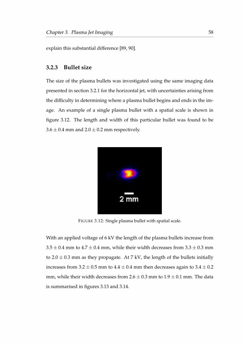
Chapter 3. Plasma Jet Imaging 58
explain this substantial difference [89, 90].
3.2.3 Bullet size
The size of the plasma bullets was investigated using the same imaging data
presented in section 3.2.1 for the horizontal jet, with uncertainties arising from
the difficulty in determining where a plasma bullet begins and ends in the im-
age. An example of a single plasma bullet with a spatial scale is shown in
figure 3.12. The length and width of this particular bullet was found to be
3.6± 0.4 mm and 2.0± 0.2 mm respectively.
FIGURE 3.12: Single plasma bullet with spatial scale.
With an applied voltage of 6 kV the length of the plasma bullets increase from
3.5± 0.4 mm to 4.7± 0.4 mm, while their width decreases from 3.3± 0.3 mm
to 2.0± 0.3 mm as they propagate. At 7 kV, the length of the bullets initially
increases from 3.2± 0.5 mm to 4.4± 0.4 mm then decreases again to 3.4± 0.2
mm, while their width decreases from 2.6± 0.3 mm to 1.9± 0.1 mm. The data
is summarised in figures 3.13 and 3.14.
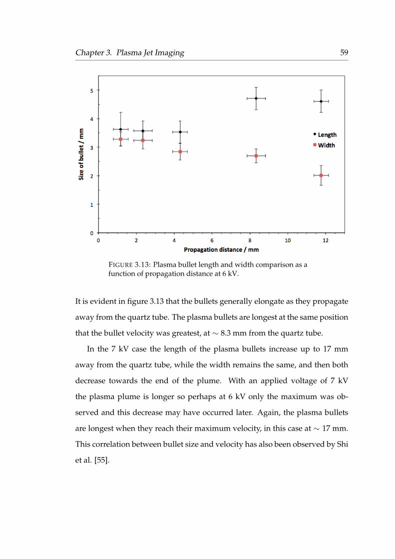
Chapter 3. Plasma Jet Imaging 59
FIGURE 3.13: Plasma bullet length and width comparison as afunction of propagation distance at 6 kV.
It is evident in figure 3.13 that the bullets generally elongate as they propagate
away from the quartz tube. The plasma bullets are longest at the same position
that the bullet velocity was greatest, at ∼ 8.3 mm from the quartz tube.
In the 7 kV case the length of the plasma bullets increase up to 17 mm
away from the quartz tube, while the width remains the same, and then both
decrease towards the end of the plume. With an applied voltage of 7 kV
the plasma plume is longer so perhaps at 6 kV only the maximum was ob-
served and this decrease may have occurred later. Again, the plasma bullets
are longest when they reach their maximum velocity, in this case at ∼ 17 mm.
This correlation between bullet size and velocity has also been observed by Shi
et al. [55].

Chapter 3. Plasma Jet Imaging 60
FIGURE 3.14: Plasma bullet length and width comparison as afunction of propagation distance at 7 kV.
3.2.4 Bullet velocity dependence on gas flow
The studies on bullet velocity and size were carried out using a gas flow rate of
5.2 slm due to the following results when the affect of the gas flow rate on the
plasma bullet velocity and jet length was investigated. These parameters were
studied at four distinct gas flow rates; 1 slm, 2 slm, 3 slm and 4 slm using the
air rotameter, equivalent to 2.6 slm, 5.2 slm, 7.8 slm and 10.4 slm respectively
for helium using the conversion discussed in section 2.1.1. The plasma bullets
were imaged over 200 ns at each gas flow rate and their velocites were calcu-
lated as previously described in section 3.2.1. Figure 3.15 shows the resulting
bullet velocities.
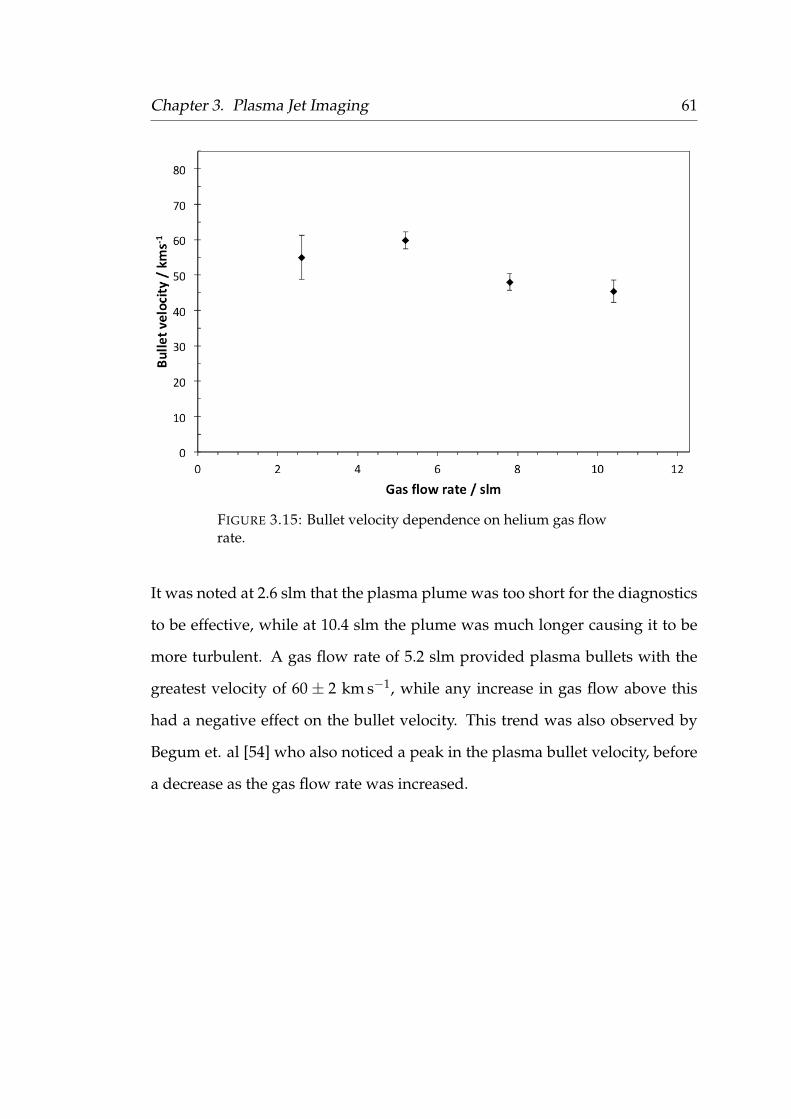
Chapter 3. Plasma Jet Imaging 61
FIGURE 3.15: Bullet velocity dependence on helium gas flowrate.
It was noted at 2.6 slm that the plasma plume was too short for the diagnostics
to be effective, while at 10.4 slm the plume was much longer causing it to be
more turbulent. A gas flow rate of 5.2 slm provided plasma bullets with the
greatest velocity of 60± 2 km s−1, while any increase in gas flow above this
had a negative effect on the bullet velocity. This trend was also observed by
Begum et. al [54] who also noticed a peak in the plasma bullet velocity, before
a decrease as the gas flow rate was increased.

Chapter 3. Plasma Jet Imaging 62
3.3 2D quasi monochromatic imaging
2D imaging was used to estimate the density of excited states within the plasma.
Bandpass filters were used to isolate light produced from different species at
individual spectral transitions to provide 2D quasi monochromatic images of
the plasma jet. The first filter, FB700-10, isolated 706 nm emission from the
excited helium 3S state as it had a central wavelength of 700 nm with a band-
pass of 10 nm. The second filter, FL730-10, was used to isolate emission at 728
nm from the helium 1S state as it had a central wavelength of 730 nm and a
bandpass of 10 nm. These filters were placed in the filter holder in front of the
ICCD as shown in figure 3.3.
Figure 3.16 shows the emission in this region of the spectrum obtained us-
ing a broadband USB spectrometer, as well as the transmission of both filters,
showing that only this helium emission was imaged. With the filter in place
in front of the ICCD to isolate light from a particular transition, images were
recorded of the bullets propagating away from the quartz tube as previously
described. Again the applied voltage was varied between 6 kV and 7 kV while
the frequency was consistently at 20 kHz. The effect of the gain setting on the
ICCD camera was also investigated by varying it from 3500 to the maximum
setting of 4095. However, as discussed previously, these are arbitrary values
and do not represent the absolute gain factor. The gain factors calculated in
section 2.2 will be considered in the analysis.

Chapter 3. Plasma Jet Imaging 63
FIGURE 3.16: Helium emission at 706 nm and 728 nm and thetransmissions of the bandpass filters used. (Transmission datafrom filter manufacturer - Thorlabs).
3.3.1 2D imaging data
Figures 3.17 and 3.18 show examples of the isolated helium emission from 706
nm and 728 nm respectively. Two voltage settings, 6 kV and 7 kV, and two gain
settings on the ICCD camera, 3500 and the maximum of 4095, were studied
for comparison. Images were recorded at intervals of 200 ns for each of these
settings and the images show the propagation of the plasma bullet from right
to left, with each being an accumulation of 10 bullets.
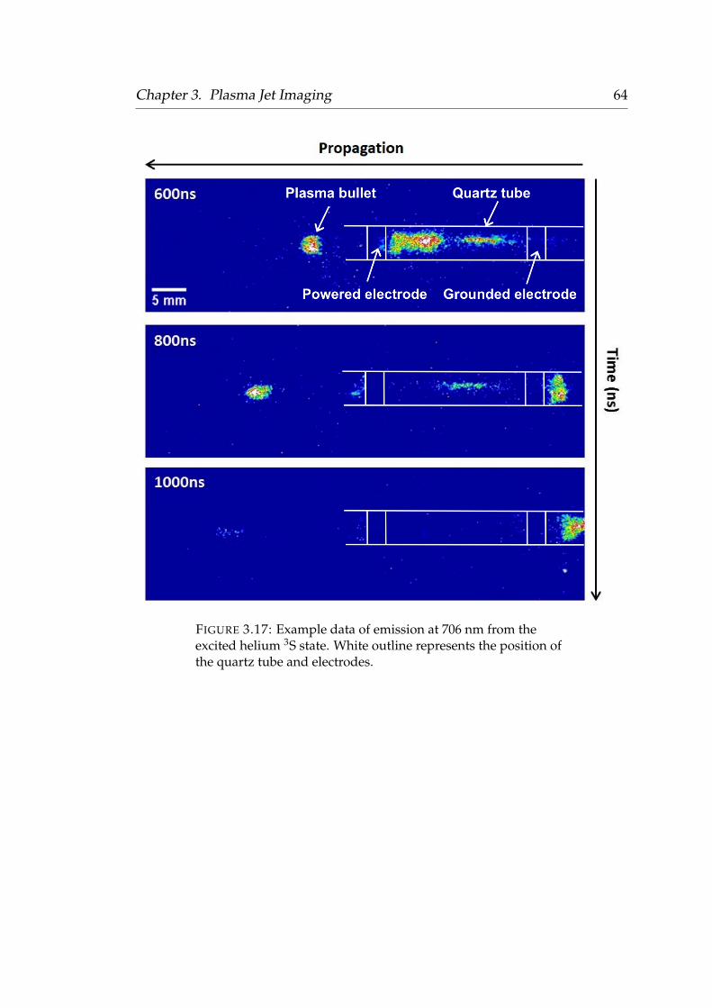
Chapter 3. Plasma Jet Imaging 64
FIGURE 3.17: Example data of emission at 706 nm from theexcited helium 3S state. White outline represents the position ofthe quartz tube and electrodes.
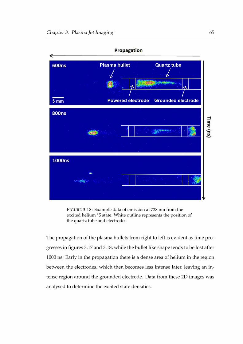
Chapter 3. Plasma Jet Imaging 65
FIGURE 3.18: Example data of emission at 728 nm from theexcited helium 1S state. White outline represents the position ofthe quartz tube and electrodes.
The propagation of the plasma bullets from right to left is evident as time pro-
gresses in figures 3.17 and 3.18, while the bullet like shape tends to be lost after
1000 ns. Early in the propagation there is a dense area of helium in the region
between the electrodes, which then becomes less intense later, leaving an in-
tense region around the grounded electrode. Data from these 2D images was
analysed to determine the excited state densities.

Chapter 3. Plasma Jet Imaging 66
3.3.2 Data analysis method - Abel inversion
As the plasma is observed externally from a side-on view, the intensities ob-
tained are integrated over the full depth of the plasma. A method called Abel
inversion can be utilised to convert the side-on data into a radial distribution
profile by assuming the following [64, 91, 92]:
• the plasma is cylindrically symmetrical,
• the plasma is optically thin, and
• the plasma is stationary during data collection.
It is applied to data from within the tube as this region is most likely to have
cylindrical symmetry. Abel inversion has been implemented on various APPJ
set-ups successfully. The method followed in this case is that of Nestor and
Olsen [93]. The plasma can be split into slices as shown in figure 3.19.
FIGURE 3.19: Slice of an axially-symmetric plasma.

Chapter 3. Plasma Jet Imaging 67
Equation 3.1 is the Abel integral equation, which gives the intensity I(x) [93]:
I(x) = 2∫ R
x
ε(r)r dr
(r2 − x2)12
f or 0 < r < R (3.1)
where x is the distance from the symmetry axis, R is the plasma radius and
ε(r) is the emissivity at a distance r [64, 93]. Abel inversion results in a radial
emissivity of [93]:
ε(r) = − 1π
∫ R
r
I′(x) dx
(x2 − r2)12
(3.2)
However, Nestor and Olsen [93] developed a simpler equation to relate the
emissivity, ε(r), to the intensity, I(x).
fk = −2
πa
N
∑n=k
Bk,n In (3.3)
where
Bk,n = −Ak,k f or n = k (3.4)
Bk,n = Ak,n−1 − Ak,n f or n ≥ k + 1 (3.5)
and
Ak,n =[(n + 1)2 − k2]− [n2 − k2]
12
2n + 1(3.6)
The Bk,n coefficients are tabulated by Nestor and Olsen[93].
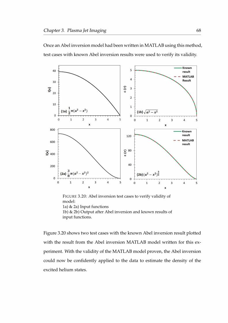
Chapter 3. Plasma Jet Imaging 68
Once an Abel inversion model had been written in MATLAB using this method,
test cases with known Abel inversion results were used to verify its validity.
FIGURE 3.20: Abel inversion test cases to verify validity ofmodel:1a) & 2a) Input functions1b) & 2b) Output after Abel inversion and known results ofinput functions.
Figure 3.20 shows two test cases with the known Abel inversion result plotted
with the result from the Abel inversion MATLAB model written for this ex-
periment. With the validity of the MATLAB model proven, the Abel inversion
could now be confidently applied to the data to estimate the density of the
excited helium states.

Chapter 3. Plasma Jet Imaging 69
3.3.3 2D imaging - Data analysis
The following section will work through an example of the data analysis method
to obtain an estimate of the density of excited helium states. Initially a lineout
was taken vertically through the signal between the electrodes as shown in
yellow in the example in figure 3.21, where the white lines indicate the quartz
tube position and the electrodes.
FIGURE 3.21: Example of lineout through signal for 2D analysis.White lines indicate position of quartz tube and electrodes,while the yellow box indicates the lineout taken.
Any noise or random signal within the data could have an effect on the Abel
inversion and the resulting radial emissivity, ε(r). Therefore, the data was
smoothed before the Abel inversion was applied by taking a 3 pixel average
for each data point. Data smoothing is a technique frequently used before Abel
inversion is applied [64, 92, 94]. The data was plotted and the x-axis was con-
verted from pixel to position in cm using the demagnification of the system,
×7.5.

Chapter 3. Plasma Jet Imaging 70
FIGURE 3.22: Example of lineout data from image in figure 3.21after 3 pixel smoothing.
The following example calculation uses data obtained from the lineout in fig-
ure 3.22 using the 706 nm filter at 6 kV, 1000 ns delay and a camera gain of
3500. The peak counts from the lineout is converted to the number of emis-
sions, Nem, using the following equation:
Nem =4πC
Eγ ICCDres(Gain, λ)QE(λ)T(λ)Ω(3.7)
where C is the peak counts, Eγ is the photon energy, ICCDres is the response
of the ICCD in counts per eV absorbed, while QE is the quantum efficiency
of the ICCD camera and T is the transmission of the imaging system. The
gain, quantum efficiency and transmission of the system are all wavelength
dependent. Ω is the collection efficiency of the imaging system which is only
dependent on the first lens and is given by:
Ω = 2π[1− cos(tan−1(f
2CA))] (3.8)

Chapter 3. Plasma Jet Imaging 71
where f is the focal length of the lens and CA is the clear aperture. For the
system being discussed, f = 750 mm and CA = 45 mm resulting in a collection
efficiency of Ω = 0.0029 sr.
From the lineout in this example and equation 3.7, this gives Nem = 3.22×
105 emissions per sphere. The constants required for this calculation can be
found in table 3.1 for each wavelength.
TABLE 3.1: Constants at each wavelength
706 nm 728 nm
Filter Transmissions (%) 9.89 78.4
QE of ICCD (%) [77] 21.4 10.5
A-rate (s−1) [95] 2.79× 10⁷ 1.83× 10⁷
Degeneracy (g) 3 1
Eγ (eV) 1.76 1.70
ICCDres (Counts/eV) 1290 (max gain) 1430 (max gain)
650 (gain=3500) 720 (gain=3500)
The quantum efficiency of the ICCD camera given in table 3.1 was taken from
the iStar ICCD manual [77] and is also shown in figure 2.4, while the Einstein
A coefficients, or A-rates, were given by NIST [95]. In the case of the 706 nm
emission, there are three spectral lines from the same upper state within a 0.05
nm spread, hence a degeneracy of g = 3. This is due to a splitting of energies as
the transitions from the 3s state drop to the 2p state, which has three possible
values for the total angular momentum. Therefore, the sum of the three A-
rates was used. The 728 nm emission however, is only due to one spectral line
and therefore only one single value for the A-rate is required. The ICCDres
comes from the ICCD calibration previously described in chapter 2.
Chapter 3. Plasma Jet Imaging 72
In order to convert this number of emissions to an excited state density, the
rate at which these excited states will emit photons must be considered. If the
number and rate of emissions from a volume, dv, in a time, dt, is considered,
this gives;
Nem
dvdt= n2A (3.9)
where A is the A-rate, and the total emission time, dt, can be calculated from
the number of plasma bullets imaged, 10 in this case, and the gate width for
each image, 20 ns, resulting in a total emission time of 200 ns. As peak counts
are considered for this calculation, the value being investigated is assumed to
be a column with a 1 pixel by 1 pixel end, and accounting for the magnification
of the system, this results in an area of 9.6× 10⁻⁵ cm2. In order to calculate the
volume, an Abel inversion must be performed to obtain the density profile of
the data.
Due to the assumption that the plasma has a symmetrical profile, the Abel
inversion could be performed on half of the data and mirrored to obtain the
full profile. Therefore, the midpoint of the data had to be established by find-
ing the two points where the intensity was half of the peak counts and iden-
tifying the midpoint between them, a similar method to those used in other
studies [92, 94]. Abel inversion was then performed on the data on one side
of this midpoint with the output after Abel inversion being normalised and
mirrored, obtaining the full profile. The trapezium rule was then used to sum
the normalised data, 6.34× 10⁻² in this case, and using equation 3.10 the peak
density, n2, was calculated.
3.22× 105
dv× (200× 109)= n2 × (2.79× 107) (3.10)

Chapter 3. Plasma Jet Imaging 73
The volume, dv, can now be calculated from the area of the column, 9.6× 10⁻⁵
cm2, and the sum of the normalised data after the Abel inversion, 6.34× 10⁻²,
resulting in a peak density of 9.49 × 109 cm−3 helium 3S states. Figure 3.23
shows the resulting radial profile after Abel inversion as well as the density
of the excited states. The dip in the profile confirms the radial symmetry and
hollow nature of the the plasma plume. This hollow nature has been described
as a ’donut shape’ by many who have observed this by imaging along the jet
axis [49, 53, 87], while also being backed up by computer simulations [96, 97].
Similar to the acceleration of the bullets after exiting the quartz tube, the ’donut
shape’ can be attributed to the diffusion of the surrounding air into the plasma
plume [87, 88]. This was shown by Wu et al. who observed a ’donut shape’
when helium gas was used, but a solid disk shape with a He/N2 mixture,
indicating that it is the diffusion of the nitrogen from the surrounding air into
the plume that creates the ’donut shape’ when only helium is used [88].
FIGURE 3.23: Result of Abel inversion - Density of excitedhelium states

Chapter 3. Plasma Jet Imaging 74
The structure present at ∼ 5.4 cm and ∼ 5.55 cm is real and comes from a peak
in the original data before abel inversion, however more investigation would
be required to discover where this signal comes from. As a check to show
this structure was real, a smooth gaussian profile was also analysed using the
Abel inversion method, which resulted in a profile that did not include these
structures.
It is difficult to quote an exact error for the Abel inversion with ±5− 10 %
quoted in the literature [91, 92, 98]. Data smoothing, although an effective way
to reduce the error in the technique by removing noise in the data, can also be
a source of error if the degree of smoothing is too high [91]. In this instance, the
main source of error comes from determining the midpoint of the data which
will determine the resulting Abel inversion profile. By testing various points
in each data set, the resulting density of helium states was never more than±5
%.
This analysis was repeated to investigate how this density changes through-
out the bullets propagation and with changing voltage. Initially the param-
eters used to scale the results with the gain of the camera were checked by
ensuring the same resulting density was obtained with both gain settings. Fig-
ure 3.24 shows that this was the case, proving the accuracy not only of these
parameters but also the ICCD calibration used to obtain them.

Chapter 3. Plasma Jet Imaging 75
FIGURE 3.24: Comparison of the peak density of helium 3Sstates with different gain settings on the ICCD camera.
Knowing that the parameters used throughout the calculations were accurate,
they could now be used to investigate the effect of voltage on the density of
states and how the density differs for the helium emission at 706 nm and 728
nm.

Chapter 3. Plasma Jet Imaging 76
FIGURE 3.25: Comparison of the peak density of helium 3Sstates at input voltages of 6 kV and 7 kV.
For both 6 kV and 7 kV there is an increase in the peak density for around 400
ns and then a drastic drop in density, similar to the trend seen in the plasma
bullet velocity. The peak is greater at 7 kV as expected with a peak density of
1.98× 1010 cm−3 compared to 9.47× 109 cm−3 at 6 kV.
And finally the resulting density of states for each spectral transition were
compared.

Chapter 3. Plasma Jet Imaging 77
FIGURE 3.26: Comparison of the peak density of helium 3Sstates and helium 1S states over time.
The peak density of the helium 3S emission at 706 nm increases as the bullet
propagates away from the quartz tube to a maximum density of 9.49 × 10⁹
cm−3, and then density decreases again. The peak density of the helium 1S
emission of 12.2× 109 cm−3 at 728 nm, occurs earlier in the plume and then
decreases. This trend is similar to the increase in acceleration of the plasma
bullets during propagation and perhaps shows that peak density occurs when
the velocity of the plasma bullets is at its maximum. Then as the energy of
the plasma bullet dissipates over time, so does the density of states. At 1000
ns the densities are almost equal, around 3× 109 cm−3, for both helium states.
Theoretically, the ratio of the peak densities for the helium states 3S and 1S
can be used to estimate the electron temperature of the plasma. This will be
discussed further in section 4.3.

Chapter 3. Plasma Jet Imaging 78
3.4 Summary
This chapter has focused on using imaging on a nanosecond timescale to inves-
tigate the propagation of the plasma jet as well as the density of states which
produce the plasma. It was found that the jet consisted of plasma bullets trav-
eling with velocities of 20± 3 km s−1 with an applied voltage of 6 kV and with
greater velocities of 54± 3 km s−1 at 7 kV. This increase in velocity with ap-
plied voltage, as well as the fact that these velocities are orders of magnitude
greater than the gas flow rate, showed that the plasma is electrically driven.
The magnitude of the velocities was attributed to a photo-ionisation theory by
Dawson and Winn [48], which was described in section 1.4. These results were
obtained with the plasma jet set up horizontally. However, when mounted
vertically there was a 3x increase in the plasma bullet velocity, perhaps due
to changes in the gas dynamics when the plasma was propagating vertically
downwards. This indicated that the orientation of the plasma jet is crucial for
application purposes.
2D monochromatic imaging was utilised to estimate the density of excited
states. The emission from the helium 3S state at 706 nm and the helium 1S
state at 728 nm was investigated. The method of analysis used to calculate
peak density has been described in detail and focused on the use of an Abel
inversion technique used by Nestor and Olsen [93]. The densities estimated
were in the region of 1 × 109 cm−3 to 2 × 1010 cm−3. The density of states
also followed the same trend as the velocity of the plasma bullets as in both
cases there was an initial increase as the plasma bullets propagated away from
the quartz tube before a decrease. This may suggest that the brightness and
velocity of the bullets may be connected, however this we be discussed further
later once other trends have been established in chapter 4.
79
Chapter 4
Emission Spectroscopy
This chapter discusses how optical emission spectroscopy (OES) was employed
to identify the species present in the plasma jet and how this was used to esti-
mate the electron temperature using helium line ratios and the gas temperature
from nitrogen emission. The electric field was also estimated from the allowed
and forbidden components of the 447 nm and 492 nm helium line emission.
These are key parameters which are required to fully characterise the plasma
jet and are critical in optimising the plasma jet for each specific application.

Chapter 4. Emission Spectroscopy 80
4.1 Experimental set-up
The set-up for emission spectroscopy was as described in section 2.3. Emis-
sion spectra were obtained between 200 − 1100 nm using an Ocean Optics
high resolution, broadband USB spectrometer (HR4000CG-UV-NIR), while a
N2 spectrometer (HR4000) was used to specifically look at nitrogen emission
in the wavelength region 320− 420 nm. For all data discussed in this chapter,
the applied voltage was 6 kV or 7 kV with a frequency of 20 kHz and a helium
gas flow rate of 5.2 slm, unless stated.
This chapter will also discuss emission from the 447 nm and 492 nm helium
lines, which was obtained using the double grating spectrometer described in
section 2.4.3, as shown in figure 4.1.
FIGURE 4.1: Experimental set-up for imaging of heliumemission at 447 nm and 492 nm.
The 1000 µm bare fiber was mounted above the plasma plume. However, this
time the output of the fiber was placed at the plane of the entrance slit of the
double grating spectrometer which was set to a width of 0.20± 0.01 mm, mea-
sured using a feeler gauge. This high resolution spectrometer provided 5.7
Å/mm dispersion at the detector plane. An ICCD camera mounted to the end
of the spectrometer was then used to image the helium emission.

Chapter 4. Emission Spectroscopy 81
4.2 Emission spectra data collection
The most intense spectral lines obtained have been studied to investigate the
species present as well as the behaviour of the plasma as it propagates into
ambient air. Spectral data can give insight into the behaviour of the plasma
bullets as well as estimates for gas temperature, electron temperature, electron
density and the electric field.
4.2.1 Spectra between electrodes
Emission data was collected at 3 positions between the electrodes, 3.2 ± 0.5
mm from the ground electrode, half-way between both electrodes at 12.5± 0.5
mm, and 3.0± 0.5 mm from the powered electrode. All distances were mea-
sured from the centre of the electrodes. Each spectrum was collected during a
3 s exposure and averaged over 3 sets of data. Figure 4.2 shows an example of
data collected half-way between the electrodes. The spectrum is dominated by
helium emission which has a 57 % contribution to the spectrum, which is not
surprising as it is flowing through the quartz tube. Nitrogen and oxygen make
up the rest of the spectrum with 12 % and 32 % contributions respectively. This
is evidence of nitrogen and oxygen gas diffusing into the quartz tube and their
contribution to the spectrum would be expected to rise outside the tube in am-
bient air.

Chapter 4. Emission Spectroscopy 82
FIGURE 4.2: Typical emission spectrum taken between theelectrodes with some of the most intense spectral lines identified.
The spectrum consists of emission from the N2 second positive system (SPS),
(C3Π → B3Π), and from the first negative system (FNS), rotational band N+2
(B2 ∑+u , vB = 0) → N+
2 (X2 ∑+g , vx = 0) around 391 nm. There is also emission
from excited He and O with the most intense helium spectral lines being He
I lines at 587.6 nm (23P − 33D), 667.8 nm (21P − 31D), 706.5 nm (23P − 33S)
and 728.1 nm (21P− 31S), while the oxygen lines are observed at 777.2 nm and
844.6 nm. These observed lines are summarised in table 4.1.
TABLE 4.1: Species identified in plasma (Data from NIST [95]).
Ion N II N I He I He I He I He I He I O I O I
λ/nm 391 427 471 587 667 706 728 777 844

Chapter 4. Emission Spectroscopy 83
Reproducibility of spectra
An important aspect of this experiment was the reproducibility of the plasma
over a period of time. In order to investigate this two spectra were taken, when
the plasma jet first ignited and then 30 minutes later. The fiber was placed
between the electrodes, 9.0± 0.5 mm from the centre of the powered electrode.
In this instance a gas flow rate of 4 slm was used, however this data was only
used to show the reproducibility of the plasma over time and hence the same
gas flow rate as other experiments was not necessary.
FIGURE 4.3: Spectra between electrodes, at the start and end of adata set. Spectra from the end of data set shifted +5 nm.
In the figure above, the spectra taken at the end of the data set has been shifted
by +5 nm in wavelength to allow a direct comparison. It is evident that there
is little change in the species found within the plasma jet over time, with the
largest difference being an ∼ 8 % increase in the intensity of the 391 nm N2

Chapter 4. Emission Spectroscopy 84
line. This could be evidence of nitrogen diffusing into the quartz tube over
time. This consistency in the spectra shows the stability and reproducibility of
the plasma, allowing reliable data to be collected over a long period of time.
4.2.2 Spectra from the plasma plume
Variation with voltage
To understand the affect that voltage has on the species present in the plasma,
two spectra were obtained 8.0± 0.5 mm along the plume of the jet with ap-
plied voltages of 6 kV and 7 kV. Although this is a small variation, significant
differences have been observed in previous experiments (see chapter 3) with
this voltage change.
FIGURE 4.4: Typical emission spectra from plume region of jet at6 kV and 7 kV. Spectra at 7 kV shifted +5 nm.
Chapter 4. Emission Spectroscopy 85
Again one of the spectra, the 7 kV data, has been shifted by +5 nm to allow a
direct comparison. There is a clear increase in the intensity of the spectral lines
with an increase in the applied voltage, as expected and observed by others
[54]. The increase in voltage by 1 kV results in an average intensity increase
of each spectral line of ∼ 30 %. The increase of the 391 nm N+2 line was not
included in this average as the intensity increase in this case was only ∼ 2 %,
significantly lower than the other spectral lines. This could be due to saturation
of the spectrometer at this intensity. In the plume region of the spectrum it is
evident that it is dominated by nitrogen emission rather than helium. Nitrogen
makes a∼ 64 % contribution compared to∼ 23 % and∼ 13 % from helium and
oxygen respectively. This is also a ∼ 53 % increase in nitrogen compared to in-
side the quartz tube, while helium and oxygen have both decreased by ∼ 34 %
and ∼ 19 % respectively. This is not surprising as the helium will dissipate as
the jet propagates in air, while there will be more nitrogen in the air. This large
increase in nitrogen may also be attributed to its diffusion into the plume and
its ionisation by the metastable helium states present, as previously discussed
in chapter 3. If figures 4.3 and 4.4 are compared, it is evident that spectral
lines that appeared in the wavelength range 620− 660 nm between the elec-
trodes, disappear in the spectra obtained from the plasma plume. These lines
can be attributed to the quartz tube which is present when obtaining spectra
between the electrodes, as silicon and oxygen both have spectral lines in this
wavelength range.
Variation in line intensity
The fiber was moved along the plasma jet axis and a spectrum was recorded,
initially 1 mm and 2 mm from the quartz tube, and then every 2 mm along the

Chapter 4. Emission Spectroscopy 86
plume up to 22 mm away. This was executed with an applied voltage of 6 kV
and a gas flow rate of 5.2 slm. Figure 4.5 shows the variation of intensity of
each species in the plasma, nitrogen, helium and oxygen, with the data nor-
malised to the position with the highest intensity, 6 mm away from the quartz
tube. Plasma bullet velocity data from figure 3.7, also with an applied voltage
of 6 kV, is shown in order to compare the trend.
FIGURE 4.5: Line intensity variation of helium, nitrogen andoxygen spectral lines and plasma bullet velocity as a function offiber position, relative to the outlet of the quartz tube.
The initial higher intensity at 1 mm compared to 2 mm could be due to the
initial acceleration of the plasma jet out of the quartz tube which has been at-
tributed to the enhanced plasma chemistry due to helium gas meeting ambient
air as discussed in section 3.2.1. The intensity of each species then increases
along the plume, from 2 − 6 mm, and then decreases along the rest of the
plume as the plasma dissipates. The oxygen intensity decreases most rapidly

Chapter 4. Emission Spectroscopy 87
with the helium and nitrogen decreasing more slowly. This may indicate that
the brightest part of the plasma plume is 6 mm away from the exit of the quartz
tube. This is consistent with the general trend of each individual spectral line.
This increase to a maximum intensity followed by a decrease over the rest of
the plume, a trend also observed by Begum et. al. [54], is consistent with the
trend observed with the plasma bullet velocity. The intensity of each species
reaches its maximum within 2 mm of the peak of the plasma bullet velocity
suggesting a correlation between the bullet velocity and the emission intensity
of the helium, oxygen and nitrogen species.
4.3 Electron temperature estimates using line ratios
Knowledge of the electron temperature and gas temperature is essential to
fully characterise the plasma jet, and critical in order to control them for the
chosen application. For example, for use directly onto human skin, a high elec-
tron temperature is necessary to activate the biochemistry present for the treat-
ment, while a low gas temperature is required to protect the skin and healthy
cells. In order to obtain an estimate of electron temperature, Te, from the emis-
sion spectra, it is generally necessary to assume that the plasma is in local
thermodynamic equilibrium (LTE).
4.3.1 Local thermodynamic equilibrium (LTE)
Thermodynamic equilibrium (TE) is not often found in plasmas in a lab and
may only be found in specific conditions, the interior of stars for example
[99]. In a lab scenario, however, TE may be present in small volumes of the
plasma and in this case it is said to be in Local Thermodynamic Equilibrium

Chapter 4. Emission Spectroscopy 88
(LTE). Griem [100] states that a plasma is in LTE if it is optically thin, homoge-
neous and the free electrons have Maxwellian or Fermi distributions. An LTE
plasma will exhibit similar temperatures of heavy particles and electrons and
will have a high electron density around 1015 − 1020 cm−3 [1, 101], when the
collisional rates exceed the radiative rate by approximately an order of mag-
nitude. This criterion, when the collisional rates are dominant, was expressed
by McWhirter as [99]:
ne 1.6× 10¹² [(T12
e (∆E)]3 (cm−3) (4.1)
where ne is the electron density, Te is the electron temperature and ∆E is the
difference in energy between two states.
If two bound states, n and m, are considered, their electron population ra-
tios can be given by [100]:
Nn
Nm=
gn
gmexp(−En − Em
kTe) (4.2)
where Nn and Nm are the electron populations of the states, gn and gm are
the statistical weight factors or degeneracies, En and Em are the energies of
the states, Te is the electron temperature and k is the Boltzmann constant. This
equation was developed to obtain the Saha equation which considers total den-
sities and defines an LTE plasma [100]:
neni
nm=
2gi
gma30(
kT4πEH
)32 exp(−Emi
kT) (4.3)
where ne is the free electron density, ni is the total ion density and nm is the
total atom density. The degeneracies of the ground state and upper state are

Chapter 4. Emission Spectroscopy 89
given by gi and gm respectively, while EH is the ionisation energy of a hydro-
gen atom, Emi is the ionisation energy and a0 is the Bohr radius. However,
this equation assumes Boltzmann and Fermi statistics and at lower densities
departures from LTE mean the criteria for this equation are no longer met.
Collisional radiative models are required to develop more precise conditions
for LTE [102]. Fujimoto and McWhirter [103] have determined these models
for hydrogen-like ions.
Many plasmas are more likely to exhibit non-LTE or partial LTE character-
istics. A non-LTE plasma will have two temperatures; a heavy particle tem-
perature and an electron temperature, where the electron temperature is much
greater. This is due to fewer elastic collisions as a result of a lower electron
density, < 1013 cm−3, than a LTE plasma, so the heavy particles remain at a
lower temperature [1, 101].
Griem proposed the idea that a plasma is in partial LTE (PLTE) if the col-
lisonal depopulation rate is greater than approximately 10 times the radiative
decay rate [100, 103]. In this case it is possible for the excited states to remain
populated in terms of a Boltzmann distribution and related to the next ion’s
ground state by the Saha equation [102]. The minimum principal quantum
number or collision limit as its also known, ncl, is defined as the lowest level
for which PLTE remains valid to within 10 %. The collisional limit can be esti-
mated using [100]:
ncl ≈ 99n−19
e (4.4)
where ne is in units of cm−3 and ncl is dimensionless.
The excited state populations are determined by the collisional excitation
rates, which can be calculated using the following [104]:
Chapter 4. Emission Spectroscopy 90
< σijv > (m3s−1) = 3.15× 10⁻¹³ f jiRy
Eij(
Ry
T)
12 exp(
−Eij
T) g (4.5)
where f ji is the oscillator strength which is dimensionless and describes the
relative strength of the transition, Ry is the Rydberg energy of the hydrogen
ground state and g is the gaunt factor which in this case is assumed to be the
average, g = 0.2 [104]. The validity of these equations with regards to the
work discussed in this thesis will be tested later.
4.3.2 Electron temperature calculation
The plasma jet used for this work is possibly exhibiting PLTE. However, due
to the complexity of a non-LTE model which would account for all the colli-
sional radiative processes present in the plasma, it is necessary to assume that
the plasma is in LTE. In order to estimate the electron temperature, Te, a line
intensity ratio method is applied which can be used at low densities, as for
helium singlet and triplet states the electron impact excitation rate coefficients
are sensitive to electron temperature, but do not differ with electron density
[105]. The Boltzmann equation below is used to obtain an estimate of electron
temperature using helium line ratios:
Ii
Ij=
Ai
Aj
gi
gjexp
∆Eij
kTe(4.6)
where Ii and Ij are the intensities of two spectral lines with the same ground
states, Ai and Aj are the A-rates of each line, gi and gj are the statistical weight
factors or degeneracies, ∆E is the difference in upper state energies of the two
lines in question, Te is the electron temperature and k is the Boltzmann con-
stant. Ai,j, gi,j and Ei,j were taken from NIST [95] and are shown in table 4.2,

Chapter 4. Emission Spectroscopy 91
and the peak intensity of the spectral lines from the experimental data were
used. As previously stated in section 3.3.3, there are three spectral lines from
the same upper state for the 706 nm line within a 0.05 nm spread and therefore,
the sum of the three A-rates was used. Using equation 4.6 and the information
given in table 4.2, the electron temperature was calculated every 2 mm along
the plasma. The results are shown in figure 4.6.
TABLE 4.2: Spectral lines used in calculation (Data from NIST[95]).
Ion λ/nmA-rate
(×107)/s−1
Upper State
Energy / eVDegeneracy
He I 667.8151 6.37 23.074 1
He I 706.5190 1.55
He I 706.5190 0.93 22.718 3
He I 706.571 0.31
He I 728.1349 1.83 22.920 1

Chapter 4. Emission Spectroscopy 92
FIGURE 4.6: Electron temperature variation along plume using706 nm / 728 nm line ratio. Assuming that the LTEapproximation is applicable.
Figure 4.6 shows the electron temperature results when the 706 nm/728 nm
intensity ratio is used in the described calculation. There is an increase in tem-
perature as the plume propagates away from the quartz tube into the air with
the average temperature across the plume being 0.31 eV. Others have obtained
similar values of electron temperature, for example Hubner et al. achieved
0.1 − 1.6 eV in a 20 kHz DBD jet using Thomson Scattering as a diagnostic
[61]. The fact that the electron temperature is so low suggests that the initial
excitation of the energy levels being considered is by faster electrons being ac-
celerated and this temperature being measured can be thought of as a thermal
background of electrons. Errors in the electron temperature were obtained by
initially assuming a 5% error in the peak intensity observed for each line. The

Chapter 4. Emission Spectroscopy 93
maximum and minimum ratio were then calculated and therefore the maxi-
mum and minimum possible electron temperature were obtained. The error
increases at higher electron temperature as the sensitivity of the equation in-
creases, so a smaller change in the ratio has a large affect on the estimated
temperature. Horizontal error bars arise from consideration of the detection
area.
Several lines with different upper state energies were used in order to test
this approximation. Figure 4.7 shows the resulting temperatures when the 706
nm/667 nm and 728 nm/667 nm intensity ratios were used in the calculation,
in comparison to the 706 nm/728 nm ratio. It is evident in figure 4.7 that when
the other ratios were investigated there was agreement in the electron temper-
ature calculated, showing consistency in the method. This consistency is
FIGURE 4.7: Electron temperature variation along plume,comparison of three line ratios.

Chapter 4. Emission Spectroscopy 94
evident even though the parameters for each ratio are very different, as shown
in table 4.3.
TABLE 4.3: Parameter variation for each line ratio.
706 nm/728 nm 706 nm/667 nm 728 nm/667 nm
∆E /eV 0.20 0.36 0.15
Intensity Ratio 6.2− 14.2 2.4− 12.2 0.34− 0.95
A-rate Ratio 1.52 0.44 0.29
However, the sensitivity of the equation is called into question. Figure 4.8
shows the resulting electron temperature for a range of intensity ratios for each
of the three line ratios. The error bars indicate the difference in the resulting
electron temperature, when the intensity ratio is changed by 1 %.
FIGURE 4.8: Electron temperature (log scale) dependence onintensity ratio for each of the three helium line ratios.

Chapter 4. Emission Spectroscopy 95
For both the 706 nm/728 nm and 706 nm/667 nm line ratios, the electron tem-
perature shows little variance at high intensity ratios. However, the equation is
more sensitive at lower ratios as a small change causes an increasingly larger
change in electron temperature. Also, at lower intensity ratios a 1 % change
causes a significant difference in the electron temperature, whereas at larger
ratios a 1 % change does not have as much of an effect. For example, in the case
of the 706 nm/728 nm ratio, an intensity ratio of 12 will see a 0.96 % change
in electron temperature with a 1 % change in the intensity ratio, where as an
intensity ratio of 4.75 will see a change of up to 34.2 % in electron tempera-
ture. The same trend is observed for both of the other line ratios. However,
there is noticeable variation in the electron temperature around 0.3 eV for each
line ratio, therefore consolidating the result by showing that the agreement be-
tween all three line ratios was not due to the insensitivity of the equation at
high intensity ratios.
4.3.3 Other results using electron temperature
Using the average electron temperature obtained, 0.31 eV, the electron density
can be estimated, again assuming LTE using the Saha equation [100]:
neni
nm=
2gi
gma30(
kT4πEH
)32 exp(−∆E
kT) (4.7)
For this calculation it is assumed that ne ≈ ni, gi = 2 and gm = 3 for the
degeneracy of the upper state, while the peak density of helium 3S states of
9.47× 109 cm−3 from section 3.3.3 is used as nm. This results in an electron
density of ne = 1.1× 1014 cm−3 which is perhaps an upper limit for this sys-
tem.
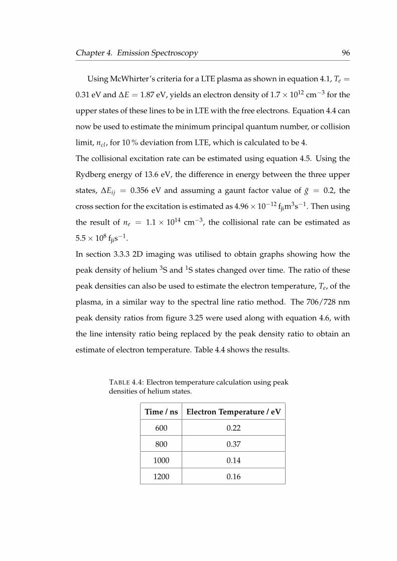
Chapter 4. Emission Spectroscopy 96
Using McWhirter’s criteria for a LTE plasma as shown in equation 4.1, Te =
0.31 eV and ∆E = 1.87 eV, yields an electron density of 1.7× 1012 cm−3 for the
upper states of these lines to be in LTE with the free electrons. Equation 4.4 can
now be used to estimate the minimum principal quantum number, or collision
limit, ncl, for 10 % deviation from LTE, which is calculated to be 4.
The collisional excitation rate can be estimated using equation 4.5. Using the
Rydberg energy of 13.6 eV, the difference in energy between the three upper
states, ∆Eij = 0.356 eV and assuming a gaunt factor value of g = 0.2, the
cross section for the excitation is estimated as 4.96× 10⁻¹² fjim3s−1. Then using
the result of ne = 1.1 × 1014 cm−3, the collisional rate can be estimated as
5.5× 10⁸ fjis−1.
In section 3.3.3 2D imaging was utilised to obtain graphs showing how the
peak density of helium 3S and 1S states changed over time. The ratio of these
peak densities can also be used to estimate the electron temperature, Te, of the
plasma, in a similar way to the spectral line ratio method. The 706/728 nm
peak density ratios from figure 3.25 were used along with equation 4.6, with
the line intensity ratio being replaced by the peak density ratio to obtain an
estimate of electron temperature. Table 4.4 shows the results.
TABLE 4.4: Electron temperature calculation using peakdensities of helium states.
Time / ns Electron Temperature / eV
600 0.22
800 0.37
1000 0.14
1200 0.16

Chapter 4. Emission Spectroscopy 97
These electron temperature results are similar to the average electron temper-
ature calculated to be 0.31 eV. The trend is also interesting as the electron tem-
perature increases to a peak and then decreases again, a similar trend already
found when investigating bullet velocity and the line intensity variation along
the plume. This suggests that as the plasma bullet reaches its peak velocity, the
electron temperature may also be reaching its peak. These values of electron
temperature seem low compared to others in the field [63, 66, 106], however
some, such as Hübner et al., have observed similar values in a 20 kHz DBD jet
[107].
4.4 Nitrogen spectra and gas temperature
As described in chapter 2 nitrogen emission can be used to estimate the gas
temperature due to the molecules in the gas and in the rotational states being
in equilibrium [15]. Therefore, the rotational temperature is a good indicator
of the gas temperature. Using a N2 spectrometer (HR4000) nitrogen emission
in the wavelength range 320− 420 nm was observed. In this instance the ap-
plied voltage was 6 kV at 20 kHz, with a helium flow rate of 5.2 slm. Data was
taken using a 30 second scan and three scans were averaged. The fiber was
placed 12± 0.5 mm, approximately half way, along the plasma plume and the
spectrum obtained is shown in figure 4.9.

Chapter 4. Emission Spectroscopy 98
FIGURE 4.9: Typical emission spectrum from the second positivesystem and first negative system of nitrogen [(0-0), (0-1) etc.denote vibrational numbers].
Figure 4.9 shows a nitrogen spectrum consisting of emission from the second
positive system (SPS), (C3Π → B3Π), and the first negative system (FNS), ro-
tational band N+2 (B2 ∑+
u , vB = 0) → N+2 (X2 ∑+
g , vx = 0) around 391 nm. The
lines and vibrational numbers were identified using a spectrum from Loureiro
et al. [99]. In order to determine the gas temperature the spectra was compared
to simulated spectra using a LabView program written by Dr. Kari Niemi at
Queen’s University Belfast. It was used to fit a curve to the C3Π → B3Π rota-
tional band at 380 nm.
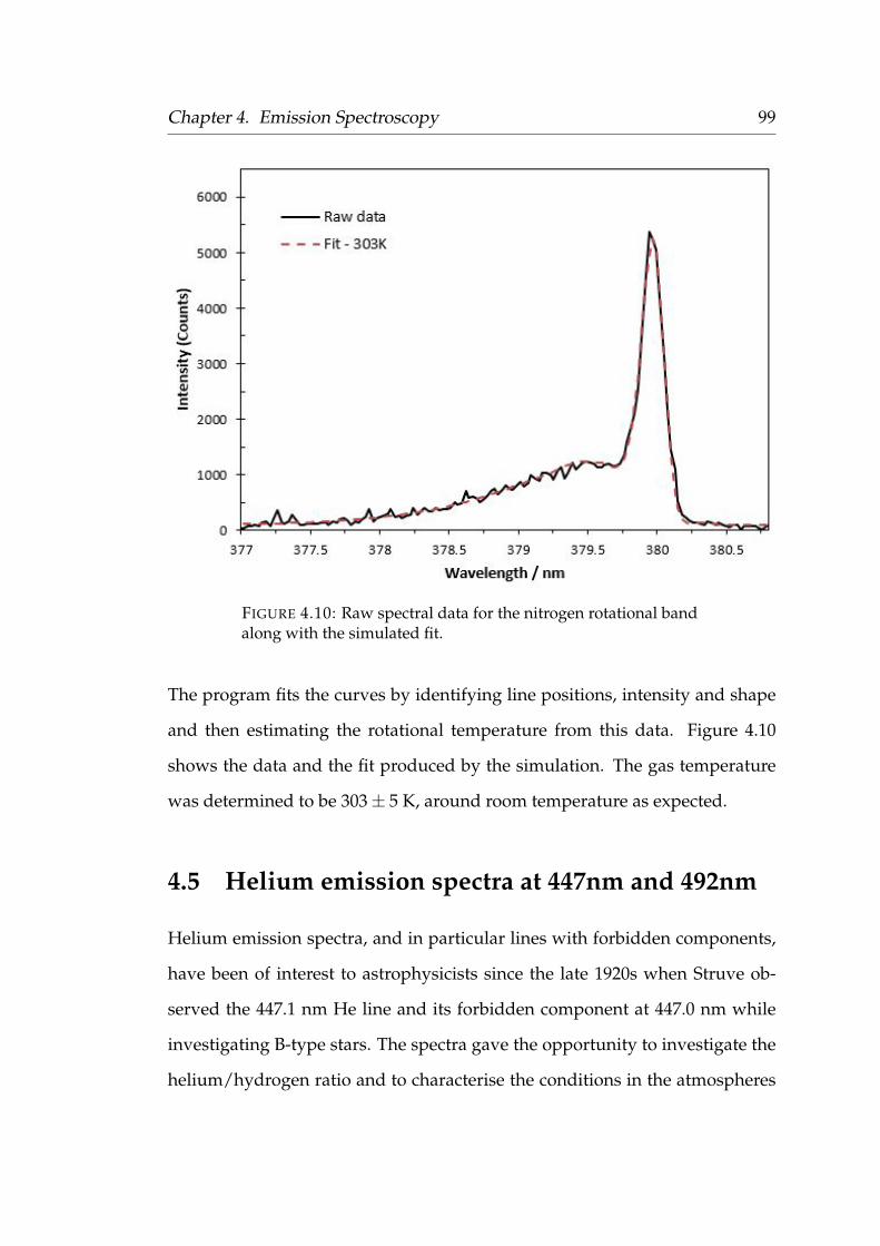
Chapter 4. Emission Spectroscopy 99
FIGURE 4.10: Raw spectral data for the nitrogen rotational bandalong with the simulated fit.
The program fits the curves by identifying line positions, intensity and shape
and then estimating the rotational temperature from this data. Figure 4.10
shows the data and the fit produced by the simulation. The gas temperature
was determined to be 303± 5 K, around room temperature as expected.
4.5 Helium emission spectra at 447nm and 492nm
Helium emission spectra, and in particular lines with forbidden components,
have been of interest to astrophysicists since the late 1920s when Struve ob-
served the 447.1 nm He line and its forbidden component at 447.0 nm while
investigating B-type stars. The spectra gave the opportunity to investigate the
helium/hydrogen ratio and to characterise the conditions in the atmospheres

Chapter 4. Emission Spectroscopy 100
of B-type stars [108], while others have used the 447.1 nm helium line to in-
vestigate Stark broadening theories [109]. The 447.1 nm He line along with the
492.2 nm He line are two of the strongest spectral lines which exhibit forbidden
components which are induced by the plasma microfield [110]. The significant
intensity of these lines and the forbidden components, as well as the notice-
able wavelength shifts and changes in the full-width half-maximum (FWHM)
with electric field and electron density, make these lines suitable to investigate
these parameters. The unshifted allowed and forbidden components of the
447.1 nm He emission line originate from the 43D− 23P and 43F− 23P tran-
sitions at 447.1 nm and 447.0 nm respectively [109]. While for the 492.2 nm
He emission line the allowed and forbidden components originate from the
41D− 21P and 41F− 21P transitions at wavelengths of 492.2 nm and 492.0 nm
respectively [111].
An allowed transition has a high probability of occurring, where as a for-
bidden transition has a much lower probability as it will not occur under typi-
cal conditions. In high density regimes the probability of a radiative transition
is suppressed by collisions before emission occurs [112]. These forbidden lines
will arise in lower density regimes when a transition from a metastable state
occurs.
The electron density, ne, of a plasma source can be determined through
measurements of several parameters of the line profiles of both the allowed
and forbidden lines. These include; the ratio of the peak intensities of the al-
lowed(A) and forbidden(F) components, IF/IA, the ratio of the dip between
the components and the peak intensity of the allowed line, ID/IA, the separa-
tion between the peaks, SAF, and total FWHM of the components, ∆λAF [113].
While many of these parameters are easily measured, SAF is the most reliable

Chapter 4. Emission Spectroscopy 101
as it is independent of any background in the spectra and is solely a function
of the electron density.
FIGURE 4.11: Parameters of allowed and forbidden linesidentified.
However, it has been found that some parameters work better than others de-
pending on the electron density. For example, Perez et al. [114] found the sep-
aration parameter, SAF, and the FWHM to be the most useful methods at their
electron density range of 1.5× 10¹⁶ − 1.45× 1017 cm−3. Where as, Adler and
Piel [110] found that SAF showed little variation with electron density at low
densities while IF/IA exhibited a large variation at lower densities compared
to the other parameters, hence favouring the intensity ratio as a diagnostic
at lower densities. Many have developed formulae to calculate the electron
density from these line parameters. Perez et al. [114] compared experimental

Chapter 4. Emission Spectroscopy 102
results, from a pulsed arc plasma in pure helium, to previous results and the-
oretical data to develop the following expressions relating the density to the
FWHM and separation of the lines for the 447.1 nm line [114]:
log(ne) = log(∆λAF) + 22.357− 0.0209∆λAF , (4.8)
log(ne) = 21.790 + 1.436√
SAF − ∆λ0 (4.9)
where ne is in m−3, ∆λAF and SAF are in nm and ∆λ0 = 0.1557 nm is the sepa-
ration between the unperturbed 447 nm allowed and forbidden lines according
to Moore [115]. Similarly, for the 492.2 nm line [114]:
log(ne) = log(∆λAF) + 22.190 + 0.02506∆λAF , (4.10)
log(ne) = 21.530 + 1.173√
SAF − ∆λ0 (4.11)
where ∆λ0 = 0.1579 nm is again the separation between the unperturbed
492nm lines [115]. Perez quotes these equations as being valid in the density
range 1.5× 10¹⁶ − 1.45× 1017 cm−3, however other parameters may be more
suitable in other density ranges.
Czernichowski and Chapelle [116] used the following formula relating the
separation and electron density for the 447.1 nm line:
log(ne) = 17.056 + 1.586 log(SAF − 0.156) + 0.225[log(SAF − 0.156)]2 (4.12)
where ne is in cm−3 and SAF is in nm. They also used the following equation
Chapter 4. Emission Spectroscopy 103
relating the ratio of the peak intensities of the allowed and forbidden lines,
F/A, and the electron density for the 447.1 nm line:
log(ne) = 16.563 + 1.658 log(FA) + 0.257[log(
FA)]2 (4.13)
Both equations are valid for the density region 2× 10¹⁴ − 2× 1016 cm−3 with
an estimated uncertainty for ne of ±13 % [116].
These helium emission lines can also be used to determine the electric field
in the plasma. Cvetanovic et al. developed an equation relating the separation
and the electric field for the 492.2 nm line [117]:
E(kVcm−1) = (−58.557 + 18.116SAF + 3130.96S2AF + 815.6S3
AF)12 (4.14)
This is valid in the electric field region 1 − 100 kVcm−1 where the 492.2 nm
line and its forbidden counterpart are easily resolved as there is a high enough
field. This method was experimentally verified using a glow discharge and
compared to other methods to ensure its reliability. It is a particularly useful
method as the electric field can be estimated without the need for any other
plasma parameters. Figures 4.12 and 4.13 show the data from Cvetanovic et al.
[117] which was used to, not only estimate the electric field using the 447.1 nm
and 492.2 nm emission line results but also in order to establish equation 4.14
for the electric field for the 492.2 nm line.

Chapter 4. Emission Spectroscopy 104
FIGURE 4.12: Electric field determination using separationbetween the allowed and forbidden components of the 447.1 nmline (where m=0 and m=1 denote transitions [0-0] and [1-1]respectively) [117].

Chapter 4. Emission Spectroscopy 105
FIGURE 4.13: Electric field determination using separationbetween the allowed and forbidden components of the 492.2 nmline (where m=0 and m=1 denote transitions [0-0] and [1-1]respectively) [117].
However, the separation of the lines, SAF, cannot be used to determine
both the electron density and the electric field as one parameter will dom-
inate. The validity of the equations by both Perez and Czernichowski and
Chapelle, which cover density ranges of 1.5 × 10¹⁶ − 1.45 × 1017 cm−3 and
2× 10¹⁴− 2× 1016 cm−3 respectively, are in electron density regimes which are
orders of magnitudes higher than the density of the plasma jet being consid-
ered here. Therefore, the results from this experiment will focus on estimating
the electric field using equation 4.14, which is valid for electric fields between
1− 100 kVcm−1, and figures 4.13 and 4.14, which are valid for electric fields
over 2 kV cm−1 [117].

Chapter 4. Emission Spectroscopy 106
4.5.1 447nm results
The setup for this experiment was as described in section 4.1. A double grat-
ing spectrometer and ICCD camera were used to image the helium emission
from the 447 nm and 492 nm allowed and forbidden components at an applied
voltage of 7 kV. Figure 4.14 shows the resulting spectra for the 447.1 nm line.
The inset is the raw data image, which is 10 accumulated images, each with an
exposure time of 1 s.
FIGURE 4.14: Lineout of 447.1 nm He line with forbiddencomponent. (Inset: ICCD image of data with lineout positionshown).
The allowed and forbidden components are clearly visible in figure 4.14 as well
as a N2 ro-vibrational state. The separation, SAF, of the allowed and forbidden
lines in this case was 0.55 ± 0.03 nm. Using figure 4.12 from Cvetanovic et

Chapter 4. Emission Spectroscopy 107
al.[117], an estimate for electric field can be estimated as 36± 2 kV cm−1. Many
have reported observing a field free (ff) component in the spectra of various
discharges [117, 118], however in this case it does not appear due to it being
below the detection threshold.
4.5.2 492nm results
The same set-up was used to image the 492 nm helium emission. Figure 4.15
shows the allowed and forbidden lines along with an inset of the data image
which is an accumulation of 10 one second exposures. In this case the fiber
was moved along the plasma jet in 1mm intervals, from an initial 3 mm away
up to 9 mm away from the exit of the quartz tube.
FIGURE 4.15: Lineout of 492.2 nm helium line with forbiddencomponent, 7 mm along plume (Inset: ICCD image of data withlineout position shown).

Chapter 4. Emission Spectroscopy 108
The separation between allowed and forbidden components in this case varied
from 0.53− 0.56 nm along the plume. This separation resulted in an average
electric field of 32.1± 1.2 kV cm−1 using equation 4.14. This method is time
resolved as the majority of the light was collected as a bullet passed, or when
the electric field was at its maximum. In order to obtain an estimate from
figure 4.13, the separations between the allowed transition and the forbidden
transition at each point along the plume were calculated and the average used
as the separation, SAF. This method gave an electric field of 32.1± 1.3 kV cm−1,
in agreement with the equation. The results for each position along the plume
are shown in figure 4.16 below.
FIGURE 4.16: Electric field variation along plasma plume.

Chapter 4. Emission Spectroscopy 109
The graph shows an almost constant field around 32 kV cm−1. This is consis-
tent with the findings of Sretenovic et al.[118] who also used emission spec-
troscopy to obtain the separation between the allowed and forbidden compo-
nents of the 492.2 nm helium line, which resulted in an almost constant field
of around 20 kV cm−1.
FIGURE 4.17: Axial electric field in plasma jet by Sretenovic etal.[118]. Consistent with results in figure 4.17.
Their findings of a 20 kV cm−1 electric field with an applied voltage of 4 kV is
consistent with these results, electric fields of 32 kV cm−1 and 36 kV cm−1 for
the 492 nm and 447 nm emission lines respectively at an applied voltage of 7
kV. The experimental results from Sretenovic et al. are also in good agreement
with a 2D model [97, 119], that simulates the propagation of low temperature
helium jets by considering the electric field and the number densities of the
charged species present.
There are few other cases to compare this data to in the literature which
use a similar plasma jet. However, similar methods have been used on various
other plasma jet setups. For example, Kuraica et al. observed electric fields
of up to 18 kV cm−1 in a glow discharge [120], while Obradovic et al. mea-
sured an electric field of up to 11 kV cm−1 in a DBD plasma jet in a helium
environment which only had a 2 mm separation between the electrodes [111].

Chapter 4. Emission Spectroscopy 110
Examples of using the intensity ratio, IF/IA, rather than the separation can
also be found [114, 121].
4.6 Summary
This chapter has taken an extensive look at the results from optical emission
spectroscopy. Initially, the species present in the plasma jet were identified
with the results showing that helium dominated the spectra from between the
electrodes, while nitrogen was more dominant in the plume region outside the
quartz tube. This may be attributed to nitrogen diffusing into the plume which
can then be ionised by the helium metastable states. There was also an increase
in the intensity of the spectral lines with applied voltage as expected, and the
reproducibility of the spectra over time was confirmed.
The trend in line intensity across the plasma plume was consistent with the
trend observed in the plasma bullet velocity in chapter 3. That is, there is an
increase to a maximum intensity, possibly linked to the acceleration of the of
the plasma bullets, followed by a decrease in intensity across the rest of the
plume as the plasma dissipates.
The electron temperature of the plasma was estimated to be 0.31 eV using
helium line ratios and assuming that the plasma is in LTE. This results validity
was confirmed using the results from three different line ratios.
The gas temperature was determined by analysing nitrogen emission and
comparing it to a simulation. The result of which showed a gas temperature of
303 K, around room temperature as expected.
The electron density was also determined using the separation of the al-
lowed and forbidden components of the helium emission at 447 nm and 492
nm. The emission at 447 nm yielded an electric field of 36± 2 kV cm−1, while

Chapter 4. Emission Spectroscopy 111
at 492 nm an electric field of 32.1± 1.2 kV cm−1 was estimated. These results
were consistent with other studies in the field.

112
Chapter 5
Thomson Scattering
Thomson scattering as a diagnostic for the measurement of the electron den-
sity and electron temperature of the plasma jet will be studied in this chapter.
Experimental challenges for this diagnostic include the alignment and stabil-
ity of the system in order to ensure the reproducibility of the results, as well
as the low intensity of the Thomson scattering signal. Thomson scattering has
not been observed in this case, however, it was possible to estimate the upper
limit of the electron density of the plasma by establishing the detection limit
of the system using a Raman model. No evidence of Thomson scattering was
observed above the systems detection limit of electron density of 9.95× 10¹²
cm−3. Hübner et al. observed Thomson scattering using a similar plasma
jet and a triple grating spectrometer, measuring electron densities as low as
5× 1012 cm−3 [107]. A double rather than a triple grating spectrometer was
used in this investigation which may explain why it was not possible to ob-
serve Thomson scattering.

Chapter 5. Thomson Scattering 113
5.1 Initial set-up
Thomson scattering is a powerful diagnostic for plasma characterisation as it
provides a non-intrusive method of determining parameters of a plasma, such
as electron density and electron temperature. It can be used without the need
of assumptions such as the LTE assumption used in chapter 4, and without
the need for techniques such as Abel inversion, as seen in chapter 3. Due to
the low signal levels associated with Thomson scattering, a complex set-up is
required.
The Thomson scattering set-up is as described in section 2.4.4. Before com-
mencing the experiment, the position of the plasma jet was set to the target
chamber center (TCC) using the alignment rig as previously described. The
green alignment laser was directed to TCC and its position marked on the
alignment monitor. The GCR beam was then aligned to the same position on
the alignment monitor, overlapping the two beams ensuring the GCR beam
was hitting the plasma plume. In order to have the greatest possibility of
observing Thomson scattering the brightest part of the plasma jet was to be
probed. A Mako CCD was set-up at the end of the chamber, imaging along the
laser axis, to image the plasma jet and the laser focus position. In order to im-
age the laser it was set to the minimum energy where detection was possible,
while a neutral density filter, ND 5, was also placed in the beam path to pro-
tect the CCD. It was evident that the most intense region of the jet was a few
mm away from the end of the quartz tube and at the lower edge of the plume.
Using the translation stage the jet was moved back by 3 mm, away from TCC,
allowing the laser to probe the brightest region. Figure 5.1 shows the plasma
jet running at the typical conditions of 7 kV, 20 kHz and 5.2 slm helium flow
rate, along with the focal spot of the laser in the plume which has a diameter
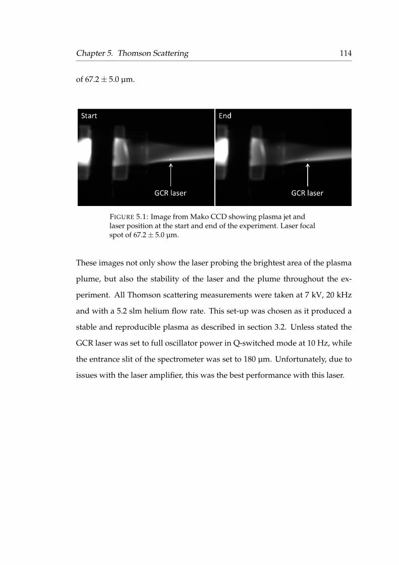
Chapter 5. Thomson Scattering 114
of 67.2± 5.0 µm.
FIGURE 5.1: Image from Mako CCD showing plasma jet andlaser position at the start and end of the experiment. Laser focalspot of 67.2± 5.0 µm.
These images not only show the laser probing the brightest area of the plasma
plume, but also the stability of the laser and the plume throughout the ex-
periment. All Thomson scattering measurements were taken at 7 kV, 20 kHz
and with a 5.2 slm helium flow rate. This set-up was chosen as it produced a
stable and reproducible plasma as described in section 3.2. Unless stated the
GCR laser was set to full oscillator power in Q-switched mode at 10 Hz, while
the entrance slit of the spectrometer was set to 180 µm. Unfortunately, due to
issues with the laser amplifier, this was the best performance with this laser.

Chapter 5. Thomson Scattering 115
5.2 Synchronisation
5.2.1 Triggering system
Synchronisation of the plasma jet, ICCD camera and GCR laser was essential
in order to, not only image the laser scattering from the plasma, but to ensure
the laser pulse was striking a plasma bullet. This was possible with the use of
four Stanford delay generators (Models DG535 and DG645).
FIGURE 5.2: Schematic of the external triggering system forThomson scattering experiment which required four delaygenerators, an oscilloscope, a voltage probe and an AND gate tosynchronise and trigger the laser and ICCD camera.
Stanford box 1 was externally triggered by the rising edge of the pulse from the
voltage probe, which had attenuated the 7 kV pulse from the power supply by
1000×. The voltage was monitored on the oscilloscope along with the current

Chapter 5. Thomson Scattering 116
at both electrodes. For each trigger pulse from the power supply, box 1 outputs
a 10 µs pulse, effectively converting the voltage signal into a series of square
pulses as shown in figure 5.3. A ’Fire’ pulse was also produced by this delay
generator, and two identical pulses were sent to box 2 and the AND Gate.
FIGURE 5.3: Timeline of the timing system used for Thomsonscattering.
The two outputs from box 2 triggered the flash lamps of the GCR laser and
box 3. To ensure the GCR laser could never trigger at a rate faster than 10
Hz and to safeguard the ICCD from damage, delay D of box 2, which was
connected to the flash lamps, was set to just below 10 Hz, so they could never
be triggered at a faster rate.
Box 3 sent a pulse to the AND Gate which lasted longer, and began earlier,
than the ’Fire’ pulse. This allowed the AND Gate to produce a single ’Fire’
pulse at 10 Hz which reduced the jitter in the system. The AND Gate was in-
troduced to improve the energy stability of the GCR laser while it also allowed

Chapter 5. Thomson Scattering 117
the system to be switched between internal and external triggering more eas-
ily. Internal triggering will be discussed in more detail in section 5.3.2. The
output from the AND Gate sent triggers to box 4 which were 5 pulses after the
voltage pulse which triggered box 1.
Box 4 then triggered the Q-switch of the GCR laser and the MCP of the
ICCD camera. The Q-switch was triggered 220 µs after the flash lamps. The
camera was used in ’Fire & Gate’ mode as this only allows the photocathode
to switch on when the fire and direct gate input are both high. The camera
was gated for 50 ns using the ’B delay’ of box 4, while the ’A delay’ was used
to probe the plasma at various time delays. The Q-switch was set to move
in time with the ’A delay’ of the camera. The photodiode is also shown in
figure 5.2, as it allowed the laser energy to be monitored on the oscilloscope
throughout the experiment.
5.2.2 Internal timing
In order to ensure that the laser pulse was striking a bullet, it was essential to
know the time at which the bullet would be passing TCC. To investigate this,
two of the brightest lines in the spectrum were imaged; the helium line at 706
nm and the nitrogen line at 427 nm. In this case, the AND gate of the timing
system had to be bypassed. This was executed by connecting the AB output
from stanford box 1 directly to stanford box 4 to trigger the camera. The ’A
delay’ of stanford box 4 dictated when the camera was triggered in time, and
this was varied to find the peak intensity, while the ’B delay’ set the gate width
of 20 ns for the camera. Both lines were imaged over a time period of 100 ns,
around the peak intensity. For each time, 10 images were accumulated and

Chapter 5. Thomson Scattering 118
figure 5.4 shows the results.
FIGURE 5.4: Intensity of 427 nm and 706 nm lines over time.Blue lines indicate region investigated for Thomson scattering.
Figure 5.4 shows how the intensity of the 427 nm nitrogen line and the 706 nm
helium line vary over time. For the 706 nm line, the peak intensity occurred at
680 ns while for the 427 nm line it occurred at 700 ns. This difference in peak
intensity could be due to the area of the plasma bullet that is most densely
populated by each species. This result was then considered when looking for
Thomson scattering by setting the ’A delay’ to times around these peaks. How-
ever, there was a difference of 16 ns between the external and internal timing
systems which means an ’A delay’ of 680 ns using the external triggering sys-
tem would correspond to 696 ns on the graph shown above. From these results
it was decided to look for Thomson scattering between 660− 700 ns which cor-
responds to 676− 716 ns, illustrated using the blue dotted lines on figure 5.4.

Chapter 5. Thomson Scattering 119
In order to ensure that this timing remained consistent throughout the experi-
ment, the power supply remained on for the duration.
5.3 Results
5.3.1 Rayleigh scattering
Initially, with the double grating spectrometer set to 532 nm, the Rayleigh scat-
tering signal was imaged. Although the external triggering system was used,
no plasma jet was present as no helium was flowing through the system. As
the Rayleigh signal has a high intensity, the gain on the ICCD was set to 0,
while the laser energy was slowly increased until the Rayleigh signal was evi-
dent on the ICCD. A single image of the Rayleigh signal is shown in figure 5.5,
equivalent to 10 laser shots.

Chapter 5. Thomson Scattering 120
FIGURE 5.5: Example ICCD signal of Rayleigh scattering.Spatial information given in the vertical direction and spectralinformation in the horizontal direction.(No plasma jet or helium present.)
5.3.2 Raman scattering
As the Rayleigh signal is orders of magnitude greater than the Raman signal, in
order to observe the Raman, the Rayleigh scattering had to be blocked. A block
of 600 ± 10 µm was placed at the image plane of the spectrometer, after the
first grating. Previously, a larger block had been placed in front of the ICCD,
however it was blocking a larger width of the spectrum and was hindering the
likelihood of observing Thomson scattering due to its narrow spectral width
at the expected temperature range. Once the block was in place, a dial on
the side of the spectrometer was used to shift the wavelength being observed,
which placed the Rayleigh signal behind the block, allowing the Raman signal

Chapter 5. Thomson Scattering 121
to become apparent.
To maximise the signal, the laser was running at full energy in q-switched
mode, while the gain on the ICCD was set to its maximum of 4095. The system
was externally triggered off the power supply, however the helium gas flow
was turned off so no plasma jet was present. Figure 5.6(a) shows Raman scat-
tering from air and is the accumulation of 200 images, each with a 5 s exposure
time, and is therefore accumulated over 10000 laser shots. Figure 5.6(b) shows
a lineout taken horizontally across the image. The Rayleigh block is evident
vertically through the centre of the image and is marked on figure 5.6b as well,
where Stokes and anti-Stokes structures are also evident. The image gives spa-
tial information in the vertical direction and spectral information horizontally.
The x-axis was converted from pixel to wavelength using the known spectral
dispersion of the spectrometer, 5.7 Å/mm.

Chapter 5. Thomson Scattering 122
FIGURE 5.6: (a) Raman scattering signal in air, no helium orplasma jet present (Lineout position indicated by yellow box).(b) Lineout from (a) with Stokes and Anti-stokes featuresevident (Red lines indicate Rayleigh block position).
Chapter 5. Thomson Scattering 123
Helium was then introduced to the system at a rate of 5.2 slm, but with the
power supply now switched off, so again there was no plasma jet present. 200
images were again accumulated with the same settings as before, but instead
triggering internally using stanford box 1. Figure 5.7(a) shows the Raman scat-
tering results with helium present, as evidenced by the horizontal gap in the
Raman signal where the helium flows. Figure 5.7(b) shows a lineout taken hor-
izontally across the image in this helium only region. This data would then be
used as a null shot for comparison when looking for Thomson scattering. A
lineout taken in the regions where the Raman signal is observed, above and
below the helium region, provides an identical result to that shown in figure
5.6(b). This image is evidence the the system is aligned well spatially as the
region where helium is present, where the plasma plume would be, is central
in the image.

Chapter 5. Thomson Scattering 124
FIGURE 5.7: (a) Raman scattering in air, helium only null shot(Lineout position indicated by yellow box).(b) Result from lineout taken through helium region in (a).(Red lines indicate Rayleigh block position).

Chapter 5. Thomson Scattering 125
5.3.3 Thomson scattering
In an attempt to observe Thomson scattering the external triggering system
was utilised. The system was triggered of the power supply and, with the he-
lium flowing, the plasma jet was present. The laser, in Q-switched mode, was
set to its maximum energy output while the ICCD camera was triggered by
the final stanford box and gated for 50 ns. 200 images were again accumulated
on each data run, each with an exposure time of 5 s, with the camera gain set
to the maximum of 4095. The experiment settings are summarised below.
TABLE 5.1: Experiment settings.
Power Supply 7 kV, 20 kHz
Helium flow rate 5.2 slm
Spectrometer slit width 180 µm
ICCD gating 50 ns
ICCD gain 4095 (max)
No. of accumulations 200
Exposure time 5 s
Delay A on stanford box 4 was then varied to the times determined by the
internal timing scan to search for Thomson scattering. Data was obtained at
delays of 660− 700 ns at intervals of 10 ns. At each of these times two data
sets of 200 images were obtained, to be added together during analysis. This
length of data run was limited by the capability of the oscilloscope to aver-
age the data from the photodiode which was monitoring the laser energy, as it
could only average over 10000 laser shots. The oscilloscope was triggered by
the gate monitor of the ICCD, collecting the laser energy data from the pho-
todiode each time the camera took an image. Each time the oscilloscope only

Chapter 5. Thomson Scattering 126
managed to acquire approximately 96 % of the laser shots. However, with such
a small variance in the laser energy over time, the other 4 % would not have
significantly affected the result. These average laser energy results were then
used to normalise the data.
Voltage, current and laser energy
It was necessary to monitor the voltage, current and laser energy throughout
the experiment to ensure consistency. Figure 5.8 shows typical waveforms of
the voltage and current supplied to the plasma jet during the experiment. Al-
though the power supply was set to provide 7 kV to the plasma jet, it appears
to be attenuated to around 5 kV before reaching the oscilloscope. This may be
due to attenuation in the cables or t-pieces which supplied the voltage signal
to both the oscilloscope and the delay generators in the timing set-up.
Figure 5.9 shows how the voltage from the power supply has changed by
the end of the experiment. The voltage pulse from the end of the experiment
shows a shift of 1.35 µs from the initial pulse. The same timing change is also
evident when comparing the powered and grounded current at the start and
end of the experiment. Since all diagnostics are triggered off the power sup-
ply the relative timing does not change and therefore cannot account for this
difference. However, it may be due to a small fluctuation in the frequency pro-
vided by the power supply which was known to change over time. A decrease
of approximately 0.5 kHz would explain this 1.35 µs shift.

Chapter 5. Thomson Scattering 127
FIGURE 5.8: Typical waveforms showing the voltage andcurrent supplied to the plasma jet (7 kV, 20 kHz).
FIGURE 5.9: Applied voltage shift during experiment.

Chapter 5. Thomson Scattering 128
A typical photodiode trace is shown in figure 5.10. This is the average laser
energy over 10000 shots and was recorded along with each data set to calibrate
and rescale the Thomson scattering results in order to compare them to the
null shot.
FIGURE 5.10: A typical photodiode trace of the laser energyaveraged over 10000 laser shots.
Thomson scattering
Figure 5.11 shows a typical data image from the Thomson scattering attempts.
This is the accumulation of 200 images with a background image subtracted.
The background image was taken over the same period of time with the laser
and plasma jet off so any background and stray light entering the system was
accounted for. The Raman signal is again evident above and below the region
where the plasma jet is present and the yellow box indicates where the lineouts
for the data analysis were taken from, as this is the region in which Thomson

Chapter 5. Thomson Scattering 129
scattering would be expected.
FIGURE 5.11: Typical data image with background removed.Position of Rayleigh block evident vertically through centre ofimage and region of helium flow evident horizontally.(200 images, 5 s exposure time each, 50 ns window.)
At each time interval, 2 sets of data were collected. Each then had the back-
ground image subtracted and were normalised using the average laser energy
during the accumulation. They were then added together and compared to a
null shot shown in figure 5.7(a). Figures 5.12 (a)-(e) show the results at each
time interval, 660− 700 ns, in comparison to the null shot.

Chapter 5. Thomson Scattering 130

Chapter 5. Thomson Scattering 131

Chapter 5. Thomson Scattering 132
FIGURE 5.12: (a)-(e) Comparison of Thomson scattering data (inred) for 660− 700 ns to the null shot, after subtraction ofbackground data and the data was normalised using the averagelaser energy for each case.
As there was some evidence of a small increase in signal when Thomson scat-
tering was expected, the null shot was subtracted from the data shot to see if
Thomson scattering was evident. An example of the result after subtraction is
shown in figure 5.13.

Chapter 5. Thomson Scattering 133
FIGURE 5.13: Result of subtraction of the null shot from 670 nsThomson scattering data with gaussian fit.
Although the trend is gaussian like, the signal to noise ratio is not substantial
enough to say with any certainty that the trend truly is a gaussian, the trend
that is expected if it is indeed evidence of the Thomson signal. Another reason
that the result can not be assumed to be Thomson scattering, is that the increase
in signal tends to only appear on the right hand side of the Rayleigh block. If
it was Thomson scattering causing this increase, it would be evident on both
sides of the signal. Also, the increases in signal appear at the same wavelength
as Raman peaks, so this increase could be attributed to a Raman scattering
feature. Therefore, it cannot be conclusively said that Thomson scattering was
observed in this experiment.
From the images from the Mako CCD in figure 5.1 showing the laser focus
position in the jet, as well as the data showing the helium flowing across the
centre of the image in figures 5.7 and 5.11, it is clear that the system is aligned

Chapter 5. Thomson Scattering 134
spatially. The internal timing also verified that the timing system was accurate
and that the laser was synchronised with the plasma bullets. Figures 5.11(a)-
(e) also showed the stability and reproducibility of the system over time as
the variations between the data shots were minimal, even when obtained days
apart. Therefore, it can be concluded that the electron density of the plasma jet
is too low for the system to detect.
Data was obtained at various other positions along the plasma plume but
with the same outcome. Time constraints did not allow for more data to be
taken to try to improve the signal to noise ratio. Integrating over a longer
period of time may have obtained enough signal to observe Thomson scatter-
ing. Another change which may improve the system is to use a laser of higher
power as this experiment was restricted to the maximum energy of the oscil-
lator of the GCR laser as the amplifier no longer worked. However, a higher
power laser may also perturb the plasma and affect the resulting measure-
ments from Thomson scattering due to plasma heating.
As Thomson scattering could not be observed in this experiment, the next
step was to estimate the electron density and electron temperature using the
Raman data that could be obtained.

Chapter 5. Thomson Scattering 135
5.4 Data analysis method - Raman model
5.4.1 Raman model
In order to estimate the electron density and temperature expected with this
plasma jet, a model was created for the rotational Raman scattering data based
on the equations used by van de Sande [122] and Roettgen et al.[123]. This
would also allow a detection limit to be set for the electron density detectable
by the current set-up. As the plasma jet propagates into air, the rotational
Raman scattering for both oxygen and nitrogen must be considered. The rest
of this section will detail the equations used in order to create the model.
The energy of a rotational level is given by:
EJ = BJ(J + 1) (5.1)
where J is the rotational quantum number and B is the rotational constant
of the molecule, which is equivalent toh2
2Iwhere I is the moment of inertia.
The rotational constants for nitrogen and oxygen are B = 2.48× 10⁻⁴ eV and
B = 1.78× 10⁻⁴ eV respectively [10]. The differential Raman cross-section is
given by [122]:
dσJ→J′
dΩ=
64π4
45ε20
(bJ→J′)γ2
λ4J→J′
(5.2)
where γ2 is the anisotropy of the molecule which is given by van de Sande[122]
as 0.395× 10−82 F2m4 for N2 and 1.02× 10−82 F2m4 for O2. The wavelength
shift, λJ→J′ can be calculated using the following [122]:
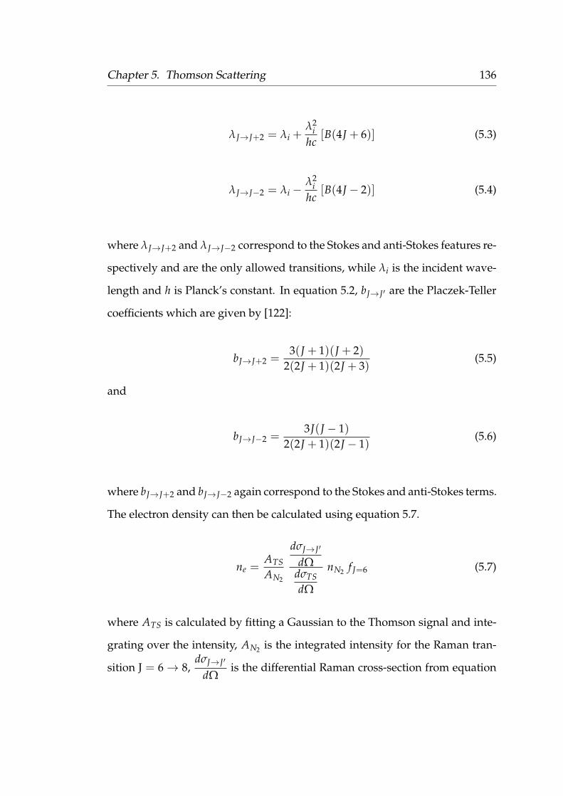
Chapter 5. Thomson Scattering 136
λJ→J+2 = λi +λ2
ihc
[B(4J + 6)] (5.3)
λJ→J−2 = λi −λ2
ihc
[B(4J − 2)] (5.4)
where λJ→J+2 and λJ→J−2 correspond to the Stokes and anti-Stokes features re-
spectively and are the only allowed transitions, while λi is the incident wave-
length and h is Planck’s constant. In equation 5.2, bJ→J′ are the Placzek-Teller
coefficients which are given by [122]:
bJ→J+2 =3(J + 1)(J + 2)
2(2J + 1)(2J + 3)(5.5)
and
bJ→J−2 =3J(J − 1)
2(2J + 1)(2J − 1)(5.6)
where bJ→J+2 and bJ→J−2 again correspond to the Stokes and anti-Stokes terms.
The electron density can then be calculated using equation 5.7.
ne =ATS
AN2
dσJ→J′
dΩdσTS
dΩ
nN2 f J=6 (5.7)
where ATS is calculated by fitting a Gaussian to the Thomson signal and inte-
grating over the intensity, AN2 is the integrated intensity for the Raman tran-
sition J = 6→ 8,dσJ→J′
dΩis the differential Raman cross-section from equation

Chapter 5. Thomson Scattering 137
5.2, whiledσTS
dΩis the differential Thomson scattering cross-section. The ni-
trogen density is given by nN2 , while f J=6 is calculated using the rigid-rotor
approximation and corresponds to the population of the J = 6 rotational level.
Once a Gaussian has been fitted to the Thomson data, the half-width half max-
imum (HWHM), ∆λ 12, can be used to calculate the corresponding electron tem-
perature, Te,
Te =mec2
8ln(2)kB sin2(θ/2)
(∆λ 1
2
λi
)2
(5.8)
where kB is the Boltzmann constant, θ is the scattering angle which in this
case is 90, λ 12
is the HWHM of the Thomson spectrum and λi is the incident
wavelength [123].
5.4.2 Results from model
Initially, by setting the electron density to zero, the model is fitted to only the
Raman data. Fitting parameters used include; the gas rotational temperature,
the percentage of nitrogen in the air, the scaling of the Raman and Rayleigh
signals and the instrument function. Figure 5.14 shows a good fit between the
model and the Raman experimental data, while figure 5.15 shows an example
of how introducing Thomson scattering affects the signal. It causes an increase
in the Raman signal intensity around 532 nm and this is clear from the change
in the Raman model (red dashed line). The example shown is for an electron
density of ne = 5× 1014 cm−3 and an electron temperature of Te = 0.3 eV.

Chapter 5. Thomson Scattering 138
FIGURE 5.14: Raman scattering experimental data (black line) asshown in figure 5.6 with fitted Raman model (red dotted line).
FIGURE 5.15: Raman scattering in air experimental data (blackline) with fitted Raman model (red dotted line) and an exampleof the Thomson signal using the model (blue line).(ne = 5× 1014 cm−3, Te = 0.3 eV.)

Chapter 5. Thomson Scattering 139
5.4.3 Electron density detection limit
No evidence of Thomson scattering was observed experimentally. However,
using the model it was possible to put an upper limit on the electron density
of the plasma, as above this limit it would have been detectable by the system.
Initially the noise level was estimated from the data, as the Thomson signal
would have to be at a greater intensity to be observed. If we take figure 5.12b
as an example, the residuals were calculated by subtracting the background
data from the signal data and then a moving 10 point standard deviation was
calculated, essentially a measure of the noise in the system. The noise level
at 531.5 nm and 532.5 nm, both regions away from the Rayleigh block, was
approximately 6800 counts.
For the Thomson signal to be observable it should have a signal-to-noise
ratio of > 1. Using the Raman model, an estimate of the electron density re-
quired for a Thomson signal level of > 7000 counts at 531.5 nm and 532.5 nm
could be obtained. Assuming an electron temperature of 0.3 eV, the electron
density required was ne = 9.95× 1012 cm−3. The Thomson profile for these pa-
rameters is shown on figure 5.16 along with data from figure 5.12b. This result
suggests that the electron density of the plasma jet in question is < 9.95× 10¹²
cm−3, as above this the experimental system would be capable of detecting it.

Chapter 5. Thomson Scattering 140
FIGURE 5.16: Thomson scattering profile of lowest detectableelectron density by the current set-up.
The closest comparison to this experiment in the literature is by Hübner et
al. [107] who were successful in observing Thomson scattering from a DBD
plasma jet, also using helium gas and running at 7 kV and 20 kHz. The elec-
tron density of this jet was found to be ne = 5× 1012 cm−3, lower than what the
experimental system in this investigation would be capable of detecting. This
electron density, ne = 5× 1012 cm−3, is the lower limit that Thomson scattering
is capable of measuring [66, 124], due to the limitations caused by stray light
and the higher intensity of the Rayleigh signal. However, Hübner et al. used
a triple grating spectrometer which would be capable of removing more of the
stray light from the system and would allow lower intensity Thomson scatter-
ing signals to be detected. Thomson scattering has been successful in many
other plasma jet systems. For example, Carbone et al. were able to measure
electron densities as low as ne = 1× 1012 cm−3, however this setup included
a triple grating spectrometer, a radio-frequency (RF) power supply and had

Chapter 5. Thomson Scattering 141
argon gas in place of helium. Other examples of using argon instead of he-
lium to achieve higher electron densities can be found in the literature [66, 106,
125], while some have measured densities on the order of ×1014 cm−3 using
microwave plasma jets [66, 126].
5.5 Summary
Unfortunately, it was not possible to observe a Thomson scattering signal for
this plasma jet. It is evident that the system is aligned spatially, as shown by
images of the laser position in the jet in figure 5.1 and by the image of Raman
scattering with helium flowing in figure 5.7, and is timed effectively. Steps
were also taken to ensure that the stray light was reduced and that the sys-
tem was stable and reproducible over time. However, using a Raman model it
was possible to put a limit on the detection capabilities of the system. Results
have shown that it would not be possible to detect Thomson scattering from
a plasma with an electron density < 9.95× 1012 cm−3. This leads to the con-
clusion that the plasma jet in this case has an electron density lower than this
threshold.

142
Chapter 6
Conclusions and Future Work
This thesis has characterised a low temperature atmospheric pressure plasma
jet using optical diagnositcs. The parameters of the jet investigated included
the electron temperature and electron density, knowledge of which is valuable
in order to control the plasma jet for various applications. Plasma imaging
and emission spectroscopy were used to obtain an understanding of the cre-
ation and propagation of the plasma both temporally and spatially. A Thom-
son scattering set-up was also used in an attempt to obtain electron density
estimates, however, with this seeming impossible due to the low density of the
plasma being studied, an upper detection limit was instead put on the system.

Chapter 6. Conclusions and Future Work 143
6.1 Conclusions
Imaging on a nanosecond timescale showed that the plasma consisted of plasma
bullets travelling at velocites on the order of 105 m s−1 which was compara-
ble to other studies on similar plasma jets. These high velocities could be at-
tributed to a photo-ionisation theory by Dawson and Winn [48], as described
in section 1.4. The plasma bullet velocity increased with applied voltage, as
you would expect, but coupled to the fact that the bullet velocities are orders
of magnitude greater than the gas flow rate, this is evidence that the plasma
is electrically driven. This is not to say that the gas flow does not contribute,
as it is essential to not only ignite the plasma, but also to allow the propaga-
tion of the plasma jet into ambient air. The acceleration of the plasma bullets
was clear in the trend of the velocity as it increased to a maximum before de-
creasing as the plasma dissipated. This can be attributed to the helium gas
as its metastable states can ionise the nitrogen from the surrounding air as it
diffuses into the plume [54, 88].
2D monochromatic imaging was used to investigate the density of excited
states which were estimated to be in the region of 1× 109 cm−3 and 2× 10¹⁰
cm−3. Along the length of the plasma plume the density of states followed
the same trend as the plasma bullet velocity. There was an initial increase in
density as the bullets propagated away from the quartz tube before a decrease.
This suggests that the brightness and velocity of the bullets are connected.
Optical emission spectroscopy identified the main chemical species in the
plasma. It was dominated by helium emission between the electrodes, while
nitrogen dominated in the plasma plume in ambient air. This may also be
attributed to the nitrogen diffusing into the plume and being ionised by helium
metastable states at the exit of the quartz tube, as discussed for the acceleration

Chapter 6. Conclusions and Future Work 144
of the plasma bullets. From this it can be concluded that the ionisation of the
nitrogen makes an important contribution the the propagation of the plasma
bullets in ambient air. The trend in the line intensity of each species along the
plasma jet axis was consistent with the trend observed in the plasma bullet
acceleration and the density of states. From this it can be concluded that the
brightest part of the plume, or where species are most densely populated, is
also where the plasma bullet velocity is greatest.
An estimate of the electron temperature was calculated using helium line
ratios, while the gas temperature was determined by analysing nitrogen emis-
sion. The electron temperature of 0.31 eV is high enough to have an effect
on biological matter, as shown by the work undertaken by the Pharmacy de-
partment at Queen’s [34–39] using this plasma jet, while the gas temperature,
estimated as 303 K, is low enough to be used in plasma medicine applications
as discussed in chapter 1.
Although the emission from the allowed and forbidden helium lines at
wavelengths of 447 nm and 492 nm are often used to estimate the electron
density [114, 116], this was not possible in this case. Due to the low electron
density of the plasma in question the methods used in other studies, at much
higher electron densities, were not applicable. However, these results were
able to be utilised in order to estimate the electric field present. Two methods,
using a graph showing the separation between the components and using an
equation, both developed by Cvetanovic et al. [117], were used and both re-
sulted in an electric field of 32.1± 1.0 kV cm−1. This showed the consistency
and reliability of the method and also agreed with other studies using similar
plasma jets [118].
The electron density of the plasma was too low to detect using Thomson

Chapter 6. Conclusions and Future Work 145
scattering as a diagnostic. Every effort was made to ensure the experimen-
tal system was capable of detecting Thomson scattering, including ensuring it
was aligned spatially, that the laser, jet and ICCD camera were synchronised
effectively and that all stray light entering the system was reduced. It was
possible, however, to put a detection limit on the capability of the system us-
ing the data obtained from the Raman scattering and modelling the level of
Thomson scattering that would be expected. It was established that the low-
est electron density detectable by the system, at an electron temperature of 0.3
eV, was 9.95× 1012 cm−3. This implies that the electron density of the plasma
investigated is below this limit.
Therefore, the main conclusions which can be drawn from this characteri-
sation of a low temperature plasma jet are that the plasma consists of plasma
bullets travelling at high velocities, much greater than the gas flow rate indi-
cating that the applied voltage is the main driving force behind the plasma.
Also, the plasma chemistry between the helium gas and the species present in
the ambient air plays an important role in the plasma propagation. Estimates
of the gas temperature and electron temperature were obtained, while the elec-
tric field was confirmed and showed that this jet has the potential to be used
effectively in the medical applications discussed in section 1.3.1. The detection
limit of the system was also established considering that Thomson scattering
could not be applied successfully.

Chapter 6. Conclusions and Future Work 146
6.2 Future work
Future work on this research should have the aim of measuring Thomson scat-
tering, however, the initial objective should be testing the validity of the set-up
i.e. achieve Thomson scattering using this experimental set-up in some way,
therefore validating the detection limit put on the system in chapter 5.
For example, a radio frequency (RF) driven plasma could be used as they
can achieve higher frequencies and in previous studies have been shown to
achieve higher electron densities on the order of 1014 cm−3 [61, 127]. Using
argon as the discharge gas instead of helium is also a possibility as this has
also been shown to increase the electron density of the plasma [61]. Both of
these changes would allow the experimental set-up to be tested and prove that
the electron density of the plasma discussed in this work was simply too low
to detect.
Replacing the GCR laser, running at 10 Hz, with a kHz laser may also in-
crease the chances of obtaining Thomson scattering. However, at higher prob-
ing intensities heating of the plasma may occur via inverse bremsstrahlung,
therefore perturbing the plasma. This must be considered before using a laser
of higher power.
A more in depth study of the plasma jet in a vertical orientation could be
carried out in order to investigate the effects of orientation on parameters other
than bullet velocity. This orientation would also allow more diagnostics to be
placed around the plasma jet to obtain data on multiple parameters simultane-
ously. Also, as mentioned in section 3.3.2, an investigation into the effect of the
cable length would help to bring to a conclusion the discussion on whether ori-
entation was the sole factor affecting the bullet velocity or whether the length
of cable between the power supply and the electrodes was also an influence.

Chapter 6. Conclusions and Future Work 147
Many of the studies which have successfully deployed Thomson scattering
as a diagnostic have used a triple grating spectrometer instead of a double
grating spectrometer [61, 63, 107, 128, 129]. Research into using a triple grating
spectrometer to resolve the issue with the low Thomson signal has already
been carried out and the process of building the spectrometer has begun. The
design is based on similar setups previously used by Kono et. al [130] and
others in the field [61, 63, 122]. A simple schematic of how it will look is shown
in figure 6.1.
FIGURE 6.1: Schematic of triple grating spectrometer setup
The introduction of an intermediate slit and a third grating allows the first
two gratings to act as a notch filter to remove the central wavelength. The
intermediate slit then removes any stray light still in the system, before the
third grating resolves the spectral information and the image is formed on the
ICCD camera. If Thomson scattering was achieved in this way it would deliver
more accurate results for the electron temperature than have been achieved

Chapter 6. Conclusions and Future Work 148
using emission spectroscopy, while also providing spatial resolution without
the need for techniques such as Abel inversion.

149
Appendix A
Other Work
Experiments contributed to:
• Sept / Oct 2015 - RAL, Vulcan (TAW) - K-edge shift under different plasma
environments.
• Aug / Sept 2016 - RAL, Vulcan (TAW) - Novel VULCAN experiments to
produce high photoionisation parameter plasmas: recreating a Seyfert galaxy in
the laboratory.
• Jan / Feb 2017 - RAL, Vulcan (TAW) - XUV Probing of Warm Dense Matter.
• June / July 2017 - RAL, Vulcan (TAW) - K-edge shifts for shock compressed
matter.

150
Appendix B
Publications related to other work
• R. Irwin, S. White, J. R. Warwick, G. Sarri, D. Riley & F. Keenan, "Study of
Ar Photoionisation Physics using VULCAN", Conference Proceedings, EPS
Conference on Plasma Physics (2017).
• S. White, R. Irwin, J. R. Warwick, G. Gribakin, G. Sarri, F. Keenan & D.
Riley, "Production of photoionized plasmas in the laboratory using x-ray line
radiation", Physical Review E. 97, 6 p. 063203 (2018).
• F. V. Brozas, C. Hyland, S. White, S. Warnock, R. Irwin, J. Campbell & D.
Riley, "Using a commercial mini-X-ray source for calibrating Bragg crystals",
Journal of Instrumentation. 13, 12, P12004 (2018).

151
Bibliography
1. Merche, D., Vandencasteele, N. & Reniers, F. Atmospheric plasmas for
thin film deposition: A critical review. Thin Solid Films 520, 4219–4236
(2012).
2. Langmuir, I. Oscillations in Ionised Gases 1928.
3. Fridman, A. & Kennedy, L. A. Plasma Physics and Engineering 2nd Ed.
(Taylor and Francis Group, 2011).
4. Chen, F. F. Introduction to Plasma Physics and Controlled Fusion 3rd Ed.
(Springer, 2016).
5. Delserieys, A. Optical diagnostics of laser plasmas PhD thesis (Queen’s Uni-
versity Belfast, 2001).
6. Delserieys, A. et al. Raman satellites in optical scattering from a laser-
ablated Mg plume. Physical Review A - Atomic, Molecular, and Optical
Physics 78, 1–4 (2008).
7. Fridman, A., Chirokov, A. & Gutsol, A. Non-thermal atmospheric pres-
sure discharges. Journal of Physics D: Applied Physics 38 (2005).
8. Algwari, Q. T. Plasma Jet Formation and Interactions between Atmospheric
Pressure Dielectric Barrier Discharge Jets PhD thesis (Queen’s University
Belfast, 2011).

BIBLIOGRAPHY 152
9. Bruggeman, P. J., Iza, F. & Brandenburg, R. Foundations of atmospheric
pressure non-equilibrium plasmas. Plasma Sources Science and Technology
26 (2017).
10. Van Gessel, B. Laser diagnostics on atmospheric pressure plasma jets PhD
thesis (Eindhoven University, 2013).
11. Robotis, J, Sechopoulos, P & Rokkas, T. Argon plasma coagulation: Clin-
ical applications in Gastroenterology. Annals of Gastroenterology 16, 131–
137 (2003).
12. Hirst, A. M., Frame, F. M., Arya, M., Maitland, N. J. & O’Connell, D. Low
temperature plasmas as emerging cancer therapeutics: the state of play
and thoughts for the future. Tumor Biology 37, 7021–7031 (2016).
13. Hirst, D. & Robson, T. Targeting nitric oxide for cancer therapy. Journal
of Pharmacy and Pharmacology 59, 3–13 (2007).
14. Laroussi, M., Kong, M. G., Morfill, G. & Stolz, W. Plasma Medicine - Ap-
plications of Low-Temperature Gas Plasmas in Medicine and Biology (Cam-
bridge University Press, 2012).
15. Laroussi, M. & Lu, X. Room-temperature atmospheric pressure plasma
plume for biomedical applications. Applied Physics Letters 87 (2005).
16. Laroussi, M., Lu, X. & Keidar, M. Perspective: The physics, diagnos-
tics, and applications of atmospheric pressure low temperature plasma
sources used in plasma medicine. Journal of Applied Physics 122 (2017).
17. Rossi, F., Kylian, O., Rauscher, H., Hasiwa, M. & Gilliland, D. Low pres-
sure plasma discharges for the sterilization and decontamination of sur-
faces. New Journal of Physics 11 (2009).
BIBLIOGRAPHY 153
18. Kong, M. G. et al. Plasma medicine: an introductory review. New Journal
of Physics 11 (2009).
19. Laroussi, M. Low-Temperature Plasmas for Medicine? IEEE Transactions
on Plasma Science 37 (2009).
20. Ehlbeck, J. et al. Low temperature atmospheric pressure plasma sources
for microbial decontamination. Journal of Physics D: Applied Physics 44
(2010).
21. Nosenko, T., Shimizu, T. & Morfill, G. E. Designing plasmas for chronic
wound disinfection. New Journal of Physics 11 (2009).
22. Fridman, G. et al. Applied Plasma Medicine. Plasma Processors and Poly-
mers (2008).
23. Graves, D. B. Low temperature plasma biomedicine: A tutorial review.
Physics of Plasmas 21 (2014).
24. Hirst, A. M., Frame, F. M., Maitland, N. J. & O’Connell, D. Low Tem-
perature Plasma Causes Double-Strand Break DNA Damage in Primary
Epithelial Cells Cultured From a Human Prostate Tumor. IEEE Transac-
tions on Plasma Science 42 (2014).
25. Stoffels, E. Biomedical applications of electric gas discharges. High Temp.
Mater. Process. 6 (2002).
26. Laroussi, M. Nonthermal Decontamination of Biological Media by Atmospheric-
Pressure Plasmas: Review, Analysis, and Prospects. IEEE Transactions on
Plasma Science 30 (2002).
27. Deng, X. T., Shi, J. J. & Kong, M. G. Protein destruction by a helium at-
mospheric pressure glow discharge: Capability and mechanisms. Journal
of Applied Physics 101 (2007).

BIBLIOGRAPHY 154
28. Keidar, M. et al. Cold atmospheric plasma in cancer therapy. Physics of
Plasmas 20 (2013).
29. O’Connell, D. et al. Cold atmospheric pressure plasma jet interactions
with plasmid DNA. Applied Physics Letters 98, 043701 (2011).
30. Sousa, J. S. et al. Cold atmospheric pressure plasma jets as sources of sin-
glet delta oxygen for biomedical applications. Journal of Applied Physics
109 (2011).
31. Noeske, M., Degenhardt, J., Strudthoff, S. & Lommatzsch, U. Plasma jet
treatment of five polymers at atmospheric pressure: surface modifica-
tions and the relevance for adhesion. International Journal of Adhesion &
Adhesives 24, 171–177 (2004).
32. Girard-Lauriault, P. L. et al. Atmospheric Pressure Deposition of Mi-
cropatterned Nitrogen-Rich Plasma-Polymer Films for Tissue Engineer-
ing. Plasma Processors and Polymers (2005).
33. Chen, C. K., Perry, W. L., Xu, H., Jiang, Y. & Phillips, J. Plasma torch pro-
duction of macroscopic carbon nanotube structures. Carbon 41, 5 (2003).
34. Flynn, P. B. et al. Bactericidal efficacy of atmospheric pressure non-thermal
plasma (APNTP) against the ESKAPE pathogens. International Journal of
Antimicrobial Agents 46, 101–107 (2015).
35. Flynn, P. B., Graham, W. G. & Gilmore, B. F. Acinetobacter baumannii
biofilm biomass mediates tolerance to cold plasma. Letters in Applied Mi-
crobiology 68, 344–349 (2019).
36. Barakat, M. M. et al. Atmospheric pressure non-thermal plasma expo-
sure reduces Pseudomonas aeruginosa lipopolysaccharide toxicity in vitro
and in vivo. Microbial Pathogenesis 136, 103679 (2019).

BIBLIOGRAPHY 155
37. Alkawareek, M. Y. et al. Eradication of Pseudomonas aeruginosa Biofilms
by Atmospheric Pressure Non-Thermal Plasma. PLoS ONE 7, 1–8 (2012).
38. Alkawareek, M. Y. et al. Application of atmospheric pressure nonthermal
plasma for the in vitro eradication of bacterial biofilms. FEMS Immunol-
ogy and Medical Microbiology 65, 381–384 (2012).
39. Gilmore, B. F. et al. Cold Plasmas for Biofilm Control: Opportunities and
Challenges. Trends in Biotechnology 36, 627–638 (2018).
40. Alkawareek, M. Y. et al. Plasmid DNA damage following exposure to at-
mospheric pressure nonthermal plasma: Kinetics and influence of oxy-
gen admixture. Plasma Medicine 4, 211–219 (2014).
41. Wielogorska, E. et al. A holistic study to understand the detoxification
of mycotoxins in maize and impact on its molecular integrity using cold
atmospheric plasma treatment. Food Chemistry 301, 125281 (2019).
42. Walsh, J. L., Iza, F., Janson, N. B., Law, V. J. & Kong, M. G. Three distinct
modes in a cold atmospheric pressure plasma jet. Journal of Physics D:
Applied Physics 43 (2010).
43. Fridman, A. Plasma Chemistry (Cambridge University Press, 2008).
44. Radmilovic-Radjenovic, M., Radjenovic, B., Klas, M., Bojarov, A. & Mate-
jcik. The breakdown mechanisms in electrical discharges: The role of the
field emission effect in direct current discharges in microgaps. Acta Phys-
ica Slovaca 63, 105–205 (2013).
45. Loeb, L. B. & Meek, J. M. The Mechanism of Spark Discharge in Air at
Atmospheric Pressure. I. Journal of Applied Physics 11 (1940).
46. Raether, H. Electron Avalanches and Breakdown in Gases (Butterworths,
1964).
BIBLIOGRAPHY 156
47. Meek, J. M. & Craggs, J. D. Electrical Breakdown of Gases (Wiley, 1978).
48. Dawson, G. A. & Winn, W. P. A model for streamer propagation. Z.
Physik 183 (1965).
49. Mericam-Bourdet, N., Laroussi, M., Begum, A. & Karakas, E. Exper-
imental investigations of plasma bullets. Journal of Physics D: Applied
Physics 42 (2009).
50. Lu, X. & Laroussi, M. Dynamics of an atmospheric pressure plasma plume
generated by submicrosecond voltage pulses. Journal of Applied Physics
(2006).
51. Shao, T. et al. Temporal evolution of atmosphere pressure plasma jets
driven by microsecond pulses with positive and negative polarities. Eu-
rophysics Letters 107 (2014).
52. Karakas, E. & Laroussi, M. Experimental studies on the plasma bullet
propagation and its inhibition. Journal of Applied Physics 108 (2010).
53. Teschke, M, Kedzierski, J, Korzec, D & Engemann, J. High-Speed Pho-
tographs of a Dielectric Barrier Atmospheric Pressure Plasma Jet. IEEE
Transactions on Plasma Science 33, 310–311 (2005).
54. Begum, A., Laroussi, M. & Pervez, M. R. Atmospheric pressure He-air
plasma jet: Breakdown process and propagation phenomenon. AIP Ad-
vances 3 (2013).
55. Shi, J., Zhong, F. & Zhang, J. A hypersonic plasma bullet train travelling
in an atmospheric dielectric-barrier discharge jet. Physics of Plasmas 15
(2008).
56. Böhle, A. et al. Pulsed discharges produced by high-power surface waves.
Journal of Physics D: Applied Physics 29 (1996).

BIBLIOGRAPHY 157
57. Brok, W. J. M., van Dijk, J., Bowden, M. D., van der Mullen, J. J.A. M. &
Kroesen, G. M. W. A model study of propagation of the first ionisation
wave during breakdown in a straight tube containing argon. Journal of
Physics D: Applied Physics 36 (2003).
58. Warner, K. & Hieftje, G. M. Thomson scattering from analytical plasmas.
Spectrochimica Acta - Part B Atomic Spectroscopy 57, 201–241 (2002).
59. Kempkens, H. & Uhlenbusch, J. Scattering diagnostics of low-temperature
plasmas (Rayleigh scattering, Thomson scattering, CARS). Plasma Sources
Science and Technology 9 (2000).
60. Muraoka, K., Uchino, K. & Bowden, M. D. Diagnostics of low-density
glow discharge plasmas using Thomson scattering. Plasma Physics and
Controlled Fusion 40 (1998).
61. Hübner, S., Sousa, J., Mullen, J. J.A.M.V. D. & Graham, W. Thomson scat-
tering on non-thermal atmospheric pressure plasma jets. Plasma Sources
Science and Technology (2015).
62. Salpeter, E. E. Electron Density Fluctuations in a Plasma. Physical Review
120 (1960).
63. Carbone, E. & Nijdam, S. Thomson scattering on non-equilibrium low
density plasmas: principles, practice and challenges. Plasma Physics and
Controlled Fusion 57 (2015).
64. Nedanovska, E. Thomson Scattering from Technological Plasmas PhD thesis
(Queen’s University Belfast, 2012).
65. Hollas, J. M. Modern Spectroscopy 4th Ed. (Wiley, 2003).

BIBLIOGRAPHY 158
66. Van Gessel, A. F. H., Carbone, E. A. D., Bruggeman, P. J. & van der
Mullen, J. J.A. M. Laser scattering on an atmospheric pressure plasma
jet : disentangling Rayleigh , Raman and Thomson scattering. Plasma
Sources Science and Technology (2012).
67. Tektronix. P6015A Instruction Manual <www.tektronix.com>.
68. PearsonElectronics. Pearson Current Monitor Model 2877 Spec Sheet 1999.
<pearsonelectronics.com/products/wideband-current-monitors>.
69. PearsonElectronics. Pearson Current Monitor Model 2878 Spec Sheet 1999.
<pearsonelectronics.com/products/wideband-current-monitors>.
70. Rott, N. Note on the history of Reynolds number. Annual Review of Fluid
Mechanics 22, 1–11 (1990).
71. Niemi, K., Waskoenig, J., Sadeghi, N., Gans, T. & O’Connell, D. The role
of helium metastable states in radio-frequency driven helium-oxygen at-
mospheric pressure plasma jets: measurement and numerical solution.
Plasma Sources Science and Technology 20 (2011).
72. Hyperphysics. Helium energy levels <http://hyperphysics.phy-astr.
gsu.edu/hbase/quantum/helium.html> (visited on 01/19/2020).
73. Flynn, P. B. et al. Non-thermal plasma exposure rapidly attenuates bac-
terial AHL-dependent quorum sensing and virulence. Scientific Reports
6, 18–30 (2016).
74. Knake, N., Niemi, K., Reuter, S., Schulz-Von Der Gathen, V. & Winter, J.
Absolute atomic oxygen density profiles in the discharge core of a mi-
croscale atmospheric pressure plasma jet. Applied Physics Letters 93, 16–
19 (2008).

BIBLIOGRAPHY 159
75. Knake, N., Reuter, S., Niemi, K., Schulz-Von Der Gathen, V. & Winter,
J. Absolute atomic oxygen density distributions in the effluent of a mi-
croscale atmospheric pressure plasma jet. Journal of Physics D: Applied
Physics 41 (2008).
76. Goree, J., Liu, B. & Drake, D. Gas flow dependence for plasma-needle
disinfection of S. mutans bacteria. Journal of Physics D: Applied Physics 39,
3479–3486 (2006).
77. Andor Technology. iStar CCD User Manual 1.1 tech. rep. (2012).
78. Bruggeman, P. J., Sadeghi, N., Schram, D. C. & Linss, V. Gas tempera-
ture determination from rotational lines in non-equilibrium plasmas: a
review. Plasma Sources Science and Technology 23 (2014).
79. Bowden, M. D. et al. A Thomson scattering diagnostic system for mea-
surement of electron properties of processing plasmas. Plasma Sources
Science and Technology 8, 203–209 (1999).
80. Röhr, H., Steuer, K. H., Schramm, G., Hirsch, K. & Salzmann, H. First
high-repetition-rate Thomson scattering for fusion plasmas. Nuclear Fu-
sion 22, 1099–1102 (1982).
81. Bowden, M. D. et al. Comparison of electron property measurements
in an inductively coupled plasma made by Langmuir probe and laser
Thomson scattering techniques. Journal of Vacuum Science & Technology A
17 (1999).
82. Bakker, L. P., Freriks, J. M., de Hoog, F. J. & Kroesen, G. M. W. Thomson
scattering using an atomic notch filter. Review of Scientific Instruments 71
(2000).

BIBLIOGRAPHY 160
83. Nedanovska, E. et al. Comparison of the electron density measurements
using Thomson scattering and emission spectroscopy for laser induced
breakdown in one atmosphere of helium. Applied Physics Letters 99, 2013–
2016 (2011).
84. Nedanovska, E. et al. Investigating the dynamics of laser induced sparks
in atmospheric helium using Rayleigh and Thomson scattering. Journal
of Applied Physics 117 (2015).
85. Jiang, N., Ailing, J. & Cao, Z. Atmospheric pressure plasma jet: Effect of
electrode configuration, discharge behaviour, and its formation mecha-
nism. Journal of Applied Physics 106 (2009).
86. Xiong, Z. et al. Measurements of the Propagation Velocity of an Atmospheric-
Pressure Plasma Plume by Various Methods. IEEE Transactions on Plasma
Science 38 (2010).
87. Lu, X., Laroussi, M. & Puech, V. On atmospheric-pressure non-equilibrium
plasma jets and plasma bullets. Plasma Sources Science and Technology 21
(2012).
88. Wu, S., Huang, Q., Wang, Z. & Lu, X. The effect of nitrogen diffusion
from surrounding air on plasma bullet behavior. IEEE Transactions on
Plasma Science 39, 2286–2287 (2011).
89. Jonkers, J., Selen, L. J. M., van der Mullen, J. A. M., Timmermans, E. A. H.
& Schram, D. C. Steep plasma gradients studied with spatially resolved
Thomson scattering measurements. Plasma Sources Science and Technology
6 (1997).

BIBLIOGRAPHY 161
90. De Regt, J. M., de Groote, F. P. J., van der Mullen, J. A. M. & Schram, D. C.
Air entrainment in an inductively coupled plasma measured by Raman
and Rayleigh scattering. Spectrochimica Acta Part B (1996).
91. Álvarez, R., Rodero, A. & Quintero, M. C. An Abel inversion method for
radially resolved measurements in the axial injection torch. Spectrochim-
ica Acta - Part B Atomic Spectroscopy 57, 1665–1680 (2002).
92. Engel, U., Prokisch, C., Voges, E., Hieftje, G. M. & Broekaert, J. A. Spa-
tially resolved measurements and plasma tomography with respect to
the rotational temperatures for a microwave plasma torch. Journal of An-
alytical Atomic Spectrometry 13, 955–961 (1998).
93. Nestor, O. H. & Olsen, H. N. Numerical Methods for Reducing Line and
Surface Probe Data. SIAM Review 2 (1960).
94. Kelsey, C. Characterisation of Plasmas Produced in Vapour Layers in Con-
ducting Solutions PhD thesis (2014).
95. NIST Atomic Spectra Database Lines <https : / / physics . nist . gov /
PhysRefData/ASD/lines\_form.html>.
96. Sakiyama, Y., Graves, D. B., Jarrige, J. & Laroussi, M. Finite element anal-
ysis of ring-shaped emission profile in plasma bullet. Applied Physics Let-
ters 96, 1–4 (2010).
97. Naidis, G. V. Modelling of plasma bullet propagation along a helium jet
in ambient air. Journal of Physics D: Applied Physics 44 (2011).
98. Ramsey, A. T. & Diesso, M. Abel inversions: Error propagation and in-
version reliability. Review of Scientific Instruments 70 (1999).
99. Loureiro, J. & Amorim, J. Kinetics and Spectroscopy of Low Temperature
Plasmas (Springer, 2016).

BIBLIOGRAPHY 162
100. Griem, H. R. Principles of Plasma Spectroscopy (Cambridge University Press,
1997).
101. Tendero, C., Tixier, C., Tristant, P., Desmaison, J. & Leprince, P. Atmo-
spheric pressure plasmas: A review. Spectrochimica Acta - Part B Atomic
Spectroscopy 61, 2–30 (2006).
102. Kunze, H. J. Introduction to Plasma Spectroscopy (Springer, 2009).
103. Fujimoto, T. & McWhirter, R. W. Validity criteria for local thermody-
namic equilibrium in plasma spectroscopy. Physical Review A 42, 6588–
6601 (1990).
104. Hutchinson, I. H. Principles of Plasma Diagnostics 1st Ed. (1987).
105. Podder, N. K. et al. Helium line intensity ratio in microwave-generated
plasmas. Physics of Plasmas 11, 5436–5443 (2004).
106. Belostotskiy, S. G. et al. Measurement of electron temperature and den-
sity in an argon microdischarge by laser Thomson scattering. Applied
Physics Letters 92 (2008).
107. Hübner, S., Sousa, J. S., Puech, V., Kroesen, G. M. & Sadeghi, N. Electron
properties in an atmospheric helium plasma jet determined by Thomson
scattering. Journal of Physics D: Applied Physics 47 (2014).
108. Mihalas, D., Cooper, J & Smith, E. W. He I 4471 Profiles In B Stars: Calcu-
lations With An Improved Line-Broadening Theory. Astrophysical Journal
190, 315–318 (1974).
109. Monfared, S. K., Graham, W. G., Morgan, T. J. & Hüwel, L. Spectro-
scopic characterization of laser-produced atmospheric pressure helium
microplasmas. Plasma Sources Science and Technology 20 (2011).

BIBLIOGRAPHY 163
110. Adler, H. G. & Piel, A. Stark-broadening of the helium lines 447 and
492 nm at low electron densities. Journal of Quantitative Spectroscopy and
Radiative Transfer 45, 11–31 (1991).
111. Obradovic, B. M., Ivkovic, S. S. & Kuraica, M. M. Spectroscopic measure-
ment of electric field in dielectric barrier discharge in helium. Applied
Physics Letters 92 (2008).
112. Allen, D. in Exercises in Astronomy (Springer, 1987).
113. Milosavljevic, V. On the Stark broadening of the He I 447 . 1 nm spectral
line. European Physical Journal D 104, 99–104 (2001).
114. Pérez, C., De La Rosa, I., Aparicio, J. A., Mar, S. & Gigosos, M. A. Calibra-
tion of the stark-broadening parameters of two He I lines with forbidden
components. Japanese Journal of Applied Physics, Part 1: Regular Papers and
Short Notes and Review Papers 35, 4073–4076 (1996).
115. Moore, C. E. Atomic Energy Levels 1st Ed. (1949).
116. Czernichowski, A. & Chapelle, J. Use of the 447nm He I line to determine
electron concentrations. Journal of Quantitative Spectroscopy & Radiative
Transfer 33, 427–436 (1985).
117. Cvetanovic, N., Martinovic, M. M., Obradovic, B. M. & Kuraica, M. M.
Electric field measurement in gas discharges using stark shifts of He
i lines and their forbidden counterparts. Journal of Physics D: Applied
Physics 48 (2015).
118. Sretenovic, G. B., Krstic, I. B., Kovacevic, V. V., Obradovic, B. M. & Ku-
raica, M. M. Spectroscopic measurement of electric field in atmospheric-
pressure plasma jet operating in bullet mode. Applied Physics Letters 99,
10–13 (2011).

BIBLIOGRAPHY 164
119. Naidis, G. V. Modelling of streamer propagation in atmospheric-pressure
helium plasma jets. Journal of Physics D: Applied Physics 43 (2010).
120. Kuraica, M. M. & Konjevic, N. Electric field measurement in the cathode
fall region of a glow discharge in helium. Applied Physics Letters 70 (1997).
121. Obradovic, B. M. & Kuraica, M. M. On the use of relative line intensities
of forbidden and allowed components of several HeI lines for electric
field measurements. Physics Letters A (2008).
122. Van de Sande, M. Laser scattering on low temperature plasmas: High resolu-
tion and stray light rejection PhD thesis (Eindhoven, 2002).
123. Roettgen, A. et al. Time-resolved electron density and electron temper-
ature measurements in nanosecond pulse discharges in helium. Plasma
Sources Science and Technology 25 (2016).
124. Nikiforov, A. Y., Leys, C., Gonzalez, M. A. & Walsh, J. L. Electron density
measurement in atmospheric pressure plasma jets: Stark broadening of
hydrogenated and non-hydrogenated lines. Plasma Sources Science and
Technology 24 (2015).
125. Hübner, S., Hofmann, S., van Veldhuizen, E. M. & Bruggeman, P. J. Elec-
tron densities and energies of a guided argon streamer in argon and air
environments. Plasma Sources Science and Technology 22 (2013).
126. Palomares, J. M., Iordanova, E. I., Gamero, A., Sola, A. & van der Mullen,
J. J.A. M. Atmospheric microwave-induced plasmas in Ar/H2 mixtures
studied with a combination of passive and active spectroscopic methods.
Journal of Physics D: Applied Physics 43 (2010).

BIBLIOGRAPHY 165
127. Van Gessel, B., Brandenburg, R. & Bruggeman, P. Electron properties and
air mixing in radio frequency driven argon plasma jets at atmospheric
pressure. Applied Physics Letters 103, 1–5 (2013).
128. Kono, A. & Iwamoto, K. High-spatial-resolution multichannel thomson
scattering measurements for atmospheric pressure microdischarge. Japanese
Journal of Applied Physics, Part 2: Letters 43 (2004).
129. Van de Sande, M. J., Deckers, R. H., Lepkojus, F., Buscher, W. & Van der
Mullen, J. J. Time resolved electron density and temperature measure-
ments on a capacitively coupled helium RF discharge. Plasma Sources
Science and Technology 11, 466–475 (2002).
130. Kono, A. & Nakatani, K. Efficient multichannel Thomson scattering mea-
surement system for diagnostics of low-temperature plasmas. Review of
Scientific Instruments 71, 2716 (2000).