Optical Computing for Fast Light Transport Analysis

Matthew O’Toole∗ Kiriakos N. Kutulakos∗

University of Toronto

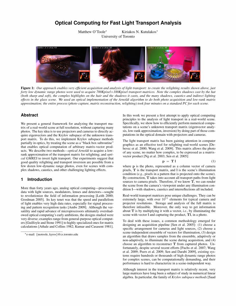
Figure 1: Our approach enables very efficient acquisition and analysis of light transport: to create the relighting results shown above, justforty low dynamic range photos were used to acquire 700Kpixel×100Kpixel transport matrices. Note the complex shadows cast by the hat(both sharp and soft), the complex highlights on the hair and the shadows it casts, and the many shadows, caustics and indirect lightingeffects in the glass scene. We used an optical implementation of the Arnoldi algorithm to do both photo acquisition and low-rank matrixapproximation; the entire process (photo capture, matrix reconstruction, relighting) took four minutes on a standard PC for each scene.

Abstract

We present a general framework for analyzing the transport ma-trix of a real-world scene at full resolution, without capturing manyphotos. The key idea is to use projectors and cameras to directly ac-quire eigenvectors and the Krylov subspace of the unknown trans-port matrix. To do this, we implement Krylov subspace methodspartially in optics, by treating the scene as a “black box subroutine”that enables optical computation of arbitrary matrix-vector prod-ucts. We describe two methods—optical Arnoldi to acquire a low-rank approximation of the transport matrix for relighting; and opti-cal GMRES to invert light transport. Our experiments suggest thatgood quality relighting and transport inversion are possible from afew dozen low-dynamic range photos, even for scenes with com-plex shadows, caustics, and other challenging lighting effects.

1 Introduction

More than forty years ago, analog optical computing—processingdata with light sources, modulators, lenses and detectors—soughtto revolutionize the field of information processing [Leith 2000;Goodman 2005]. Its key tenet was that the speed and parallelismof light enables very high data rates, especially for signal process-ing and pattern recognition tasks [Ambs 2009]. Although the ver-satility and rapid advance of microprocessors ultimately overshad-owed optical computing’s early ambitions, the designs studied werevery diverse; examples range from general-purpose optical comput-ers [Guilfoyle and Stone 1991] to highly specialized ones for matrixcalculations [Athale and Collins 1982; Kumar and Casasent 1981].

∗e-mail: {motoole, kyros}@cs.toronto.edu

In this work we present a first attempt to apply optical computingprinciples to the analysis of light transport in a real-world scene.Specifically, we show how to efficiently perform numerical compu-tations on a scene’s unknown transport matrix (eigenvector analy-sis, low-rank approximation, inversion) by doing part of those com-putations in the optical domain with projectors and cameras.

The light transport matrix has been gaining attention in computergraphics as an effective tool for relighting real-world scenes [De-bevec et al. 2000; Wang et al. 2009]. This matrix allows the photoof any scene, no matter how complex, to be expressed as a matrix-vector product [Ng et al. 2003; Sen et al. 2005]:

p = T l (1)

where p is the photo, represented as a column vector of camerapixels, T is the transport matrix, and l is the scene’s illuminationcondition (e.g., pixels in a pattern that is projected onto the scene).By construction, T takes into account all transport paths from lightsources to camera pixels. Therefore, if we know T, we can renderthe scene from the camera’s viewpoint under any illumination con-dition l—with shadows, caustics and interreflections all included.

Real-world transport matrices pose unique challenges. They can beextremely large, with over 1011 elements for typical camera andprojector resolutions. Storage and analysis of the full matrix istherefore infeasible. Moreover, the only way to get informationabout T is by multiplying it with a vector, i.e., by illuminating thescene with vector l and capturing the product, Tl, in a photo.

To deal with these issues, a common methodology emerged fordesigning an acquisition pipeline [Sen et al. 2005]: (1) choose aspecific arrangement for cameras and light sources, (2) choose ascene-independent ensemble of vectors for illumination, (3) designan algorithm that draws samples from the ensemble, adaptively ornon-adaptively, to illuminate the scene during acquisition, and (4)choose an algorithm to reconstruct T from captured photos. Un-fortunately, despite several recent efforts [Fuchs et al. 2007; Wanget al. 2009; Peers et al. 2009; Sen and Darabi 2009], existing sys-tems require hundreds or thousands of high dynamic range photosfor complex scenes, can be computationally demanding, and theirperformance is hard to characterize in a scene-independent way.

Although interest in the transport matrix is relatively recent, verylarge matrices have long been a subject of study in numerical linearalgebra. In particular, the family of Krylov subspace methods [Saad

2003] is designed for matrices just like T, i.e., very large and un-observable matrices that can only be accessed by computing theirproduct with a vector. These iterative algorithms are well under-stood and come with explicit accuracy and convergence guarantees.

Here we leverage this body of work for light transport by imple-menting Krylov subspace methods partially in optics. Our approachis based on a simple principle: treat the scene as a “black-box sub-routine” that accepts any non-negative vector l as “input” and re-turns as “output” the vector’s product, Tl, with the unknown trans-port matrix. Thus, any efficient numerical method that relies exclu-sively on matrix-vector products can be readily implemented in op-tics and used to analyze T. To do the conversion, we just replace allmatrix-vector products with calls to a function that computes themoptically, with illuminate-and-capture operations (Figure 2). Thisturns Krylov subspace methods into complete pipelines for analyz-ing T—as they pursue their numerical objective, they fully specifyhow to illuminate the scene and how to process its photos.

Implementing Krylov subspace methods directly in the optical do-main has several advantages. First, the convergence rate of thesemethods depends only on the distribution of T’s singular values,not its absolute size. This means that T can be analyzed at fullresolution by capturing very few photos. Second, computations areefficient because the only computationally-expensive step is multi-plying the full-resolution T with a vector—which we do optically.Third, optical implementations are straightforward because theydiffer from widely-available numerical software in just one step,i.e., multiplication with T. Last but not least, by moving this multi-plication to the optical domain we make other computations feasi-ble on the full-resolution T, beyond mere acquisition—computingeigenvectors of T, computing products with T’s inverse—withouthaving to acquire the transport matrix first.

We focus on optical versions of two Krylov subspace methods inthis paper: Arnoldi iteration to acquire a low-rank approximationof T for relighting (Section 3); and generalized minimal residual(GMRES) to invert light transport (Section 4). In the following weassume that illumination vectors in Equation 1 have m elementsand photos have n pixels, i.e., T is an n×m matrix.

2 Computing with Light

2.1 A Simple Example: Optical Power Iteration

We begin by showing how to implement power iteration in op-tics. Power iteration is a simple numerical algorithm for estimatingthe principal eigenvector of a square matrix with distinct eigenval-ues [Trefethen and Bau 1997]. When implemented optically, it es-timates the principal eigenvector of T without advance knowledgeof the matrix and without directly capturing any of its elements.

Power iteration uses the fact that the sequence l,Tl,T2l,T3l, . . .converges to T’s principal eigenvector for almost any initial vectorl. The algorithm simply generates this sequence for a fixed numberof iterations using the boxed matrix-vector product on the left:

Algorithm 1 The power iteration algorithm.

Numerical Implementation:

In: matrix T, iterations KOut: principal eigenvector of T

1: l1 = random vector

2: for k = 1 to K

3: pk = Tlk

4: lk+1 = pk/‖pk‖2

5: return lk+1

Optical Implementation:

In: iterations KOut: principal eigenvector of T

l1 = positive vector

for k = 1 to K

illuminate scene with vector lkcapture photo & store in pk

lk+1 = pk/‖pk‖2

return lk+1

Implementing power iteration in optics amounts to replacing thisproduct with the illuminate-and-capture operation shown on theright. This is possible when the transport matrix is square, i.e.,when illumination vectors and captured photos are the same size.

Tl computable optically Tl computable optically

T sparse, high-rank for Lambertian scene T dense, low-rank for Lambertian scene

... ...

scene

n pixels m pixels

lTl

...

scene

...

n pixels m pixels

lTl

display

screen

(a) (b)

Tl and Ttl computable optically Tl and Ttr computable optically

T symmetric T non-symmetric

...

...

scenenpix

els

n pixels

l

Tl

beamsplitter

... ...

scene

n pixels m pixels

rl

TlTtr

beamsplitter

(c) (d)

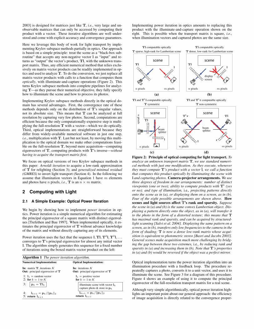
Figure 2: Principle of optical computing for light transport. Toanalyze an unknown transport matrix T, we use standard numeri-cal methods with just one modification. As they execute, wheneverthey must compute T’s product with a vector l, we call a functionthat computes this product optically by illuminating the scene withl and capturing photos. Camera-projector arrangements. We usethree degrees of freedom in our arrangements: number of distinctviewpoints (one or two); ability to compute products with Tt (yesor no); and type of illumination, i.e., projecting patterns directlyonto the scene as in (a), or displaying them on a screen, as in (b).Four of the eight possible arrangements are shown above. Howscenes and light sources affect T’s rank and sparsity. Supposethe scene in (a) and (b) is the same convex Lambertian object. Dis-playing a pattern directly onto the object, as in (a), will transfer itto the photo in the form of a distorted texture; this means that Thas maximal rank and sparsity, and can be acquired by structured-light scanning [Salvi et al. 2004]. Displaying the same pattern on ascreen, as in (b), transfers only low frequencies to the camera in theform of shading; T is now a dense low-rank matrix whose acqui-sition is equivalent to photometric stereo [Basri and Jacobs 2003].General scenes make acquisition much more challenging by bridg-ing the gap between these two extremes, i.e., by reducing rank andsparsity in (a) and increasing them in (b). Note that T’s propertiesin (a) and (b) would be reversed if the object was a perfect mirror.

Optical implementation turns the power iteration algorithm into anillumination procedure with a feedback loop. The procedure re-peatedly captures a photo, converts it to a unit vector, and uses it toilluminate the scene. See Figure 3 for a diagram of this procedure.Figure 4 shows an example of using it to compute the principaleigenvector of the full-resolution transport matrix for a real scene.

Although very simple algorithmically, optical power iteration high-lights an important point about our general approach: the efficiencyof image acquisition is directly related to the convergence proper-

illumination

pattern

captured

photo

normalize

illuminate &

capture

positive

vectorprincipal

eigenvector

l1 lk Tlk lK

Figure 3: Power iteration with a projector and a camera.

l1 l2 l3

l4 l50 l100

Figure 4: Optical power iteration in action. We used the coax-ial arrangement of Figure 2(c) for this example, where a cameraand a projector share the same viewpoint and T is symmetric. Westarted with a constant illumination vector l1, shown above, so thefirst photo of the scene was captured under constant illumination.That photo became the next illumination vector, l2, also shownabove. The illumination vectors change very little after about 50captured photos, indicating that a good approximation of T’s prin-cipal eigenvector has already been found.

ties of the underlying numerical algorithm—the faster it converges,the fewer photos its optical implementation needs to capture.

From a numerical standpoint, power iteration is not an efficient al-gorithm for computing eigenvectors. It computes just one eigenvec-tor, albeit the principal one, and the approximation error decreasesby a factor of |λ2|/|λ1| at each iteration, where λ1, λ2 are the toptwo eigenvalues of T [Trefethen and Bau 1997]. The algorithmmay converge very slowly when T’s top two eigenvalues are sim-ilar, and may not converge at all if they are identical. Naturally,these limitations are shared by its optical counterpart.

To analyze light transport efficiently, we focus on much more effi-cient numerical algorithms from the class of Krylov subspace meth-ods, discussed below.

2.2 Optical Krylov Subspace Methods

Krylov subspace methods represent some of the most importantiterative algorithms for solving large linear systems [Saad 2003].Their relevance for light transport comes from the existence ofpowerful methods for analyzing large sparse matrices, like T, beit square or rectangular, and symmetric or non-symmetric.

Briefly, the Krylov subspace of dimension k is the span of vectorsproduced by power iteration after k steps:

l1 l2 l3 · · · lk+1

m m m

Tl1 T2l1 · · · Tkl1

. (2)

While individual algorithms differ in their specifics, Krylov sub-space methods take an initial vector l1 as input and, in their k-thiteration, compute a vector in the Krylov subspace of dimension k.

The important characteristic of these methods is that they do notrequire direct access to the elements of T; all they need is the abil-ity to multiply T, and potentially its transpose, with a vector. Thismakes them readily implementable in optics.

Optical matrix-vector products for general vectors Unlikepower iteration, general Krylov subspace methods require multi-plying T with vectors that may contain negative elements. Eventhough we cannot illuminate the scene with negative light, imple-menting such products optically is straightforward. We follow theapproach outlined by Goodman [2005], and express a general vec-tor l as the difference of two non-negative vectors lp and ln:

l = lp − l

n(3)

T l = (T lp)− (T l

n) . (4)

To implement Equation 4 optically, we use two illuminate-and-capture operations: one to compute Tlp and one to compute Tln.We then subtract the two captured photos to get the product with l.

Symmetric vs. non-symmetric transport matrices The con-vergence behavior of Krylov subspace methods like GMRES de-pends quite significantly on whether or not T is a symmetric ma-trix [Liesen and Tichy 2004]. In this paper we restrict ourselvesto the symmetric case, where convergence is well understood, bychoosing appropriate projector-camera arrangements.

There are two general ways to enforce symmetry when implement-ing Krylov subspace methods in optics. The first is to make surethat T itself is symmetric. This can be done with the coaxialarrangement of Figure 2(c). This configuration takes advantageof Helmholtz reciprocity and is quite common [Seitz et al. 2005;Zhang and Nayar 2006]. It is also quite limited because it does notallow any viewpoint variations between the projector and camera.

A second way to enforce symmetry is to apply the methods to adifferent matrix whose symmetry is guaranteed:

T∗ = T

tT . (5)

Optically multiplying T∗ with a vector, however, involves matrix-vector products with both T and its transpose:

T∗

l = Tt (T l) . (6)

A single camera-projector pair is not enough to compute both prod-ucts optically. For this, we use the arrangement of Garg et al. [2006]shown in Figure 2(d). This arrangement uses two camera-projectorpairs and enables two distinct project-and-capture operations: onefor computing Tl (“illuminate from left, capture from right”) andone for computing Ttr (“illuminate from right, capture from left”).

Arnoldi and GMRES Krylov subspace methods come in manyflavors depending on the numerical objective (eigenvalue estima-tion, solution of linear systems, etc.); type of matrix (symmetric,non-symmetric, positive definite, etc.); and error tolerance. We ex-plore two of these methods here: Arnoldi iteration for efficientlyacquiring a low-rank approximation of T, and generalized minimalresidual (GMRES) for inverting light transport.

When implemented in optics, Arnoldi and GMRES follow the samebasic loop as optical power iteration. They capture a photo, processit, project the result back onto the scene, and repeat for a fixed num-ber of iterations. Both methods differ from power iteration in justthree steps. These differences are summarized in Table 1.

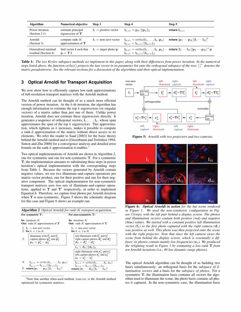
Algorithm Numerical objective Step 1 Step 4 Step 5

Power iteration estimate principal l1 = positive vector lk+1 = pk/‖pk‖2 return lk+1

(Section 2.1) eigenvector of T

Arnoldi compute rank-K l1 = non-zero vector lk+1 = ortho(l1, . . . , lk,pk) return [p1 · · ·pK ][l1 · · · lK ]t

(Section 3) approximation of T lk+1 = lk+1/‖lk+1‖2

Generalized minimal find vector l such that l1 = target photo p lk+1 = ortho(l1, . . . , lk,pk) return [l1 · · · lK ][p1 · · ·pK ]+p

residual (Section 4) p = T l lk+1 = lk+1/‖lk+1‖2

Table 1: The two Krylov subspace methods we implement in this paper, along with their differences from power iteration. In the numericalsteps listed above, the function ortho() projects the last vector in its parameter list onto the orthogonal subspace of the rest; [ ]+ denotes thematrix pseudoinverse. See the relevant sections for a discussion of the algorithms and their optical implementation.

3 Optical Arnoldi for Transport Acquisition

We now show how to efficiently capture low-rank approximationsof full-resolution transport matrices with the Arnoldi method.

The Arnoldi method can be thought of as a much more efficientversion of power iteration. At the k-th iteration, the algorithm hasenough information to estimate the top k eigenvectors (or singularvectors) of a matrix rather than just one of them. Unlike poweriteration, Arnoldi does not estimate these eigenvectors directly. Itgenerates a sequence of orthogonal vectors, l1, . . . , lk, whose spanapproximates the span of the top k eigenvectors. This approxima-tion, which tightens as k increases, makes it possible to computea rank-k approximation of the matrix without direct access to itselements. We refer the reader to Saad [2003] for the basic theorybehind the Arnoldi method and to [Greenbaum and Trefethen 1994;Simon and Zha 2000] for a convergence analysis and detailed errorbounds on the rank-k approximation it enables.1

Two optical implementations of Arnoldi are shown in Algorithm 2,one for symmetric and one for non-symmetric T. For a symmetricT, the implementation amounts to substituting three steps in poweriteration’s optical implementation with the corresponding stepsfrom Table 1. Because the vectors generated by Arnoldi containnegative values, we use two illuminate-and-capture operations permatrix-vector product, one for their positive and one for their neg-ative component. The optical implementation for non-symmetrictransport matrices uses two sets of illuminate-and-capture opera-tions, applied to T and Tt respectively, in order to implementEquation 6. Therefore, we capture four photos per Arnoldi iterationwhen T is non-symmetric. Figure 5 shows the schematic diagramfor this case and Figure 6 shows an example run.

Algorithm 2 Optical Arnoldi for rank-K transport acquisition.

For symmetric T:

In: iterations KOut: rank-K approximation of T

1: l1 = non-zero vector

2: for k = 1 to K

3:illuminate with l

p

kand lnk

capture photos pp

kand pn

k

pk = pp

k− pn

k

4: lk+1 = ortho(l1, . . . , lk,pk)lk+1 = lk+1/‖lk+1‖2

5: return [p1 · · ·pK ][l1 · · · lK ]t

For non-symmetric T:

In: iterations KOut: rank-K approximation of T

l1 = non-zero vector

for k = 1 to K

left-illuminate with lp

kand lnk

right-capture photos dp

kand dn

k

dk = dp

k− dn

k

rk = dk/‖dk‖2

right-illuminate with rp

kand rnk

left-capture photos sp

kand snk

sk = sp

k− snk

lk+1 = ortho(l1, . . . , lk, sk)lk+1 = lk+1/‖lk+1‖2

return [d1 · · ·dK ][l1 · · · lK ]t

1Note that another often-used method, Lanczos, is the Arnoldi method

optimized for symmetric matrices.

left-

illuminate

right-

capture

non-zero

vector

left-

illuminate

right-

capture

pos/neg

split

orthogonalize

left-

capture

right-

illuminate

left-

capture

right-

illuminate

pos/neg

split

normalize

l1 lp

klnk

dp

k=Tl

p

kdnk=Tln

k

rp

krnk

sp

k=Tr

p

ksnk=Trn

k

Figure 5: Arnoldi with two projectors and two cameras.

l1 l10 l40

d1 d10 d40

s1 s10 s40

Figure 6: Optical Arnoldi in action for the hat scene renderedin Figure 1. We used the non-symmetric configuration in Fig-ure 11(top), with the left pair behind a display screen. The photosand illumination vectors contain both positive (red) and negative(blue) values. We started with a constant positive left illuminationvector (l1) so the first photo captured with the right camera (d1)was positive as well. This photo was then projected onto the scenewith the right projector. Note that since the left camera views thescene from behind the display screen, which is essentially a dif-fuser, its photos contain mainly low frequencies (s1). We producedthe relighting result in Figure 1 by estimating a low-rank T fromten Arnoldi iterations (i.e., 40 low dynamic range photos).

The optical Arnoldi algorithm can be thought of as building twobases simultaneously: an orthogonal basis for the subspace of il-lumination vectors and a basis for the subspace of photos. For asymmetric T, the illumination basis contains all vectors the algo-rithm used to illuminate the scene; the photo basis contains all pho-tos it captured. In the non-symmetric case, the illumination basis

contains the left-illumination vectors (first row of Figure 6) and thephoto basis the right-captured photos (second row of Figure 6). Thematrix itself, returned in the algorithm’s last step, just multipliesthese two bases together.

Scene relighting To render a scene under a novel illuminationvector l, we rewrite Equation 1 in terms of the captured illuminationand photo bases. The equation for the non-symmetric case becomes

p = [d1 · · ·dK ][l1 · · · lK ]t l . (7)

This equation can be thought of as a two-step relighting procedure:first we compute l’s coordinates in the left-illumination basis byprojecting l onto it; then we linearly combine the right-capturedphotos to obtain the relighting result, p.

3.1 Relation to Prior Work on Transport Acquisition

We discuss related work from a numerical perspective in terms offour properties—T’s rank, sparsity, row space, and symmetry.

An important distinction between methods is the rank and sparsityof matrices they acquire. As we illustrate in Figure 2, this distinc-tion is implicit in the choice of a light source and scene. Techniquesgeared toward sparse high-rank matrices [Sen et al. 2005; Garget al. 2006; Peers and Dutre 2005] rely on T’s ability to transferboth high and low frequencies from the illumination domain to thecamera domain; techniques acquiring dense low-rank matrices [De-bevec et al. 2000; Fuchs et al. 2007; Wang et al. 2009] assume thathigh-frequency illumination does not propagate to the camera do-main. Optical Arnoldi is primarily applicable to dense low-rankmatrices. These are often representative of natural settings, whereillumination comes from point or area sources and where mirror re-flection and sharp shadows usually do not dominate light transport.

The choice of illumination ensemble used to acquire the transportmatrix is critical because it controls the basis for T’s row space. Tomaximize efficiency, this ensemble should allow accurate recon-struction of T’s rows from as few illumination vectors as possible.Many ensembles have been used for this purpose, including Haarwavelets [Peers and Dutre 2003], Hadamard patterns [Schechneret al. 2007] and single-source illuminations [Fuchs et al. 2007]. Forinstance, Wang et al. [2009] use the low-rank configuration in Fig-ure 2(b) and single-source illumination vectors to reconstruct T’srows with the kernel Nystrom method. These ensembles have beenscene independent in all previous work on transport acquisition.2

For low-rank matrices, no scene-independent ensemble is optimal.The optimal ensemble under the Frobenius norm is scene dependentand consists of T’s singular vectors [Trefethen and Bau 1997]. Thisis precisely the ensemble optical Arnoldi approximates.

Garg et al. [2006] and Wang et al. [2009] used coaxial camera-projector arrangements to exploit the fact that knowing a subsetof both rows and columns of T makes it easier to reconstruct therest. Numerically, however, symmetry has much more fundamen-tal effect on a matrix, as it affects its eigenstructure. While we usesimilar camera-projector arrangements, our choices are guided pri-marily by numerical convergence considerations.

Sen et al. [2009] and Peers et al. [2009] recently used compressedsensing techniques to reconstruct individual rows of T. Thesemethods are complementary to our own, as they apply to a dif-ferent matrix class—sparse, high-rank matrices—for which a low-rank approximation might lead to rendering artifacts. The scene-independent ensembles of these methods, however, are inefficient

2Although techniques have been proposed for sampling vectors from

within an ensemble in a scene-dependent way (e.g., [Fuchs et al. 2007]),

the ensemble itself is fixed and independent of the scene.

for capturing dense low-rank matrices. They are also very expen-sive computationally and depend on the size of T. Here, by seek-ing to maximize the “information content” of each captured photo,optical Arnoldi makes the number of iterations required for conver-gence dependent on T’s singular value distribution, not its size.

Computing transport eigenvectors Eigenvectors and singularvectors of real-world transport matrices have been used for com-pression [Matusik et al. 2002] and to accelerate rendering [Maha-jan et al. 2007]. In all cases, they were computed after acquiring T.With optical Arnoldi, we analyze light transport in reverse: we firstconstruct a basis that approximates the span of the top K transporteigenvectors, and then use that basis to reconstruct the matrix.

4 Optical GMRES for Inverse Transport

We now consider an optical solution to the following problem. Weare given a target photo p and seek an illumination vector l thatproduces it. Mathematically, this can be expressed as a solution toEquation 1 where the unknown is l, not p.

Generalized minimal residual (GMRES) is a Krylov subspacemethod that iteratively solves this problem for unobservable matri-ces without inverting them, using just matrix-vector products [Saad2003]. As shown in Table 1, the method is almost identical toArnoldi: the only difference is its initial vector (it is always p) andits return value, which is a solution to the least-squares problem:

l = argminx

∥

∥

∥[p1 · · ·pK ][l1 · · · lK ]tx− p

∥

∥

∥

2

, (8)

where pk and lk are computed in the kth Arnoldi iteration. Inessence, GMRES builds a rank-K approximation of T and theninverts it to compute l.

Despite its apparent simplicity, GMRES is an extremely powerfulalgorithm. It applies to any matrix (low-rank, high-rank, dense,sparse, etc.) and converges rapidly for arbitrary non-singular sym-metric matrices [Liesen and Tichy 2004]. Intuitively, GMRES doesthis by “exploring” only a portion of T’s row space, i.e., the sub-space that is precisely suitable for inverting the initial vector p.

The optical implementation of GMRES is identical to Arnoldi’s.We simply run optical Arnoldi with a photo p as the initial illumina-tion vector and, after the algorithm terminates, we solve Equation 8computationally (Step 5 of GMRES in Table 1).3

In principle, it should be possible to use optical GMRES to invertlight transport efficiently for any full-rank transport matrix, regard-less of sparsity and size. This, for instance, would allow us to inferthe illumination that produced a given photo of a scene, even whenboth the scene and the illumination are very complex. Figures 7, 8and Section 6.2 show initial demonstrations of such a capability onboth high-rank and low-rank matrices, at high resolution.

For singular transport matrices two possibilities exist: there may bemany different illuminations that can produce a given photo (Equa-tion 1 has multiple solutions) or none at all (Equation 1 is infea-sible). When many solutions exist, optical GMRES can efficientlyreturn one of them, although not necessarily the one used to pro-duce the original photo. When no solutions exist, it will return thebest-possible approximation lying within the rank-K subspace itbuilt. Its convergence behavior in this case is unclear, however.

3 The solution to Equation 8 may contain negative elements. Although

we just clamp them to zero, another approach is to add a non-negativity

constraint and solve the equation using MATLAB’s lsqnonneg() function).

Left

Right

(a) (b)Left

Right

(c) (d)

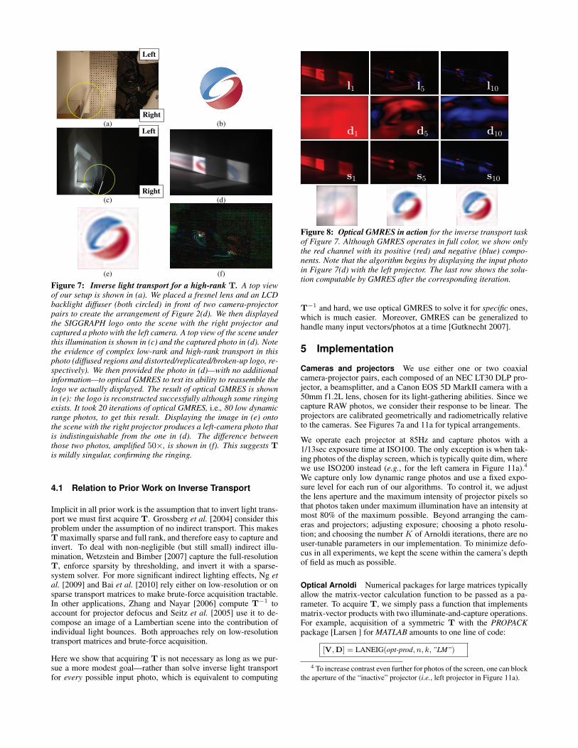
(e) (f)

Figure 7: Inverse light transport for a high-rank T. A top viewof our setup is shown in (a). We placed a fresnel lens and an LCDbacklight diffuser (both circled) in front of two camera-projectorpairs to create the arrangement of Figure 2(d). We then displayedthe SIGGRAPH logo onto the scene with the right projector andcaptured a photo with the left camera. A top view of the scene underthis illumination is shown in (c) and the captured photo in (d). Notethe evidence of complex low-rank and high-rank transport in thisphoto (diffused regions and distorted/replicated/broken-up logo, re-spectively). We then provided the photo in (d)—with no additionalinformation—to optical GMRES to test its ability to reassemble thelogo we actually displayed. The result of optical GMRES is shownin (e): the logo is reconstructed successfully although some ringingexists. It took 20 iterations of optical GMRES, i.e., 80 low dynamicrange photos, to get this result. Displaying the image in (e) ontothe scene with the right projector produces a left-camera photo thatis indistinguishable from the one in (d). The difference betweenthose two photos, amplified 50×, is shown in (f). This suggests Tis mildly singular, confirming the ringing.

4.1 Relation to Prior Work on Inverse Transport

Implicit in all prior work is the assumption that to invert light trans-port we must first acquire T. Grossberg et al. [2004] consider thisproblem under the assumption of no indirect transport. This makesT maximally sparse and full rank, and therefore easy to capture andinvert. To deal with non-negligible (but still small) indirect illu-mination, Wetzstein and Bimber [2007] capture the full-resolutionT, enforce sparsity by thresholding, and invert it with a sparse-system solver. For more significant indirect lighting effects, Ng etal. [2009] and Bai et al. [2010] rely either on low-resolution or onsparse transport matrices to make brute-force acquisition tractable.In other applications, Zhang and Nayar [2006] compute T−1 toaccount for projector defocus and Seitz et al. [2005] use it to de-compose an image of a Lambertian scene into the contribution ofindividual light bounces. Both approaches rely on low-resolutiontransport matrices and brute-force acquisition.

Here we show that acquiring T is not necessary as long as we pur-sue a more modest goal—rather than solve inverse light transportfor every possible input photo, which is equivalent to computing

l1 l5 l10

d1 d5 d10

s1 s5 s10

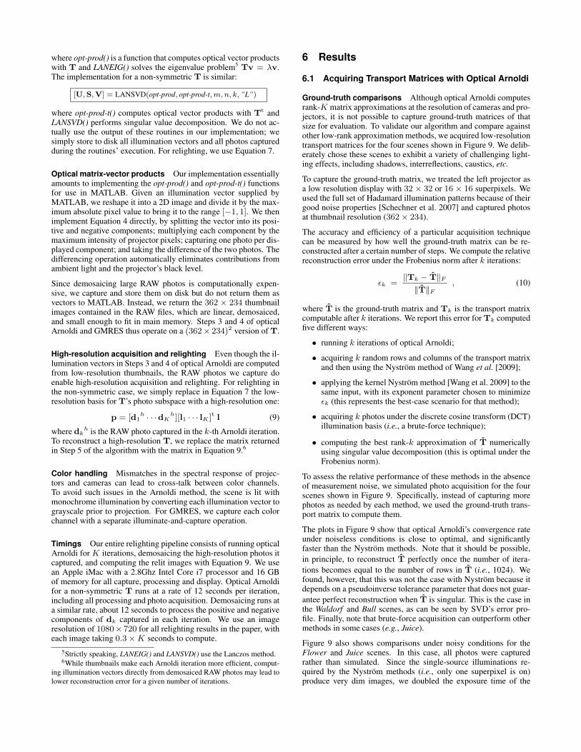
Figure 8: Optical GMRES in action for the inverse transport taskof Figure 7. Although GMRES operates in full color, we show onlythe red channel with its positive (red) and negative (blue) compo-nents. Note that the algorithm begins by displaying the input photoin Figure 7(d) with the left projector. The last row shows the solu-tion computable by GMRES after the corresponding iteration.

T−1 and hard, we use optical GMRES to solve it for specific ones,which is much easier. Moreover, GMRES can be generalized tohandle many input vectors/photos at a time [Gutknecht 2007].

5 Implementation

Cameras and projectors We use either one or two coaxialcamera-projector pairs, each composed of an NEC LT30 DLP pro-jector, a beamsplitter, and a Canon EOS 5D MarkII camera with a50mm f1.2L lens, chosen for its light-gathering abilities. Since wecapture RAW photos, we consider their response to be linear. Theprojectors are calibrated geometrically and radiometrically relativeto the cameras. See Figures 7a and 11a for typical arrangements.

We operate each projector at 85Hz and capture photos with a1/13sec exposure time at ISO100. The only exception is when tak-ing photos of the display screen, which is typically quite dim, wherewe use ISO200 instead (e.g., for the left camera in Figure 11a).4

We capture only low dynamic range photos and use a fixed expo-sure level for each run of our algorithms. To control it, we adjustthe lens aperture and the maximum intensity of projector pixels sothat photos taken under maximum illumination have an intensity atmost 80% of the maximum possible. Beyond arranging the cam-eras and projectors; adjusting exposure; choosing a photo resolu-tion; and choosing the number K of Arnoldi iterations, there are nouser-tunable parameters in our implementation. To minimize defo-cus in all experiments, we kept the scene within the camera’s depthof field as much as possible.

Optical Arnoldi Numerical packages for large matrices typicallyallow the matrix-vector calculation function to be passed as a pa-rameter. To acquire T, we simply pass a function that implementsmatrix-vector products with two illuminate-and-capture operations.For example, acquisition of a symmetric T with the PROPACKpackage [Larsen ] for MATLAB amounts to one line of code:

[V,D] = LANEIG(opt-prod, n, k, ”LM”)

4 To increase contrast even further for photos of the screen, one can block

the aperture of the “inactive” projector (i.e., left projector in Figure 11a).

where opt-prod() is a function that computes optical vector productswith T and LANEIG() solves the eigenvalue problem5 Tv = λv.The implementation for a non-symmetric T is similar:

[U,S,V] = LANSVD(opt-prod, opt-prod-t,m, n, k, ”L”)

where opt-prod-t() computes optical vector products with Tt andLANSVD() performs singular value decomposition. We do not ac-tually use the output of these routines in our implementation; wesimply store to disk all illumination vectors and all photos capturedduring the routines’ execution. For relighting, we use Equation 7.

Optical matrix-vector products Our implementation essentiallyamounts to implementing the opt-prod() and opt-prod-t() functionsfor use in MATLAB. Given an illumination vector supplied byMATLAB, we reshape it into a 2D image and divide it by the max-imum absolute pixel value to bring it to the range [−1, 1]. We thenimplement Equation 4 directly, by splitting the vector into its posi-tive and negative components; multiplying each component by themaximum intensity of projector pixels; capturing one photo per dis-played component; and taking the difference of the two photos. Thedifferencing operation automatically eliminates contributions fromambient light and the projector’s black level.

Since demosaicing large RAW photos is computationally expen-sive, we capture and store them on disk but do not return them asvectors to MATLAB. Instead, we return the 362 × 234 thumbnailimages contained in the RAW files, which are linear, demosaiced,and small enough to fit in main memory. Steps 3 and 4 of opticalArnoldi and GMRES thus operate on a (362× 234)2 version of T.

High-resolution acquisition and relighting Even though the il-lumination vectors in Steps 3 and 4 of optical Arnoldi are computedfrom low-resolution thumbnails, the RAW photos we capture doenable high-resolution acquisition and relighting. For relighting inthe non-symmetric case, we simply replace in Equation 7 the low-resolution basis for T’s photo subspace with a high-resolution one:

p = [d1h · · ·dK

h][l1 · · · lK ]t l (9)

where dkh is the RAW photo captured in the k-th Arnoldi iteration.

To reconstruct a high-resolution T, we replace the matrix returnedin Step 5 of the algorithm with the matrix in Equation 9.6

Color handling Mismatches in the spectral response of projec-tors and cameras can lead to cross-talk between color channels.To avoid such issues in the Arnoldi method, the scene is lit withmonochrome illumination by converting each illumination vector tograyscale prior to projection. For GMRES, we capture each colorchannel with a separate illuminate-and-capture operation.

Timings Our entire relighting pipeline consists of running opticalArnoldi for K iterations, demosaicing the high-resolution photos itcaptured, and computing the relit images with Equation 9. We usean Apple iMac with a 2.8Ghz Intel Core i7 processor and 16 GBof memory for all capture, processing and display. Optical Arnoldifor a non-symmetric T runs at a rate of 12 seconds per iteration,including all processing and photo acquisition. Demosaicing runs ata similar rate, about 12 seconds to process the positive and negativecomponents of dk captured in each iteration. We use an imageresolution of 1080× 720 for all relighting results in the paper, witheach image taking 0.3×K seconds to compute.

5Strictly speaking, LANEIG() and LANSVD() use the Lanczos method.6While thumbnails make each Arnoldi iteration more efficient, comput-

ing illumination vectors directly from demosaiced RAW photos may lead to

lower reconstruction error for a given number of iterations.

6 Results

6.1 Acquiring Transport Matrices with Optical Arnoldi

Ground-truth comparisons Although optical Arnoldi computesrank-K matrix approximations at the resolution of cameras and pro-jectors, it is not possible to capture ground-truth matrices of thatsize for evaluation. To validate our algorithm and compare againstother low-rank approximation methods, we acquired low-resolutiontransport matrices for the four scenes shown in Figure 9. We delib-erately chose these scenes to exhibit a variety of challenging light-ing effects, including shadows, interreflections, caustics, etc.

To capture the ground-truth matrix, we treated the left projector asa low resolution display with 32 × 32 or 16 × 16 superpixels. Weused the full set of Hadamard illumination patterns because of theirgood noise properties [Schechner et al. 2007] and captured photosat thumbnail resolution (362× 234).

The accuracy and efficiency of a particular acquisition techniquecan be measured by how well the ground-truth matrix can be re-constructed after a certain number of steps. We compute the relativereconstruction error under the Frobenius norm after k iterations:

ǫk =‖Tk − T‖F

‖T‖F, (10)

where T is the ground-truth matrix and Tk is the transport matrixcomputable after k iterations. We report this error for Tk computedfive different ways:

• running k iterations of optical Arnoldi;

• acquiring k random rows and columns of the transport matrixand then using the Nystrom method of Wang et al. [2009];

• applying the kernel Nystrom method [Wang et al. 2009] to thesame input, with its exponent parameter chosen to minimizeǫk (this represents the best-case scenario for that method);

• acquiring k photos under the discrete cosine transform (DCT)illumination basis (i.e., a brute-force technique);

• computing the best rank-k approximation of T numericallyusing singular value decomposition (this is optimal under theFrobenius norm).

To assess the relative performance of these methods in the absenceof measurement noise, we simulated photo acquisition for the fourscenes shown in Figure 9. Specifically, instead of capturing morephotos as needed by each method, we used the ground-truth trans-port matrix to compute them.

The plots in Figure 9 show that optical Arnoldi’s convergence rateunder noiseless conditions is close to optimal, and significantlyfaster than the Nystrom methods. Note that it should be possible,

in principle, to reconstruct T perfectly once the number of itera-

tions becomes equal to the number of rows in T (i.e., 1024). Wefound, however, that this was not the case with Nystrom because itdepends on a pseudoinverse tolerance parameter that does not guar-

antee perfect reconstruction when T is singular. This is the case inthe Waldorf and Bull scenes, as can be seen by SVD’s error pro-file. Finally, note that brute-force acquisition can outperform othermethods in some cases (e.g., Juice).

Figure 9 also shows comparisons under noisy conditions for theFlower and Juice scenes. In this case, all photos were capturedrather than simulated. Since the single-source illuminations re-quired by the Nystrom methods (i.e., only one superpixel is on)produce very dim images, we doubled the exposure time of the

Wa

ldo

rfreplacements

0.5

102400

Nyström

kernel Nyström

brute-force (DCT)

optical Arnoldi

optimal (SVD)

# iterations

rela

tive

erro

r

Bu

ll

0.5

102400 # iterations

rela

tive

erro

r

Flo

wer

0.5

25600

Noisy

Noiseless

# iterations

rela

tive

erro

r

Ora

ng

eju

ice

0.5

25600 # iterations

rela

tive

erro

r

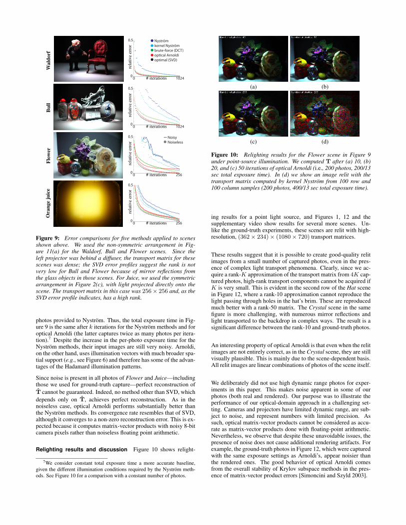
Figure 9: Error comparisons for five methods applied to scenesshown above. We used the non-symmetric arrangement in Fig-ure 11(a) for the Waldorf, Bull and Flower scenes. Since theleft projector was behind a diffuser, the transport matrix for thesescenes was dense; the SVD error profiles suggest the rank is notvery low for Bull and Flower because of mirror reflections fromthe glass objects in those scenes. For Juice, we used the symmetricarrangement in Figure 2(c), with light projected directly onto thescene. The transport matrix in this case was 256× 256 and, as theSVD error profile indicates, has a high rank.

photos provided to Nystrom. Thus, the total exposure time in Fig-ure 9 is the same after k iterations for the Nystrom methods and foroptical Arnoldi (the latter captures twice as many photos per itera-tion).7 Despite the increase in the per-photo exposure time for theNystrom methods, their input images are still very noisy. Arnoldi,on the other hand, uses illumination vectors with much broader spa-tial support (e.g., see Figure 6) and therefore has some of the advan-tages of the Hadamard illumination patterns.

Since noise is present in all photos of Flower and Juice—includingthose we used for ground-truth capture—perfect reconstruction of

T cannot be guaranteed. Indeed, no method other than SVD, which

depends only on T, achieves perfect reconstruction. As in thenoiseless case, optical Arnoldi performs substantially better thanthe Nystrom methods. Its convergence rate resembles that of SVD,although it converges to a non-zero reconstruction error. This is ex-pected because it computes matrix-vector products with noisy 8-bitcamera pixels rather than noiseless floating point arithmetic.

Relighting results and discussion Figure 10 shows relight-

7We consider constant total exposure time a more accurate baseline,

given the different illumination conditions required by the Nystrom meth-

ods. See Figure 10 for a comparison with a constant number of photos.

(a) (b)

(c) (d)

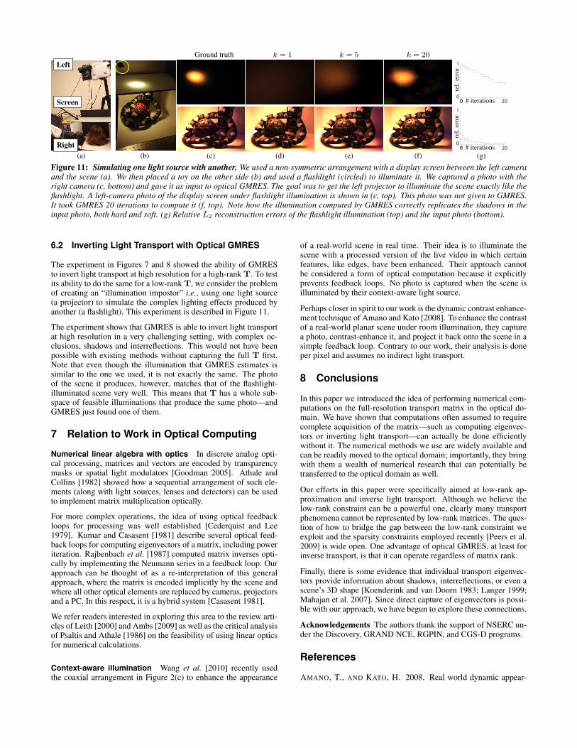
Figure 10: Relighting results for the Flower scene in Figure 9under point-source illumination. We computed T after (a) 10, (b)20, and (c) 50 iterations of optical Arnoldi (i.e., 200 photos, 200/13sec total exposure time). In (d) we show an image relit with thetransport matrix computed by kernel Nystrom from 100 row and100 column samples (200 photos, 400/13 sec total exposure time).

ing results for a point light source, and Figures 1, 12 and thesupplementary video show results for several more scenes. Un-like the ground-truth experiments, these scenes are relit with high-resolution, (362× 234)× (1080× 720) transport matrices.

These results suggest that it is possible to create good-quality relitimages from a small number of captured photos, even in the pres-ence of complex light transport phenomena. Clearly, since we ac-quire a rank-K approximation of the transport matrix from 4K cap-tured photos, high-rank transport components cannot be acquired ifK is very small. This is evident in the second row of the Hat scenein Figure 12, where a rank-10 approximation cannot reproduce thelight passing through holes in the hat’s brim. These are reproducedmuch better with a rank-50 matrix. The Crystal scene in the samefigure is more challenging, with numerous mirror reflections andlight transported to the backdrop in complex ways. The result is asignificant difference between the rank-10 and ground-truth photos.

An interesting property of optical Arnoldi is that even when the relitimages are not entirely correct, as in the Crystal scene, they are stillvisually plausible. This is mainly due to the scene-dependent basis.All relit images are linear combinations of photos of the scene itself.

We deliberately did not use high dynamic range photos for exper-iments in this paper. This makes noise apparent in some of ourphotos (both real and rendered). Our purpose was to illustrate theperformance of our optical-domain approach in a challenging set-ting. Cameras and projectors have limited dynamic range, are sub-ject to noise, and represent numbers with limited precision. Assuch, optical matrix-vector products cannot be considered as accu-rate as matrix-vector products done with floating-point arithmetic.Nevertheless, we observe that despite these unavoidable issues, thepresence of noise does not cause additional rendering artifacts. Forexample, the ground-truth photos in Figure 12, which were capturedwith the same exposure settings as Arnoldi’s, appear noisier thanthe rendered ones. The good behavior of optical Arnoldi comesfrom the overall stability of Krylov subspace methods in the pres-ence of matrix-vector product errors [Simoncini and Szyld 2003].

Ground truth k = 1 k = 5 k = 20

Left

Right

Screen

1

00 200 # iterations

rel.

erro

r

1

00

200 # iterations

rel.

erro

r

(a) (b) (c) (d) (e) (f) (g)

Figure 11: Simulating one light source with another. We used a non-symmetric arrangement with a display screen between the left cameraand the scene (a). We then placed a toy on the other side (b) and used a flashlight (circled) to illuminate it. We captured a photo with theright camera (c, bottom) and gave it as input to optical GMRES. The goal was to get the left projector to illuminate the scene exactly like theflashlight. A left-camera photo of the display screen under flashlight illumination is shown in (c, top). This photo was not given to GMRES.It took GMRES 20 iterations to compute it (f, top). Note how the illumination computed by GMRES correctly replicates the shadows in theinput photo, both hard and soft. (g) Relative L2 reconstruction errors of the flashlight illumination (top) and the input photo (bottom).

6.2 Inverting Light Transport with Optical GMRES

The experiment in Figures 7 and 8 showed the ability of GMRESto invert light transport at high resolution for a high-rank T. To testits ability to do the same for a low-rank T, we consider the problemof creating an “illumination impostor” i.e., using one light source(a projector) to simulate the complex lighting effects produced byanother (a flashlight). This experiment is described in Figure 11.

The experiment shows that GMRES is able to invert light transportat high resolution in a very challenging setting, with complex oc-clusions, shadows and interreflections. This would not have beenpossible with existing methods without capturing the full T first.Note that even though the illumination that GMRES estimates issimilar to the one we used, it is not exactly the same. The photoof the scene it produces, however, matches that of the flashlight-illuminated scene very well. This means that T has a whole sub-space of feasible illuminations that produce the same photo—andGMRES just found one of them.

7 Relation to Work in Optical Computing

Numerical linear algebra with optics In discrete analog opti-cal processing, matrices and vectors are encoded by transparencymasks or spatial light modulators [Goodman 2005]. Athale andCollins [1982] showed how a sequential arrangement of such ele-ments (along with light sources, lenses and detectors) can be usedto implement matrix multiplication optically.

For more complex operations, the idea of using optical feedbackloops for processing was well established [Cederquist and Lee1979]. Kumar and Casasent [1981] describe several optical feed-back loops for computing eigenvectors of a matrix, including poweriteration. Rajbenbach et al. [1987] computed matrix inverses opti-cally by implementing the Neumann series in a feedback loop. Ourapproach can be thought of as a re-interpretation of this generalapproach, where the matrix is encoded implicitly by the scene andwhere all other optical elements are replaced by cameras, projectorsand a PC. In this respect, it is a hybrid system [Casasent 1981].

We refer readers interested in exploring this area to the review arti-cles of Leith [2000] and Ambs [2009] as well as the critical analysisof Psaltis and Athale [1986] on the feasibility of using linear opticsfor numerical calculations.

Context-aware illumination Wang et al. [2010] recently usedthe coaxial arrangement in Figure 2(c) to enhance the appearance

of a real-world scene in real time. Their idea is to illuminate thescene with a processed version of the live video in which certainfeatures, like edges, have been enhanced. Their approach cannotbe considered a form of optical computation because it explicitlyprevents feedback loops. No photo is captured when the scene isilluminated by their context-aware light source.

Perhaps closer in spirit to our work is the dynamic contrast enhance-ment technique of Amano and Kato [2008]. To enhance the contrastof a real-world planar scene under room illumination, they capturea photo, contrast-enhance it, and project it back onto the scene in asimple feedback loop. Contrary to our work, their analysis is doneper pixel and assumes no indirect light transport.

8 Conclusions

In this paper we introduced the idea of performing numerical com-putations on the full-resolution transport matrix in the optical do-main. We have shown that computations often assumed to requirecomplete acquisition of the matrix—such as computing eigenvec-tors or inverting light transport—can actually be done efficientlywithout it. The numerical methods we use are widely available andcan be readily moved to the optical domain; importantly, they bringwith them a wealth of numerical research that can potentially betransferred to the optical domain as well.

Our efforts in this paper were specifically aimed at low-rank ap-proximation and inverse light transport. Although we believe thelow-rank constraint can be a powerful one, clearly many transportphenomena cannot be represented by low-rank matrices. The ques-tion of how to bridge the gap between the low-rank constraint weexploit and the sparsity constraints employed recently [Peers et al.2009] is wide open. One advantage of optical GMRES, at least forinverse transport, is that it can operate regardless of matrix rank.

Finally, there is some evidence that individual transport eigenvec-tors provide information about shadows, interreflections, or even ascene’s 3D shape [Koenderink and van Doorn 1983; Langer 1999;Mahajan et al. 2007]. Since direct capture of eigenvectors is possi-ble with our approach, we have begun to explore these connections.

Acknowledgements The authors thank the support of NSERC un-der the Discovery, GRAND NCE, RGPIN, and CGS-D programs.

References

AMANO, T., AND KATO, H. 2008. Real world dynamic appear-

ance enhancement with procam feedback. Proc. IEEE PRO-CAMS.

AMBS, P. 2009. A short history of optical computing: rise, decline,and evolution. Proc. SPIE 7388.

ATHALE, R. A., AND COLLINS, W. C., 1982. Optical matrix-matrix multiplier based on outer product decomposition.

BAI, J., CHANDRAKER, M., NG, T.-T., AND RAMAMOORTHI,R. 2010. A dual theory of inverse and forward light transport.Proc. ECCV .

BASRI, R., AND JACOBS, D. 2003. Lambertian reflectance andlinear subspaces. IEEE T-PAMI 25, 2, 218–233.

CASASENT, D. 1981. Hybrid processors. Optical InformationProcessing Fundamentals, 181–233.

CEDERQUIST, J., AND LEE, S. 1979. The use of feedback inoptical information processing. Applied Physics A: MaterialsScience & Processing.

DEBEVEC, P., HAWKINS, T., TCHOU, C., DUIKER, H.-P.,SAROKIN, W., AND SAGAR, M. 2000. Acquiring the re-flectance field of a human face. Proc. SIGGRAPH.

FUCHS, M., BLANZ, V., LENSCH, H., AND SEIDEL, H.-P. 2007.Adaptive sampling of reflectance fields. ACM TOG 26, 2 (Jun).

GARG, G., TALVALA, E., LEVOY, M., AND LENSCH, H.2006. Symmetric photography: Exploiting data-sparseness inreflectance fields. Proc. Eurographics Symp. Rendering.

GOODMAN, J. W. 2005. Introduction to fourier optics, 3rd edition.Roberts & Company Publishers.

GREENBAUM, A., AND TREFETHEN, L. N. 1994. Gmres/cr andarnoldi/lanczos as matrix approximation problems. SIAM J. Sci.Comput. 15, 2, 359–368.

GROSSBERG, M., PERI, H., NAYAR, S., AND BELHUMEUR, P.2004. Making one object look like another: controlling appear-ance using a projector-camera system. Proc. CVPR, 452–459.

GUILFOYLE, P., AND STONE, R. 1991. Digital optical computerii. Proc. SPIE 1563, 214–222.

GUTKNECHT, M. H. 2007. Block krylov space methods for lin-ear systems with multiple right-hand sides: an introduction. InModern Mathematical Models, Methods and Algorithms for RealWorld Systems. 420–447.

KOENDERINK, J. J., AND VAN DOORN, A. J. 1983. Geometri-cal modes as a general method to treat diffuse interreflections inradiometry. J. Opt. Soc. Am 73, 6, 843–850.

KUMAR, B. V. K. V., AND CASASENT, D. 1981. Eigenvectordetermination by iterative optical methods. Applied Optics 20,21, 3707–3710.

LANGER, M. 1999. When shadows become interreflections. Int. J.Computer Vision 34, 2, 193–204.

LARSEN, R. M. http://soi.stanford.edu/ rmunk/propack/.

LEITH, E. 2000. The evolution of information optics. IEEE J.Select Topics in Quantum Electronics 6, 6, 1297–1304.

LIESEN, J., AND TICHY, P. 2004. Convergence analysis of krylovsubspace methods. GAMM Mitt. Ges. Angew. Math. Mech. 27,2, 153–173 (2005).

MAHAJAN, D., SHLIZERMAN, I., RAMAMOORTHI, R., AND

BELHUMEUR, P. 2007. A theory of locally low dimensionallight transport. Proc. SIGGRAPH.

MATUSIK, W., PFISTER, H., ZIEGLER, R., AND NGAN, A. 2002.Acquisition and rendering of transparent and refractive objects.Proc. Eurographics Symp. on Rendering.

NG, R., RAMAMOORTHI, R., AND HANRAHAN, P. 2003. All-frequency shadows using non-linear wavelet lighting approxima-tion. Proc. SIGGRAPH.

NG, T., PAHWA, R., BAI, J., QUEK, T., AND TAN, K. 2009.Radiometric compensation using stratified inverses. Proc. ICCV .

PEERS, P., AND DUTRE, P. 2003. Wavelet environment matting.Proc. Eurographics Symp. on Rendering.

PEERS, P., AND DUTRE, P. 2005. Inferring reflectance functionsfrom wavelet noise. Proc. Eurographics Symp. Rendering.

PEERS, P., MAHAJAN, D., LAMOND, B., GHOSH, A., MATUSIK,W., RAMAMOORTHI, R., AND DEBEVEC, P. 2009. Compres-sive light transport sensing. ACM TOG 28, 1.

PSALTIS, D., AND ATHALE, R. A. 1986. High accuracy computa-tion with linear analog optical systems: a cricitcal study. AppliedOptics 25, 18, 3071–3077.

RAJBENBACH, H., FAINMAN, Y., AND LEE, S. H. 1987. Opticalimplementation of an interative algorithm for matrix-inversion.Applied Optics 26, 6, 1024–1031.

SAAD, Y. 2003. Iterative methods for sparse linear systems.

SALVI, J., PAGES, J., AND BATLLE, J. 2004. Pattern codificationstrategies in structured light systems. Pattern Recogn 37, 4, 827–849.

SCHECHNER, Y., NAYAR, S., AND BELHUMEUR, P. 2007. Mul-tiplexing for optimal lighting. IEEE T-PAMI 29, 8, 1339–1354.

SEITZ, S., MATSUSHITA, Y., AND KUTULAKOS, K. 2005. Atheory of inverse light transport. Proc. ICCV , 1440—1447.

SEN, P., AND DARABI, S. 2009. Compressive dual photography.Proc. Eurographics.

SEN, P., CHEN, B., GARG, G., MARSCHNER, S., HOROWITZ,M., LEVOY, M., AND LENSCH, H. 2005. Dual photography.Proc. SIGGRAPH.

SIMON, H. D., AND ZHA, H. 2000. Low-rank matrix approxi-mation using the lanczos bidiagonalization process with applica-tions. SIAM J. Sci. Comput. 21, 6, 2257–2274.

SIMONCINI, V., AND SZYLD, D. B. 2003. Theory of inexactkrylov subspace methods and applications to scientific comput-ing. SIAM J. Sci. Comput. 25, 2, 454–477.

TREFETHEN, L. N., AND BAU, I. 1997. Numerical linear algebra.SIAM, xii+361.

WANG, J., DONG, Y., TONG, X., LIN, Z., AND GUO, B. 2009.Kernel nystrom method for light transport. Proc. SIGGRAPH.

WANG, O., FUCHS, M., FUCHS, C., DAVIS, J., SEIDEL, H.-P.,AND LENSCH, H. P. A. 2010. A context-aware light source.Proc. ICCP.

WETZSTEIN, G., AND BIMBER, O. 2007. Radiometric compensa-tion through inverse light transport. Pacific Graphics, 391–399.

ZHANG, L., AND NAYAR, S. 2006. Projection defocus analysisfor scene capture and image display. Proc. SIGGRAPH.

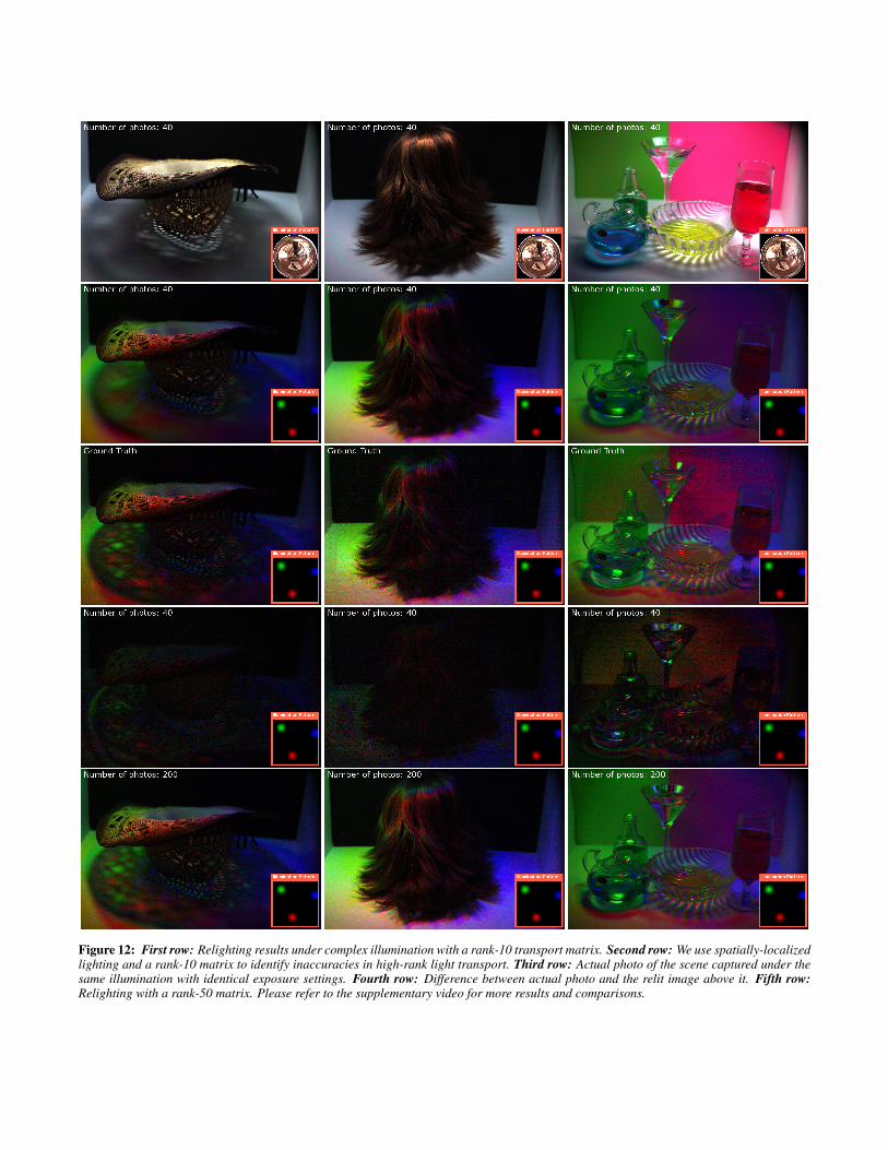
Figure 12: First row: Relighting results under complex illumination with a rank-10 transport matrix. Second row: We use spatially-localizedlighting and a rank-10 matrix to identify inaccuracies in high-rank light transport. Third row: Actual photo of the scene captured under thesame illumination with identical exposure settings. Fourth row: Difference between actual photo and the relit image above it. Fifth row:Relighting with a rank-50 matrix. Please refer to the supplementary video for more results and comparisons.