Embed Size (px)
Citation preview
Class. Quantum Grav. 17 (2000) 2691–2718. Printed in the UK PII: S0264-9381(00)08663-9
Optical reference geometry of Kerr–Newman spacetimes
Z Stuchlık, S Hledık and J JuranDepartment of Physics, Faculty of Philosophy and Science, Silesian University at Opava,Bezrucovo nam. 13, 746 01 Opava, Czech Republic
E-mail: [email protected], [email protected] [email protected]
Received 13 October 1999, in final form 16 March 2000
Abstract. Properties of the optical reference geometry related to Kerr–Newman black-hole andnaked-singularity spacetimes are illustrated using embedding diagrams of their equatorial plane. Itis shown that among all inertial forces defined within the framework of the optical geometry, justthe centrifugal force plays a fundamental role in connection with the embedding diagrams becauseit changes sign at the turning points of the diagrams. The embedding diagrams do not cover thestationary part of the Kerr–Newman spacetimes completely. Hence, the limits of embeddabilityare given, and it is established which of the photon circular orbits hosted by the Kerr–Newmanspacetimes appear in the embeddable regions. Some typical embedding diagrams are constructed,and the Kerr–Newman backgrounds are classified according to the number of embeddable regionsof the optical geometry as well as the number of their turning points. It is shown that embeddingdiagrams are closely related to the notion of the radius of gyration which is useful for analysing afluid rotating in strong gravitational fields.
(Some figures in this article are in colour only in the electronic version; see www.iop.org)
PACS numbers: 0470B, 0470, 0425
1. Introduction
The optical reference geometry related to stationary spacetimes enables one to introduce theconcept of inertial forces within the framework of general relativity in a natural way [1, 2]. Ofcourse, in accord with the spirit of general relativity, alternative approaches to the concept ofinertial forces are possible (see, e.g., [3, 4]); however, here we shall follow the approach ofAbramowicz and his co-workers [5], providing a description of relativistic dynamics in accordwith Newtonian intuition.
The optical geometry results from an appropriate conformal (3 + 1) splitting, reflectingsome hidden properties of the spacetimes under consideration through its geodesic structure.The geodesics of the optical geometry related to static spacetimes coincide with trajectories oflight, thus being ‘optically straight’ [6, 7]. Moreover, the geodesics are ‘dynamically straight’,because test particles moving along them are kept by a velocity-independent force [8]; theyare also ‘inertially straight’, because gyroscopes carried along them do not precess along thedirection of motion [9].
Some properties of the optical geometry can be appropriately demonstrated by embeddingdiagrams of its representative sections [1, 10, 11]. Because we are familiar with Euclideanspace, usually two-dimensional sections of the optical space are embedded into the three-dimensional Euclidean space. (Of course, embeddings into other conveniently chosen spaces
0264-9381/00/142691+28$30.00 © 2000 IOP Publishing Ltd 2691
2692 Z Stuchlık et al
can also provide interesting information, however, we shall focus our attention on the moststraightforward Euclidean case.) In the Kerr–Newman backgrounds, the most representativesection is the equatorial plane, which is their symmetry plane. This plane is also of greatastrophysical importance, especially in connection to the theory of accretion discs [12].
In the spherically symmetric spacetimes (Schwarzschild [6], Reissner–Nordstrom [10]and Schwarzschild–de Sitter [13]), an interesting coincidence appears: the turning points ofthe central-plane embedding diagrams of the optical space and the photon circular orbits arelocated at the same radii, where, moreover, the centrifugal force, related to the optical space,vanishes and reverses sign.
However, in the rotating black-hole and naked-singularity backgrounds, the centrifugalforce does not vanish at the radii of photon circular orbits in the equatorial plane [14]. Of course,the same statement is true if these rotating backgrounds carry a non-zero electric charge. Itis, therefore, interesting to study how the inertial forces, defined within the framework of theoptical geometry, and the photon circular orbits are related to equatorial-plane embeddingdiagrams of the optical geometry of rotating, charged backgrounds. Such relations werediscussed in the case of non-charged, Kerr backgrounds in [15]. In this paper, we shallgeneralize the results to the more complex case of the Kerr–Newman backgrounds, in whicheven stable photon circular orbits can exist beside the unstable ones, contrary to the case ofKerr backgrounds [16].
In section 2, the optical reference geometry and the related inertial forces are definedrelative to the family of locally non-rotating observers in the Kerr–Newman spacetimes. Insection 3, stationary equatorial circular motion in the Kerr–Newman spacetimes is discussed,using the concept of the gravitational and inertial forces expressed in terms of a ‘Newtonian’velocity related to the optical geometry. It is shown that asymptotically the relativisticexpressions of the gravitational, Coriolis and centrifugal forces reduce to the well knownNewtonian formulae. In central parts, they enable an illumination of unusual properties ofthe Kerr–Newman spacetimes in terms of intuitively clear concepts. The properties of thecentrifugal force in the equatorial plane are closely related to the properties of the embeddingdiagrams of the optical-geometry equatorial plane. In section 4, the embedding formula isintroduced, the limits of Euclidean embeddability of the optical geometry are established,and the turning points of the embedding diagrams are determined; it is also shown thatthey occur just where the centrifugal force reverses sign. The locations of photon circularorbits in the equatorial plane are given, and it is established which of them are containedin the embeddable regions of the optical space. The Kerr–Newman spacetimes are classifiedaccording to the criterion of embeddability of regions containing photon circular orbits. Finally,typical embedding diagrams are constructed, and the Kerr–Newman spacetimes are classifiedaccording to the properties of the embedding diagrams (namely, the numbers of embeddableregions and turning points of the diagrams). In section 5, some concluding remarks arepresented.
2. Optical geometry and inertial forces
The notion of the optical reference geometry and related inertial forces are convenient forspacetimes with symmetries, especially for stationary (static) and axisymmetric (sphericallysymmetric) ones. However, they can be introduced for a general spacetime lacking anysymmetry [2].
Optical reference geometry of Kerr–Newman spacetimes 2693
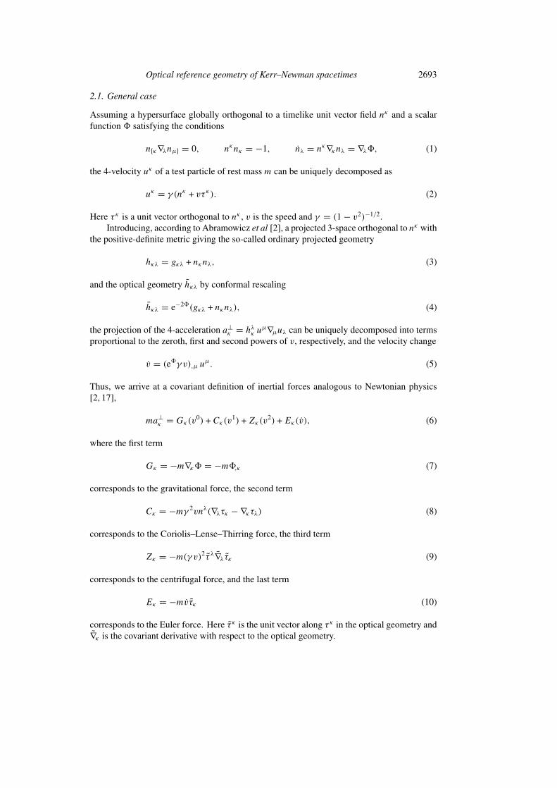
2.1. General case
Assuming a hypersurface globally orthogonal to a timelike unit vector field nκ and a scalarfunction � satisfying the conditions
n[κ∇λnµ] = 0, nκnκ = −1, nλ = nκ∇κnλ = ∇λ�, (1)
the 4-velocity uκ of a test particle of rest mass m can be uniquely decomposed as
uκ = γ (nκ + vτκ). (2)
Here τ κ is a unit vector orthogonal to nκ , v is the speed and γ = (1 − v2)−1/2.Introducing, according to Abramowicz et al [2], a projected 3-space orthogonal to nκ with
the positive-definite metric giving the so-called ordinary projected geometry
hκλ = gκλ + nκnλ, (3)
and the optical geometry hκλ by conformal rescaling
hκλ = e−2�(gκλ + nκnλ), (4)
the projection of the 4-acceleration a⊥κ = hλκ u
µ∇µuλ can be uniquely decomposed into termsproportional to the zeroth, first and second powers of v, respectively, and the velocity change
v = (e�γ v),µ uµ. (5)
Thus, we arrive at a covariant definition of inertial forces analogous to Newtonian physics[2, 17],
ma⊥κ = Gκ(v
0) + Cκ(v1) + Zκ(v
2) + Eκ(v), (6)
where the first term
Gκ = −m∇κ� = −m�,κ (7)
corresponds to the gravitational force, the second term
Cκ = −mγ 2vnλ(∇λτκ − ∇κτλ) (8)
corresponds to the Coriolis–Lense–Thirring force, the third term
Zκ = −m(γ v)2τ λ∇λτκ (9)
corresponds to the centrifugal force, and the last term
Eκ = −mvτκ (10)
corresponds to the Euler force. Here τ κ is the unit vector along τ κ in the optical geometry and∇κ is the covariant derivative with respect to the optical geometry.
2694 Z Stuchlık et al
2.2. Kerr–Newman case
Using a geometric system of units (c = G = 1), and denoting by M the mass, a the specificangular momentum, e the electric charge, then the line element of the Kerr–Newman spacetime,expressed in terms of standard Boyer–Lindquist coordinates, reads
ds2 = −(
1 − 2Mr − e2
�
)dt2 − 2a(2Mr − e2)
�sin2 θ dt dφ
+A sin2 θ
�dφ2 +
�
!dr2 +� dθ2, (11)
where
! = r2 − 2Mr + a2 + e2, (12)
� = r2 + a2 cos2 θ, (13)
A = (r2 + a2)2 −!a2 sin2 θ. (14)
For simplicity we put M = 1 in the following; equivalently, we use mass units of M . Ifa2 + e2 � 1, the metric (11) represents black-hole spacetimes. The loci of their horizons, r−(the inner one) and r+ (the outer one), determined by real roots of!(r; a, e) = 0, can be givenequivalently by the relation
a2 = a2h(r; e) = r(2 − r)− e2. (15)
The case a2 +e2 = 1 corresponds to extreme black holes. If a2 +e2 > 1, there are no horizons,and the metric (11) represents a naked-singularity spacetime. If e2 < 1, both the black-holeand naked-singularity spacetimes contain an ergosphere, where gtt < 0; particles and photonsin bound states with covariant energy E < 0 are possible there [18]. Naked-singularityspacetimes with e2 � 1 have no ergosphere.
The Kerr–Newman spacetimes, being stationary and axially symmetric, admit twocommuting Killing vector fields; the vector field ηκ is (at least asymptotically) timelike, havingopen trajectories, the vector field ξκ is spacelike, having closed trajectories. Now, the vectorfield nκ relevant for constructions of the ordinary projected geometry and the optical referencegeometry can be given by using these Killing vector fields [5], and corresponds to the family oflocally non-rotating frames (LNRF) or zero angular momentum observers (ZAMO) introducedby Bardeen [12]; namely,
nκ = e�(ηκ +&LNRFξκ), &LNRF = −ξληλ/ηµηµ,
� = − 12 ln
(−ηληλ − 2&LNRFξληλ −&2
LNRFξλξλ
).
(16)
The LNRF vector field nκ can be used for the definition of inertial forces introduced above.Assuming a circular motion with angular velocity & = dφ/dt as measured by the stationaryobservers at infinity, the 4-velocity is given by
uκ = A(ηκ +&ξκ), A = (−ηληλ − 2&ξληλ −&2ξλξλ)−1/2 ; (17)
now τ κ is directed along the rotational Killing vector ξκ . The gravitational (7), Coriolis–Lense–Thirring (8), and centrifugal (9) forces can be written down as
Gκ = −m�,κ = −1
2m∂κ
[ln
(g2tφ − gttgφφ
gφφ
)], (18)
Optical reference geometry of Kerr–Newman spacetimes 2695
Cκ = mA2&−&LNRF
ξλξλ
[(ξλξλ)(η
µξµ),κ − (ηµξµ)(ξλξλ),κ
]= mA2(&−&LNRF)
√gφφ
[∂κ
(gtφg
−1/2φφ
)+&LNRF ∂κ
√gφφ
], (19)
Zκ = 12mA
2 (&−&LNRF)2
ιλιλ
[(ιλιλ)(ξ
µξµ),κ − (ξµξµ)(ιλιλ),κ
]
= − 12mA
2(&−&LNRF)2gφφ ∂κ
[ln
(g2φφ
g2tφ − gttgφφ
)], (20)
respectively; we denote ικ = e−�nκ . The Euler force will appear for& �= constant only, beingdetermined by & = uλ∇λ& (see [5]). The electromagnetic forces acting in charged spacetimeswere defined within the framework of the optical geometry in [17, 19]. However, here we shallconcentrate on the inertial forces acting on the motion in the equatorial plane (θ = π/2), andtheir relation to the embedding diagram of the equatorial plane of the optical geometry.
Clearly, by definition, the gravitational force is independent of the velocity of the orbitingparticle. On the other hand, both the Coriolis–Lense–Thirring and the centrifugal force vanish(at any r) if & = &LNRF, i.e. if the orbiting particle is stationary at the LNRF located at theradius of the circular orbit. This fact clearly illustrates that the LNRF are properly chosen forthe definition of the optical geometry and inertial forces in accord with Newtonian intuition.Moreover, both the forces vanish at some radii independently of&. In the case of the centrifugalforce, this property will be imprinted into the structure of the embedding diagrams.
3. Stationary equatorial circular motion in the Kerr–Newman spacetimes
For the stationary circular motion, & = 0. It is convenient to express the inertial forces interms of the ‘Newtonian’ velocity
v = γ v. (21)
The velocity v takes values from −∞ to ∞, while v from −1 to 1. In the stationary and axiallysymmetric spacetimes, there is
v = &R, (22)
where
& = &−&LNRF, R = re�, r = (ξκξκ)1/2. (23)
R is the so-called radius of gyration, because R2 = +/&, where + = L/E is the specific angularmomentum, L = Uκξκ is the angular momentum andE = −Uκηκ = γ e� is the energy [5, 7].It plays a very important role in the theory of rotational effects in strong gravitational fields.The direction of increase of the radius of gyration gives a preferred determination of thelocal outward direction relevant for the dynamical effects of rotation. This direction becomesmisaligned with the ‘global’ outward direction in strong fields [7]. The condition R = constantdefines the von Zeipel cylinders in stationary spacetimes, which are related to the equipotentialsurfaces of equilibrium configurations of a perfect fluid [20].
It is convenient to introduce the gravitational acceleration, and the velocity-independentparts of the Coriolis and centrifugal accelerations in the direction eκ by the relations [5]
G(r) = eκ∇κ�, C(r) = eκR∇κ&LNRF, Z(r) = eκR−1∇κ R. (24)
2696 Z Stuchlık et al
The acceleration necessary to keep a particle in stationary motion with a velocity v along acircle r = constant in the equatorial plane can then be expressed in a very simple form,
a(v, r) = −G(r)− v2Z(r) + (1 + v2)1/2vC(r) (25)
that enables an effective discussion of the properties of both accelerated and geodesic motion.(Of course, only the positive root of the last term on the right-hand side of equation (25) hasphysical meaning.)
For the stationary circular motion in the equatorial plane of the Kerr–Newman spacetimesall three parts of the acceleration have only radial components. We obtain
G(r) = − r4(r − e2) + a2[2r(r − 2)(r − e2)− e4] + a4(r − e2)
r![(r2 + a2)2 − a2!], (26)
C(r) = −2a[r(3r2 + a2)− e2(2r + a2)]
r√! [(r2 + a2)2 − a2!]
, (27)
Z(r) = {r![(r2 + a2)2 − a2!]
}−1 {r4(r2 − 3r + 2e2)
+ a2[r2(r2 − 3r + 6) + e2r(3r − 7) + 2e4] − 2a4(r − e2)}. (28)
These definitions of the gravitational and inertial forces have really a Newtonian character,since the gravitational force G = −mG(r) is velocity independent, C = m(1 + v2)1/2vC(r)depends on v, and the centrifugal force Z = −mv2Z(r) depends on v2. Moreover, theasymptotic behaviour of these forces is consistent with ‘Newtonian’ intuition:
G(r → ∞) ∼ − 1
r2, C(r → ∞) ∼ − a
r3, Z(r → ∞) ∼ 1
r. (29)
It follows immediately from equation (25) that the photon circular geodesic motion(v2 → ∞) is determined by the conditions
Z(r)− C(r) = 0, corotating orbits, (30)
Z(r) + C(r) = 0, counter-rotating orbits. (31)
For ultrarelativistic particles (v � 1, v −1), we obtain an asymptotic relation
a(v, r) ≈ −G(r)± 12C(r)− v2[Z(r)∓ C(r)]. (32)
The upper signs correspond to the corotating motion (v > 0) and the lower signs to the counter-rotating (v < 0) motion. The ultrarelativistic particles moving on the radius of the corotating(counter-rotating) photon circular geodesic are kept by the acceleration
a(r) = −G(r)± 12C(r), (33)
which is independent of velocity, with accuracy O(v−2). In static spacetimes C(r) = 0, and atthe radius of the photon circular orbit the acceleration of particles is
a(r) = −G(r), (34)
and is independent of v exactly. (The relation (34) is not limited to the case of ultrarelativisticorbits, because Z(r) = 0 at the radius of the photon circular geodesics in static spacetimes.)
The velocity of particles moving along the circular geodesics is determined by the relation
v2± =
12C2 − ZG ∓ 1
2C(C2 − 4ZG + 4G2)1/2
Z2 − C2, (35)
Optical reference geometry of Kerr–Newman spacetimes 2697
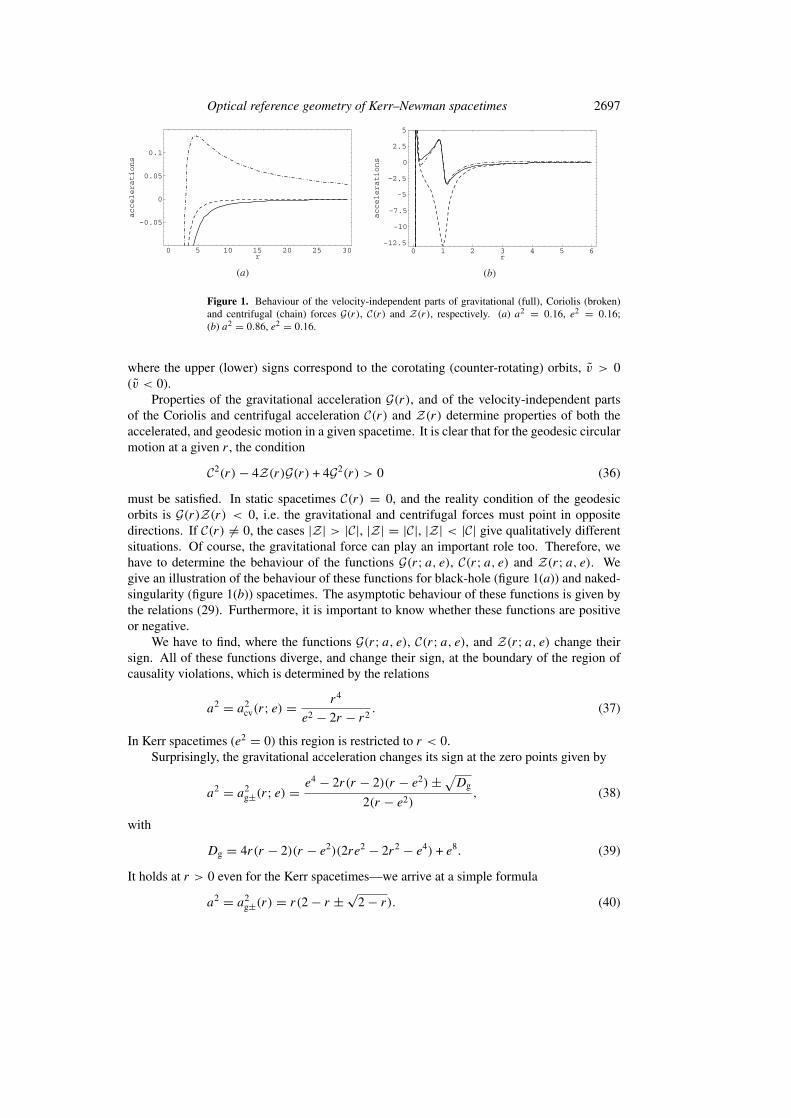
Figure 1. Behaviour of the velocity-independent parts of gravitational (full), Coriolis (broken)and centrifugal (chain) forces G(r), C(r) and Z(r), respectively. (a) a2 = 0.16, e2 = 0.16;(b) a2 = 0.86, e2 = 0.16.
where the upper (lower) signs correspond to the corotating (counter-rotating) orbits, v > 0(v < 0).
Properties of the gravitational acceleration G(r), and of the velocity-independent partsof the Coriolis and centrifugal acceleration C(r) and Z(r) determine properties of both theaccelerated, and geodesic motion in a given spacetime. It is clear that for the geodesic circularmotion at a given r , the condition
C2(r)− 4Z(r)G(r) + 4G2(r) > 0 (36)
must be satisfied. In static spacetimes C(r) = 0, and the reality condition of the geodesicorbits is G(r)Z(r) < 0, i.e. the gravitational and centrifugal forces must point in oppositedirections. If C(r) �= 0, the cases |Z| > |C|, |Z| = |C|, |Z| < |C| give qualitatively differentsituations. Of course, the gravitational force can play an important role too. Therefore, wehave to determine the behaviour of the functions G(r; a, e), C(r; a, e) and Z(r; a, e). Wegive an illustration of the behaviour of these functions for black-hole (figure 1(a)) and naked-singularity (figure 1(b)) spacetimes. The asymptotic behaviour of these functions is given bythe relations (29). Furthermore, it is important to know whether these functions are positiveor negative.
We have to find, where the functions G(r; a, e), C(r; a, e), and Z(r; a, e) change theirsign. All of these functions diverge, and change their sign, at the boundary of the region ofcausality violations, which is determined by the relations
a2 = a2cv(r; e) = r4
e2 − 2r − r2. (37)
In Kerr spacetimes (e2 = 0) this region is restricted to r < 0.Surprisingly, the gravitational acceleration changes its sign at the zero points given by
a2 = a2g±(r; e) = e4 − 2r(r − 2)(r − e2)± √
Dg
2(r − e2), (38)
with
Dg = 4r(r − 2)(r − e2)(2re2 − 2r2 − e4) + e8. (39)
It holds at r > 0 even for the Kerr spacetimes—we arrive at a simple formula
a2 = a2g±(r) = r(2 − r ± √
2 − r). (40)
2698 Z Stuchlık et al
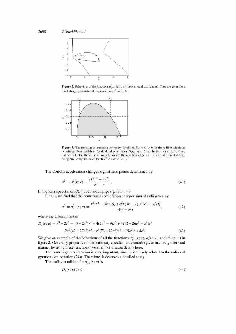
Figure 2. Behaviour of the functions a2g± (full), a2
c (broken) and a2z± (chain). They are given for a
fixed charge parameter of the spacetime, e2 = 0.16.
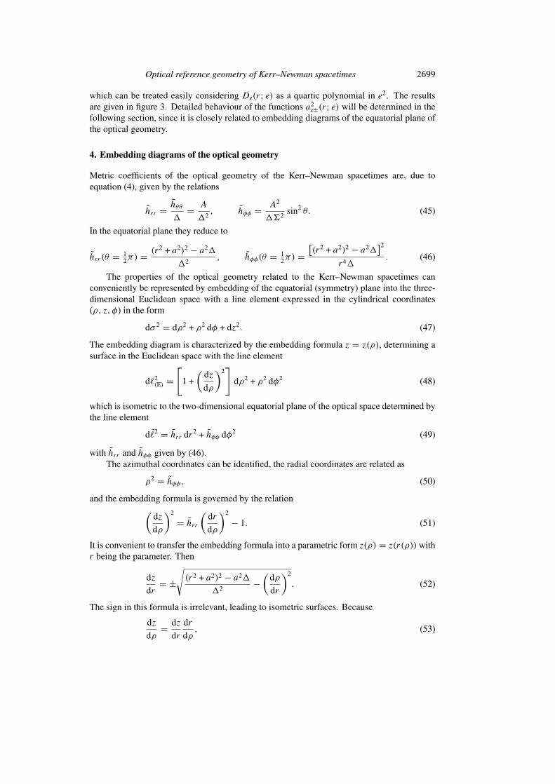
Figure 3. The function determining the reality condition Dz(r; e) � 0 for the radii at which thecentrifugal force vanishes. Inside the shaded region Dz(r; e) < 0 and the functions a2
z±(r; e) arenot defined. The three remaining solutions of the equation Dz(r; e) = 0 are not presented here,being physically irrelevant (with a2 < 0 or e2 < 0).
The Coriolis acceleration changes sign at zero points determined by
a2 = a2c (r; e) = r(3r2 − 2e2)
e2 − r. (41)
In the Kerr spacetimes, C(r) does not change sign at r > 0.Finally, we find that the centrifugal acceleration changes sign at radii given by
a2 = a2z±(r; e) = r2(r2 − 3r + 6) + e2r(3r − 7) + 2e4 ± √
Dz
4(r − e2), (42)
where the discriminant is
Dz(r; e) = r8 + 2r7 − (3 + 2e2)r6 + 4(2e2 − 9)r5 + 3(12 + 26e2 − e4)r4
−2e2(42 + 27e2)r3 + e4(73 + 12e2)r2 − 28e6r + 4e8. (43)
We give an example of the behaviour of all the functions a2g±(r; e), a2
c (r; e) and a2z±(r; e) in
figure 2. Generally, properties of the stationary circular motion can be given in a straightforwardmanner by using these functions; we shall not discuss details here.
The centrifugal acceleration is very important, since it is closely related to the radius ofgyration (see equation (24)). Therefore, it deserves a detailed study.
The reality condition for a2z±(r; e) is
Dz(r; e) � 0, (44)
Optical reference geometry of Kerr–Newman spacetimes 2699
which can be treated easily considering Dz(r; e) as a quartic polynomial in e2. The resultsare given in figure 3. Detailed behaviour of the functions a2
z±(r; e) will be determined in thefollowing section, since it is closely related to embedding diagrams of the equatorial plane ofthe optical geometry.
4. Embedding diagrams of the optical geometry
Metric coefficients of the optical geometry of the Kerr–Newman spacetimes are, due toequation (4), given by the relations
hrr = hθθ
!= A
!2, hφφ = A2
!�2sin2 θ. (45)
In the equatorial plane they reduce to
hrr (θ = 12π) = (r2 + a2)2 − a2!
!2, hφφ(θ = 1
2π) =[(r2 + a2)2 − a2!
]2
r4!. (46)
The properties of the optical geometry related to the Kerr–Newman spacetimes canconveniently be represented by embedding of the equatorial (symmetry) plane into the three-dimensional Euclidean space with a line element expressed in the cylindrical coordinates(ρ, z, φ) in the form
dσ 2 = dρ2 + ρ2 dφ + dz2. (47)
The embedding diagram is characterized by the embedding formula z = z(ρ), determining asurface in the Euclidean space with the line element
d+2(E) =
[1 +
(dz
dρ
)2]
dρ2 + ρ2 dφ2 (48)
which is isometric to the two-dimensional equatorial plane of the optical space determined bythe line element
d+2 = hrr dr2 + hφφ dφ2 (49)
with hrr and hφφ given by (46).The azimuthal coordinates can be identified, the radial coordinates are related as
ρ2 = hφφ, (50)
and the embedding formula is governed by the relation(dz
dρ
)2
= hrr
(dr
dρ
)2
− 1. (51)
It is convenient to transfer the embedding formula into a parametric form z(ρ) = z(r(ρ))withr being the parameter. Then
dz
dr= ±
√(r2 + a2)2 − a2!
!2−
(dρ
dr
)2
. (52)
The sign in this formula is irrelevant, leading to isometric surfaces. Because
dz
dρ= dz
dr
dr
dρ, (53)
2700 Z Stuchlık et al
the turning points of the embedding diagram, giving its throats and bellies, are determined bythe condition dρ/dr = 0, where
dρ
dr= {r4[r(r − 3) + 2e2] + a2[2e4 + e2r(3r − 7) + r2(r2 − 3r + 6)]
−2a4(r − e2)}[r3(r2 − 2r + a2 + e2)3/2]. (54)
By comparing equations (28) and (54) we can immediately see that turning points of theembedding diagrams are really located at the radii where the centrifugal force vanishes andchanges sign. Thus, we can conclude that just this property of embeddings of the opticalgeometry of the vacuum spherically symmetric spacetimes (see [1, 10, 13]) survives in theKerr–Newman spacetimes. However, photon circular orbits are displaced from the radii,corresponding to the turning points of the embedding diagrams. Therefore, it is interesting tofind the situations where the photon circular orbits lie within the regions of embeddability ofthe optical geometry.
4.1. Limits of embeddability
The embeddability condition (dz/dr)2 � 0 (see (52)) implies the relation
E(r; a, e) = 4r11 − 3(e2 + 3)r10 + 12(a2 + e2)r9
−2(17a2 + 5a2e2 + 2e4)r8 + 4(9a2 + 3a4 + 12a2e2)r7
−(33a4 + 66a2e2 + 11a4e2 + 17a2e4)r6
+4(9a4 + a6 + 13a4e2 + 10a2e4)r5
−(36a4 + 12a6 + 78a4e2 + 4a6e2 + 21a4e4 + 8a2e6)r4
+2(12a6 + 42a4e2 + 12a6e2 + 27a4e4)r3
−(4a8 + 52a6e2 + 73a4e4 + 12a6e4 + 12a4e6)r2
+4(2a8e2 + 9a6e4 + 7a4e6)r − 4(a8e4 + 2a6e6 + a4e8) � 0. (55)
The function E(r; a, e) can be considered as a polynomial quartic both in a2 and e2. Fore2 = 0, the function E(r; a) is still a polynomial quartic in a2 (see [15] for details). However,for a2 = 0, the function E(r; e) simplifies significantly, being only a polynomial quadratic ine2,
E(r; e) = r8[r2(4r − 9) + 3r(4 − r)e2 − 4e4]; (56)
its behaviour is discussed in [10]. For a2 = e2 = 0 we arrive at the well known Schwarzschildcondition r � 9
4 .The limits of embeddability are determined by the conditionE(r; a, e) = 0, which can be
solved as a quartic equation in a2. Let us denote the four solutions as a2ek(r; e), k ∈ {1, 2, 3, 4}.
Instead of giving long explicit expressions for the four solutions a2ek(r; e) we will treat them
numerically and classify qualitatively; different types of their behaviour will be described. Ofcourse, we naturally restrict our attention to physically relevant situations when a2 � 0 ande2 � 0.
Recall that if e2 = 0, the limits of embeddability are given by the solutions a2e3(r), a
2e4(r)
representing two branches, both reaching zero at r = 0 (see figure 4). The upper branch (a2e4)
diverges for r → ∞. The lower one (a2e3) has a local minimum at r = 1, where a2
e(min) = 1,and two local maxima, a2
e(max,2) = 1.135 40 at r = 0.689 47, and a2e(max,1) = 1.075 43 at
Optical reference geometry of Kerr–Newman spacetimes 2701
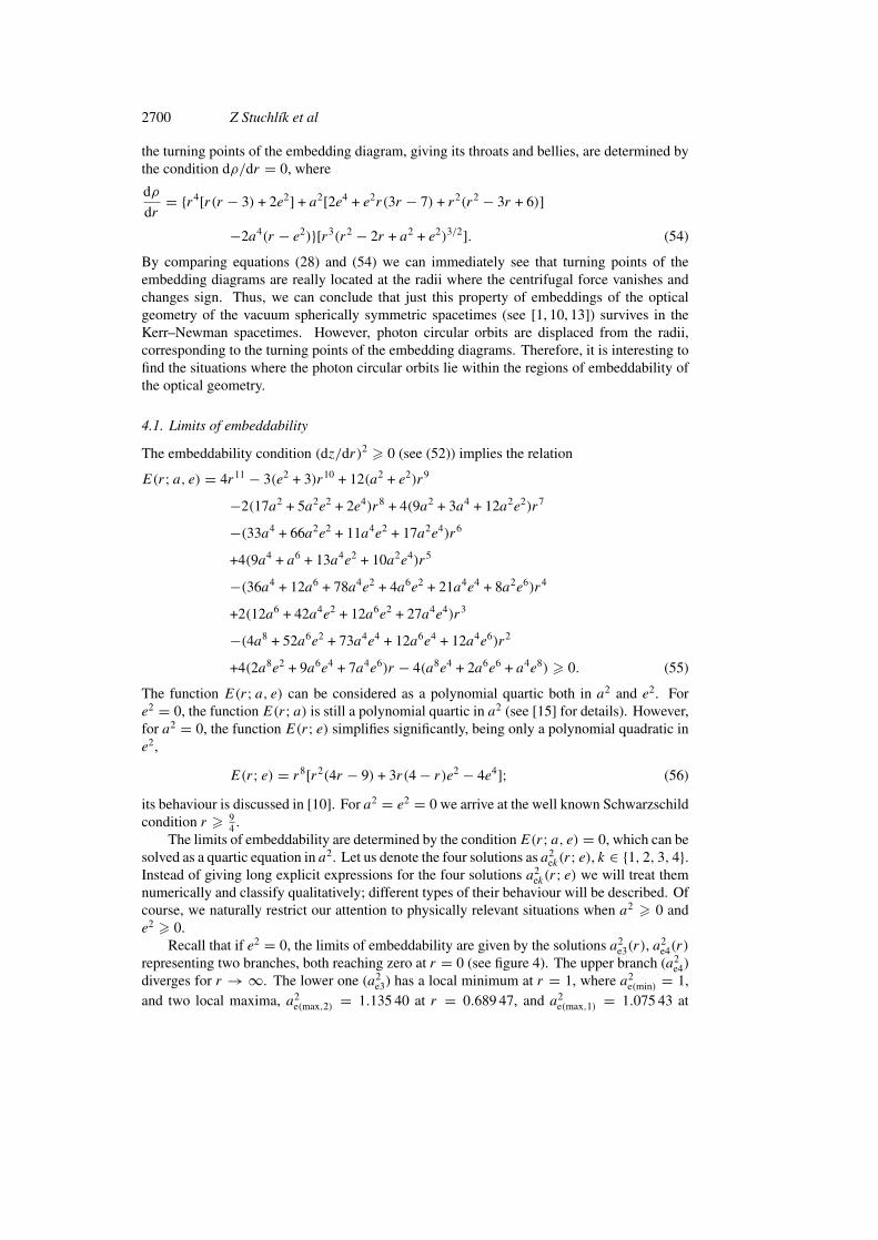
Figure 4. Square of the specific angular momentum of the Kerr backgrounds corresponding tothe event horizons (a2
h(r; e), the border between the dark-grey dynamic area, in which the opticalgeometry is not defined, and the light-grey non-embeddable area), photon circular orbits (a2
ph(r; e),broken curve), turning points of the embedding diagram (a2
z±(r; e), full curve), and embeddabilityregion border (a2
e (r; e), dotted curve enclosing the light-grey area not embeddable into Euclideanspace) are drawn as functions of the radius for fixed value e2 = 0.
Table 1. Subclassification of the Ea spacetimes according to the number of embeddable regions.
Subclass Interval of e2 Black holes Naked singularities
Ea1 〈0, 0.172 30) 1, 2, 3 4, 3, 2Ea2 〈0.172 30, 0.179 06) 1, 2 3, 4, 3, 2Ea3 〈0.179 06, 0.197 49) 1, 2 3, 2, 3, 2Ea4 〈0.197 49, 0.206 70) 1 2, 3, 2, 3, 2Ea5 〈0.206 70, 0.207 94) 1 2, 1, 2, 3, 2Ea6 〈0.207 94, 0.289 61) 1 2, 1, 2, 1, 2Ea7 〈0.289 61, 0.689 50) 1 2, 1, 2
r = 1.331 72; its second zero point is located at r = 2.25, corresponding to the Schwarzschildcase [15].
If e2 > 0, the limits of embeddability still consist of two branches. We can consider threequalitatively different situations.
4.1.1. Class Ea: e2 ∈ (0, 0.689 50). The two branches are given by the solutions a2e3(r; e)
and a2e4(r; e), again. Both the branches diverge at r = e2. The upper branch (a2
e4) also divergesfor r → ∞, having a local minimum a2
e4(min) near r = e2. The lower branch (a2e3) always
has a local minimum at r = 1, where a2e(min) = 1 − e2, corresponding to extreme black-hole
states, and a local maximum a2e(max,1) > 1 − e2 at r > 1. Its zero point, corresponding to the
Reissner–Nordstrom case, is determined by E(r; e) = 0 (cf equation (56)). It can also havea local minimum a2
e3(min) and a local maximum a2e3(max,2) at r < 1. Positions of a2
e4(min) anda2
e3(min) relative to the value a2 = 1 − e2, and the relation between a2e4(min) and a2
e3(max,2), ora2
e3(max,1), determine different members of embeddable regions of the Kerr–Newman black-holeand naked-singularity spacetimes. In table 1 we give the subclassification of the spacetimeslisted by the number of embeddable regions according to the values of the parameter e2; forfixed e2 from a given interval, the numbers of the embeddable regions are given with theparameter a2 growing.
2702 Z Stuchlık et al
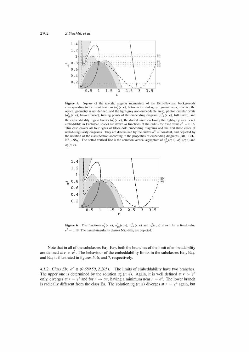
Figure 5. Square of the specific angular momentum of the Kerr–Newman backgroundscorresponding to the event horizons (a2
h(r; e), between the dark-grey dynamic area, in which theoptical geometry is not defined, and the light-grey non-embeddable area), photon circular orbits(a2
ph(r; e), broken curve), turning points of the embedding diagram (a2z±(r; e), full curve), and
the embeddability region border (a2e (r; e), the dotted curve enclosing the light-grey area is not
embeddable in Euclidean space) are drawn as functions of the radius for fixed value e2 = 0.16.This case covers all four types of black-hole embedding diagrams and the first three cases ofnaked-singularity diagrams. They are determined by the curves a2 = constant, and depicted bythe notation of the classification according to the properties of embedding diagrams (BH1–BH4,NS1–NS3). The dotted vertical line is the common vertical asymptote of a2
ph(r; e), a2c±(r; e) and
a2e (r; e).
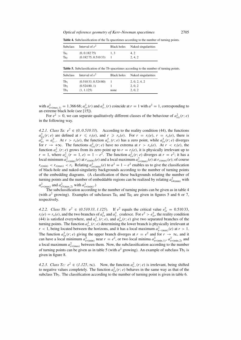
Figure 6. The functions a2h(r; e), a2
ph(r; e), a2c±(r; e) and a2
e (r; e) drawn for a fixed value
e2 = 0.19. The naked-singularity classes NS4–NS6 are depicted.
Note that in all of the subclasses Ea1–Ea7, both the branches of the limit of embeddabilityare defined at r > e2. The behaviour of the embeddability limits in the subclasses Ea1, Ea3,and Ea6 is illustrated in figures 5, 6, and 7, respectively.
4.1.2. Class Eb: e2 ∈ (0.689 50, 2.205). The limits of embeddability have two branches.The upper one is determined by the solution a2
e4(r; e). Again, it is well defined at r > e2
only, diverges at r = e2 and for r → ∞, having a minimum near r = e2. The lower branchis radically different from the class Ea. The solution a2
e3(r; e) diverges at r = e2 again, but

Optical reference geometry of Kerr–Newman spacetimes 2703
Figure 7. The functions a2h(r; e), a2
ph(r; e), a2c±(r; e) and a2
e (r; e) drawn for a fixed value
e2 = 0.25. The naked-singularity classes NS7–NS10 are depicted.
Table 2. Subclassification of the Eb spacetimes according to the number of embeddable regions.
Subclass Interval of e2 Black holes Naked singularities
Eb1 〈0.689 50, 1) 1 2, 1, 2Eb2 〈1, 2.205) None 1, 2
Table 3. Subclassification of the Ec spacetimes according to the number of embeddable regions.
Subclass Interval of e2 Black holes Naked singularities
Ec1 〈2.205,∞) None 1, 2
it has a discontinuity, which is ‘filled up’ by various combinations of the solutions a2e1(r; e),
a2e2(r; e) and a2
e4(r; e). The combinations depend on the parameter e2. However, it is not worthdiscussing them explicitly because they have common basic properties. They have no localextrema, but two lobes—an external (upper) one, and an internal (lower) one. The internallobe can enter the region of r < e2 for e2 high enough; for e2 > 1, the internal lobe is shiftedto the physically irrelevant region, where a2 < 0. If e2 < 1, the solution a2
e3(r; e) has a localminimum at r = 1, with a2 = 1 − e2 corresponding to an extreme black hole, and a localmaximum a2
e(max,1) > 1 − e2 at r > 1; for e2 = 1 these local extrema coalesce at r = 1,a2
e3 = 0. Therefore, the subclassification according to the number of embeddable regions canbe given as shown in table 2 (with a2 growing). An example of subclass Eb1 can be seen infigure 8.
4.1.3. Class Ec: e2 ∈ (2.205,∞). The limits of embeddability a2e (r; e) have two branches,
again. However, now both the branches are determined by the solution a2e4(r; e). The first
branch is defined at r > e2, diverges at r = e2 and for r → ∞, having a local minimum nearr = e2. The second branch is relevant from some r < e2, where a2
e4 = 0, and it diverges atr = e2, having no local extreme. The subclassification according to the number of embeddableregions is simply given just by one case (with a2 growing); see table 3.
Note that in situations which are necessary in order to construct typical embeddingdiagrams, the curves a2
e (r; e) are given explicitly (see figures 5–8). The behaviour of the

2704 Z Stuchlık et al
Figure 8. The functions a2h(r; e), a2
ph(r; e), a2c±(r; e) and a2
e (r; e) drawn for a fixed value
e2 = 0.92. In contrast to the preceding cases, there exist lobes of a2e (r; e), and a2
z±(r; e) is definedfor all r � e2. However, there exists an interval of the parameter a2 corresponding to naked-singularity spacetimes, at which no turning points appear on the embedding diagrams—these arethe NS11 spacetimes.
embeddability limits of the class Ec is not illustrated because they give no qualitatively differentkind of embedding diagrams.
4.2. Turning points of the embedding diagrams
The embeddable regions are characterized by the number of radii where the embeddingdiagrams have turning points, or, equivalently, where the centrifugal force determined by(28) vanishes. Therefore, the turning points of the diagrams are governed by the functionsa2
z±(r; e) determined by (42) and (43). We shall discuss the behaviour of these functions andintroduce a corresponding classification of the Kerr–Newman backgrounds (relative to theirparameter e2) according to the number of turning points of the embedding diagrams of theiroptical geometry.
It follows from the reality condition (44) (see also figure 3) that for e2 < e2cr = 0.510 33
the functions a2c±(r; e) are not defined between the radii ri(e), ro(e), i.e. inside the shaded
region in figure 3. If e2 = 0 (see figure 4), there is a2c±(r = 0) = 0 and a2
c−(r = 3) = 0.The part of a2
c−(r, 0) starting at r = 0 is located in the region between the horizons, and,therefore, is physically irrelevant; a local maximum of a2
z+(r) is located at r(max,1) = 0.811 59
Optical reference geometry of Kerr–Newman spacetimes 2705
Table 4. Subclassification of the Ta spacetimes according to the number of turning points.
Subclass Interval of e2 Black holes Naked singularities
Ta1 〈0, 0.182 75) 1, 3 4, 2Ta2 〈0.182 75, 0.510 33) 1 2, 4, 2
Table 5. Subclassification of the Tb spacetimes according to the number of turning points.
Subclass Interval of e2 Black holes Naked singularities
Tb1 〈0.510 33, 0.524 80) 1 2, 0, 2, 4, 2Tb2 〈0.524 80, 1) 1 2, 0, 2Tb3 〈1, 1.125) none 2, 0, 2
with a2z+(max,1) = 1.366 68; a2
c+(r) and a2z−(r) coincide at r = 1 with a2 = 1, corresponding to
an extreme black hole (see [15]).For e2 > 0, we can separate qualitatively different classes of the behaviour of a2
z±(r; e)in the following way.
4.2.1. Class Ta: e2 ∈ (0, 0.510 33). According to the reality condition (44), the functionsa2
z±(r; e) are defined at r � ri(e), and r � ro(e). For r = ri(e), r = ro(e), there isa2
z+ = a2c−. At r > ro(e), the function a2
z−(r; e) has a zero point, while a2z+(r; e) diverges
for r → +∞. The functions a2c±(r; e) have no extrema at r > ro(e). At r < ri(e), the
function a2z−(r; e) grows from its zero point up to r = ri(e), it is physically irrelevant up to
r = 1, where a2z−(r = 1, e) = 1 − e2. The function a2
c+(r; e) diverges at r = e2; it has alocal minimum a2
c+(min)(e) at rz(min)(e) and a local maximum a2c+(max)(e) at rc(max)(e); of course
rz(min) < rz(max) < ri. Relating a2z+(min)(e) to a2 = 1 − e2 enables us to give the classification
of black-hole and naked-singularity backgrounds according to the number of turning pointsof the embedding diagrams. (A classification of these backgrounds relating the number ofturning points and the number of embeddable regions can be realized by relating a2
e4(min) witha2
c+(max) and a2e3(max,2) with a2
z+(min).)The subclassification according to the number of turning points can be given as in table 4
(with a2 growing). Examples of subclasses Ta1 and Ta2 are given in figures 5 and 6 or 7,respectively.
4.2.2. Class Tb: e2 ∈ (0.510 33, 1.125). If e2 equals the critical value e2cr = 0.510 33,
ri(e) = ro(e), and the two branches of a2c+ and a2
z− coalesce. For e2 > e2cr, the reality condition
(44) is satisfied everywhere, and a2c−(r; e), and a2
z+(r; e) give two separated branches of theturning points. The function a2
z−(r; e) determining the lower branch is physically irrelevant atr < 1, being located between the horizons, and it has a local maximum a2
z−(max)(e) at r > 1.The function a2
z+(r; e) giving the upper branch diverges at r = e2 and for r → ∞, and itcan have a local minimum a2
z+(min) near r = e2, or two local minima a2z+(min,1), a
2z+(min,2) and
a local maximum a2c+(max) between them. Now, the subclassification according to the number
of turning points can be given as in table 5 (with a2 growing). An example of subclass Tb2 isgiven in figure 8.
4.2.3. Class Tc: e2 ∈ (1.125,∞). Now, the function a2c−(r; e) is irrelevant, being shifted
to negative values completely. The function a2c+(r; e) behaves in the same way as that of the
subclass Tb3. The classification according to the number of turning point is given in table 6.
2706 Z Stuchlık et al
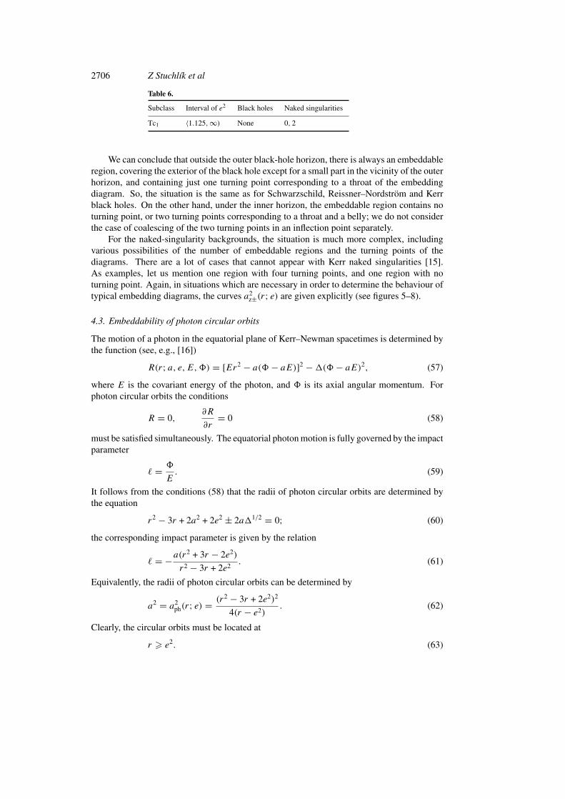
Table 6.
Subclass Interval of e2 Black holes Naked singularities
Tc1 〈1.125,∞) None 0, 2
We can conclude that outside the outer black-hole horizon, there is always an embeddableregion, covering the exterior of the black hole except for a small part in the vicinity of the outerhorizon, and containing just one turning point corresponding to a throat of the embeddingdiagram. So, the situation is the same as for Schwarzschild, Reissner–Nordstrom and Kerrblack holes. On the other hand, under the inner horizon, the embeddable region contains noturning point, or two turning points corresponding to a throat and a belly; we do not considerthe case of coalescing of the two turning points in an inflection point separately.
For the naked-singularity backgrounds, the situation is much more complex, includingvarious possibilities of the number of embeddable regions and the turning points of thediagrams. There are a lot of cases that cannot appear with Kerr naked singularities [15].As examples, let us mention one region with four turning points, and one region with noturning point. Again, in situations which are necessary in order to determine the behaviour oftypical embedding diagrams, the curves a2
z±(r; e) are given explicitly (see figures 5–8).
4.3. Embeddability of photon circular orbits
The motion of a photon in the equatorial plane of Kerr–Newman spacetimes is determined bythe function (see, e.g., [16])
R(r; a, e, E,�) = [Er2 − a(�− aE)]2 −!(�− aE)2, (57)
where E is the covariant energy of the photon, and � is its axial angular momentum. Forphoton circular orbits the conditions
R = 0,∂R
∂r= 0 (58)
must be satisfied simultaneously. The equatorial photon motion is fully governed by the impactparameter
+ = �
E. (59)
It follows from the conditions (58) that the radii of photon circular orbits are determined bythe equation
r2 − 3r + 2a2 + 2e2 ± 2a!1/2 = 0; (60)
the corresponding impact parameter is given by the relation
+ = −a(r2 + 3r − 2e2)
r2 − 3r + 2e2. (61)
Equivalently, the radii of photon circular orbits can be determined by
a2 = a2ph(r; e) = (r2 − 3r + 2e2)2
4(r − e2). (62)
Clearly, the circular orbits must be located at
r � e2. (63)
Optical reference geometry of Kerr–Newman spacetimes 2707
The zero points of a2ph(r; e) are located at radii
r1(e) = 12 [3 − (9 − 8e2)1/2], r2(e) = 1
2 [3 + (9 − 8e2)1/2], (64)
giving photon circular orbits of Reissner–Nordstrom spacetimes. The extrema of a2ph(r; e) are
located at the zero points r1(e), r2(e) (if e2 < 98 ), at r = 1 (if e2 < 1) and at
r = 43e
2, (65)
where a minimum exists for e2 < 34 , a maximum for 3
4 < e2 < 9
8 , and a minimum for e2 � 98 .
At r = 43e
2, the value of a2ph(r; e) is given by the function
a2ex(e) = 1
27e2(8e2 − 9)2. (66)
The function a2ex(e) determines the boundary between Kerr–Newman spacetimes
containing different numbers of photon circular orbits. If e2 < 34 , there can be two or four
circular orbits in the black-hole spacetimes and two orbits in naked-singularity spacetimes.If 3
4 < e2 < 1, there are two circular orbits in black hole and two or four orbits in naked-singularity spacetimes. For the naked-singularity spacetimes with 1 < e2 < 9
8 , there are twoor four orbits; if e2 > 9
8 , there are zero or two orbits.In the case of extreme black holes (a2 + e2 = 1), the radii of photon circular orbits and
corresponding values of the impact parameter are
r = 1, + = a + 1/a,
r = 2 − 2a, + = 4 − 3a,
r = 2 + 2a, + = −(4 + 3a).
(67)
The counter-rotating orbit at r = 2 + 2a is always located above the horizon. The corotatingorbit at r = 2 − 2a is located above the horizon if e2 > 3
4 , and under the horizon if e2 < 34 .
There are two orbits at r = 1 if e2 < 34 , but no circular orbit at r = 1, if e2 > 3
4 (see [16] fordetails).
Now, we shall discuss in which cases the photon circular orbits enter the regions ofembeddability. Radii of the photon circular orbits are determined by the function a2
ph(r; e)given by equation (62). The embeddability of these orbits must be determined by a numericalprocedure. Note that, generally, the function a2
z−(r; e) has common points with a2ph(r; e) at its
zero points (if e2 < 98 ), and at r = 1 (if e2 < 1).
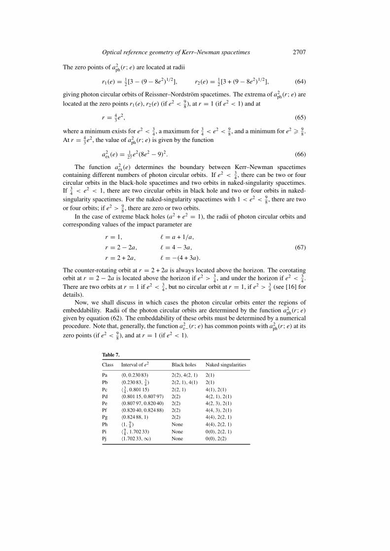
Table 7.
Class Interval of e2 Black holes Naked singularities
Pa 〈0, 0.230 83) 2(2), 4(2, 1) 2(1)Pb 〈0.230 83, 3
4 ) 2(2, 1), 4(1) 2(1)Pc 〈 3
4 , 0.801 15) 2(2, 1) 4(1), 2(1)Pd 〈0.801 15, 0.807 97) 2(2) 4(2, 1), 2(1)Pe 〈0.807 97, 0.820 40) 2(2) 4(2, 3), 2(1)Pf 〈0.820 40, 0.824 88) 2(2) 4(4, 3), 2(1)Pg 〈0.824 88, 1) 2(2) 4(4), 2(2, 1)Ph 〈1, 9
8 ) None 4(4), 2(2, 1)
Pi 〈 98 , 1.702 33) None 0(0), 2(2, 1)
Pj 〈1.702 33,∞) None 0(0), 2(2)
2708 Z Stuchlık et al
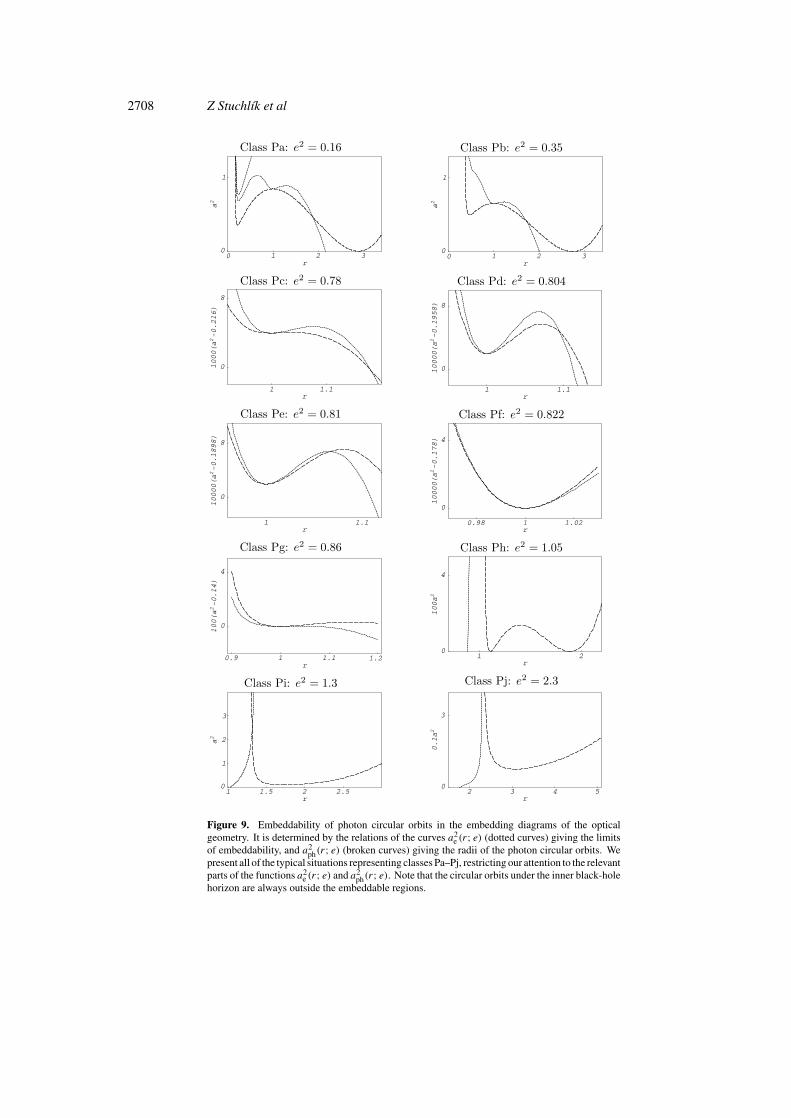
Figure 9. Embeddability of photon circular orbits in the embedding diagrams of the opticalgeometry. It is determined by the relations of the curves a2
e (r; e) (dotted curves) giving the limitsof embeddability, and a2
ph(r; e) (broken curves) giving the radii of the photon circular orbits. Wepresent all of the typical situations representing classes Pa–Pj, restricting our attention to the relevantparts of the functions a2
e (r; e) and a2ph(r; e). Note that the circular orbits under the inner black-hole
horizon are always outside the embeddable regions.
Optical reference geometry of Kerr–Newman spacetimes 2709
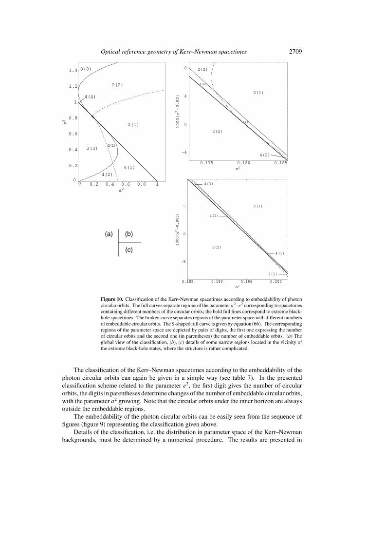
Figure 10. Classification of the Kerr–Newman spacetimes according to embeddability of photoncircular orbits. The full curves separate regions of the parameter a2–e2 corresponding to spacetimescontaining different numbers of the circular orbits; the bold full lines correspond to extreme black-hole spacetimes. The broken curve separates regions of the parameter space with different numbersof embeddable circular orbits. The S-shaped full curve is given by equation (66). The correspondingregions of the parameter space are depicted by pairs of digits, the first one expressing the numberof circular orbits and the second one (in parentheses) the number of embeddable orbits. (a) Theglobal view of the classification, (b), (c) details of some narrow regions located in the vicinity ofthe extreme black-hole states, where the structure is rather complicated.
The classification of the Kerr–Newman spacetimes according to the embeddability of thephoton circular orbits can again be given in a simple way (see table 7). In the presentedclassification scheme related to the parameter e2, the first digit gives the number of circularorbits, the digits in parentheses determine changes of the number of embeddable circular orbits,with the parameter a2 growing. Note that the circular orbits under the inner horizon are alwaysoutside the embeddable regions.
The embeddability of the photon circular orbits can be easily seen from the sequence offigures (figure 9) representing the classification given above.
Details of the classification, i.e. the distribution in parameter space of the Kerr–Newmanbackgrounds, must be determined by a numerical procedure. The results are presented in

2710 Z Stuchlık et al
Figure 11. Embedding diagram of the Kerr–Newman black holes of the type BH1, constructedfor a2 = 0.16, e2 = 0.16. The rings in the 3D diagram represent photon circular orbits. Bothcorotating (grey circle in the 2D diagram) and counter-rotating (full circle in the 2D diagram) aredisplaced from the throat of the diagram, where the centrifugal force vanishes. This is a generalproperty of the rotating backgrounds.
figure 10. The regions of the parameter plane a2–e2 are denoted by two digits. The first onegives the number of photon circular orbits in the corresponding background, the second one(in parentheses) gives the number of embeddable orbits.
4.4. Construction of the embedding diagrams
The relevant properties of the embedding diagrams are determined by the functions a2e (r; e)
and a2z (r; e) governing embeddable parts of the optical reference geometry and turning points
of the diagrams. We shall present a classification of the Kerr–Newman spacetimes accordingto the number of embeddable regions and the number of turning points. All cases of theclassification will be represented by a typical embedding diagram. Inspecting all of the typesof behaviour of functions a2
c±(r; e) (given by classes Ta–Tc and their subclasses), we findthat there are four cases of the behaviour of the embeddings for the black-hole spacetimes,and 11 cases for the naked-singularity spacetimes. A complete list of typical embeddingswill be given by using the behaviour of the characteristic functions a2
e (r; e) and a2z (r; e) for
some typical values of the parameter e2 (see figures 5–8), where the functions a2h(r; e) and
a2ph(r; e) are included for completeness. In order to obtain all 15 types of embedding diagrams,
it is necessary to consider at least four values of the parameter e2 belonging subsequently tothe subclasses Ea1 (e2 = 0.16), Ea3 (e2 = 0.19), Ea6 (e2 = 0.25), Eb1 (e2 = 0.92) of theclassification according to the number of embeddable regions, discussed above. The behaviourof a2
c (r; e) for these four values of e2 enables us to present a complete list of typical embeddingdiagrams. The classes will be denoted successively by a growing parameter a2 for each fixede2.
In the regions of the optical geometry where the embeddability condition E(r; a, e) � 0is satisfied, the embedding diagram can be constructed for a fixed parameter a by integratingthe parametrically expressed embedding formula z(r) (cf equation (52)), and transferring itinto the final form z(ρ) by an appropriate numerical procedure using (50). In all the typical
Optical reference geometry of Kerr–Newman spacetimes 2711
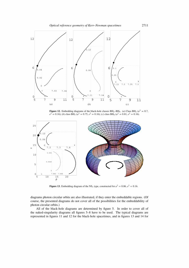
Figure 12. Embedding diagrams of the black-hole classes BH2–BH4. (a) Class BH2 (a2 = 0.7,e2 = 0.16); (b) class BH3 (a2 = 0.75, e2 = 0.16); (c) class BH4 (a2 = 0.81, e2 = 0.16).
Figure 13. Embedding diagram of the NS1 type, constructed for a2 = 0.86, e2 = 0.16.
diagrams photon circular orbits are also illustrated, if they enter the embeddable regions. (Ofcourse, the presented diagrams do not cover all of the possibilities for the embeddability ofphoton circular orbits.)
All of the black-hole diagrams are determined by figure 5. In order to cover all ofthe naked-singularity diagrams all figures 5–8 have to be used. The typical diagrams arerepresented in figures 11 and 12 for the black-hole spacetimes, and in figures 13 and 14 for
2712 Z Stuchlık et al
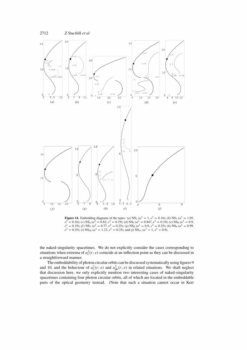
Figure 14. Embedding diagrams of the types: (a) NS2 (a2 = 1, e2 = 0.16); (b) NS3 (a2 = 1.05,e2 = 0.16); (c) NS4 (a2 = 0.82, e2 = 0.19); (d) NS5 (a2 = 0.847, e2 = 0.19); (e) NS6 (a2 = 0.9,e2 = 0.19); (f ) NS7 (a2 = 0.77, e2 = 0.25); (g) NS8 (a2 = 0.9, e2 = 0.25); (h) NS9 (a2 = 0.99,e2 = 0.25); (i) NS10 (a2 = 1.23, e2 = 0.25); and (j) NS11 (a2 = 1, e2 = 0.9).
the naked-singularity spacetimes. We do not explicitly consider the cases corresponding tosituations when extrema of a2
e (r; e) coincide at an inflection point as they can be discussed ina straightforward manner.
The embeddability of photon circular orbits can be discussed systematically using figures 9and 10, and the behaviour of a2
e (r; e) and a2ph(r; e) in related situations. We shall neglect
that discussion here, we only explicitly mention two interesting cases of naked-singularityspacetimes containing four photon circular orbits, all of which are located in the embeddableparts of the optical geometry instead. (Note that such a situation cannot occur in Kerr
Optical reference geometry of Kerr–Newman spacetimes 2713
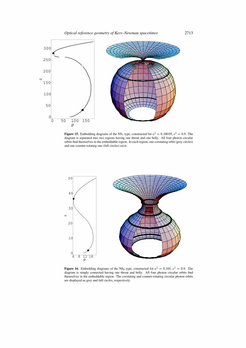
Figure 15. Embedding diagrams of the NS7 type, constructed for a2 = 0.100 05, e2 = 0.9. Thediagram is separated into two regions having one throat and one belly. All four photon circularorbits find themselves in the embeddable region. In each region, one corotating orbit (grey circles)and one counter-rotating one (full circles) exist.
Figure 16. Embedding diagrams of the NS8 type, constructed for a2 = 0.105, e2 = 0.9. Thediagram is simply connected having one throat and belly. All four photon circular orbits findthemselves in the embeddable region. The corotating and counter-rotating circular photon orbitsare displayed as grey and full circles, respectively.
2714 Z Stuchlık et al
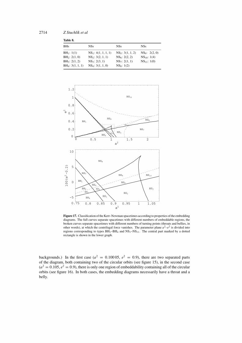
Table 8.
BHs NSs NSs NSs
BH1: 1(1) NS1: 4(1, 1, 1, 1) NS5: 3(1, 1, 2) NS9: 2(2, 0)BH2: 2(1, 0) NS2: 3(2, 1, 1) NS6: 2(2, 2) NS10: 1(4)BH3: 2(1, 2) NS3: 2(3, 1) NS7: 2(1, 1) NS11: 1(0)BH4: 3(1, 1, 1) NS4: 3(1, 1, 0) NS8: 1(2)
Figure 17. Classification of the Kerr–Newman spacetimes according to properties of the embeddingdiagrams. The full curves separate spacetimes with different numbers of embeddable regions, thebroken curves separate spacetimes with different numbers of turning points (throats and bellies, inother words), at which the centrifugal force vanishes. The parameter plane a2–e2 is divided intoregions corresponding to types BH1–BH4 and NS1–NS11. The central part marked by a dottedrectangle is shown in the lower graph.
backgrounds.) In the first case (a2 = 0.100 05, e2 = 0.9), there are two separated partsof the diagram, both containing two of the circular orbits (see figure 15), in the second case(a2 = 0.105, e2 = 0.9), there is only one region of embeddability containing all of the circularorbits (see figure 16). In both cases, the embedding diagrams necessarily have a throat and abelly.
Optical reference geometry of Kerr–Newman spacetimes 2715
4.5. The classification
The following classification will be made according to the properties of the embeddingdiagrams. The Kerr–Newman spacetimes are characterized by the number of embeddableregions of the optical geometry, and by the number of turning points at these regions, givensuccessively for the regions with descending radial coordinate of the geometry (which arepresented in parentheses). Therefore, the classification can be given in table 8.
The parameter space of the Kerr–Newman spacetimes can be separated into regionscorresponding to the classes BH1–BH4, and NS1–NS11 by a numerical code expressing theextreme points of the functions a2
e (r; e) and a2c (r; e) as functions of e2. Results of the numerical
code are presented in figure 17, which represents the classification completely.
5. Concluding remarks
In the rotating black-hole and naked-singularity backgrounds, the embedding diagrams ofthe optical reference geometry reflect immediately just one important property of the inertialforces related to a test-particle circular motion. Namely, the turning points of the embeddingdiagrams occur just at radii where the centrifugal force vanishes and reverses sign, independentof the velocity of the motion. However, in contrast to the spherically symmetric black-hole and naked-singularity backgrounds, in the rotating backgrounds the radii of the photoncircular orbits do not coincide with the radii of vanishing centrifugal force, and, moreover,in a variety of Kerr–Newman backgrounds, some of these orbits are even not located in theregions of the optical geometry that are embeddable into the three-dimensional Euclideanspace.
The properties of the embedding diagrams have been discussed, and a classificationscheme of the Kerr–Newman backgrounds reflecting the number of embeddable regions, andthe number of turning points of these regions, was presented. The ring singularity in all ofthe rotating backgrounds, and the horizons of the black-hole backgrounds, are always locatedoutside the embeddable regions. Further, embeddability of regions containing the photoncircular orbit has been established.
The presence of a non-zero charge parameter e in the Kerr–Newman backgrounds enrichessignificantly the variety of the embedding diagrams in comparison with the case of pure Kerrbackgrounds [15].
For the black-hole backgrounds, there is just one embeddable region outside the outerhorizon, containing just one throat. However, under the inner horizon, there can be two,one or no embeddable regions. They can have a throat and a belly. Above the outerhorizon, the outermost, counter-rotating photon circular orbit is always embeddable, whilethe inner, corotating one is embeddable in backgrounds with sufficiently small specificangular momentum, but non-embeddable in the other ones. On the other hand, the photoncircular orbits existing under the inner horizon are always located in the non-embeddableregions.
For the naked-singularity backgrounds, the variety of possible embedding diagrams ismuch more complex and can be read directly from figures 13 and 14. Let us point out themost important phenomena. There can exist diagrams consisting of four separated regions,or, oppositely, simply connected diagrams, having two throats and two bellies. On theother hand, there are also diagrams having no turning point. Moreover, in some naked-singularity backgrounds containing four photon circular orbits, all of the orbits are located inthe embeddable regions—such a situation is impossible in the black-hole backgrounds.
2716 Z Stuchlık et al
The embedding diagrams of the optical geometry give an important tool for thevisualization and clarification of the dynamical behaviour of test particles moving alongequatorial circular orbits, by imagining that the motion is constrained on the surface z(ρ)[10]. The shape of the surface z(ρ) is directly related to the centrifugal acceleration.Within the rising portions of the embedding diagram, the centrifugal acceleration pointstowards increasing values of r , and the dynamics of test particles has essentially a Newtoniancharacter. However, in the descending portions of the embedding diagrams, the centrifugalacceleration has a radically non-Newtonian character, as it points towards decreasing valuesof r . Such a kind of behaviour appears where the diagrams have a throat or a belly. At theturning points of the diagram, the centrifugal acceleration vanishes and changes its sign, i.e.dr/dρ = dz/dρ = 0.
We can understand this connection of the centrifugal force and the embedding of the opticalspace in terms of the radius of gyration representing rotational properties of rigid bodies. InNewtonian mechanics, it is defined as the radius R of the circular orbit on which a point-likeparticle having the same massM and angular velocity & as a rigid body would have the sameangular momentum J :
J = MR2&. (68)
Defining a specific angular momentum + = J/M , we obtain
R =√+
&. (69)
For a point-like particle moving on r = constant, there is R = r .In general relativity, the radius of a circle can be given in two standard ways; namely
as the circumferential radius and as the proper radial distance. A third way can be given bygeneralizing equation (69) for a point particle moving along r = constant; we use + = L/E,whereL is the angular momentum of the particle, andE is its energy. (In stationary spacetimes,the angular velocity has to be related to the family of locally non-rotating observers, cfequation (23).) In Newtonian theory, these three definitions of radius give identical results,however, in general relativity they are distinct. The radius of gyration R is convenient fordiscussing the dynamical effects of rotation; the direction of increase of R defines a localoutward direction for these effects. The surfaces R = constant, called von Zeipel cylinders,were proved to be a very useful concept in the theory of rotating fluids in stationary, axiallysymmetric spacetimes. In Newtonian theory, they are ordinary straight cylinders, but theirshape is deformed by general-relativistic effects, and their topology may be non-cylindrical.There is a critical family of self-crossing von Zeipel surfaces [20].
It is crucial that in the Kerr–Newman spacetimes
[hφφ(θ = π/2)]1/2 = ρ = R, (70)
i.e. the embedding diagrams of the equatorial plane of the optical geometry are expressed interms of the radius of gyration. Since in the equatorial plane the centrifugal acceleration hasthe radial component
Z(r) = R−1∂rR, (71)
the relation of the embedding diagrams, the radius of gyration, and the centrifugal force isclear. Note that the turning points of the embedding diagrams determine both the radii wherethe centrifugal force changes sign, and the radii of cusps where the critical von Zeipel surfacesare self-crossing. Therefore, the embedding diagrams also reflect the properties of a fluidrotating in Kerr–Newman spacetimes.

Optical reference geometry of Kerr–Newman spacetimes 2717
Note that the black-hole backgrounds have a unified character above the event horizon—there exists a throat of the embedding diagram indicating a change of sign of the centrifugalforce near the event horizon. On the other hand, the naked-singularity spacetimes give awide variety of behaviour of the embeddings and centrifugal forces, ranging from the simple‘Newtonian’ backgrounds with no change of sign of the centrifugal force, to very complicatedbackgrounds, where the sign changes four times.
We also established the embeddability of circular photon geodesics. There are many caseswhen these orbits are located in regions that are non-embeddable.
Note that because the photon circular geodesics are given by the condition Z(r)−C(r) = 0for corotating orbits, and Z(r) + C(r) = 0 for counter-rotating orbits, the corotating (counter-rotating) orbits are located on the descending (rising) portion of the embedding diagrams(assuming C(r) < 0), if they enter the embeddable regions (see figures 15 and 16).
Finally, it should be noted that in the case of the spherically symmetric spacetimes(Schwarzschild and Reissner–Nordstrom [10, 18, 21], and Schwarzschild–de Sitter [13, 22]),it can be shown that the limits of embeddability of the optical geometry coincide with theexistence limit of static configurations of uniform density. Unfortunately, we have not foundany evident connection between the embeddability limits of the diagrams and any otherphenomenon in the Kerr–Newman spacetimes. The search for such a phenomenon remains agreat challenge for future investigations.
Acknowledgments
This work has been partly supported by the GACR grant no 202/99/0261, the grant J10/98:192400004 and the committee for collaboration of Czech Republic with CERN. It hasbeen finished during visits at The Abdus Salam ICTP, Trieste, and CERN Theory Division,Geneva; the authors would like to thank both institutions for perfect hospitality. The authorswould also like to express their gratitude to Professor Marek Abramowicz for stimulatingdiscussions.
References
[1] Abramowicz M A, Carter B and Lasota J P 1988 Gen. Rel. Grav. 20 1173[2] Abramowicz M A, Nurowski P and Wex N 1993 Class. Quantum Grav. 10 L183[3] Semerak O 1995 Nuovo Cimento B 110 973[4] Jantzen R T, Carini P and Bini D 1992 Ann. Phys., NY 215 1[5] Abramowicz M A, Nurowski P and Wex N 1995 Class. Quantum Grav. 12 1467[6] Abramowicz M A and Prasanna A R 1990 Mon. Not. R. Astron. Soc. 245 720[7] Abramowicz M A, Miller J C and Stuchlık Z 1993 Phys. Rev. D 47 1440[8] Abramowicz M A 1990 Mon. Not. R. Astron. Soc. 245 733[9] Abramowicz M A 1992 Mon. Not. R. Astron. Soc. 256 710
[10] Kristiansson S, Sonego S and Abramowicz M A 1998 Gen. Rel. Grav. 30 275[11] Stuchlık Z and Hledık S 1999 Class. Quantum Grav. 16 1377[12] Bardeen J M 1973 Black Holes ed C De Witt and B S DeWitt (New York: Gordon and Breach)[13] Stuchlık Z and Hledık S 1999 Phys. Rev. D 60 044006[14] Iyer S and Prasanna A R 1993 Class. Quantum Grav. 10 L13[15] Stuchlık Z and Hledık S 1999 Acta Phys. Slovaca 49 795[16] Bicak J, Balek V and Stuchlık Z 1989 Bull. Astron. Inst. Czech. 40 133[17] Aguirregabiria J M, Chamorro A, Rajesh Nayak K, Suinaga J and Vishveshwara C V 1996 Class. Quantum
Grav. 13 2179[18] Misner C W, Thorne K S and Wheeler J A 1973 Gravitation (San Francisco, CA: Freeman)[19] Sonego S and Abramowicz M A 1998 J. Math. Phys. 39 3158[20] Kozlowski M, Jaroszynski M and Abramowicz M A 1978 Astron. Astrophys. 63 209
2718 Z Stuchlık et al
[21] de Felice F, Yu Y and Fang J 1995 Mon. Not. R. Astron. Soc. 277 L17[22] Stuchlık Z 1999 Spherically symmetric static configurations of uniform density in spacetimes with a non-zero
cosmological constant TPA 007 Preprint Silesian University at Opava (Acta Physica Slovaca to be published)(for see http://www.fpf.slu.cz/ hle10uf/rag/tpapps.html)